The effect of systematics on polarized spectral indices

Abstract

We study four particularly bright polarized compact objects (Tau A, Virgo A, 3C273 and Fornax A) in the 7-year WMAP sky maps, with the goal of understanding potential systematics involved in estimation of foreground spectral indices. We estimate the spectral index, the polarization angle, the polarization fraction and apparent size and shape of these objects when smoothed to a nominal resolution of $1^{\circ}$ FWHM. Second, we compute the spectral index as a function of polarization orientation, $\alpha$. Because these objects are approximately point sources with constant polarization angle, this function should be constant in the absence of systematics. However, for the K- and Ka-band WMAP data we find strong index variations for all four sources. For Tau A, we find a spectral index of $\beta=-2.59\pm 0.03$ for $\alpha=30^{\circ}$, and $\beta=-2.03\pm 0.01$ for $\alpha=50^{\circ}$. On the other hand, the spectral index between Ka- and Q-band is found to be stable. A simple elliptical Gaussian toy model with parameters matching those observed in Tau A reproduces the observed signal, and shows that the spectral index is in particular sensitive to the detector polarization angle. Based on these findings, we first conclude that estimation of spectral indices with the WMAP K-band polarization data at $1^{\circ}$ scales is not robust. Second, we note that these issues may be of concern for ground-based and sub-orbital experiments that use the WMAP polarization measurements of Tau A for calibration of gain and polarization angles.

1. Introduction

One of the central goals in contemporary observational cosmology is to detect the postulated background of primordial gravity waves predicted by inflation. The most direct observational signature of these gravity waves is a particular pattern in the polarization of the cosmic microwave background (CMB) known as B-modes. The amplitude of these gravity waves is typically parametrized in terms of the tensor-to-scalar ratio, $r$ (see, e.g. Liddle & Lyth, 2000, and references therein for a thorough review on inflation). During the last few years many experiments have been planned, built and fielded to measure $r$, and the first relevant B-mode constraints have been already published by BICEP ($r<0.7$, Chiang et al. 2010) and QUIET ($r<2.1$; QUIET 2011, 2012). Other ground-based and sub-orbital experiments are expected to vastly improve on these limits in the very near future.

In order to make an actual detection of the inflationary gravity waves, it is widely believed that a sensitivity of $r\lesssim 0.01$ will be required. In terms of map-domain sensitivity, this corresponds to a signal with an RMS of a few tens of nK. Thus, not only will exquisitely sensitive detectors be needed, but also detectors with extremely low systematics.

However, the single most problematic systematic for future B-mode experiments is likely not to come from the instrument itself, but rather from the sky: Non-cosmological Galactic and extra-galactic foregrounds, for instance synchrotron and thermal dust, radiates with a temperature of several $\mu\textrm{K}$ on large angular scales in the frequencies relevant for CMB measurements (e.g., Gold et al., 2011, and references therein). Therefore, in order not to be foreground dominated, these foregrounds must very likely be suppressed by perhaps an order of magnitude or more. The only way to achieve this is by making multifrequency observations of the same fields of the sky, and exploit the different frequency dependency of the various components to separate out the cosmological CMB signal from the non-cosmological foregrounds.

As of today, a very large fraction of the information we have about polarized foregrounds on large angular scales comes from the WMAP satellite experiment, and in particular the lowest frequency channel at 23 GHz (K-band). This map is routinely used both for studies of foregrounds themselves, and as ancillary data for other experiments. It is therefore critical to understand the systematic limitations inherent in these data. In this paper we measure the spectral indices of four particularly bright compact objects (Tau A, Virgo A, 3C273 and Fornax A), with the goal of understanding some of the issued involved in spectral index estimation for CMB data in general: By considering high signal-to-noise objects with known properties, we have a clear a-priori prediction, and deviations from these expectations would indicate either model problems or systematic errors.

2. Data and model

Sky maps and processing

In this paper we consider the 7-year WMAP sky maps (Jarosik et al., 2011), coadded over years and pixelized at a HEALPix resolution of $N_{\textrm{side}}=512$, corresponding to $7^{\prime}$ pixels. These data are available from LAMBDA, including all necessary ancillary data, such as beam profiles and noise model. Most of our analysis is performed with the K- and Ka-band data, although in one particular case we also consider the Q-band data. All analyses are carried out in antenna temperature units, and given that we will consider objects with steep synchrotron-like spectra we adopt effective frequencies of 22.45 GHz (K-band), 32.64 GHz (Ka-band) and 40.50 GHz (Q-band), respectively (Page et al., 2003).

Before one can estimate spectral indices across frequencies, it is necessary to bring all maps to a common angular resolution. We therefore smooth all maps to an effective resolution of $1^{\circ}$ FWHM by first deconvolving the instrument beam and then convolving with a Gaussian beam of the desired size. Note that the smoothing scale of $1^{\circ}$ is a particularly common value adopted in the literature, and the results presented here are therefore of wide interest.

Estimation of uncertainties for all scalar quantities is done by forward Monte Carlo simulations. That is, we add smoothed noise realizations to the actual WMAP data based on the provided noise model, evaluate each statistic for each simulation, and then compute the resulting standard deviation over the ensemble. Although there already is a noise component present in the WMAP data, this is identical for all simulations, and therefore do not contribute to the variance. We emphasize, though, that uncertainties estimated in this manner are only statistical in nature, and do not account for systematic errors.

Data selection

In this paper we consider the four particularly bright point sources listed in Table 1. These were selected by thresholding the K-band polarization map, $P=\sqrt{Q^{2}+U^{2}}$, at $100\mu\textrm{K}$, and discarding all regions that either show obviously extended features or have a strong background. This left us with Tau A as the only near-Galactic source, and three high-latitude sources (Virgo A, 3C273 and Fornax A). For further details on the polarization properties of these objects, see, e.g., Aumont et al. (2010); Weiland et al. (2011); Fomalont et al. (1989); Ekers et al. (1983); Rottmann et al. (1996).

Only pixels in a $1^{\circ}$ radius disc around each source were kept for analysis, although we also tried $2^{\circ}$ discs, obtaining consistent, but slightly more noisy, results. Note that a Gaussian beam of $1^{\circ}$ FWHM ($\sim 2.35\sigma$) has dropped off to 6% of its peak value at a distance of $1^{\circ}$, and most of the volume is therefore contained within this radius.

Data model

The low-frequency WMAP polarization observations are strongly dominated by synchrotron emission which has a sharply falling spectrum. We therefore approximate the total sky signal by a single power-law, resulting in the following data model,

$$\mathbf{d}_{\nu}=\mathbf{B}\mathbf{a}\left(\frac{\nu}{\nu_{0}}\right)^{\beta}+\mathbf{n}_{\nu}.$$ (1)

Here $\mathbf{d}_{\nu}$ is an $N_{\textrm{pix}}\times 3$ matrix listing the Stokes’ $I$, $Q$ and $U$ parameters for all relevant pixels at frequency $\nu$ columnwise, $\mathbf{B}$ is a $3N_{\textrm{pix}}\times 3N_{\textrm{pix}}$ matrix denoting convolution with the common instrumental beam, $\mathbf{a}$ denotes the true sky signal amplitude as measured at a reference frequency $\nu_{0}$, and $\mathbf{n}_{\nu}$ is (smoothed) instrumental noise. All values are defined in antenna temperature units. Coordinates are defined according to the HEALPix convention (Górski et al., 2005).

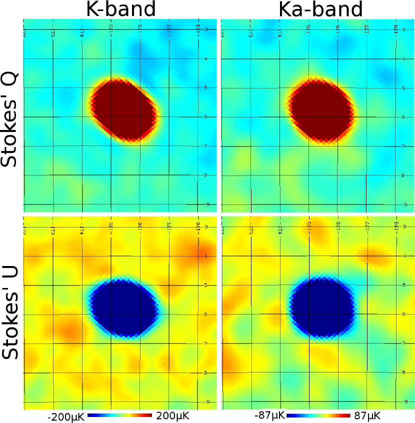
Figure 1.— Tau A as observed by the two lowest WMAP frequencies, and rotated into a coordinate system offset by $22.5^{\circ}$ from the intrinsic polarization direction of Tau A. Note both that the K-band images are significantly more asymmetric than the Ka-band images, and also that the two Stokes’ parameters within a single band are significantly different.

3. Methods

Given the data and model described in Section 2, we estimate the polarization angle and fraction, the spectral index and the apparent shape of each source. First, we note that each of the four objects considered here are well known in the literature, and have known polarization properties. Further, they are all known to be much smaller than $1^{\circ}$ in angular dimensions (see Table 1 for precise details), and their polarization angles are known to be quite stable as a function of frequency. (For example, the polarization angle of Tau A is known to vary by only a few degrees over more than 10 decades in frequency; e.g., Aumont et al. 2010.) We therefore assume that there is no real substructure within each source on the scales we consider.

Table 1Apparent object position, size and shape

	Longitude	Latitude	Size	FWHM (degrees)		Ellipticity		Orientation (degrees)
Object	(degrees)	(degrees)	(arcmin)	K	Ka	K	Ka	K	Ka
Tau A	$184.56$	$\,-5.78$	$7\times 5$	$0.985\pm 0.001$	$0.992\pm 0.001$	$0.142\pm 0.001$	$0.079\pm 0.001$	$54.0\pm 0.3$	$57.8\pm 1.5$
Virgo A	$283.78$	$\phantom{string}\phantom{.}74.49$	$8\times 6$	$0.91\pm 0.02$	$0.89\pm 0.05$	$0.17\pm 0.04$	$0.13\pm 0.06$	$76\pm 9$	$56\pm 33$
3C273	$289.95$	$\phantom{1}64.36$	$<1$	$1.05\pm 0.02$	$0.88\pm 0.05$	$0.14\pm 0.03$	$0.22\pm 0.07$	$117\pm 7$	$97\pm 15$
Fornax A	$240.16$	$-56.69$	$12\times 9$	$1.09\pm 0.02$	$1.09\pm 0.04$	$0.24\pm 0.02$	$0.24\pm 0.07$	$9\pm 3$	$5\pm 60$

Note. — These beam parameters are derived in the coordinate system defined by the polarization angle of the respective source. Only statistical errors are included in the uncertainties, not systematic errors.

Polarization angle and fraction

Since our objects effectively are point sources with constant polarization angle, there should (ideally) be a single well-defined coordinate system in which all signal is aligned with the Stokes’ $Q$ parameter. We search for this direction, $\alpha$, by minimizing the signal in the corresponding $U$ parameter,

$$\chi^{2}(\alpha)=\sum_{p}\left(\frac{-Q_{p}\sin 2\alpha+U_{p}\cos 2\alpha}{\sigma}\right)^{2},$$ (2)

where $Q_{p}$ and $U_{p}$ are the Stokes’ parameters in Galactic coordinates, and $\sigma$ is the noise level. Having rotated the data into the intrinsic polarization direction of the source, the polarization fraction is found simply by $\Pi=\left<Q(\alpha)/T\right>$.

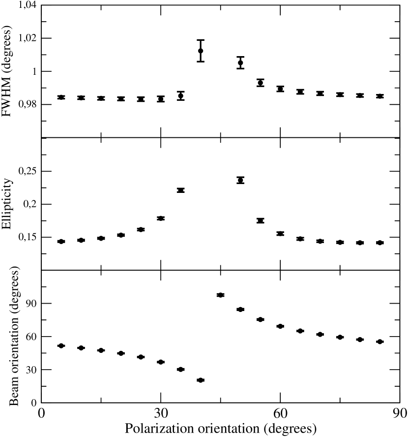
Figure 2.— Beam parameters computed from Tau A at K-band as a function of polarization orientation. Note that all uncertainties include statistical errors only, not systematic.

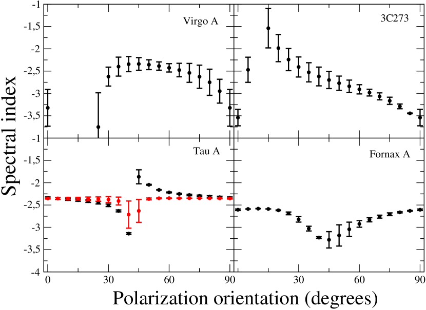
Figure 3.— Spectral index as a function of polarization angle for the four objects considered in this paper. The black points are computed from the K- and Ka-bands; the red points (for Tau A only) are computed from the Ka- and Q-bands.

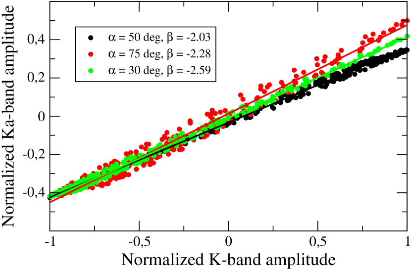
Figure 4.— TT plots for Tau A for three different polarization orientations. Note that the slopes are different for each direction, corresponding directly to different effective spectral indices. Further, there is no sign of either instrumental noise or background, demonstrating that the results are highly robust against such effects.

Observed ellipticity and FWHM

Although we smooth the data to a common angular resolution, and therefore should expect that the observations to have the desired FWHM, this is not true in practice due to beam asymmetries. To study the effective beam as a function of Stokes’ parameters, we rotate the original map by a rotation angle $\alpha$ into a new coordinate system $Q(\alpha)=Q\cos(2\alpha)+U\sin(2\alpha)$, and consider all angles between 0 and $90^{\circ}$ in steps of $5^{\circ}$. Then, in this new coordinate system we fit an elliptical Gaussian, $g(Q_{0},\textrm{FWHM},\epsilon,\psi)$, to the $Q$ signal by minimizing

$$\chi^{2}=\sum_{p}\left(\frac{Q_{p}(\alpha)-g(Q_{0},\textrm{FWHM},\epsilon,\psi)}{\sigma}\right)^{2},$$ (3)

where $Q_{0}$ is the source amplitude, $\epsilon$ is the ellipticity, and $\psi$ is the direction of the major semiaxis. (Note that it is sufficient to consider only the $Q$ component, because we rotate through all angles $\alpha$. Thus, $\alpha=45^{\circ}$ corresponds to $U$ in the original system.)

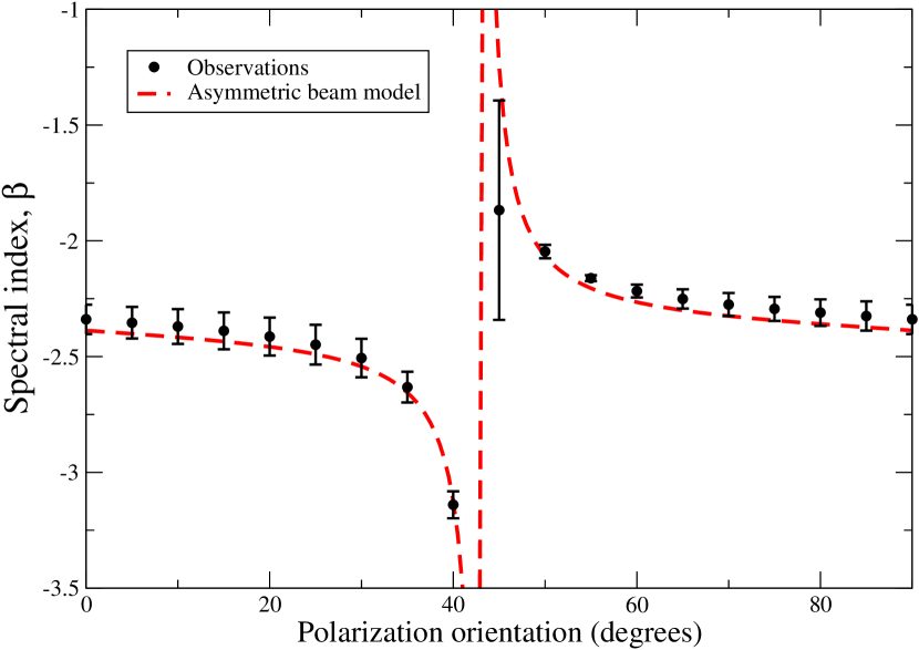
Figure 5.— Comparison of the observed (black points) and simulated (red line) spectral index for Tau A. The simulation is based on a noiseless point source observed with the same beam and polarization parameters as measured for Tau A. (See Tables 1 and 2 for full specification.)

Spectral indices

Finally, we estimate spectral indices for both $Q(\alpha)$ and $U(\alpha)$ using a standard TT-plot approach. For a single pixel with noiseless data, this approach is simply defined by

$$\frac{d_{\nu_{1}}(p)}{d_{\nu_{2}}(p)}=\left(\frac{\nu_{1}}{\nu_{2}}\right)^{\beta}\Rightarrow\beta=\frac{\log[d_{\nu_{1}}(p)/d_{\nu_{2}}(p)]}{\log[\nu_{1}/\nu_{2}]}.$$ (4)

However, for multiple noisy observations more robust results are obtained by fitting a straight line, $y=ax+b$, to $d_{\nu_{1}}$ as a function of $d_{\nu_{2}}$. An additional advantage of this method is its insensitivity to absolute offsets in the data. The spectral index is given as $\beta=\log a/\log(\nu_{1}/\nu_{2})$. Since both $d_{\nu_{1}}$ and $d_{\nu_{2}}$ have uncertainties, it is important to use a method that supports uncertainties in both directions with making the linear fit. In this paper, we adopt the approach described by Petrolini (2011). As in the case of the beam parameters, we also compute the spectral index as a function of polarization angle.

Table 2Polarization properties

	Polarization fraction		Polarization angle (degrees)		Spectral index
Object	K	Ka	K	Ka	$\beta_{T}$	$\beta_{P}$
Tau A	$6.17\pm 0.01$	$6.48\pm 0.04$	$88.43\pm 0.03$	$87.6\pm 0.1$	$-2.280\pm 0.001$	$-2.33\pm 0.01$
Virgo A	$3.4\pm 0.1$	$5.1\pm 0.8$	$-27\pm 1$	$-24\pm 4$	$-2.62\pm 0.01$	$-2.5\pm 0.3$
3C273	$5.8\pm 0.2$	$4.4\pm 0.6$	$52.7\pm 0.6$	$44\pm 2$	$-2.27\pm 0.01$	$-2.8\pm 0.2$
Fornax A	$6.7\pm 0.2$	$6.7\pm 0.5$	$-2.6\pm 0.7$	$-5\pm 2$	$-2.90\pm 0.02$	$-2.6\pm 0.2$

Note. — Uncertainties on polarization fraction and angles include only statistical errors; uncertainties on spectral indices additionally include an estimate of systematic errors.

Estimation of uncertainties for spectral indices is a non-trivial issue, because the inherent systematic errors turn out to be significantly larger than the statistical. We therefore add a systematic error term in quadrature to the statistical error. The systematic error is defined by splitting the observed data points in two sets, according to whether $d_{\nu_{1}}$ is larger or smaller than $ad_{\nu_{2}}+b$, and estimate a new slope for each set. The systematic error is taken to be the half difference between the two slopes.

4. Results

In Table 1 we list the position and apparent (beam-convolved) size and shape of each of the four objects under consideration. The polarization fraction and angles, and spectral indices are tabulated in Table 2. Images of Tau A are shown in Figure 1, both for K- (left column) and Ka-band (right column), and for Stokes’ $Q$ and $U$ parameters. In order to highlight the beam differences between these cases, we have first adopted a coordinate system which is offset by $22.5^{\circ}$ from the intrinsic polarization direction of Tau A. This ensures a significant signal-to-noise in both $Q$ and $U$. Second, the color scale is tuned to highlight the tails of the instrumental beam, and scaled properly between the two frequencies taking into account the spectral index of Tau A.

The main results of this paper are shown in Figures 2 and 3. The first figure shows the beam parameters for Tau A as a function of polarization orientation, and the second shows the spectral index as a function of polarization direction for all four sources. In the latter, the black points indicate the spectral index computed from K- and Ka-bands, and (for Tau A only) the red points show the spectral index between Ka- and Q-band. Figure 4 shows a subset of the Tau A TT plots that are used for the K-Ka calculations, corresponding to $\alpha=30^{\circ}$, $50^{\circ}$ and $75^{\circ}$, respectively.

As seen from the results shown in Figure 3, the polarized spectral index as measured by WMAP between K- and Ka-band at $1^{\circ}$ angular scale depends strongly on the coordinate system in which the index is computed. For Tau A, the derived index varies between, say, $\beta=-2.6$ for a rotation angle of $\alpha=30^{\circ}$ and $\beta=-2.0$ for $\alpha=50^{\circ}$. This effect is statistically highly significant, and it is robust with respect to instrumental noise and background levels (see Figure 4). It therefore indicates the presence of a real systematic effect not taken into account in the present analysis.

To understand these structures in greater detail, we construct an elliptical Gaussian model of Tau A based on the parameters listed in Tables 1 and 2 at K- and Ka-band, and estimate the spectral index from the resulting noiseless model, as for the real data. The results are shown in Figure 5. Clearly, the model faithfully reproduces the observed structures. The only difference is a slight vertical offset, which is due to the fact that the measured spectral index (reported in Table 2) is not a perfectly unbiased estimate of the true spectral index in the presence of systematics.

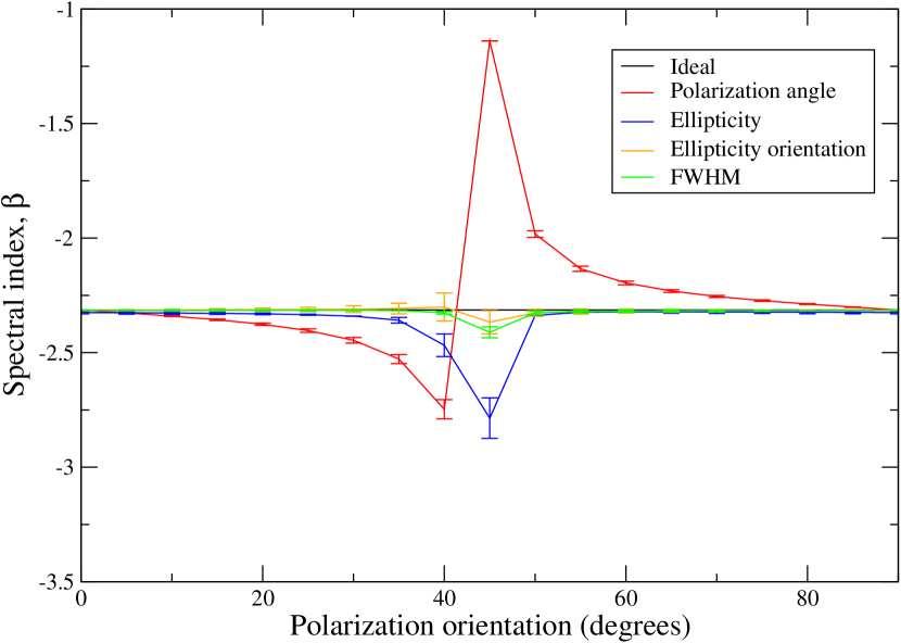
Figure 6.— The effect of various systematics on the measured spectral index of Tau A between K and Ka-band. The simulated K-band map is always based on the measured Tau A parameters. For the black curve we have used the same beam and polarization angle parameters for Ka as for K, corresponding to an ideal instrument. For the other curves we change one parameter at a time to the measured Ka value.

We can now use this model to understand the relative importance of the various systematic effects. To do so, we start out with an ideal model, adopting the observed K-band parameters also for Ka-band, and set the Ka parameters one-by-one to their true values. The results from this exercise are shown in Figure 6. Here we see that the most important systematic by far is the detector angle, and this effect alone reproduces the signal seen in Figure 5 very well. The second most important effect is the beam ellipticity, which is at least three to four times smaller than the detector angle effect over most of the well-sampled regions of the polarization orientation. Other effects are small compared to these two.

5. Conclusions

We have studied four particularly bright polarized point sources in the 7-year WMAP data, with the goal of understanding the effect of systematics on polarized spectral index estimation. This topic is important for at least two reasons. First, the WMAP polarization sky maps represents the best currently available full-sky measurements of the polarized foregrounds at CMB frequencies. As a result, they play a critical role in the analysis and optimization of existing and future B-mode experiments. Second, many ground-based and sub-orbital experiments use the WMAP polarization measurements of Tau A directly as a calibration source for both detector angles and absolute gain.

In this paper, we have found that the observed polarized spectral index of the relevant sources depends sensitively on the coordinate system in which the index is estimated. For example, the spectral index of Tau A is $\beta=-2.59\pm 0.03$ for a coordinate system rotated by $30^{\circ}$ relative to the intrinsic polarization direction of the source, while it is $\beta=-2.03\pm 0.01$ in a coordinate system rotated by $50^{\circ}$. The most significant contributor to this effect is the slightly different polarization angles of the K- and Ka-band detectors, with some smaller contribution coming from beam asymmetries. Experiments that, directly or indirectly, use the K- and Ka-band measurements of Tau A as a calibrator source should take into account these systematic uncertainties when performing their analyses.

Finally, we note that the test described in this paper is very simple to implement, only takes a few CPU seconds to run, and have a very direct and intuitive interpretation. We therefore expect other experiments to find it useful as a test of their own systematics, in particular when applied to Tau A.

References

- Aumont et al. (2010) Aumont, J., Conversi, L., Thum, C., et al. 2010, A&A, 514, A70
- Chiang et al. (2010) Chiang, H. C., Ade, P. A. R., Barkats, D., et al. 2010, ApJ, 711, 1123
- Dunkley et al. (2009) Dunkley, J., Spergel, D. N., Komatsu, E., et al. 2009, ApJ, 701, 1804
- Ekers et al. (1983) Ekers, R. D., Goss, W. M., Wellington, K. J., et al. 1983, A&A, 127, 361
- Fomalont et al. (1989) Fomalont, E. B., Ebneter, K. A., van Breugel, W. J. M., & Ekers, R. D. 1989, ApJ, 346, L17
- Gold et al. (2011) Gold, B., Odegard, N., Weiland, J. L., et al. 2011, ApJS, 192, 15
- Górski et al. (2005) Górski, K. M., Hivon, E., Banday, A. J.,Wandelt, B. D., Hansen, F. K., Reinecke, M., Bartelman, M. 2005, ApJ, 622, 759
- Jarosik et al. (2011) Jarosik, N., Bennett, C. L., Dunkley, J., et al. 2011, ApJS, 192, 14
- Liddle & Lyth (2000) Liddle, A. R., & Lyth, D. H. 2000, Cosmological Inflation and Large-Scale Structure, by Andrew R. Liddle and David H. Lyth, pp. 414. ISBN 052166022X. Cambridge, UK: Cambridge University Press, April 2000.
- Mitra et al. (2011) Mitra, S., Rocha, G., Górski, K. M., et al. 2011, ApJS, 193, 5
- Page et al. (2003) Page, L., Barnes, C., Hinshaw, G., et al. 2003, ApJS, 148, 39
- Petrolini (2011) Petrolini, A. 2011, [arXiv:1104.3132]
- QUIET (2011) QUIET collaboration 2011, ApJ, 741, 111
- QUIET (2012) QUIET collaboration 2012, ApJ, submitted, [arXiv:1207.5034]
- Rottmann et al. (1996) Rottmann, H., Mack, K.-H., Klein, U., & Wielebinski, R. 1996, A&A, 309, L19
- Wehus et al. (2009) Wehus, I. K., Ackerman, L., Eriksen, H. K., & Groeneboom, N. E. 2009, ApJ, 707, 343
- Weiland et al. (2011) Weiland, J. L., Odegard, N., Hill, R. S., et al. 2011, ApJS, 192, 19