Fidelity of a Rydberg blockade quantum gate from simulated quantum process tomography

Abstract

We present a detailed error analysis of a Rydberg blockade mediated controlled-NOT quantum gate between two neutral atoms as demonstrated recently in Phys. Rev. Lett. 104, 010503 (2010) and Phys. Rev. A 82, 030306 (2010). Numerical solutions of a master equation for the gate dynamics, including all known sources of technical error, are shown to be in good agreement with experiments. The primary sources of gate error are identified and suggestions given for future improvements. We also present numerical simulations of quantum process tomography to find the intrinsic fidelity, neglecting technical errors, of a Rydberg blockade controlled phase gate. The gate fidelity is characterized using trace overlap and trace distance measures. We show that the trace distance is linearly sensitive to errors arising from the finite Rydberg blockade shift and introduce a modified pulse sequence which corrects the linear errors. Our analysis shows that the intrinsic gate error extracted from simulated quantum process tomography can be under 0.002 for specific states of ⁸⁷Rb or Cs atoms. The relation between the process fidelity and the gate error probability used in calculations of fault tolerance thresholds is discussed.

I Introduction

Arrays of laser cooled neutral atoms in optical lattices or far-off-resonance optical traps (FORTs) are promising candidates for quantum computing experiments, due to their very long decoherence time (up to several seconds) for ground state atoms and strong two-atom interaction for highly excited Rydberg state atoms. This strong, long-range and controllable interaction leads to the so-called Rydberg blockade effect in which only one atom in an ensemble can be excited into a Rydberg state if the ensemble size is smaller than the Rydberg blockade radius. Jaksch et al. Jaksch et al. (2000) first proposed to use Rydberg blockade to implement a fast two-qubit controlled-phase gate (C_Z), which can be converted into a controlled-NOT gate (CNOT) using single qubit rotations Nielsen and Chuang (2000). Soon after, various schemes were proposed for fast quantum gates with an ensemble Lukin et al. (2001); Saffman and Walker (2005a); Isenhower et al. (2011); Wu et al. (2010), entangled state preparation Møller et al. (2008); *Muller2009; *Saffman2009b, quantum algorithms Chen (2011); Mølmer et al. (2011), quantum simulators Weimer et al. (2010); *Weimer2011, and efficient quantum repeaters Han et al. (2010); *Zhao2010.

Rydberg blockade, the central ingredient of the above schemes, has been demonstrated between two individual neutral atoms held in FORTs Urban et al. (2009); Gaëtan et al. (2009), and was used to demonstrate a two-qubit CNOT quantum gate Isenhower et al. (2010) and to generate entangled Bell states with fidelity of about $0.58-0.75$ after atom loss correction ($0.46-0.48$ without atom loss correction) Isenhower et al. (2010); Wilk et al. (2010); Gaëtan et al. (2010). Using an improved apparatus Zhang et al. (2010) a fidelity of $0.92$ for the CNOT probability truth table and $0.71$ for Bell state fidelity after atom loss correction ($0.71/0.58$ for the CNOT truth table/Bell state fidelity without atom loss correction) was demonstrated. These proof-of-principle results are promising but are still far from simple estimates of Rydberg gate errors at the level of $E\sim 10^{-3}$ predicted in Jaksch et al. (2000); Saffman and Walker (2005b).

The simple estimates are based on intrinsic errors associated with the atomic physics of the states used for Rydberg blockade. The essential intrinsic errors are the finite lifetime of Rydberg states and the finite strength of the Rydberg-Rydberg blockade interaction. In addition to intrinsic errors, experiments are sensitive to several different sources of technical error: spontaneous emission from an intermediate level in a two-photon excitation scheme, magnetic field fluctuations, pulse area errors, Doppler effects due to finite atomic temperature, etc.. We have previously estimated gate errors Saffman and Walker (2005b); Zhang et al. (2010) by treating each error source separately in the small error limit and adding them together. This provides a good estimate for small errors but it is unreliable for larger errors, as in the experiments, and does not provide a rigorous fidelity measure for the gate operation.

In this paper we present a more rigorous treatment by including all known error sources in a master equation for the density matrix evolution (optical Bloch equations). We dynamically track the density matrix evolution during the CNOT pulse sequence and then average the results over the computational input states for comparison with simple analytical estimates. We also extract a rigorous value for the gate fidelity using simulated quantum process tomography. The numerical results are in good agreement with analytical error estimates when technical errors are neglected, and with experimental results when technical errors are included in a Monte Carlo simulation. Numerical simulations of quantum process tomography with realistic atomic parameters confirm that it is in principle possible to reach quantum process errors of $2\times 10^{-3}$ for both Rb and Cs atoms.

In Sec. II we present the experimental setup and procedures used to demonstrate the CNOT gate and generate entangled Bell states. We also enumerate the various sources of technical imperfection in a realistic experiment. In Sec. III we give analytical estimates of the intrinsic gate error and present a new pulse sequence which removes the leading linear term in the finite blockade shift error. In Sec. IV we present a master equation model which includes both the technical error sources from II and intrinsic errors from Sec. III. In Sec. IV.1 we compare numerical Monte Carlo simulations with experimental results, and demonstrate good agreement. In Sec. IV.2 we perform simulated quantum process tomography of a two qubit controlled-phase gate accounting only for intrinsic errors. This analysis shows that in a well designed experiment where technical errors are minimized it should be possible to reach low gate errors, below known fault tolerance thresholdsKnill (2005); Raussendorf and Harrington (2007); *Aliferis2009; *Wang2011, for both Rb and Cs. A summary and discussion is presented in Sec. V.

II experimental procedures and technical imperfections

The experimental apparatus and procedures, as shown in Fig. 1, have been described in detail in our recent publications Isenhower et al. (2010); Zhang et al. (2010). For ease in understanding the subsequent analysis we include a brief description of the procedures, as well as estimates of various sources of technical imperfections.

II.1 Experimental procedures

We use FORTs to localize single ⁸⁷Rb atoms, which can be individually addressed using tightly focused beams that are scanned by acousto-optical modulators. The FORT beams, propagating along $+z$, are formed by focusing a laser beam with wavelength of $\lambda_{\rm f}=1064~{}\rm nm$ to a waist ($1/e^{2}$ intensity radius) of $w_{\rm f}=3.4~{}\mu\rm m$. We generate a linear array of trap sites using a diffractive element with the central site’s trap depth of $U_{0}/k_{B}=4.5~{}{\rm mK}$ and trap separation of about $9~{}\mu{\rm m}$ along the $x$ direction. We use two sites, one labeled as the control and the other as the target, to perform two-qubit quantum logic operations and to generate entangled states. A bias magnetic field is applied along $z$, which defines the quantization axis for the optical pumping ($B_{z}=0.15{\rm~{}mT}$) and lifts the degeneracy of the Zeeman sublevels ($B_{z}=0.37{\rm~{}mT}$) of Rydberg states during the gate operation. The relevant levels of ⁸⁷Rb are shown in Fig. 1b. We use the $5s_{1/2}$ hyperfine clock states as our qubits $|0\rangle\equiv|F=1,m_{F}=0\rangle$ and $|1\rangle\equiv|F=2,m_{F}=0\rangle$, separated by $\omega_{10}/2\pi=\mbox{6.83{\rm~{}GHz}}$, and the Rydberg state $|r\rangle\equiv|97d_{5/2},m_{j}=5/2\rangle$.

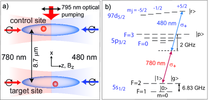
Figure 1: (color online) a) Experimental geometry. Two single atoms are trapped in two FORTs separated by about $9~{}\mu\rm m$. b) Relevant levels of ⁸⁷Rb. To reach the Rydberg state we use two-photon excitation with wavelengths of $780~{}\rm nm$ and $480~{}\rm nm$.

We perform single qubit rotations between $|0\rangle$ and $|1\rangle$ using two-photon stimulated Raman transitions driven by focusing a $\sigma_{+}$ polarized $780~{}\rm nm$ laser with frequency components separated by $\omega_{10}$ and detuned by $101{\rm~{}GHz}$ to the red of the D2 transition Yavuz et al. (2006). Total typical power in the two Raman sidebands is $\sim 90{\rm~{}}\mu{\rm W}$ with waist of $\omega_{x/y,g}=7.7{\rm~{}}\mu{\rm m}$, giving a single qubit Rabi frequency of $\Omega_{g}/2\pi=0.56{\rm~{}MHz}$ with $\pi$ pulse times of $\sim 900~{}\rm ns$ and peak-to-peak amplitude of better than 0.98 after correction for background atom loss of $10\%$ Zhang et al. (2010).

For coherent Rydberg excitation between $|1\rangle$ and $|r\rangle$ we use a two-photon transition with $\sigma_{+}$ polarized 780 and $480~{}\rm nm$ beams Johnson et al. (2008). They counter-propagate along the trap’s axial $z$ direction to minimize Doppler broadening of the transition. The $780~{}\rm nm$ beam is tuned about $2.0{\rm~{}GHz}$ to the red of the $|1\rangle\rightarrow|5p_{3/2},F^{{}^{\prime}}=3\rangle$ transition with typical beam power of $2.4{\rm~{}}\mu{\rm W}$ and waist of $\omega_{x/y,R}=7.7{\rm~{}}\mu{\rm m}$. The $480~{}\rm nm$ beam is tuned about $2.0{\rm~{}GHz}$ to the blue of the $|5p_{3/2},F^{{}^{\prime}}=3\rangle\rightarrow|r\rangle$ transition with typical beam power of $13~{}\rm mW$ and waist of $\omega_{x/y,B}=4.5{\rm~{}}\mu{\rm m}$. This gives a Rydberg red Rabi frequency of $\Omega_{\rm R}/2\pi=118{\rm~{}MHz}$, a Rydberg blue Rabi frequency of $\Omega_{\rm B}/2\pi=39{\rm~{}MHz}$, and Rydberg Rabi frequency of $\Omega/2\pi=1.15{\rm~{}MHz}$ with $\pi$ pulse times of $\sim 440~{}\rm ns$ and amplitude of 0.92 after correction for background atom loss of $10\%$.

In order to perform a two qubit CNOT gate we start by loading single atoms from a background vapor magneto-optical trap into two FORT sites. The trapped atoms have a measured temperature of $T_{\rm a}\simeq 175~{}\mu{\rm K}$ using a release and recapture method Reymond et al. (2003); *Tuchendler2008. Atom detection is accomplished by simultaneously illuminating both trapping sites with near resonant red-detuned molasses light, and imaging the fluorescence onto a cooled EMCCD camera. Detected photon counts are integrated for approximately 20 ms. Comparison of the integrated number of counts in a region of interest with predetermined thresholds indicates the presence or absence of a single atom Urban et al. (2009). After single atoms are loaded in these sites they are optically pumped into $|1\rangle$ with efficiency of about $99\%$ Zhang et al. (2010) using $\pi$ polarized light propagating along $-x$ tuned to the $|5s_{1/2},F=2\rangle\rightarrow|5p_{1/2},F^{{}^{\prime}}=2\rangle$ D1 transition at $795~{}\rm nm$ and $|5s_{1/2},F=1\rangle\rightarrow|5p_{3/2},F^{{}^{\prime}}=2\rangle$ D2 transition at 780 nm. This is followed by ground state $\pi$ pulses to either or both of the atoms to generate any of the four computational basis states. We then turn off the optical trapping potentials for about $4~{}\mu\rm s$, apply the CNOT pulses, and restore the optical traps. Ground state $\pi$ pulses are then applied to either or both atoms to select one of the four possible output states. Atoms left in state $|1\rangle$ are removed from the traps with unbalanced radiation pressure (blow away light), and a measurement is made to determine if the selected output state is present. The selection pulses provide a positive identification of all output states and we do not simply assume that a low photoelectron signal corresponds to an atom in $|1\rangle$ before application of the blow away light Isenhower et al. (2010); Zhang et al. (2010).

Following the above procedures we have obtained the CNOT truth table fidelity of $F=\frac{1}{4}{\rm Tr}[U_{{\rm ideal}}^{T}U_{{\rm CNOT}}]=0.92\pm 0.06$ with $U_{\rm ideal}$ and $U_{\rm CNOT}$ the ideal and experimentally obtained CNOT truth tables. To measure the state preparation fidelity, we use the same sequence but without applying the CNOT pulses. The computational basis states are prepared with an average fidelity of $F=0.97$.

To create entangled states we use $\pi/2$ pulses on the control atom to prepare the input states $|ct\rangle=\frac{1}{\sqrt{2}}(|0\rangle+i|1\rangle)|1\rangle$ and $|ct\rangle=\frac{1}{\sqrt{2}}(|0\rangle+i|1\rangle)|0\rangle$. Applying the CNOT to these states creates two of the Bell states $|B_{1}\rangle=\frac{1}{\sqrt{2}}(|00\rangle+|11\rangle)$ and $|B_{2}\rangle=\frac{1}{\sqrt{2}}(|01\rangle+|10\rangle$). In order to verify entanglement we measured the coherence of the $|B_{1}\rangle$ state by parity oscillations Isenhower et al. (2010); Zhang et al. (2010), and obtained a Bell state fidelity of $0.58$ without any atom loss correction ($0.71$ after correction) Zhang et al. (2010). Comparable numbers for the Bell state fidelity were obtained in a related experiment Wilk et al. (2010).

II.2 Technical imperfections

The main technical errors that affect the CNOT operation are spontaneous emission of the intermediate level during Rydberg excitation, magnetic noise, Doppler effects due to finite atom temperature and Rydberg laser power fluctuations.

The spontaneous emission error of the intermediate level during a $\pi$ excitation pulse can be estimated by $P_{\rm se}=\frac{\pi\gamma_{p}}{4|\Delta_{p}|}(|\frac{\Omega_{\rm R}}{\Omega_{\rm B}}|+|\frac{\Omega_{\rm B}}{\Omega_{\rm R}}|)$, with $\gamma_{p},\Delta_{p}$ the radiative linewidth and detuning from the $p$ level. This error is about $0.8\%$ for our current experimental setup.

Magnetic field fluctuations cause transition shifts, giving a Rydberg two-photon detuning $\Delta_{\rm B}=(g_{r}m_{r}-g_{1}m_{1})\mu_{B}B_{z}$ with $g_{r}=6/5$, $m_{r}=5/2$, $g_{1}=1/2$, and $m_{1}=0$ for our implementation in Fig. 1b). We assume that the magnetic field fluctuations are Gaussian distributed with a standard deviation of $\sigma_{\rm B}=2.5\times 10^{-6}~{}T$. This value was found by measuring the decoherence time of the hyperfine qubit at two different bias magnetic field strengthsSaffman et al. (2011). Doppler broadening at finite atom temperature $T_{\rm a}$, also gives two-photon detuning $\Delta_{\rm D}=(k_{R}-k_{B})v$ with averaged variances of $\sigma_{vx}^{2}=\sigma_{vy}^{2}=\sigma_{vz}^{2}=\frac{k_{B}T_{\rm a}}{m}$ for both control and target atoms.

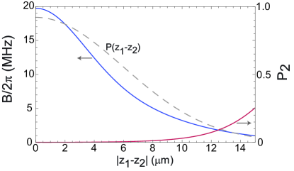
Figure 2: (color online) Calculated blockade shift $\sf B$ from the theory of Ref. Walker and Saffman (2008) and double excitation probability $P_{2}$ for state $|97d_{5/2},m_{j}=5/2\rangle$ as a function of relative position $P(|z_{1}-z_{2}|)$ for $0.37~{}\rm mT$ magnetic field. The relative probability distribution $P(|z_{1}-z_{2}|)$ assumes a trapping potential $U/k_{B}=4.5~{}{\rm mK}$, waist $w=3.4~{}\mu{\rm m}$ of the 1064 nm trapping light and atom temperature T$=175~{}\mu{\rm K}$.

Other technical errors associated with finite atom temperature are Rydberg blockade shifts, pulse area fluctuations, and AC Stark shifts (or two-photon detunings) due to the atomic position distribution in the FORTs. We assume that the atomic position distribution for both control and target atoms is Gaussian with variance of Saffman and Walker (2005b) $\sigma_{x}^{2}=\sigma_{y}^{2}=\frac{w_{f}^{2}}{4}\frac{k_{B}T_{\rm a}}{U_{0}}$ and $\sigma_{z}^{2}=\frac{\pi{}^{2}w_{\rm f}^{4}}{2\lambda_{\rm f}^{2}}\frac{k_{B}T_{\rm a}}{U_{0}}$. For the Rydberg blockade shift due to the atomic position distribution, we use the theoretical blockade shift curve as a function of relative atomic separation $|z_{1}-z_{2}|$ as shown in Fig. 2. The position dependent Rabi frequency and AC Stark shifts are

$$\Omega_{\rm R}({\bf r}) = \Omega_{\rm R}(0)\frac{e^{-\left[\frac{x^{2}}{w_{x,R}^{2}\left(1+z^{2}/L_{x,R}^{2}\right)}+\frac{y^{2}}{w_{y,R}^{2}\left(1+z^{2}/L_{y,R}^{2}\right)}\right]}}{[(1+z^{2}/L_{x,R}^{2})(1+z^{2}/L_{y,R}^{2})]^{1/4}}$$

$$\Omega_{\rm B}({\bf r}) = \Omega_{\rm B}(0)\frac{e^{-\left[\frac{x^{2}}{w_{x,B}^{2}\left(1+z^{2}/L_{x,B}^{2}\right)}-\frac{y^{2}}{w_{y,B}^{2}\left(1+z^{2}/L_{y,B}^{2}\right)}\right]}}{[(1+z^{2}/L_{x,B}^{2})(1+z^{2}/L_{y,B}^{2})]^{1/4}}$$

and

$$\Delta_{\rm AC}({\bf r})=\Delta_{\rm AC}(0)+\frac{\Omega_{\rm R}^{2}({\bf r})-\Omega_{\rm B}^{2}({\bf r})}{4|\Delta_{p}|}.$$ (3)

Here $\Omega_{\rm R}(0)$, $\Omega_{\rm B}(0)$, and $\Delta_{\rm AC}(0)$ are the Rydberg red, blue and AC Stark shifts at trap center, respectively; the Rayleigh lengths are $L_{x/y,R}=\pi w_{x/y,R}^{2}/\lambda_{\rm R}$ and $L_{x/y,B}=\pi w_{x/y,B}^{2}/\lambda_{\rm B}$.

Power fluctuations of the Rydberg lasers will not only affect the Rabi frequencies $\Omega_{\rm R}$ and $\Omega_{\rm B}$, but will also affect the two photon detuning $\Delta_{\rm AC}$. We assume that the power fluctuations of the red and blue lasers are both Gaussian distributed with FWHM of $1\%$ and $2\%$, respectively, as measured independently.

II.3 Dephasing errors

The technical imperfections listed in the previous section show up as errors in the measured CNOT probability truth table as well as in the fidelity of the output quantum states. There are additional technical dephasing errors that do not significantly affect the CNOT truth table but strongly impact the fidelity of Bell state generation. As was pointed out in Refs. Wilk et al. (2010); Saffman et al. (2011) both magnetic field fluctuations and atomic motion lead to dephasing of the Rydberg state relative to the ground state during gate operation because the motion of Rydberg atoms between excitation and deexcitation pulses leads to a stochastic phase that degrades the entanglement. In the numerical simulations described in Sec. IV we do not keep track of the position dependent phase of the optical fields in the evolution Hamiltonians during each blockade pulse sequence(Eqs. (14l) and (15g) below) . Instead we add an extra dephasing term $\gamma_{\rm ph}$ to the Liouville operators of Eqs. (14l) and (15n) in Sec. IV:

$$\gamma_{\rm ph}=\sqrt{(\gamma_{\rm B})^{2}+(\gamma_{\rm D})^{2}},$$ (4)

where $\gamma_{\rm B}=|\Delta_{\rm B}|/\hbar$ and $\gamma_{\rm D}=\Delta_{\rm D}$ are the dephasing rates due to magnetic field fluctuations and Doppler effects, respectively. In the Monte Carlo simulations presented below these dephasing rates are sampled from distributions that are generated with the position and velocity variances described above. Both the magnetic field fluctuations and atom position variations at finite temperature also dephase the qubit states by varying the hyperfine splitting between them. We model the qubit dephasing as

$$\gamma_{01}=\sqrt{(\gamma_{B01})^{2}+(\gamma_{T})^{2}}$$ (5)

where $\gamma_{B01}=\omega_{10}(B_{z}+\sigma_{\rm B})-\omega_{10}(B_{z})$, is the dephasing rate due to the second-order Zeeman shift of the clock transition by magnetic field fluctuations, $B_{z}$ is a static bias field, $\omega_{10}(B_{z})=\omega_{10}\sqrt{1+\left[\frac{(g_{S}-g_{I})\mu_{B}B_{z}}{\hbar\omega_{10}}\right]^{2}}$ is the ground hyperfine splitting of the clock states, $g_{S},g_{I}$ are electron and nuclear Landé factors, and $\sigma_{B}$ is the magnetic field fluctuation; $\gamma_{T}=1.03\frac{\delta_{0}k_{B}T_{\rm a}}{2U_{0}}$ Saffman and Walker (2005b); Kuhr et al. (2005), is the dephasing rate in 1/ms due to atomic motion in the FORT, $U_{0}$ is the peak FORT potential, $\delta_{0}/2\pi=(U_{0}/k_{B})\times(1.5~{}\rm kHz/mK)$, is the peak differential light shift of the FORT and $T_{\rm a}$ is the atom temperature.

In addition to the above errors, there are also errors associated with state preparation due to imperfect optical pumping and single qubit rotations. These errors are at about the $1\%$ level. There is also about $1\%$ atom loss due to background collisions before the CNOT pulse sequence.

III Intrinsic error estimates

Even if all sources of technical error described in Sec. II.2 are negligible there will still be intrinsic gate errors due to the basic physics of the Rydberg blockade interaction. Intrinsic errors of a Rydberg blockade CNOT gate include the decoherence error due to the finite lifetime $\tau$ of the Rydberg state and rotation errors due to imperfect blockade. In the strong blockade limit ($\Omega\ll{\sf B}\ll\omega_{10}$, where $\sf B$ is the Blockade shift), the intrinsic gate error $E_{1}$ averaged over the input states in the computational basis $(\{|00\rangle,|01\rangle,|10\rangle,|11\rangle\})$ is Saffman and Walker (2005b); Saffman et al. (2010)

$$E_{1}=\frac{7\pi}{4\Omega\tau}\left(1+\frac{\Omega^{2}}{\omega_{10}^{2}}+\frac{\Omega^{2}}{7{\sf B}^{2}}\right)+\frac{\Omega^{2}}{8{\sf B}^{2}}\left(1+6\frac{\Omega^{2}}{\omega_{10}^{2}}\right)$$ (6)

The first term in Eq. (6) is the Rydberg decay error due to the finite lifetime $\tau$ of the Rydberg state, and the second term is the imperfect blockade error. In the limit of $\omega_{10}\gg({\sf B},\Omega)$ we can extract a simple expression for the optimum Rabi frequency which minimizes the error

$$\Omega_{1_{\rm opt}}=(7\pi)^{1/3}\frac{{\sf B}^{2/3}}{\tau^{1/3}}.$$ (7)

Setting $\Omega\rightarrow\Omega_{1_{\rm opt}}$ leads to a minimum averaged gate error of

$$E_{1_{\rm min}}=\frac{3(7\pi)^{2/3}}{8}\frac{1}{({\sf B}\tau)^{2/3}}.$$ (8)

In our experiments $\tau\sim 300{\rm~{}}\mu{\rm s}$ is the radiative lifetime of the $97d_{5/2}$ Rydberg level, $\omega_{10}/2\pi=6.83~{}{\rm GHz}$, and $\Omega/2\pi=1.15~{}{\rm MHz}$. In the experimental geometry shown in Fig. 1a) a range of two-atom separations, and hence blockade shifts, occur. The blockade shift curve shown in Fig. 2 is calculated from the theory of Ref. Walker and Saffman (2008) using a trap separation of $x=8.7~{}\mu{\rm m}$ and a bias magnetic field of $B_{z}=0.37~{}{\rm mT}$ applied along the $\hat{z}$ axis. Averaging Eq. (6) over the probability distribution P$(|z_{1}-z_{2}|)$, which is dependent on the trapped atom temperature of $175~{}\mu{\rm K}$, gives an expected error of $E=8.5\times 10^{-3}$. The corresponding averaged blockade shift from Eq. (6) is $\bar{\sf B}/2\pi=5.3~{}{\rm MHz}$.

It should be emphasized that the average error $E_{1}$ discussed above ignores errors in the phases of the states generated by the CNOT gate and therefore corresponds to the measurement of a probability truth table. As discussed in Ref. Jaksch et al. (2000), a Rydberg-mediated C_Z gate has a phase error for the $|11\rangle$ input state of $|11\rangle\rightarrow-e^{\imath\phi}|11\rangle$ with $\phi=\pi\Omega/2{\sf B}$. Averaging over the four computational basis states gives an average intrinsic phase error of $E_{\phi}=\pi\Omega/8{\sf B}$. Including the phase error, we find an average intrinsic gate error of

$$E_{2}=E_{1}+\frac{\pi\Omega}{8{\sf B}}.$$ (9)

When $\Omega\ll{\sf B}$ the last term in Eq. (9), dominates over the imperfect blockade term in Eq. (6). Using Eq. (9) we can again extract a simple expression for the optimum Rabi frequency which minimizes the error

$$\Omega_{2_{\rm opt}}=\left(\frac{14{\sf B}}{\tau}\right)^{1/2}.$$ (10)

Setting $\Omega\rightarrow\Omega_{2_{\rm opt}}$ leads to a minimum averaged gate error of

$$E_{2_{\rm min}}=\frac{\sqrt{7}\pi}{2\sqrt{2}}\frac{1}{({\sf B}\tau)^{1/2}}.$$ (11)

Comparing Eqs. (8) and (11) in the experimentally relevant limit of ${\sf B}\tau\gg 1$ we see that $E_{2_{\rm min}}\gg E_{1_{\rm min}}$. This result seems to imply that Eq. (8) provides an overly optimistic estimate for the gate error.

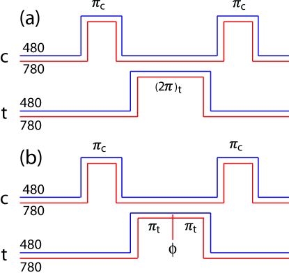
Figure 3: (color online) Pulse sequence for Rydberg C_Z gate with two-photon 780 and 480 nm excitation of Rb atoms followingJaksch et al. (2000) a) and modified sequence to correct finite blockade phase error by rapidly changing the phase of one of the Rydberg beams by $\phi$ b).

Despite this apparently disappointing result the gate error can indeed be made to satisfy the $({\sf B}\tau)^{-2/3}$ scaling of Eq. (8) by a modification of the C_Z sequence as shown in Fig. 3b). We note that the only input state for which the target atom becomes Rydberg excited is $|01\rangle$. By shifting the phase of the $|5p_{3/2}\rangle\rightarrow|r\rangle$ laser used for Rydberg excitation by an amount $\phi$ during the gate operation we can add a phase of $\phi$ to this state. This results in a phase gate

$$C_{Z}=\left(\begin{array}[]{cccc}1&0&0&0\\ 0&-e^{\imath\phi}&0&0\\ 0&0&-1&0\\ 0&0&0&-e^{\imath\phi}\end{array}\right).$$ (12)

Adding a single qubit $Z$ rotation of $-\phi$ to the control atom cancels the extra phases, leaving an ideal C_Z operation. As we show in detail in Sec. IV.2 using simulated process tomography, the standard sequence of Fig. 3a gives linear phase errors that impact the trace distance fidelity measure. Using the modified pulse sequence the linear phase errors are canceled and the trace distance error is reduced.

We emphasize that perfect correction of the phase error using this modified gate sequence assumes that ${\sf B}$, and therefore the phase $\phi$, are well defined, and do not fluctuate. This is not true for thermally excited atoms but will be the case for atoms that are in the motional ground state of the confining potentials. If the atoms are thermally excited we can still cancel the average value of $\phi$, but errors due to fluctuations about the average would remain. In the analysis of the intrinsic error limit we assume that the atoms are in the motional ground state so the phase can be canceled exactly.

IV numerical simulations

In order to accurately simulate the performance of the Rydberg gate we integrate the master equation for the two-atom dynamics including all known coherent and incoherent rates. A related analysis was performed previously for the Rydberg excitation dynamics of a single atom Miroshnychenko et al. (2010). For each atom we include five atomic states in our numerical calculation, which are labeled in the level scheme of Fig. 1b): qubit $|0\rangle$, qubit $|1\rangle$, and reservoir level $|g\rangle\equiv|{5s}_{1/2},m_{F}\neq 0\rangle$ in the ${5s}_{1/2}$ ground state; the intermediate level $|p\rangle\equiv|5p_{3/2}\rangle$ and the Rydberg level $|r\rangle$. With this set of basis states the two-atom dynamics are described by density matrices $\rho_{\rm ct}(t)$ with dimensions $25\times 25$. We take the initial condition to be a separable state $\rho_{\rm ct}(0)=\rho_{\rm c}(0)\otimes\rho_{\rm t}(0)$, with c/t for control/target atoms. We calculate the time evolution by solving the master equation

$$\frac{d\rho_{\rm ct}}{dt}=-\frac{i}{\hbar}[H_{\rm ct},\rho_{\rm ct}]+\mathcal{L_{\textrm{ct}}},$$ (13)

with ${H}_{\rm ct}={H}_{\rm c}\otimes I_{\rm t}+I_{\rm c}\otimes{H}_{\rm t}+\hbar{\sf B}\left[\begin{array}[]{cc}0_{24}&0\\ 0&1\end{array}\right]$, $\mathcal{L}_{\rm ct}=\mathcal{L}_{\rm c}\otimes I_{\rm t}+I_{\rm c}\otimes\mathcal{L}_{\rm t}$, $I_{\rm t}$ $(I_{\rm c})$ are $5\times 5$ identity matrices, and 0₂₄ is a $24\times 24$ zero matrix. The Hamiltonian ${H}_{\rm c}$ (${H}_{\rm t}$), after making the rotating-wave approximation, and the Liouville operators $\mathcal{L_{\textrm{c}}}$ ($\mathcal{L_{\textrm{t}}}$) are given in the basis $\{|0\rangle,|g\rangle,|1\rangle,|p\rangle,|r\rangle$} as

$${H_{\rm(c/t)}} = \hbar\left(\begin{array}[]{ccccc}-\omega_{10}&0&0&\Omega_{\rm R(c/t)}^{*}/2&0\\ 0&0&0&0&0\\ 0&0&0&\Omega_{\rm R(c/t)}^{*}/2&0\\ \Omega_{\rm R(c/t)}/2&0&\Omega_{\rm R(c/t)}/2&\Delta_{p}&\Omega_{\rm B(c/t)}^{*}/2\\ 0&0&0&\Omega_{\rm B(c/t)}/2&\Delta_{\rm r}\end{array}\right),$$ (14f)

$$\mathcal{L} = \left(\begin{array}[]{ccccc}0.12\gamma_{p}\rho_{pp}&0&-\frac{\gamma_{01}}{2}\rho_{01}&-\frac{\gamma_{p}}{2}\rho_{0p}&-\frac{\gamma_{r}}{2}\rho_{0r}\\ 0&0.56\gamma_{p}\rho_{pp}&0&-\frac{\gamma_{p}}{2}\rho_{gp}&-\frac{\gamma_{r}}{2}\rho_{gr}\\ -\frac{\gamma_{01}}{2}\rho_{10}&0&0.32\gamma_{\rm p}\rho_{pp}&-\frac{\gamma_{p}}{2}\rho_{1p}&-\frac{\gamma_{1r}}{2}\rho_{1r}\\ -\frac{\gamma_{p}}{2}\rho_{p0}&-\frac{\gamma_{p}}{2}\rho_{pg}&-\frac{\gamma_{p}}{2}\rho_{p1}&-\gamma_{p}\rho_{pp}+\gamma_{r}\rho_{rr}&-\frac{\gamma_{p}+\gamma_{r}}{2}\rho_{pr}\\ -\frac{\gamma_{r}}{2}\rho_{r0}&-\frac{\gamma_{r}}{2}\rho_{rg}&-\frac{\gamma_{1r}}{2}\rho_{r1}&-\frac{\gamma_{p}+\gamma_{r}}{2}\rho_{rp}&-\gamma_{r}\rho_{rr}\end{array}\right).$$ (14l)

For Rb atoms we take into account the spontaneous emission from the intermediate level $|p\rangle$ to the ground level with a decay rate of $\gamma_{p}/2\pi=6.07~{}{\rm MHz}$ and the corresponding branching ratio of 0.56 to state $|g\rangle$, 0.32 to state $|1\rangle$ and 0.12 to state $|0\rangle$ as well as the decay from the Rydberg state $|r\rangle$ to the intermediate level $|p\rangle$ with rate $\gamma_{r}/2\pi=0.53~{}{\rm kHz}$. $\Delta_{p}$ is the intermediate level detuning, $\Delta_{{r}}=\Delta_{\rm AC}({\bf r})+\Delta_{\rm B}+\Delta_{\rm D}$ is the two photon detuning (see Sec. II.2), $\omega_{10}/2\pi=6.83~{}{\rm GHz}$ is the hyperfine ground state splitting; $\gamma_{1r}=\gamma_{r}+\gamma_{\rm ph}$ is the total dephasing of the Rydberg state relative to $|1\rangle$, $\gamma_{\rm ph}$ is the Rydberg dephasing rate due to magnetic field fluctuations and Doppler effects as shown in Eq. (4); and $\gamma_{01}$ is the dephasing of qubit states due to magnetic field fluctuations and atomic motion.

Note that we do not include driving terms in Eq. (14l) that couple the reservoir level $|g\rangle$ back to $|p\rangle$ and $|r\rangle$. Doing so correctly would require adding additional Rydberg levels with different values of $m_{j}$ which would increase the numerical burden. Since any population in $|g\rangle$ is already fully counted as an error, including additional driving terms would only reduce the final errors, and our results are reliably upper bounds on the gate error.

Table 1: Experimental parameters used in Ref. Zhang et al. (2010) as well as in the numerical simulations.

Experimental parameter	symbol	value
FORT wavelength	$\lambda_{f}$	$1064~{}{\rm nm}$
FORT waist	$w_{x,y}$	$3.4~{}\mu{\rm m}$
FORT trap depth	$U_{0}/k_{B}$	$4.5~{}\rm mK$
FORT separation	$d$	8.7 $\mu\rm m$
Atom temperature	$T_{\rm a}$	$175~{}\mu\rm K$
Rydberg level	$|r\rangle$	$97d_{5/2}$
Rydberg state radiative lifetime	$\tau$	$320~{}\mu{\rm s}$
Blockade shift at $0~{}\mu{\rm K}$	${\sf B}_{0}/2\pi$	$20~{}\rm MHz$
Rydberg red power		$2.4~{}\mu\rm W$
Rydberg red waist	$w_{x/y,R}$	$7.7~{}\mu{\rm m}$
Rydberg red detuning	$\Delta_{p}/2\pi$	$-2~{}\rm GHz$
Rydberg blue power		$13~{}\rm mW$
Rydberg blue waist	$w_{x/y,B}$	$4.5~{}\mu{\rm m}$
Rydberg red Rabi frequency	$\Omega_{\rm R}/2\pi$	$118~{}\rm MHz$
Rydberg blue Rabi frequency	$\Omega_{\rm B}/2\pi$	$39~{}\rm MHz$
Rydberg Rabi frequency	$\Omega/2\pi$	$1.15~{}\rm MHz$
Magnetic field fluctuation	$\sigma_{\rm B}$	$2.5~{}\mu\rm T$
Rydberg red power fluctuation		1%
Rydberg blue power fluctuation		2%

IV.1 Monte Carlo Simulations including technical errors

In our numerical calculation, we consider two traps aligned along $z$ with separation of $8.7~{}\mu{\rm m}$ as shown in Fig. 1a). The atoms in each trap have temperature $T_{\rm a}$ and Gaussian spatial probability distribution with variances of $\sigma_{x}$ , $\sigma_{y}$, and $\sigma_{z}$ as given in Sec. II.2. Rydberg Rabi pulses are applied to the control or target atoms with Gaussian power fluctuations of FWHM of $1\%$ and $2\%$ for Rydberg red and blue lasers, respectively. An atom at position ${\bf r}=(x,y,z)$ with velocity ${\bf v}=(v_{x},v_{y},v_{z})$ experiences a Rydberg excitation pulse with effective Rabi frequency and two-photon detuning that depends on position and velocity, so $\Omega=\Omega({\bf r})$ and $\Delta_{r}=\Delta_{r}({\bf r},{\bf v})$ as described in Sec. II.2. We also use a fit to the blockade curve of Fig. 2 to account for variations in the two-atom interaction strength. Finally we can monitor the effect of various error sources by switching them on and off and comparing the numerical results.

Numerical simulation of the CNOT gate demonstrated in Ref. Zhang et al. (2010) proceeds as follows. We start with the initial density matrix for both atoms with population of $0.98$ in either $|1\rangle$ or $|0\rangle$ and population of $0.02$ in $|g\rangle$ to account for an optical pumping error of $1\%$ and atom loss of $1\%$ before the CNOT pulses. Then we perform Monte Carlo simulations of the experiment with the actual experimental parameters from Ref. Zhang et al. (2010) as listed in Table 1. Next, we solve the time evolution of the master equation (13) for the $C_{Z}$ pulse sequence of Fig. 3a with $\pi/2$ pulses on the target atom before and after the $C_{Z}$ to give a CNOT operation: $\{(\frac{\pi}{2})_{\rm t},\pi_{\rm c},t_{\rm gap},(2\pi)_{\rm t},t_{\rm gap},\pi_{\rm c},(\frac{\pi}{2})_{\rm t}\}$ as in Zhang et al. (2010) and average over the four input states ($|00\rangle$, $|01\rangle$, $|10\rangle$ and $|11\rangle$) to get the averaged gate errors, where $(\frac{\pi}{2})_{\rm t}$ is a ground Raman $\pi/2$ pulse on the target atom, and $t_{\rm gap}=500~{}\rm ns$ is the switching time between control and target atom sites. Here, we treat the ground Raman pulse as an ideal unitary operation since it is substantially less sensitive to the various error sources than operations involving Rydberg states.

Table 2: CNOT probability truth table and entanglement fidelity results. The upper section of the table gives error budget values used in the numerical simulations. These values are based on laboratory measurements and theoretical estimates as described in Zhang et al. (2010). The lower section gives measured results from Zhang et al. (2010) and numerical values from solving Eq. (13).

	error
Parameter used in numerical simulation	budget
Optical pumping	0.02
Atom loss before CNOT pulses	0.02
Spontaneous emission	0.018
Rydberg decay error	0.003
Blockade error at $0~{}\mu{\rm K}$	0.0004
Blockade error at $175~{}\mu{\rm K}$	0.006
Doppler Broadening at $175~{}\mu{\rm K}$	0.003
Laser power fluctuation	0.0001
Magnetic field fluctuation	0.0002
	measured	numerical
	results	simulation
Background loss (two atoms)	0.19
CNOT trace loss ($1-{\rm Tr}[\rho_{\rm ct}]$)	0.01
CNOT probability truth table
raw fidelity	0.74	0.75
background loss corrected	0.91	0.93
background & trace corrected	0.92	0.93
Bell state
raw fidelity	0.58	0.54
background loss corrected	0.71	0.67
background & trace corrected	0.71	0.67

The probability truth table error is defined by $E=1-{\rm Tr}[\rho_{\rm ideal}^{T}\rho_{\rm ct}]$, where $\rho_{\rm ct}$ is the numerical simulation result. We should point out that the switching time $t_{\rm gap}$ is short enough that it has little effect on the CNOT truth table fidelity, but has a strong effect on the entanglement fidelity because the motion of Rydberg excited atoms between excitation and deexcitation pulses leads to a stochastic phase that degrades the entanglement as was pointed out in Wilk et al. (2010). Finally, we average over 100 evolutions of the master equation, and the final results are shown in Table 2.

To model the entanglement, we prepare the control atom in state $|c\rangle=\frac{1}{\sqrt{2}}(|0\rangle+i|1\rangle)$ and target atom in state $|t\rangle=|1\rangle$. Then we follow the same approach as for the CNOT truth table error analysis by solving the time evolution of the master equation (13). From the final density matrix after the pulse sequence, we can extract the Bell state fidelity $F$ defined as $F={\rm Tr}[\rho_{\rm ideal}^{T}\rho_{\rm ct}]$, where $\rho_{\rm ideal}$ is associated with the maximally entangled Bell state $|B_{1}\rangle=\frac{1}{\sqrt{2}}(|00\rangle+|11\rangle)$. We then average over 50 evolutions of the master equation using Monte Carlo simulation of all the error sources as mentioned before, and obtain the final Bell state fidelity $F=0.54$ without atom loss correction and fidelity $F=0.67$ after atom loss correction as shown in Table 2, which is consistent with our measured entangled fidelity of 0.71 in Zhang et al. (2010). We assume that the atom loss due to collisions with untrapped background atoms is independent of the CNOT pulse sequence (about $4~{}\mu{\rm s}$) which is much shorter than the trap lifetime (several seconds), so the background loss is simply considered as a scaling factor for the final fidelity without atom loss.

In Figure 4, we compare the numerical simulation results for the CNOT probability truth table with the analytical results of Eq. (6) for different parameters. Both the decoherence error $E_{\tau}$ (the first term in Eq. (6)) and imperfect blockade error $E_{B}$ (the second term in Eq. (6)) agree well with the numerical results in the small gate error limit. The total gate error with all the error sources is $6.5\%$ in agreement with the atom loss corrected fidelity of $F=0.92$ and the simple gate error analysis reported in Zhang et al. (2010). As shown in Table 2, the two main error sources limiting the gate fidelity are the spontaneous emission from state $|p\rangle$ and imperfect Rydberg excitation and blockade due to finite atomic temperature (not accounting for the atom loss before the CNOT pulses, the imperfect optical pumping and other losses that are independent of the CNOT pulse sequence).

The comparison of Monte Carlo master equation simulations with experimental data shows that the error sources listed in Table 2 are able to account for measured results with an accuracy of about 1% as regards the CNOT truth table and about 5% as regards the Bell state fidelity. The Bell state fidelity is much lower than that of the CNOT truth table due to dephasing that occurs while the control atom is Rydberg excited. As has been discussed in Wilk et al. (2010); Saffman et al. (2011) the main sources of the Rydberg dephasing are magnetic field noise and Doppler effects. In order to significantly reduce these errors it will be necessary to work with colder atoms, less magnetic field noise, and faster Rydberg excitation pulses.

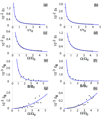
Figure 4: (color online) Comparison between intrinsic gate errors from Eq. (6) for different parameters and numerical simulations. In the first column (a, c, e, g): ${\sf B}_{0}/2\pi=10~{}{\rm MHz}$, $\Omega_{0}/2\pi=1.15~{}{\rm MHz}$, $\tau_{0}=300~{}\mu s$; in the second column (b, d, f, h): ${\sf B}_{0}/2\pi=10~{}{\rm MHz}$, $\Omega_{0}/2\pi=0.575~{}{\rm MHz}$, $\tau_{0}=300~{}\mu s$. $E_{\tau}$ is the decoherence error due to finite Rydberg lifetime (the first term in Eq. (6)) and $E_{B}$ is the imperfect blockade error (the second term in Eq. (6)). The black dotted points are the results of the numerical simulations and the blue lines are the results from Eq. (6) with the same parameters.

IV.2 Simulated Quantum Process Tomography

The experimental results obtained to date from Rydberg blockade experiments on pairs of atoms are far from predicted error thresholds for a practical fault-tolerant quantum computer which range from $10^{-4}-10^{-2}$ in different models Knill (2005); Raussendorf and Harrington (2007); *Aliferis2009; *Wang2011. In order to characterize more completely the fidelity and usefulness of Rydberg blockade for quantum computing applications we need to perform Quantum Process Tomography (QPT) Chuang and Nielsen (1997); *Poyatos1997; Nielsen and Chuang (2000) of the Rydberg blockade mediated quantum blackbox process. QPT has been demonstrated with several different physical systems including linear optics O’Brien et al. (2004); *White2007, trapped ions Riebe et al. (2006); *SXWang2010, and superconducting circuits Yamamoto et al. (2010); *Bialczak2010. Here, we perform numerical simulations of QPT with maximum likelihood estimation of tomographically reconstructed density matrices O’Brien et al. (2004); White et al. (2007) for the Rydberg-blockade $C_{Z}$ gate. We limit the simulations of intrinsic errors to the simpler $C_{Z}$ gate since it has been demonstratedOlmschenk et al. (2010); *Brown2011 that the additional single qubit pulses needed to implement a CNOT can be performed with errors at the $\sim 10^{-4}$ level.

Since our goal is to determine the minimum possible gate error that can be reached using Rydberg blockade we only account for intrinsic gate errors as described in Sec. III, and assume all additional technical errors are negligible. This corresponds to a situation where the atoms are cooled to their motional ground state so there is no Doppler dephasing during Rydberg excitation, position dependent variations in Rabi frequencies, or AC Stark shifts. We assume there is no spontaneous emission from the intermediate $|p\rangle$ level during Rydberg excitation. This could be achieved using one photon excitation of Rydberg $|p\rangle$ states, or by using sufficient laser power to detune very far from the intermediate $|p\rangle$ level. We also assume that dephasing due to time varying magnetic fields is negligible.

Accounting only for intrinsic gate errors the analytical estimates of Sec. III show that $E\sim({\sf B}\tau)^{-2/3}.$ At room temperature the Rydberg lifetime scales as $\tau\sim n^{2}$ with $n$ the principal quantum number and in the heavy alkali atoms Rb and Cs the van der Waals Blockade interaction scales asSaffman and Mølmer (2008) ${\sf B}\sim n^{12}$. Thus we expect the gate error to scale as $E\sim n^{-28/3}$ so that choosing large $n$ should give arbitrarily small errors.

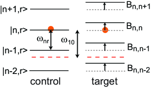
Figure 5: (color online) Level diagram accounting for neighboring Rydberg levels of control and target atoms. The Rydberg laser is tuned to excite $|1\rangle$ to $|n,r\rangle$. The red dashed lines show the energy that qubit state $|0\rangle$ is excited to, and ${\sf B}_{n,n^{\prime}}$ is the positive blockade shift between a control atom in $|nr\rangle$ and target atom in $|n^{\prime}r\rangle$.

This argument breaks down when $n\stackrel{{\scriptstyle>}}{{\sim}}100$ since the energy spacing of levels $n$ and $n\pm 1$ becomes comparable to ${\sf B}$ or $\omega_{10},$ as shown in Fig. 5. This puts a limit on the effective blockade shift that can be achieved at large $n$ and limits the error floor. For the $C_{Z}$ pulse sequence acting on the four possible input states in the computational basis $\{|00\rangle,|01\rangle,|10\rangle,|11\rangle\}$ excitation is blocked three times due to $\omega_{10}$, once due to $\omega_{10}+{\sf B}$ and once due to ${\sf B}$ alone. It is necessary to choose the Rydberg level spacing and blockade shift such that the excitation suppression is as large as possible for all three cases. The above description is valid for Rydberg $p_{3/2}$ and $d_{5/2}$ states since by using $\sigma_{+}$ polarized light the qubit states are only coupled to these Rydberg states gat . For $s_{1/2}$ states the situation is worse since the Rydberg lasers simultaneously couple to both $s_{1/2}$ and $d_{3/2},d_{5/2}$ states.

In order to quantitatively account for coupling to more than one Rydberg level we have extended the basis used for simulations to the set $\{|0\rangle,|g\rangle,|1\rangle,|r_{2}\rangle\,|r_{1}\rangle,|r\rangle\}$, where $|r_{1}\rangle,|r_{2}\rangle$ are additional Rydberg levels. Finding optimal states is now a multiparameter optimization problem. Details of how this is done, and the parameters of the chosen $s_{1/2},p_{3/2}$ and $d_{5/2}$ states, are given in Appendix A. In this extended basis, but without the $|p\rangle$ level, the Hamiltonian and Liouville operators corresponding to Eqs.(14) are

$$H_{\rm(c/t)} = \hbar\left(\begin{array}[]{cccccc}-\omega_{10}&0&0&\Omega_{\rm(c/t)}^{{}^{\prime\prime}*}/2&\Omega_{\rm(c/t)}^{{}^{\prime}*}/2&\Omega_{\rm(c/t)}^{*}/2\\ 0&0&0&0&0&0\\ 0&0&0&\Omega_{\rm(c/t)}^{{}^{\prime\prime}*}/2&\Omega_{\rm(c/t)}^{{}^{\prime}*}/2&\Omega_{\rm(c/t)}^{*}/2\\ \Omega_{\rm(c/t)}^{\prime\prime}/2&0&\Omega_{\rm(c/t)}^{\prime\prime}/2&-\omega_{r,r_{2}}&0&0\\ \Omega_{\rm(c/t)}^{\prime}/2&0&\Omega_{\rm(c/t)}^{\prime}/2&0&-\omega_{r,r_{1}}&0\\ \Omega_{\rm(c/t)}/2&0&\Omega_{\rm(c/t)}/2&0&0&0\end{array}\right),$$ (15g)

$$\mathcal{L}_{\rm(c/t)} = \gamma_{r}\left(\begin{array}[]{cccccc}\frac{1}{8}\rho_{rT}&0&0&-\frac{1}{2}\rho_{0r_{2}}&-\frac{1}{2}\rho_{0r_{1}}&-\frac{1}{2}\rho_{0r}\\ 0&\frac{3}{4}\rho_{rT}&0&-\frac{1}{2}\rho_{gr_{2}}&-\frac{1}{2}\rho_{gr_{1}}&-\frac{1}{2}\rho_{gr}\\ 0&0&\frac{1}{8}\rho_{rT}&-\frac{1}{2}\rho_{1r_{2}}&-\frac{1}{2}\rho_{1r_{1}}&-\frac{1}{2}\rho_{1r}\\ -\frac{1}{2}\rho_{r_{2}0}&-\frac{1}{2}\rho_{r_{2}g}&-\frac{1}{2}\rho_{r_{2}1}&-\rho_{r_{2}r_{2}}&-\rho_{r_{2}r_{1}}&-\rho_{r_{2}r}\\ -\frac{1}{2}\rho_{r_{1}0}&-\frac{1}{2}\rho_{r_{1}g}&-\frac{1}{2}\rho_{r_{1}1}&-\rho_{r_{1}r_{2}}&-\rho_{r_{1}r_{1}}&-\rho_{r_{1}r}\\ -\frac{1}{2}\rho_{r0}&-\frac{1}{2}\rho_{rg}&-\frac{1}{2}\rho_{r1}&-\rho_{rr_{2}}&-\rho_{r,r_{1}}&-\rho_{rr}\end{array}\right).$$ (15n)

with $\rho_{rT}=\rho_{rr}+\rho_{r_{1}r_{1}}+\rho_{r_{2}r_{2}}$ the total Rydberg excited population. The two-atom operators are

$${H}_{\rm ct}={H}_{\rm c}\otimes I_{\rm t}+I_{\rm c}\otimes{H}_{\rm t}+{\sf B}_{\rm ct},$$ (16)

$\mathcal{L}_{\rm ct}=\mathcal{L}_{\rm c}\otimes I_{\rm t}+I_{\rm c}\otimes\mathcal{L}_{\rm t}$, $I_{\rm(c/t)}$ are $6\times 6$ identity matrices, and ${\sf B}_{\rm ct}=\hbar\,{\rm diag}[0_{21},{\sf B}_{\rm r_{2}r_{2}},{\sf B}_{\rm r_{2}r_{1}},{\sf B}_{\rm r_{2}r},0,0,0,$ ${\sf B}_{\rm r_{1}r_{2}},{\sf B}_{\rm r_{1}r_{1}},{\sf B}_{\rm r_{1}r},0,0,0,{\sf B}_{\rm rr_{2}},{\sf B}_{\rm rr_{1}},{\sf B}_{\rm rr}]$ is a Rydberg blockade matrix where 0₂₁ is a 21 zero list. We assume that the Rydberg states decay directly back to the 8 ground sublevels of Rb with equal branching ratios of $1/8$. For Cs atoms the factors of $1/8,3/4,1/8$ on the diagonal of (15n) become $1/16,7/8,1/16$. The Rabi frequencies for Rydberg excitations to states $|r\rangle,|r_{1}\rangle,|r_{2}\rangle$ are taken to be equal $\Omega=\Omega^{\prime}=\Omega^{\prime\prime}$ for Rydberg $np$ and $nd$ cases. For Rydberg $ns$ states we have $|r\rangle=|ns\rangle$, $|r_{1}\rangle=|n-1,s\rangle$, $|r_{2}\rangle=|n-2,d\rangle$ for which $\Omega^{\prime}\simeq\Omega,\Omega^{\prime\prime}=1.31\Omega$. Further details are given in Appendix A. For simplicity we assume the decay rate $\gamma_{r}$ is the same for all Rydberg levels. It is straightforward to include state dependent decay rates in the code, but this has a negligible impact on the results since there is very small excitation of the secondary Rydberg states. For simplicity we use the decay rate of the targeted Rydberg state for all states.

As discussed in Ref. Gilchrist et al. (2005), there is no universally agreed upon measure for comparing real and idealized quantum processesNielsen (2002); *Pedersen2007. A widely used measure of quantum process fidelity is the trace overlap fidelity $F_{\rm O}$, or error $E_{\rm O}=1-F_{\rm O}$ which are based on the trace overlap between ideal and experimental (in our case simulated) $\chi$ process matrices. Another error measure $E_{\rm D}$ is defined as the trace distance between the ideal and simulated matrices. We have quantified process errors using the trace overlap and trace distance as

$$E_{\rm O} = 1-{\rm Tr}^{2}\left[\sqrt{\sqrt{\chi_{\rm sim}}\chi_{\rm id}\sqrt{\chi_{\rm sim}}}\right],$$ (17a)

$$E_{\rm D} = \frac{1}{2}{\rm Tr}\left[\sqrt{\left(\chi_{\rm id}-\chi_{\rm sim}\right)^{\dagger}\left(\chi_{\rm id}-\chi_{\rm sim}\right)}\right],$$ (17b)

where $\chi_{\rm id}$ is the ideal process matrix and $\chi_{\rm sim}$ is the simulated physical $\chi$-matrix found from QPT accounting for intrinsic gate errors as described by Eqs. (15,16). We use a maximum likelihood estimator to extract a physical $\chi$ matrix from the QPT simulationsO’Brien et al. (2004); *White2007.

Table 3: Gate errors from simulated QPT for several Rydberg states of ⁸⁷Rb and ¹³³Cs. The reported errors are $E_{\rm cb}$, the analytical estimate found in Appendix A using computational basis states, trace loss, which is the sum of populations outside the computational basis at the end of the gate sequence, $E_{\rm O}(E_{\rm D})$ trace overlap(distance) errors from Eqs. (17) using the Jaksch et al. pulse sequence (Fig. 3a), and $E_{\rm D}^{\prime}$ the trace distance error found using the modified pulse scheme of Fig. 3b. For the $s$ and $p$ states we used the optimal Rabi frequencies found in Appendix A. For the $d$ states we found that the $E_{\rm O},E_{\rm D}^{\prime}$ errors were reduced by about 25% by using Rabi frequencies about 15% lower than those estimated in the Appendix.

	87Rb				Cs
Rydberg state	$76p_{3/2}$	$124p_{3/2}$	$123d_{5/2}$	$82s_{1/2}$	$70p_{3/2}$	$112p_{3/2}$	$112d_{5/2}$	$80s_{1/2}$
Rabi frequency $\Omega/2\pi~{}\rm(MHz)$	38.5	16.3	15.3	19.2	47.1	19.5	20.4	21.4
$E_{{\rm cb}}$	$.00015$	$.00013$	$.00016$	$.00032$	$.00013$	.00011	.00018	.00032
trace loss	$.00050$	$.00062$	$.0010$	$.0013$	$.00046$	$.00066$	$.00073$	$.0013$
$E_{{\rm O}}$	$.0012$	$.0013$	$.0018$	$.0023$	.0011	.0015	.0014	.0025
$E_{\rm D}$	$.0058$	.0047	.0041	.0071	.0032	.0050	.0067	.0081
$E_{\rm D}^{\prime}$	$.0012$	.0015	.0016	.0024	.0013	.0020	.0018	.0028

In Table 3 we present the errors found from simulated QPT for the atomic states in Table 4. The process tomography errors tend to be 5-10 times larger than $E_{\rm cb}$ which are the errors estimated in Appendix A for two-qubit product states in the computational basis. This is to be expected since the analytical estimates are derived from the probabilities of the gate succeeding, and do not account for output state phase errors. The trace loss quantifies the population in states outside the computational basis at the end of the gate sequence. These errors are due to spontaneous emission from Rydberg states and imperfect blockade which leaves atoms Rydberg excited at the end of the gate. Trace loss errors account for about half of the process error. While the process error based on trace overlap $E_{\rm O}$ is less than $0.003$ for all states listed, the error as measured by the trace distance $E_{\rm D}$ is significantly larger.

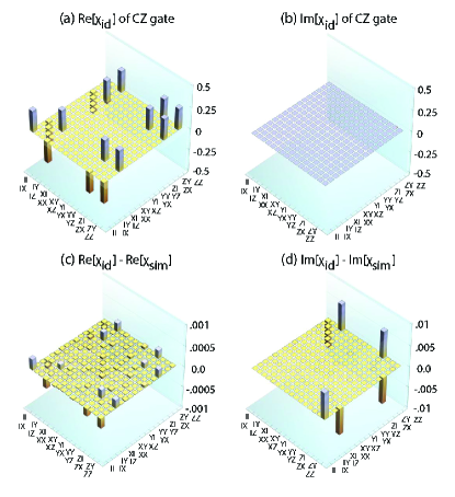
Figure 6: (color online) Ideal $\chi_{\rm id}$ matrix and the difference between ideal $\chi_{\rm id}$ and simulated $\chi_{\rm sim}$ matrices for QPT of the C_Z gate using the Jaksch, et al. pulse sequenceJaksch et al. (2000) for ⁸⁷Rb $112p_{1/2}$ states with $\Omega/2\pi=27.6~{}{\rm MHz}$. (a) Real part of $\chi_{\rm id}$, (b) Imaginary part of $\chi_{\rm id}$, (c) difference of real parts, ${\rm Re}[\chi_{\rm id}-\chi_{\rm sim}]$, and (d) difference of imaginary parts ${\rm Im}[\chi_{\rm id}-\chi_{\rm sim}]$.

Some insight can be gleaned into why the trace distance gives larger errors than the trace overlap as follows. The Jaksch et al. pulse sequence produces an imperfect $C_{Z}$ gate which can be written in the computational basis as

$$C_{Z} = \left(\begin{array}[]{cccc}1&0&0&0\\ 0&-1&0&0\\ 0&0&-1&0\\ 0&0&0&-e^{i\phi}\end{array}\right),$$ (22)

where $\phi=\pi\Omega/2{\sf B}$ is a small phase error in the strong blockade limit. As an example Fig. 6 shows the ideal $\chi$-matrix and the difference between the ideal and simulated $\chi$-matrices for the standard pulse sequence leading to (22). From Fig. 6(c) and (d), we can see that the error in the imaginary part of the $\chi$-matrix is much larger than that in the real part of the $\chi$-matrix. This is due to the fact that the real part is related to the amplitude errors for Rydberg blockade which are proportional to $\phi^{2}$, but the imaginary part is related to the phase error which scales as $\phi$.

Following the procedure for QPT in Ref. Nielsen and Chuang (2000) we can calculate the ideal and imperfect $\chi$-matrices from (22), and using Eqs. (17) we find the trace overlap and trace distance errors

$$E_{\rm O} = \frac{3}{8}\left[1-\cos(\phi)\right]\backsimeq\frac{3}{16}\phi^{2}\sim\left(\frac{\Omega}{\sf B}\right)^{2},$$ (23a)

$$E_{\rm D} = \frac{\sqrt{3}}{2}\sin(\phi/2)\backsimeq\frac{\sqrt{3}}{4}\phi\sim\frac{\Omega}{\sf B}.$$ (23b)

We see that $E_{\rm O}\sim\phi^{2}$ while $E_{\rm D}\sim\phi$ which verifies that the trace overlap is not sensitive to the imaginary part of $\chi$, which has linear phase errors, whereas the trace distance is sensitive to these errors.

Using the modified sequence of Fig. 3b we can correct the leading order linear term in the phase error. Doing so has negligible effect on the trace overlap since it is only sensitive to amplitude errors at ${\mathcal{O}}(\phi^{2})$. We do not report trace overlap errors for the modified pulse sequence in Table 3 since they are unchanged. However there is a large reduction in the trace distance error using the modified pulse sequence as can be seen from the values of $E_{\rm D}^{\prime}$ in the last row of the table. It has been common practice in experimental studies of quantum gate process fidelity to use the trace overlap as a reliable measure of the gate fidelity. The results shown in Table 3 highlight the fact that the trace overlap may give an overly optimistic view of the gate performance, since the trace distance gives larger errors. Identifying what type of errors are present and finding ways to minimize them, as we have done here using a modified pulse sequence, is facilitated by checking several error measures.

Finally we note that besides the intrinsic gate error sources, the dipole-dipole interaction will cause a momentum kick to both atoms Jaksch et al. (2000) which can excite a trap state without changing the internal state of the atoms when they are in Rydberg states. The perturbative transition probability is bounded by $p_{k}<(3\eta{\Omega}^{2}\Delta t/8{\sf B})^{2}/2$ with $\Delta t=2\pi/\Omega$ and $\eta=a/d\ll 1,$ where $a$ is the initial width of the atomic wave function determined by the trap and $d$ is the trap separation. For typical gate parameters and $\eta=1/50$ we find that $p_{k}<3\times 10^{-7}$ for Rb Rydberg $124p_{3/2}$ states which is much smaller than the QPT errors in Table 3. Thus errors due to momentum transfer between Rydberg excited atoms have a negligible effect on the gate fidelity.

V Discussion

An important motivation for performing detailed calculations of gate errors is to determine if Rydberg blockade could be used to build a fault tolerant, large scale quantum computing device. In order to answer that question it is necessary to make a connection between the fidelity measures, and the error limits for fault tolerant architectures that have been calculated theoretically. Threshold calculations typically proceed by assuming that an ideal unitary operator $U_{\rm id}$ describing the time evolution of the quantum circuit is corrupted by an error operator $U_{\rm er}$ with a small probability $\epsilon$, $0\leq\epsilon\leq 1$ so that the actual gate is described probabilistically as

$$U=(1-\epsilon)U_{\rm id}+\epsilon U_{\rm er}.$$

Depending on what assumptions are made about the types of error operators $U_{\rm er}$ that may occur, possible correlations between errors at different sites, and the overall system architecture, different threshold values $\epsilon_{\rm th}$ can be found. Provided $\epsilon<\epsilon_{\rm th}$ it is in principle feasible to build an arbitrarily large quantum processor. Calculations that make a minimum number of assumptions about $U_{\rm er}$ result in very low thresholds, $\epsilon_{\rm th}\sim 10^{-5}$Aliferis et al. (2006). Other calculations that make more restrictive assumptions result in higher thresholds. For example $\epsilon_{\rm th}>0.03$ in a model where the $U_{\rm er}$ are Pauli operatorsKnill (2005).

In order to relate the fidelity measures to thresholds for fault tolerance it is necessary to make explicit the connection between the process fidelity and the error probability $\epsilon$, as has been done for photonic quantum gatesWeinhold et al. (2008). We can estimate the lower bound on $\epsilon$ given a process fidelity as follows. Replace the process matrix in Eqs. (17) by $\chi_{\rm sim}\rightarrow(1-\epsilon)\chi_{\rm id}+\epsilon\chi_{\rm er}$ where $\chi_{\rm er}$ is the process matrix corresponding to the operator $U_{\rm er}$.

To derive lower bounds on $\epsilon$ we substitute the modified expression for $\chi_{\rm sim}$ into (17a) to get

$$E_{\rm O} = \epsilon{\rm Tr}^{2}\left[\sqrt{\sqrt{(\chi_{\rm id}-\chi_{\rm er})}\chi_{\rm id}\sqrt{(\chi_{\rm id}-\chi_{\rm er})}}\right]+O(\epsilon^{2}).$$

The right hand side is maximized for $\chi_{\rm er}=-\chi_{\rm id}$ and assuming small $\epsilon$ we find $E_{\rm O}\leq 2\epsilon.$ We can therefore use the trace overlap to bound the error probability from below according to

$$\epsilon_{\rm O}\geq\frac{E_{\rm O}}{2}.$$ (24)

Following the same steps for the trace distance gives

$$\epsilon_{\rm D}\geq E_{\rm D}.$$ (25)

These bounds result from assuming $\epsilon\ll 1$ and a worst case error process with ${\rm Tr}[\chi_{\rm id}\chi_{\rm er}]=-1$. Our calculated fidelity errors given in Table 3 are ${\mathcal{O}}(10^{-3})$ and we therefore have placed lower bounds on $\epsilon$ of ${\mathcal{O}}(10^{-3})$ which is below the threshold for some fault tolerant architectures.

Unfortunately this does not prove fault tolerance. We have bounded $\epsilon$ from below, but the actual $\epsilon$ for our gates may be higher. In addition, threshold calculations make assumptions about the types of errors that may occur, whereas our calculations of process fidelities are based on an independent physical model of the gate. In order to claim fault tolerance we would have to verify that the errors occurring in our simulations are compatible with the assumptions made in the threshold calculations. This has only been attempted for linear optics quantum gatesWeinhold et al. (2008) and is beyond the scope of the present paper. All we can say based on the results obtained here is that it is plausible that the fidelity of Rydberg blockade gates is sufficient to meet the threshold for fault tolerance in an appropriate architecture, but this has not been explicitly demonstrated.

In conclusion we have performed a detailed analysis and numerical simulation of our recent demonstration of a Rydberg blockade mediated CNOT gate between two individually addressed neutral atoms. Good agreement between the model and experimental results allows us to identify the leading error sources limiting the CNOT truth table fidelity as imperfect state preparation, spontaneous emission from the intermediate state during two-photon Rydberg excitation and imperfect Rydberg excitation and blockade due to variations of the atomic position at finite temperature. The fidelity of entangled Bell states created so far with Rydberg blockade is predominantly limited by ground-Rydberg dephasing due to Doppler broadening and magnetic field noise.

We have also found intrinsic error limits for Rydberg states which are accessible by one or two photon excitation through dipole allowed transitions. We show that the gate error cannot be made arbitrarily small by addressing higher lying Rydberg levels due to off-resonant coupling to neighboring levels which reduces the blockade effect. We identified the optimum blockade strength in the presence of neighboring Rydberg levels and showed using simulated QPT that for both ⁸⁷Rb and Cs atoms states can be found with process errors below $0.002$, provided we use a modified pulse sequence to correct small phase errors. The phase error correction assumes that the atoms are in the motional ground state of the optical traps. Our identification of optimum parameters including coupling to neighboring Rydberg levels is only approximate and it may be possible to further reduce the gate error with a more extensive parameter search.

While we have focused on the Rydberg blockade mechanism, the direct-interaction Rydberg phase gateJaksch et al. (2000), which uses simultaneous excitation of both atoms to a Rydberg level, may also be a route to high fidelity operation. Recent analysis of this gate using optimal control theory has identified parameters for which the gate error approaches $10^{-3}$ although a rigorous process error was not calculatedMüller et al. (2011). We note that also the phase gate which operates with the ordering $\Omega\gg{\sf B}$ will be subject to a limit on how high $n$ can be due to off-resonant excitation of neighboring Rydberg levels, as illustrated for the blockade gate in Fig. 5.

Our error results assume operation in a room temperature environment. The lifetimes of the $p_{3/2}$ states increase by about a factor of four in a 4K He cryostatBeterov et al. (2009a); *Beterov2009b, which would result in a reduction of the gate error by a factor of $\sim 2.5$ to a level below $10^{-3}$. Even lower error levels could in principle be reached using circular Rydberg states that have orders of magnitude longer lifetimes, although there are serious technical challenges connected with high fidelity excitation and de-excitation of these states.

Appendix A CNOT truth table error estimates with multiple Rydberg levels

In this appendix we present analytical estimates for the CNOT truth table including off-resonant excitation of multiple Rydberg levels. These estimates were used to find parameters for the process tomography calculations in Sec. IV.

A.1 Rydberg $np_{3/2}$ states

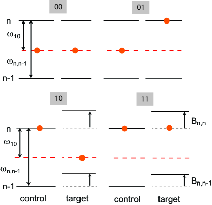
Figure 7: (color online) Off-resonant Rydberg excitation for $p$ states with $\omega_{n,n-1}>\omega_{10}$. The filled circles indicate the energies where the atoms are excited to with the long-dashed red lines corresponding to excitation of an atom starting in $|0\rangle$.

Alkali atom $np_{1/2}$ or $np_{3/2}$ levels can be reached by one-photon excitation from the ground state. The fine structure splitting of high $n$ Rydberg levels is relatively small, only 94 MHz for the Rb $100p$ states. This small splitting is problematic since resonant coupling to say $100p_{1/2}$ with a Rabi frequency of $\sim 10~{}\rm MHz$ would give errors at the $0.01$ level due to off-resonant coupling to $100p_{3/2}$. We therefore assume that the qubit state $|1\rangle$ is mapped onto the stretched ground state $f_{+}=I+1/2$, $m_{f}=f$ before and after Rydberg operations. When the stretched state is excited with $\sigma_{+}$ light angular momentum selection rules prevent coupling to $np_{1/2}$. We therefore only account for coupling to $np_{3/2},m_{j}=3/2$ states.

Referring to Fig. 7 we assume the spacing between neighboring levels $\omega_{n,n-1},$ satisfies $\omega_{n,n-1}>\omega_{10}$. This corresponds to Rydberg levels with $n\stackrel{{\scriptstyle<}}{{\sim}}100$ for the heavy alkalis. The leading contributions to blockade errors for the computational basis states are

$$E_{00} = \frac{3}{2}\left[\frac{\Omega^{2}}{\omega_{10}^{2}}+\frac{\Omega^{2}}{(\omega_{n,n-1}-\omega_{10})^{2}}\right]$$

$$E_{01} = \frac{2}{3}E_{00}$$

$$E_{10} = \frac{1}{2}\left[\frac{\Omega^{2}}{(\omega_{n,n-1}-{\sf B}_{n,n-1}-\omega_{10})^{2}}+\frac{\Omega^{2}}{(\omega_{10}+{\sf B}_{n,n})^{2}}\right]$$

$$E_{11} = \frac{1}{2}\left[\frac{\Omega^{2}}{{\sf B}_{n,n}^{2}}+\frac{\Omega^{2}}{(\omega_{n,n-1}-{\sf B}_{n,n-1})^{2}}\right].$$

The average blockade error is $E_{B}=\frac{1}{4}(E_{00}+E_{01}+E_{10}+E_{11}).$ We introduce two dimensionless parameters $a=\omega_{n,n-1}/\omega_{10}$ and $b={\sf B}_{n,n}/\omega_{10}.$ Parameter $a$ takes on discrete values as a function of Rydberg level $n$ while $b$ can be adjusted to minimize the error at fixed $n$ by changing the interatomic separation $d$. The blockade interaction between levels of different $n$ is also a function of $d$, but to a good approximation we can put ${\sf B}_{n,n-1}=b^{\prime}{\sf B}_{n,n}$, with $b^{\prime}$ a constant independent of $d$. We neglect contributions from coupling to level $n+1$ since the solutions found below have $b\sim 0.5$ and the average error from $n+1$ states only contributes at the 10% level.

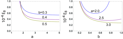
Figure 8: (color online) Blockade error scaling for $p$ states with $\omega_{n,n-1}>\omega_{10}$ as a function of $a,b$ with $\Omega/\omega_{10}=0.005$ and $b^{\prime}=1$.

The blockade error is minimized by ensuring that all undesired excitations are detuned as much as possible. This corresponds to $\omega_{n,n-1}$ very large but this is not a useful solution since it implies small $n$ and large spontaneous emission errors. In order to find a reasonable value for $n$ consider Fig. 8 which shows the blockade error for selected values of $a,b$. We see that for $a\sim 2.5$ and $b\sim 0.5$ the error is not far from the minimum possible. The scaled blockade shift $b$ could be made larger, but this would require very small values of the separation $d$ which implies difficulty in individual addressing of the atoms.

The above conditions are matched quite closely for ⁸⁷Rb (Cs) using $np_{3/2}$ states with $n=76(70).$ For ⁸⁷Rb with $n=76$ at $d=1.8~{}\mu\rm m$ we have $\omega_{76,75}=2\pi\times 17.0~{}\rm GHz$, $a=2.49$, $b=0.51$, $b^{\prime}=1.07$ which gives $E_{B}=0.63\times 10^{-4}$ at $\Omega/\omega_{10}=0.005$. For Cs with $n=70$ at $d=1.35~{}\mu\rm m$ we have $\omega_{70,69}=2\pi\times 23.0~{}\rm GHz$, $a=2.50$, $b=0.48$, $b^{\prime}=1.23$ which gives $E_{B}=0.66\times 10^{-4}$ at $\Omega/\omega_{10}=0.005$.

We can estimate the CNOT truth table error averaged over the computational basis states using the same procedure as in Sec. III. Including the spontaneous emission errors from Eq. (6), neglecting corrections of order $\Omega^{2}/\omega_{10}^{2},\Omega^{2}/{\sf B}^{2},$ the average error is

$$E=\frac{7\pi}{4\Omega\tau}+E_{B0}\Omega^{2}$$

where we have written $E_{B}=E_{B0}\Omega^{2}$. The optimum Rabi frequency is $\Omega_{\rm opt}=\left(\frac{7\pi}{8}\right)^{1/3}\frac{1}{(E_{B0}\tau)^{1/3}}$ which gives the minimum error for the computational basis states

$$E_{\rm cb}=\frac{3\left(7\pi\right)^{2/3}}{4}\frac{E_{B0}^{1/3}}{\tau^{2/3}}.$$ (26)

For ⁸⁷Rb $76p_{3/2}$ with $\tau=223~{}\mu\rm s$ we find $\Omega_{\rm opt}=2\pi\times 38.5~{}\rm MHz$ ($\Omega_{\rm opt}/\omega_{10}=0.006$) and $E_{\rm cb}=1.5\times 10^{-4}$. For Cs $70p_{3/2}$ with $\tau=211~{}\mu\rm s$ we find $\Omega_{\rm opt}=2\pi\times 47.1~{}\rm MHz$ ($\Omega_{\rm opt}/\omega_{10}=0.005$) and $E_{\rm cb}=1.3\times 10^{-4}$.

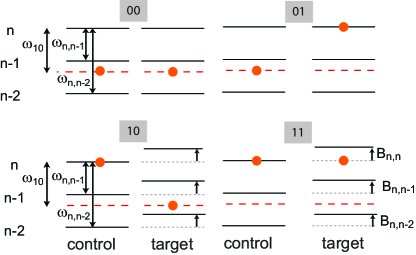
Figure 9: (color online) (color online) Off-resonant Rydberg excitation for $p$ states with $\omega_{n,n-1}>\omega_{10}>\omega_{n,n-2}$. The filled circles indicate the energies where the atoms are excited to with the long-dashed red lines corresponding to excitation of an atom starting in $|0\rangle$.

It is also possible to consider states with higher $n$ such that $\omega_{n,n-2}>\omega_{10}>\omega_{n,n-1}$. In this case, which is shown in Fig. 9, we must include off-resonant coupling to a third Rydberg level $n-2$. The effective blockade shift is now smaller than for the lower $n$ states but there is the advantage that the Rydberg lifetime is longer. The blockade errors for the computational basis states are

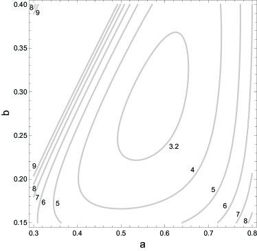
Figure 10: (color online) Blockade error scaling for $p$ states with $\omega_{n,n-2}>\omega_{10}>\omega_{n,n-1}$ as a function of $a,b$ with $\Omega/\omega_{10}=0.005$, $\omega_{n,n-2}=2\omega_{n,n-1}$, and $b^{\prime}=b^{\prime\prime}=1$ (${\sf B}_{n,n-2}=b^{\prime\prime}{\sf B}_{n,n}$). The contours are labeled with $E_{B}$ in units of $10^{-4}$.

$$E_{00} = \frac{3}{2}\left[\frac{\Omega^{2}}{(\omega_{10}-\omega_{n,n-1})^{2}}+\frac{\Omega^{2}}{(\omega_{n,n-2}-\omega_{10})^{2}}\right]$$

$$E_{01} = \frac{2}{3}E_{00}$$

$$E_{10} = \frac{1}{2}\left[\frac{\Omega^{2}}{(\omega_{10}-\omega_{n,n-1}+{\sf B}_{n,n-1})^{2}}\right.$$

$$\left.+\frac{\Omega^{2}}{(\omega_{n,n-2}-\omega_{10}-{\sf B}_{n,n-2})^{2}}\right]$$

$$E_{11} = \frac{1}{2}\left[\frac{\Omega^{2}}{{\sf B}_{n,n}^{2}}+\frac{\Omega^{2}}{(\omega_{n,n-1}-{\sf B}_{n,n-1})^{2}}\right].$$

The average blockade error $E_{B}=\frac{1}{4}(E_{00}+E_{01}+E_{10}+E_{11})$ is shown in Fig. 10.

The error is minimized for $a\sim 0.57$ and $b\sim 0.28$. These conditions are matched quite closely for ⁸⁷Rb (Cs) using $np_{3/2}$ states with $n=124(112).$ For ⁸⁷Rb with $n=124$ at $d=4.5~{}\mu\rm m$ we have $\omega_{124,123}=2\pi\times 3.73~{}\rm GHz$, $\omega_{124,122}=2\pi\times 7.55~{}\rm GHz$, $a=0.55$, $b=0.29$, $b^{\prime}=1.05$, $b^{\prime\prime}=1.06$ which gives $E_{B}=3.2\times 10^{-4}$ at $\Omega/\omega_{10}=0.005$. For Cs with $n=112$ at $d=3.2~{}\mu\rm m$ we have $\omega_{112,111}=2\pi\times 5.23~{}\rm GHz$, $\omega_{112,110}=2\pi\times 10.6~{}\rm GHz$, $a=0.57$, $b=0.29$, $b^{\prime}=1.19$, $b^{\prime\prime}=1.18$ which gives $E_{B}=3.4\times 10^{-4}$ at $\Omega/\omega_{10}=0.005$.

Using Eq. (26) we find the following CNOT truth table error estimates. For ⁸⁷Rb $124p_{3/2}$ with $\tau=616~{}\mu\rm s$ we find $\Omega_{\rm opt}=2\pi\times 16.3~{}\rm MHz$ ($\Omega_{\rm opt}/\omega_{10}=0.002$) and $E_{\rm cb}=1.3\times 10^{-4}$. For Cs $112p_{3/2}$ with $\tau=593~{}\mu\rm s$ we find $\Omega_{\rm opt}=2\pi\times 19.5~{}\rm MHz$ ($\Omega_{\rm opt}/\omega_{10}=0.002$) and $E_{\rm cb}=1.1\times 10^{-4}$.

We see that the truth table error estimates are slightly less than for the lower $n$ situation of Fig. 7. An additional advantage of using higher $n$ states is that the optimal blockade shift is reached with a larger $d\sim 3-4~{}\mu\rm m$ which may help to minimize qubit addressing crosstalk in an actual implementation. For convenience we have summarized all parameters for the states used in Table 4.

Table 4: Parameters of the Rydberg states used for QPT simulations. The scaling parameter $b^{\prime\prime}$ is defined as $b^{\prime\prime}={\sf B}_{n,n-2}/{\sf B}_{nn}$ for $np_{3/2},nd_{5/2}$ states and $b^{\prime\prime}={\sf B}_{n,n-1}^{\prime}/{\sf B}_{nn}$ for $ns_{1/2}$ states.

	87Rb				Cs
Rydberg state	$76p_{3/2}$	$124p_{3/2}$	$123d_{5/2}$	$82s_{1/2}$	$70p_{3/2}$	$112p_{3/2}$	$112d_{5/2}$	$80s_{1/2}$
$\omega_{10}/2\pi$ (GHz)	6.8	6.8	6.8	6.8	9.2	9.2	9.2	9.2
$\omega_{n,n-1}/2\pi$ (GHz)	17.0	3.7	3.7	13.7	23.0	5.2	5.1	15.3
$\omega_{n,n-2}/2\pi$ (GHz)		7.5	7.5			10.6	10.3
$\omega_{n,n-1}^{\prime}/2\pi$ (GHz)				-10.4				-8.5
$\omega_{n,n-2}^{\prime}/2\pi$ (GHz)				2.9				6.5
$\tau~{}(\mu\rm s)$	223	616	524	212	211	593	367	191
$d~{}(\mu\rm m)$	1.8	4.5	5.0	2.5	1.4	3.2	3.1	2.2
${\sf B}_{nn}/2\pi~{}\rm(GHz)$	3.45	2.0	1.9	3.3	4.4	2.6	2.5	3.9
$a=\omega_{n,n-1}/\omega_{10}$	2.5	0.55	0.54	2.0	2.5	0.57	0.55	1.7
$a^{\prime}=\omega_{n,n-1}^{\prime}/\omega_{10}$				-1.5				-0.93
$a^{\prime\prime}=\omega_{n,n-2}^{\prime}/\omega_{10}$				0.43				0.70
$b={\sf B}_{nn}/\omega_{10}$	0.51	0.29	0.27	0.48	0.48	0.29	0.27	0.43
$b^{\prime}={\sf B}_{n,n-1}/{\sf B}_{nn}$	1.1	1.0	0.77	0.95	1.2	1.2	0.98	0.75
$b^{\prime\prime}$		1.1	0.66	0.08		1.2	0.95	0.73
$b^{\prime\prime\prime}={\sf B}_{n,n-2}^{\prime}/{\sf B}_{nn}$				0.15				0.71

A.2 Rydberg $nd_{5/2}$ states

The issue of small fine structure splitting of the $p$ states discussed above, also applies to the $nd_{3/2},nd_{5/2}$ states. There are two ways of avoiding this problem. As with excitation of the $np$ states we may assume two-photon excitation from the stretched ground state with $\sigma_{+}$ light which only couples to $nd_{5/2},m_{j}=5/2$ states. Alternatively if the first leg of the excitation is made via the D1 transition ($5s_{1/2}-5p_{1/2}$ in Rb or $6s_{1/2}-6p_{1/2}$ in Cs) then only the $nd_{3/2},m_{j}=3/2$ states can be reached. Since we are setting the separation $d$ to give the desired blockade strength the only difference in the gate error using $nd_{3/2}$ or $nd_{5/2}$ states is due to differences in the lifetime. The lifetimes differ by only a few percent Beterov et al. (2009a) and we will therefore simply consider $nd_{5/2}$ states. The choice of optimum states and error analysis then follows that in Sec. A.1. We have summarized the parameters for the states used in Table 4.

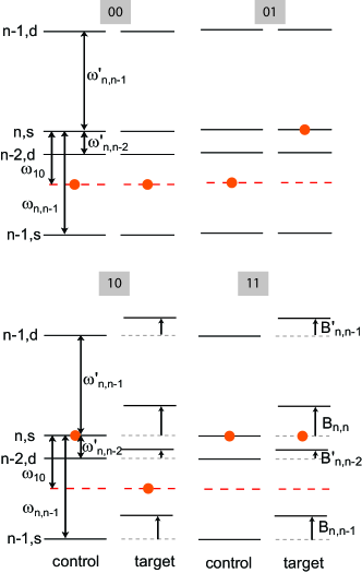
Figure 11: (color online) Off-resonant Rydberg excitation for $s$ states with $\omega_{n,n-1}>\omega_{10}$. Primed quantities refer to frequencies or blockade shifts between $s_{1/2}$ and $d_{3/2}$ states. The filled circles indicate the energies where the atoms are excited to with the long-dashed red lines corresponding to excitation of an atom starting in $|0\rangle$.

A.3 Rydberg $ns_{1/2}$ states

The $ns_{1/2}$ states have no fine-structure but there is an additional complication since it is not possible to use angular momentum selection rules to couple to $ns_{1/2}$ states, but not $nd_{3/2}$ or $nd_{5/2}$ states. We must therefore consider off-resonant coupling to additional Rydberg levels. The situation for $\omega_{n,n-1}>\omega_{10}$ is shown in Fig. 11. The leading contributions to blockade errors for the computational basis states are

$$E_{00} = \frac{3}{2}\left[\frac{\Omega^{2}}{\omega_{10}^{2}}+\frac{\Omega^{\prime 2}}{(\omega_{10}-\omega_{n,n-2}^{\prime})^{2}}+\frac{\Omega^{2}}{(\omega_{n,n-1}-\omega_{10})^{2}}\right]$$ (27a)

$$E_{01} = \frac{2}{3}E_{00}+\frac{\Omega^{\prime 2}}{2\omega_{n,n-2}^{\prime 2}}$$ (27b)

$$E_{10} = \frac{\Omega^{\prime 2}}{\omega_{n,n-2}^{\prime 2}}+\frac{\Omega^{2}}{2(\omega_{n,n-1}-{\sf B}_{n,n-1}-\omega_{10})^{2}}+\frac{\Omega^{\prime 2}}{2(\omega_{10}-\omega_{n,n-2}^{\prime}+{\sf B}_{n,n-2}^{\prime})^{2}}$$ (27c)

$$E_{11} = \frac{\Omega^{\prime 2}}{\omega_{n,n-2}^{\prime 2}}+\frac{\Omega^{2}}{2{\sf B}_{n,n}^{2}}+\frac{\Omega^{\prime 2}}{2(\omega_{n,n-2}^{\prime}-{\sf B}_{n,n-2}^{\prime})^{2}}.$$ (27d)

Here $\omega^{\prime},{\sf B}^{\prime}$ refer to frequencies and couplings between $s_{1/2}$ and $d_{3/2}$ states and $\Omega^{\prime}$ is the Rabi frequency for $nd_{3/2}$ excitation via the D1 transition from the ground state so that we need only consider $nd_{3/2}$ states. We introduce dimensionless parameters $a=\omega_{n,n-1}/\omega_{10}$, $a^{\prime}=\omega_{n,n-1}^{\prime}/\omega_{10}$, $a^{\prime\prime}=\omega_{n,n-2}^{\prime}/\omega_{10}$, $b={\sf B}_{n,n}/\omega_{10}$, $b^{\prime}={\sf B}_{n,n-1}/{\sf B}_{n,n}$, $b^{\prime\prime}={\sf B}_{n,n-1}^{\prime}/{\sf B}_{n,n}$, $b^{\prime\prime\prime}={\sf B}_{n,n-2}^{\prime}/{\sf B}_{n,n},$ and $c^{\prime}=\Omega^{\prime}/\Omega.$ Using $\sigma_{+},\sigma_{-}$ polarized excitation light for the ground-D1 and D1-Rydberg transitions $c^{\prime}=1.31$. Since $|\omega_{n,n-1}^{\prime}|\gg|\omega_{n,n-2}^{\prime}|$ we have neglected terms due to coupling to $n-1,d_{3/2}$ in (27). Additional checks with this level included give not more than 5% increase in the error averaged over the computational states. Since the computational cost of adding an additional Rydberg level in the master equation simulations is large we have neglected this small correction and performed master equation simulations with the three Rydberg states, $|r\rangle=|n,s_{1/2}\rangle,|r_{1}\rangle=|n-1,s_{1/2}\rangle,|r_{2}\rangle=|n-2,d_{3/2}\rangle$.

Numerical checks using Eqs. (27,26) were used to select the states listed in Table 4.