Gaussian processes for sample efficient reinforcement learning with RMAX-like exploration

Abstract

We present an implementation of model-based online reinforcement learning (RL) for continuous domains with deterministic transitions that is specifically designed to achieve low sample complexity. To achieve low sample complexity, since the environment is unknown, an agent must intelligently balance exploration and exploitation, and must be able to rapidly generalize from observations. While in the past a number of related sample efficient RL algorithms have been proposed, to allow theoretical analysis, mainly model-learners with weak generalization capabilities were considered. Here, we separate function approximation in the model learner (which does require samples) from the interpolation in the planner (which does not require samples). For model-learning we apply Gaussian processes regression (GP) which is able to automatically adjust itself to the complexity of the problem (via Bayesian hyperparameter selection) and, in practice, often able to learn a highly accurate model from very little data. In addition, a GP provides a natural way to determine the uncertainty of its predictions, which allows us to implement the “optimism in the face of uncertainty” principle used to efficiently control exploration. Our method is evaluated on four common benchmark domains.

1 Introduction

In reinforcement learning (RL), an agent interacts with an environment and attempts to choose its actions such that an externally defined performance measure, the accumulated per-step reward, is maximized over time. One defining characteristic of RL is that the environment is unknown and that the agent has to learn how to act directly from experience. In practical applications, e.g., in robotics, obtaining this experience means having a physical system interact with the physical environment in real time. Therefore, RL methods that are able to learn quickly and minimize the amount of time the robot needs to interact with the environment until good or optimal behavior is learned, are highly desirable.

In this paper we are interested in online RL for tasks with continuous state spaces and smooth transition dynamics that are typical for robotic control domains. Our primary goal is to have an algorithm which keeps sample complexity as low as possible.

1.1 Overview of the contribution

To maximize sample efficiency, we consider online RL that is model-based in the spirit of RMAX [3], but extended to continuous state spaces similar to [1, 10, 5]. As in RMAX and related methods, our algorithm, GP-RMAX, consists of two parts: a model-learner and a planner. The model-learner estimates the dynamics of the environment from the sample transitions the agent experiences while interacting with the environment. The planner is used to find the best possible action, given the current model. As the predictions of the model-learner become increasingly more accurate, the actions derived become increasingly closer to optimal. To control the amount of exploration, the “optimism in the face of uncertainty” principle is employed which makes the agent visit unexplored states first. In our algorithm, the model-learner is implemented by Gaussian process (GP) regression; being non-parametric, GPs give us enhanced modeling flexibility. GPs allow Bayesian model selection and automatic relevance determination. In addition, GPs provide a natural way to determine the uncertainty of predictions, which allows us to implement the “optimism in the face of uncertainty” exploration of RMAX in a principled way. The planner uses the estimated transition function (as estimated by the model) to solve the Bellman equation via value iteration on a uniform grid.

The key point of our algorithm is that we separate the steps estimating a function from samples in the model-learner from solving the Bellman equation in the planner. The rationale behind this is that, if the transition function is relatively simple, it can be estimated accurately from only few sample transitions. On the other hand, the optimal value function, due to the inclusion of the max operator, often is a complex function with sharp discontinuities. Solving the Bellman equation, however, does not require actual “samples”; instead, we must only be able to evaluate the Bellman operator in arbitrary points of the state space. This way, when the transition function can be learned from only a few samples, large gains in sample efficiency are possible. Competing model-free methods, such as fitted Q-iteration [18, 8, 15] or policy iteration based LSPI/LSTD/LSPE [12, 4, 13, 11], do not have this advantage, as they need the actual sample transitions to estimate and represent the value function.

Conceptually, our approach is closely related to Fitted R-MAX, which was proposed in [10] and uses an instance-based approach in the model-learner, and related work in [5, 1], which uses grid-based interpolation in the model-learner. The primary contribution of this paper is to use GPs instead. Doing this means we are willing to trade off theoretical analysis with practical performance. For example, unlike the recent ARL [1], for which PAC-style performance bounds could be derived (because of its grid-based implementation of model-learning), a GP is much better able to handle generalization and as a consequence can achieve much lower sample complexity.

1.2 Assumptions and limitations

Our approach makes the following assumptions (most of which are also made in related work, even if it is not always explicitly stated):

• Low dimensionality of the state space. With a uniform grid, the number of grid points for solving the Bellman equation scales exponentially with the dimensionality. While more advanced methods, such as sparse grids or adaptive grids, may allow us to somewhat reduce this exponential increase, at the end they do not break the curse of dimensionality. Alternatively, one can use nonlinear function approximation; however, despite some encouraging results, it is unclear as to whether this approach would really do any better in general applications. Today, breaking the curse of dimensionality is still an open research problem.

• Discrete actions. While continuous actions may be discretized, in practice, for higher dimensional action spaces this becomes infeasible.

• Smooth transition function. Performing an action from states that are “close” must lead to successor states that are “close”. (Otherwise both the generalization in the model learner and the interpolation in the value function approximation would not work).

• Deterministic transitions. This is not a fundamental requirement of our approach, since GPs can also learn noisy functions (either due to observation noise or random disturbances with small magnitude), and the Bellman operator can be evaluated in the resulting predictive distribution. Rather it is one taken for convenience.

• Known reward function. Assuming that the reward function is known and only the transition function needs to be learned is what is different from most comparable work. While it is not a fundamental requirement of our approach (since we could learn the reward function as well), it is an assumption that we think is well justified: for one, reward is the performance criterion and specifies the goal. For the type of control problems we consider here, reward is always externally defined and never something that is “generated” from within the environment. Two, reward sometimes is a discontinuous function, e.g., +1 at the goal state and 0 elsewhere. Which makes it not very amenable for function approximation.

2 Background: Planning when the model is exact

\psfrag{x00}{\scriptsize$\xi_{00}$}\psfrag{x10}{\scriptsize$\xi_{10}$}\psfrag{x11}{\scriptsize$\xi_{11}$}\psfrag{x01}{\scriptsize$\xi_{01}$}\psfrag{qza=}{\scriptsize$Q(z,a^{\prime})=?$}\psfrag{z=fxa}{\scriptsize$z:=f(\xi_{i},a)$}\psfrag{xi}{\scriptsize$\xi_{i}$}\psfrag{transitionf}{\scriptsize transition $f$}\psfrag{dx}{\scriptsize$d_{x}$}\psfrag{dy}{\scriptsize$d_{y}$}\psfrag{hx}{\scriptsize$h_{x}$}\psfrag{hy}{\scriptsize$h_{y}$}\psfrag{z=(xy)}{\scriptsize$z=(x,y)$}\psfrag{x0}{\scriptsize$x_{0}$}\psfrag{x1}{\scriptsize$x_{1}$}\includegraphics[width=112.73882pt]{grid1.eps}

\psfrag{x00}{\scriptsize$\xi_{00}$}\psfrag{x10}{\scriptsize$\xi_{10}$}\psfrag{x11}{\scriptsize$\xi_{11}$}\psfrag{x01}{\scriptsize$\xi_{01}$}\psfrag{qza=}{\scriptsize$Q(z,a^{\prime})=?$}\psfrag{z=fxa}{\scriptsize$z:=f(\xi_{i},a)$}\psfrag{xi}{\scriptsize$\xi_{i}$}\psfrag{transitionf}{\scriptsize transition $f$}\psfrag{dx}{\scriptsize$d_{x}$}\psfrag{dy}{\scriptsize$d_{y}$}\psfrag{hx}{\scriptsize$h_{x}$}\psfrag{hy}{\scriptsize$h_{y}$}\psfrag{z=(xy)}{\scriptsize$z=(x,y)$}\psfrag{x0}{\scriptsize$x_{0}$}\psfrag{x1}{\scriptsize$x_{1}$}\psfrag{x00}{\scriptsize$(\xi_{00},q_{00}^{a^{\prime}})$}\psfrag{x10}{\scriptsize$(\xi_{10},q_{10}^{a^{\prime}})$}\psfrag{x11}{\scriptsize$(\xi_{11},q_{11}^{a^{\prime}})$}\psfrag{x01}{\scriptsize$(\xi_{01},q_{01}^{a^{\prime}})$}\includegraphics[width=156.10345pt]{grid2.eps}

Figure 1: Bilinear interpolation to determine $Q(f(\xi_{i},a),a^{\prime})$ in $\mathbbm{R}^{2}$.

Consider the reinforcement learning problem for MDPs with continuous state space, finite action space, discounted reward criterion and deterministic dynamics [19]. In this section we assume that dynamics and rewards are available to the learning agent. Let state space $\mathcal{X}$ be a hyperrectangle in $\mathbbm{R}^{d}$ (this assumption is justified if, for example, the system is a motor control task), $\mathcal{A}$ be the finite action space (assuming continuous controls are discretized), $x_{t+1}=f(x_{t},a_{t})$ be the transition function (assuming that continuous time problems are discretized in time), and $r(x,a)$ be the reward function. For the following theoretical argument we require that both transition and reward function are Lipschitz continuous in the actions; i.e., there exist constants $L_{f},L_{r}$ such that $\left\|{f(x,a)-f(x^{\prime},a)}\right\|\leq L_{f}\left\|{x-x^{\prime}}\right\|$, and $|r(x,a)-r(x^{\prime},a)|\leq L_{r}\left\|{x-x^{\prime}}\right\|$, $\forall x,x^{\prime}\in\mathcal{X},a\in\mathcal{A}$. In addition, we assume that the reward is bounded, $|r(x,a)|\leq R_{\text{MAX}}$, $\forall x,a$. Note that in practice, while the first condition, continuity in the transition function, is usually fulfilled for domains derived from physical systems, the second condition, continuity in the rewards, is often violated (e.g. in the mountain car domain, reward is $0$ in the goal and $-1$ everywhere else). Despite that we find that in many of these cases the outlined procedure may still work well enough.

For any state $x$, we are interested in determining a sequence of actions $a_{0},a_{1},a_{2},\ldots$ such that the accumulated reward is maximized,

$$V^{*}(x):=\max_{a_{0},a_{1},\ldots}\ \Bigl{\{}\sum_{t=0}^{\infty}\gamma^{t}r(x_{t},a_{t})\ |\ x_{0}=x,x_{t+1}=f(x_{t},a_{t})\Bigr{\}},$$

where $0<\gamma<1$. Using the Q-notation, where $Q^{*}(x,a):=r(x,a)+\gamma V^{*}(f(x,a))$, the optimal decision policy $\pi^{*}$ is found by first solving the Bellman equation in the unknown function $Q$,

$$Q(x,a)=r(x,a)+\gamma\max_{a^{\prime}}\,Q(f(x,a),a^{\prime})\qquad\forall x\in\mathcal{X},a\in\mathcal{A}$$ (1)

to yield $Q^{*}$, and then choosing the action with the highest Q-value,

$$\pi^{*}(x)=\mathop{\mathrm{argmax}}_{a^{\prime}}\,Q^{*}(x,a^{\prime}).$$

The Bellman operator $T$ related to (1) is defined by

$$\bigl{(}TQ\bigr{)}(x,a):=r(x,a)+\gamma\max_{a^{\prime}}\,Q(f(x,a),a^{\prime}).$$ (2)

It is well known that $T$ is a contraction and $Q^{*}$ the unique bounded solution to the fixed point problem $Q(x,a)=\bigl{(}TQ\bigr{)}(x,a)$, $\forall x,a$.

In order to solve the infinite dimensional problem in (1) numerically, we have to reduce it to a finite dimensional problem. This is done by introducing a discretization $\Gamma$ of $\mathcal{X}$ into a finite number of elements, applying the Bellman operator to only the nodes and interpolating in between.

In the following we will consider a uniform grid $\Gamma_{h}$ with $N$ vertices $\xi_{i}$ and $d$-dimensional tensor B-spline interpolation of order $1$. The solution of (1) is then obtained in the space of piecewise affine functions.

For a fixed action $a^{\prime}$, the value $Q^{\Gamma_{h}}(z,a^{\prime})$ of any state $z$ with respect to grid $\Gamma_{h}$ can be written as a convex combination of the vertices $\xi_{j}$ of the grid cell enclosing $z$ with coefficients $w_{ij}$ (see Figure 1a). For example, consider the $2$-dimensional case (bilinear interpolation) in Figure 1b. Let $z=(x,y)\in\mathbbm{R}^{2}$. To determine $Q^{\Gamma_{h}}(z,a^{\prime})$, we find the four vertices $\xi_{00},\xi_{01},\xi_{10},\xi_{11}\in\mathbbm{R}^{2}$ of the enclosing cell with known function values $q_{00}^{a^{\prime}}:=Q^{\Gamma_{h}}(\xi_{00},a^{\prime}),\ldots$ etc. We then perform two linear interpolations along the $x$-coordinate (order invariant) in the auxilary points $x_{0},x_{1}$ to obtain

$$Q^{\Gamma_{h}}(x_{0},a^{\prime}) = (1-\lambda_{0})q_{00}^{a^{\prime}}+\lambda_{0}q_{01}^{a^{\prime}}$$

$$Q^{\Gamma_{h}}(x_{1},a^{\prime}) = (1-\lambda_{0})q_{10}^{a^{\prime}}+\lambda_{0}q_{11}^{a^{\prime}}$$

where $\lambda_{0}:=d_{x}/h_{x}$ (see Figure 1b for a definition of $d_{x},h_{x},x_{0},x_{1}$). We then perform another linear interpolation in $x_{0},x_{1}$ along the $y$-coordinate to obtain

$$Q^{\Gamma_{h}}(z,a^{\prime})=(1-\lambda_{1})(1-\lambda_{0})q_{00}^{a^{\prime}}+(1-\lambda_{1})\lambda_{0}q_{01}^{a^{\prime}}+\lambda_{1}(1-\lambda_{0})q_{10}^{a^{\prime}}+\lambda_{1}\lambda_{0}q_{11}^{a^{\prime}}$$ (3)

where $\lambda_{1}:=d_{y}/h_{y}$. Weights $w_{ij}$ now correspond to the coefficients in (3). An analogous procedure applies to higher dimensions.

Let $Q^{a^{\prime}}$ be the $N\times 1$ vector with entries $[Q^{a^{\prime}}]_{i}=Q^{\Gamma_{h}}(\xi_{i},a^{\prime})$. Let $z_{1}^{a},\ldots,z_{N}^{a}\in\mathbb{R}^{d}$ denote the successor state we obtain when we apply the transition function $f$ to vertices $\xi_{i}$ using action $a$, i.e., $z_{i}^{a}:=f(\xi_{i},a)$. Let $[w_{i}^{a}]_{j}=w_{ij}^{a}$ denote the $1\times N$ vector of coefficients for $z_{i}^{a}$ from (3). The Q-value of $z_{i}^{a}$ for any action $a^{\prime}$ with respect to grid $\Gamma_{h}$ can thus be written as $Q^{\Gamma_{h}}(z_{i}^{a},a^{\prime})=\sum_{j=1}^{N}[w_{i}^{a}]_{j}[Q^{a^{\prime}}]_{j}$. Let $W^{a}$ with rows $[w_{i}^{a}]$ be the $N\times N$ matrix of all coefficients. (Note that this matrix is sparse: each row contains only $2^{d}$ nonzero entries).

Let $R^{a}$ be the $N\times 1$ vector of associated rewards, $[R^{a}]_{i}:=r(\xi_{i},a)$. Now we can use (2) to obtain a fixed point equation in the vertices of the grid $\Gamma_{h}$,

$$Q^{\Gamma_{h}}(\xi_{i},a)=\bigl{(}T^{\Gamma_{h}}Q^{\Gamma_{h}}\bigr{)}(\xi_{i},a)\quad i=1,\ldots,N,\ a=1,\ldots,|\mathcal{A}|,$$ (4)

where

$$\bigl{(}T^{\Gamma_{h}}Q^{\Gamma_{h}}\bigr{)}(\xi_{i},a):=r(\xi_{i},a)+\gamma\max_{a^{\prime}}\,Q^{\Gamma_{h}}(f(\xi_{i},a),a^{\prime}).$$

Slightly abusing the notation, we can write this more compactly in terms of matrices and vectors,

$$T^{\Gamma_{h}}Q^{\Gamma_{h}}:=R^{a}+\gamma\max_{a^{\prime}}\,\bigl{\{}W^{a}Q^{a^{\prime}}\bigr{\}}\quad\forall a.$$ (5)

The Q-function is now represented by $|\mathcal{A}|$ $N$-dimensional vectors $Q^{a^{\prime}}$, each containing the values for the vertices $\xi_{i}$. The discretized Bellman operator $T^{\Gamma_{h}}$ is a contraction in $\mathbbm{R}^{d}\times\mathcal{A}$ and therefore has a unique fixed point $Q^{*}\in\mathbbm{R}^{d}\times\mathcal{A}$. Let function $Q^{*,{\Gamma_{h}}}:(\mathbbm{R}^{d}\times\mathcal{A})\rightarrow\mathbbm{R}$ be the Q-function obtained by linear interpolation of vector $Q^{*}$ along states. The function $Q^{*,{\Gamma_{h}}}$ can now be used to determine (approximately) optimal control actions: for any state $x\in\mathcal{X}$, we simply determine

$$\pi^{*,{\Gamma_{h}}}(x)=\mathop{\mathrm{argmax}}_{a^{\prime}}\,Q^{*,{\Gamma_{h}}}(x,a^{\prime}).$$

In order to estimate how well function $Q^{*,{\Gamma_{h}}}$ approximates the true $Q^{*}$, a posteriori estimates can be defined that are based on local errors, i.e. the maximum of residual in each grid cell. The local error in a grid cell in turn depends on the granularity of the grid, $h$, and the modulus of continuity $L_{f},L_{g}$ (e.g., see [9, 14] for details).

3 Our algorithm: GP-RMAX

\psfrag{xtt}{\tiny$x_{t+1}=f(x_{t},a_{t})$}\psfrag{xt}{\tiny$x_{t}$}\psfrag{at}{\tiny$a_{t}$}\psfrag{triplet}{\tiny$(x_{t},a_{t},x_{t+1})$}\psfrag{ftilde}{\tiny$\tilde{f}(x,a),c(x,a)$}\includegraphics[width=216.81pt]{modellearning_architecture_paths.eps}

Figure 2: High-level overview of the GP-RMAX framework

In the last section we have seen how, for a continuous state space, optimal behavior of an agent can be obtained in a numerically robust way, given that the transition function $x_{t+1}=f(x_{t},a_{t})$ is known.

For model-based RL we are now interested in solving the same problem for the case that the transition function is not known. Instead, the agent has to interact with the environment, and only use the samples it observes to compute optimal behavior. Our goal in this paper is to develop a learning framework where this number is kept as small as possible. This will be done by using the samples to learn an estimate $\tilde{f}(x,a)$ of $f(x,a)$ and then use this estimate $\tilde{f}$ in place of $f$ in the numerical procedure outlined in the previous section.

3.1 Overview

A sketch of our architecture is shown in Figure 2. GP-RMAX consists of the two parts model learning and planning which are interwoven for online learning. The model-learner estimates the dynamics of the environment from the sample transitions the agent experiences while interacting with the environment. The planner is used to find the best possible action, given the current model. As the predictions of the model-learner become increasingly more accurate, the actions derived from the planner become increasingly closer to optimal. Below is a high-level overview of the algorithm:

• Input:

  • Reward function $r(x,a)$

  • Discount factor $\gamma$

  • Performance parameters:

    • planning and model-update frequency $K$

    • model accuracy $\delta^{M}_{1},\delta^{M}_{2}$ (stopping criterion for model-learning)

    • discretization of planner $N$

• Initialize:

  • Model $\mathcal{M}_{1}$, Q-function $\mathcal{Q}_{1}$, observed transitions $\mathcal{D}_{1}$

• Loop: $t=1,2,\ldots$

  • Interact with system:

    • observe current state $x_{t}$

    • choose action $a_{t}$ greedy with respect to $\mathcal{Q}_{t}$

      $$a_{t}=\mathop{\mathrm{argmax}}_{a^{\prime}}\mathcal{Q}_{t}(x_{t},a^{\prime})$$

    • execute action $a_{t}$, observe next state $x_{t+1}$, store transition $\mathcal{D}_{t+1}=\mathcal{D}_{t}\cup\{x_{t},a_{t},x_{t+1}\}$

  • Model learning: (see Section 3.2)

    • only every $K$ steps, and only if $\mathcal{M}_{t}$ is not sufficiently exact (as determined by evaluating the stopping criterion)

      • $\mathcal{M}_{t+1}=\mathrm{update\_model}\,(\mathcal{M}_{t},\mathcal{D}_{t+1})$

      • $\mathrm{evaluate\_stopping\_criterion}\,(\mathcal{M}_{t+1},\mathcal{M}_{t},\delta^{M}_{1},\delta^{M}_{2})$

    • else

      • $\mathcal{M}_{t+1}=\mathcal{M}_{t}$

  • Planning with model: (see Section 3.3)

    • only every $K$ steps, and only if $\mathcal{M}_{t}$ is not sufficiently exact (as determined by evaluating the stopping criterion)

      • $\mathcal{Q}_{t+1}=\mathrm{augmented\_value\_iteration}\,(\mathcal{Q_{t}},\mathcal{M}_{t+1},@r(x,u),\gamma,N)$

    • else

      • $\mathcal{Q}_{t+1}=\mathcal{Q}_{t}$

Next, we will explain in more detail how each of the two functional modules “model-learner” and “planner” is implemented.

3.2 Model learning with GPs

In essence, estimating $\tilde{f}$ from samples is a regression problem. While in theory any nonlinear regression algorithm could serve this purpose, we believe that GPs are particularly well-suited: (1) being non-parametric means great modeling flexibility; (2) setting the hyperparameters can be done automatically (and in a principled way) via optimization of the marginal likelihood and allows automatic determination of relevant inputs; and (3) GPs provide a natural way to determine the uncertainty of its predictions which will be used to guide exploration. Furthermore, uncertainty in GPs is supervised in that it depends on the target function that is estimated (because of (2)); other methods only consider the density of the data (unsupervised) and will tend to overexplore if the target function is simple.

Assume we have observed a number of transitions, given as triplets of state, performed action, and resulting successor state, e.g., $\mathcal{D}=\{x_{t},a_{t},x_{t+1}\}_{t=1,2,\ldots}$ where $x_{t+1}=f(x_{t},a_{t})$. Note that $f$ is a $d$-dimensional function, $f(x_{t},a_{t})=\bigl{[}f_{1}(x_{t},a_{t}),\ldots,f_{d}(x_{t},a_{t})\bigr{]}^{T}$. Instead of trying to estimate $f$ directly (which corresponds to absolute transitions), we try to estimate the relative change $x_{t+1}-x_{t}$ as in [10]. The effect of each action on each state variable will be treated independently: we train multiple univariate GPs and combine the individual predictions afterwards. Each individual $\mathcal{GP}_{ij}$ is trained in the respective subset of data in $\mathcal{D}$, e.g., $\mathcal{GP}_{ij}$ is trained on all $x_{t}$ as input, and $x_{t+1}^{(i)}-x_{t}^{(i)}$ as output, where $a_{t}=j$. Each individual $\mathcal{GP}_{ij}$ has its own set of hyperparameters obtained from optimizing the marginal likelihood.

The details of working with GPs can be found in [17]; using GPs to learn a model for RL was previously also studied in [6] (for offline RL and without uncertainty-guided exploration). One characteristic of GPs is that their functional form is given in terms of a parameterized covariance function. Here we use the squared exponential,

$$k(x,x^{\prime};v_{0},b,\vec{\theta})=v_{0}\exp\Bigl{\{}-0.5(x-x^{\prime})^{T}\Omega(x-x^{\prime})\Bigr{\}}+b,$$

where matrix $\Omega$ is either one of the following: (1) $\Omega=\theta I$ (uniform), (2) $\Omega=\mathop{\mathrm{diag}}(\theta_{1},\ldots,\theta_{d})$ (axis aligned ARD), (3) $\Omega=M_{k}M_{k}^{T}$ (factor analysis). Scalars $v_{0},b$ and the ($\Omega$-dependent number of) entries of $\vec{\theta}$ constitute the hyperparameters of the GP and are adapted from the training data (likelihood optimization). Note that variant (2) and (3) implement automatic relevance determination: relevant inputs or linear projections of inputs are automatically identified, whereby model complexity is reduced and generalization sped up.

Once trained, for any testpoint $x$, $\mathcal{GP}_{ij}$ provides a distribution over target values, $\mathcal{N}(\mu_{ij}(x),\sigma_{ij}^{2}(x))$, with mean $\mu_{ij}(x)$ and variance $\sigma_{ij}^{2}(x)$ (exact formulas for $\mu$ and $\sigma$ can be found in [17]). Each individual mean $\mu_{ij}$ predicts the change in the $i$-th coordinate of the state under the $j$-th action. Each individual variance $\sigma_{ij}^{2}$ can be interpreted as the associated uncertainty; it will be close to $0$ if $\mathcal{GP}_{ij}$ is certain, and close to $k(x,x)$ if it is uncertain (the value of $k(x,x)$ depends on the hyperparameters of $\mathcal{GP}_{ij}$). Stacking the individual predictions together, our model-learner produces in summary

$$\tilde{f}(x,a):=\begin{bmatrix}x^{(1)}\\ \vdots\\ x^{(d)}\end{bmatrix}+\begin{bmatrix}\mu_{1a}(x)\\ \vdots\\ \mu_{da}(x)\end{bmatrix},\qquad c(x,a):=\max_{i=1,\ldots,d}\,\big{(}\mathrm{normalize}_{ia}(\sigma^{2}_{ia})\bigr{)},$$ (6)

where $\tilde{f}(x,a)$ is the predicted successor state and $c(x,a)$ the associated uncertainty (taken as maximum over the normalized per-coordinate uncertainties, where normalization ensures that the values lie between $0$ and $1$).

3.3 Planning with a model

At any time $t$, the planner receives as input model $\mathcal{M}_{t}$. For any state $x$ and action $a$, model $\mathcal{M}_{t}$ can be evaluated to “produce” the transition $\tilde{f}(x,a)$ along with normalized scalar uncertainty $c(x,a)\in[0,1]$, where $0$ means maximally certain and $1$ maximally uncertain (see Section 3.2)

Let ${\Gamma_{h}}$ be the discretization of the state space $\mathcal{X}$ with nodes $\xi_{i}$, $i=1,\ldots,N$. We now solve the planning stage by plugging $\tilde{f}$ into the procedure described in Section 2. First, we compute $\tilde{z}_{i}^{a}=\tilde{f}(\xi_{i},a)$, $c(\xi_{i},a)$ from (6) and the associated interpolation coefficients $w_{ij}^{a}$ from (3) for each node $\xi_{i}$ and action $a$.

Let $C^{a}$ denote the $N\times 1$ vector corresponding to the uncertainties, $[C^{a}]_{i}=c(\xi_{i},a)$; and $R^{a}$ be the $N\times 1$ vector corresponding to the rewards, $[R^{a}]_{i}=r(\xi_{i},a)$. To solve the discretized Bellman equation in Eq. (4), we perform basic Jacobi iteration:

• Initialize $[Q_{0}^{a}]_{i}$, $i=1,\ldots,N$, $a=1,\ldots,|A|$

• Repeat for $k=0,1,2,\ldots$

  $$[Q_{k+1}^{a}]_{i}=[R^{a}]_{i}+\gamma\max_{a^{\prime}}\left\{\sum_{j=1}^{N}w_{ij}^{a}[Q_{k}^{a^{\prime}}]_{j}\right\}\quad\forall i,a$$ (7)

  until $|Q_{k+1}^{a}-Q_{k}^{a}|_{\infty}<tol$, $\forall a$, or a maximum number of iterations is reached.

To reduce the number of iterations necessary, we adapt Grüne’s increasing coordinate algorithm [9] to the case of Q-functions: instead of Eq. (7), we perform updates of the form

$$[Q_{k+1}^{a}]_{i}=[1-\gamma w_{ii}^{a}]^{-1}\left([R^{a}]_{i}+\gamma\max_{a^{\prime}}\left\{\sum_{j=1,j\neq i}^{N}w_{ij}^{a}[Q_{k}^{a^{\prime}}]_{j}\right\}\right).$$ (7’)

In [9] it was proved that Eq. (7’) converges to the same fixed point as Eq. (7), and it was empirically demonstrated that convergence can occur in significantly fewer iterations. The exact reduction is problem-dependent, savings will be greater for small $\gamma$ and large cells where self-transitions occur (i.e., $\xi_{i}$ is among the vertices of the cell enclosing $\tilde{z}_{i}^{a}$).

To implement the “optimism in the face of uncertainty” principle, that is, to make the agent explore regions of the state space where the model predictions are uncertain, we employ the heuristic modification of the Bellman operator which was suggested in [15] and shown to perform well. Instead of Eq. (7’), the update rule becomes

$$[Q_{k+1}^{a}]_{i}=(1-[C^{a}]_{i})[1-\gamma w_{ii}^{a}]^{-1}\left([R^{a}]_{i}+\gamma\max_{a^{\prime}}\left\{\sum_{j=1,j\neq i}^{N}w_{ij}^{a}[Q_{k}^{a^{\prime}}]_{j}\right\}\right)+\\ +[C^{a}]_{i}V_{\text{MAX}}$$ (8)

where $V_{\text{MAX}}:=R_{\text{MAX}}/(1-\gamma)$. Eq. (8) can be seen as a generalization of the binary uncertainty in the original RMAX paper to continuous uncertainty; whereas in RMAX a state was either “known” (sufficiently explored), in which case the unmodified update was used, or “unknown” (not sufficiently explored), in which case the value $V_{\text{MAX}}$ was assigned, here the shift from exploration to exploitation is more gradual.

Finally we can take advantage of the fact that the planning function will be called many times during the process of learning. Since the discretization ${\Gamma_{h}}$ is kept fixed, we can reuse the final Q-values obtained in one call to plan as initial values for the next call to plan. Since updates to the model often affect only states in some local neighborhood (in particular in later stages), the number of necessary iterations in each call to planning will be further reduced.

A summary of our model-based planning function is shown below.

• Input:

  • Model $\mathcal{M}_{t}$, initial $[Q_{0}^{a}]_{i}$, $i=1,\ldots,N$, $a=1,\ldots,|A|$

• Static inputs:

  • Grid ${\Gamma_{h}}$ with nodes $\xi_{1},\ldots,\xi_{N}$, discount factor $\gamma$, reward function $r(x,a)$ evaluated in nodes giving $[R^{a}]_{i}$

• Initialize:

  • Compute $\tilde{z}_{i}^{a}=\tilde{f}(\xi_{i},a)$ and $[C^{a}]_{i}$ from $\mathcal{M}_{t}$ (see Eq. (6))

  • Compute weights $w_{ij}^{a}$ for each $\tilde{z}_{i}^{a}$ (see Eq. (3))

• Loop:

  • Repeat update Eq. (8) until $|Q_{k+1}^{a}-Q_{k}^{a}|_{\infty}<tol$, $\forall a$, or the maximum number of iterations is reached.

4 Experiments

We now examine the online learning performance of GP-RMAX in various well-known RL benchmark domains.

4.1 Description of domains

In particular, we choose the following domains (where a large number of comparative results is available in the literature):

Mountain car:

In mountain car, the goal is to drive an underpowered car from the bottom of a valley to the top of one hill. The car is not powerful enough to climb the hill directly, instead it has to build up the necessary momentum by reversing throttle and going up the hill on the opposite side first. The problem is $2$-dimensional, state variable $x_{1}\in[-1.2,0.5]$ describes the position of the car, $x_{2}\in[-0.07,0.07]$ its velocity. Possible actions are $a\in\{-1,0,+1\}$. Learning is episodic: every step gives a reward of $-1$ until the top of the hill at $x_{1}\geq 0.5$ is reached. Our experimental setup (dynamics and domain specific constants) is the same as in [19], with the following exceptions: maximal episode length is $500$ steps, discount factor $\gamma=0.99$ and every episode starts with the agent being at the bottom of the valley with zero velocity, $x_{\text{start}}=(-\pi/6,0)$.

Inverted pendulum:

The next task is to swing up and stabilize a single-link inverted pendulum. As in mountain car, the motor does not provide enough torque to push the pendulum up in a single rotation. Instead, the pendulum needs to be swung back and forth to gather energy, before being pushed up and balanced. This creates a more difficult, nonlinear control problem. The state space is $2$-dimensional, $\theta\in[-\pi,\pi]$ being the angle, $\dot{\theta}\in[-10,10]$ the angular velocity. Control force is discretized to $a\in\{-5,-2.5,0,+2.5,+5\}$ and held constant for $0.2$sec. Reward is defined as $r(x,a):=-0.1x_{1}^{2}-0.01x_{2}^{2}-0.01a^{2}$. The remaining experimental setup (equations of motion and domain specific constants) is the same as in [6]. The task is made episodic by resetting the system every $500$ steps to the initial state $x_{\text{start}}=(0,0)$. Discount factor $\gamma=0.99$.

Bicycle:

Next we consider the problem of balancing a bicycle that rides at a constant speed [8],[12]. The problem is $4$-dimensional: state variables are the roll angle $\omega\in[-12\pi/180,12\pi/180]$, roll rate $\dot{\omega}\in[-2\pi,2\pi]$, angle of the handle bar $\alpha\in[-80\pi/180,80\pi/180]$, and the angular velocity $\dot{\alpha}\in[-2\pi,2\pi]$. The action space is inherently $2$-dimensional (displacement of rider from the vertical and turning the handlebar); in RL it is usually discretized into $5$ actions. Our experimental setup so far is similar to [8]. To allow a more conclusive comparison of performance, instead of just being able to keep the bicycle from falling, we define a more discriminating reward $r(x,a)=-x_{1}^{2}$, and $r(x,a)=-10$ for $|x_{1}|<12\pi/180$ (bicycle has fallen). Learning is episodic: every episode starts in one of two (symmetric) states close to the boundary from where recovery is impossible: $x_{\text{start}}=(10\pi/180,0,0,0)$ or $x_{\text{start}}=(-10\pi/180,0,0,0)$, and proceeds for $500$ steps or until the bicycle has fallen. Discount factor $\gamma=0.98$.

Acrobot:

Our final problem is the acrobot swing-up task [19]. The goal is to swing up the tip of the lower link of an underactuated two-link robot over a given height (length of first link). Since only the lower link is actuated, this is a rather challenging problem. The state space is $4$-dimensional: $\theta_{1}\in[-\pi,\pi]$, $\dot{\theta}_{1}\in[-4\pi,4\pi]$, $\theta_{2}\in[-\pi,\pi]$, $\dot{\theta}_{2}\in[-9\pi,9\pi]$. Possible actions are $a\in\{-1,+1\}$. Our experimental setup and implementation of state transition dynamics is similar to [19]. The objective of learning is to reach a goal state as quickly as possible, thus $r(x,a)=-1$ for every step. The initial state for every episode is $x_{\text{start}}=(0,0,0,0)$. An episode ends if either a goal state is reached or $500$ steps have passed. The discount factor was set to $\gamma=1$, as in [19].

4.2 Results

We now apply our algorithm GP-RMAX to each of the four problems. The granularity of the discretization ${\Gamma_{h}}$ in the planner is chosen such that for the $2$-dimensional problems, the loss in performance due to discretization is negligible. For the $4$-dimensional problems, we ran offline trials with the true transition function to find the best compromise of granularity and computational efficiency. As result, we use a $100\times 100$ grid for mountain car and inverted pendulum, a $20\times 20\times 20\times 20$ grid for the bicycle balancing task, and a $25\times 25\times 25\times 25$ grid for the acrobot. The maximum number of value iterations was set to $500$, tolerance was $<10^{-2}$. In practice, running the full planning step took between 0.1-10 seconds for the small problems, and less than 5 min for the large problems (where often more than 50% of the CPU time was spent on computing the GP predictions in all the nodes of the grid). Using the planning module offline with the true transition function, we computed the best possible performance for each domain in advance. We obtained: mountain car (103 steps), inverted pendulum (-18.41 total cost), bicycle balancing (-3.49 total cost), and acrobot (64 steps).

For the GP-based model-learner, we set the maximum size of the subset to $1000$, and ICD tolerance to $10^{-2}$. The hyperparameters of the covariance were not manually tuned, but found from the data by likelihood optimiziation.

Since it would be computationally too expensive to update the model and perform the full planning step after every single observation, we set the planning frequency $K$ to $50$ steps. To gauge if optimal behavior is reached and further learning becomes unnessecary, we monitor the change in the model predictions and uncertainties between successive updates and stop if both fall below a threshold (test points in a fixed coarse grid).

We consider the following variations of the base algorithm: (1) GP-RMAXexp, which actively explores by adjusting the Bellman updates in Eq. (8) according to the uncertainties produced by the GP prediction; (2) GP-RMAXgrid, which does the same but uses binary uncertainty by overlaying a uniform grid on top of the state-action space and keeping track which cells are visited; and (3) GP-RMAXnoexp, which does not actively explore (see Eq. (7’)). For comparison, we repeat the experiments using the standard online model-free RL algorithm Sarsa($\lambda$) with tile coding [19], where we consider two different setup of the tilings (one finer and one coarser).

Figure 3 shows the result of online learning with GP-RMAX and Sarsa. In short, the graphs show us two things in particular: (1) GP-RMAX learns very quickly; and (2) GP-RMAX learns a behavior that is very close to optimal. In comparison, Sarsa($\lambda$) has a much higher sample complexity and does not always learn the optimal behavior (exception is the acrobot). While direct comparison with other high performance RL algorithms, such as fitted value iteration [18, 8, 15], policy iteration based LSPI/LSTD/LSPE [12, 4, 13, 11], or other kernel-based methods [7, 6] is difficult, because they are either batch methods or handle exploration in a more ad-hoc way, from the respective results given in the literature it is clear that for the domains we examined GP-RMAX performs relatively well.

Examining the plots in more detail, we find that, while GP-RMAXgrid is somewhat less sample efficient (explores more), GP-RMAXexp and GP-RMAXnoexp perform nearly the same. Initially, this appears to be in contrast with the whole point of RMAX, which is efficient exploration guided by the uncertainty of the predictions. Here, we believe that this behavior can be explained by the good generalization capabilities of GPs. Figure 4 illustrates model learning and certainty propagation with GPs in the mountain car domain (predicting acceleration as function of state). The state of the model-learner is shown for two snapshots: after 40 transitions and after 120 transitions. The top row shows the value function that results from applying value iteration with the update modified for uncertainty, see Eq. (8). The bottom row shows the observed samples and the associated certainty of the predictions. As expected, certainty is high in regions where data was observed. However, due to the generalization of GPs and data-dependent hyperparameter selection, certainty is also high in unexplored regions; and in particular it is constant along the $y$-coordinate. To understand this, we have to look at the state transition function of the mountain car: acceleration of the car indeed only depends on the position, but not on velocity. This shows that certainty estimates of GPs are supervised and take the properties of the target function into account, whereas prior RMAX treatments of uncertainty are unsupervised and only consider the density of samples to decide if a state is “known”. For comparison, we also show what GP-RMAX with grid-based uncertainty would produce in the same situation.

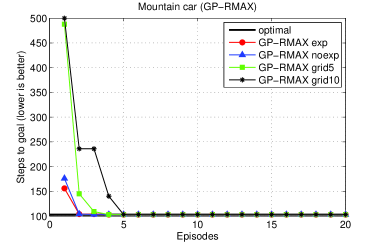
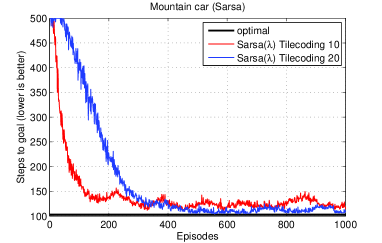
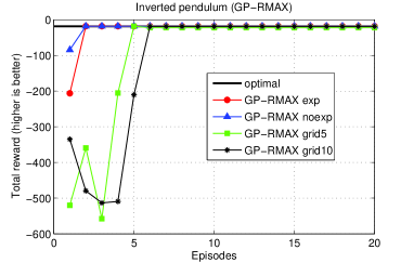
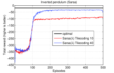
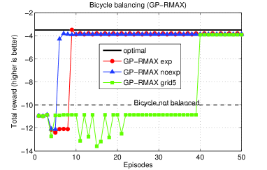
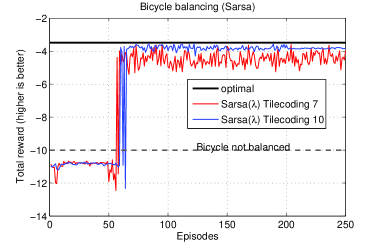
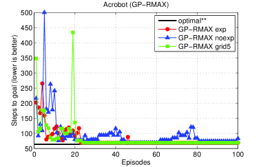
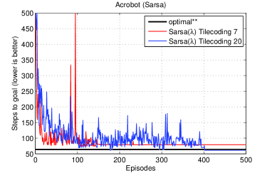
Figure 3: Learning curves of our algorithm GP-RMAX (left column) and the standard method Sarsa($\lambda$) with tile coding (right column) in the four benchmark domains. Each curve shows the online learning performance and plots the total reward as a function of the episode (and thus sample complexity). The black horizontal line denotes the best possible performance computed offline. Note the different scale of the x-axis between GP-RMAX and Sarsa.

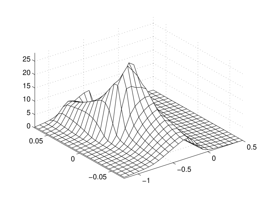
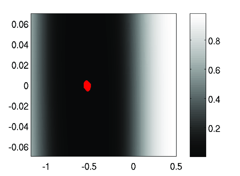
(a) GP after 40 samples

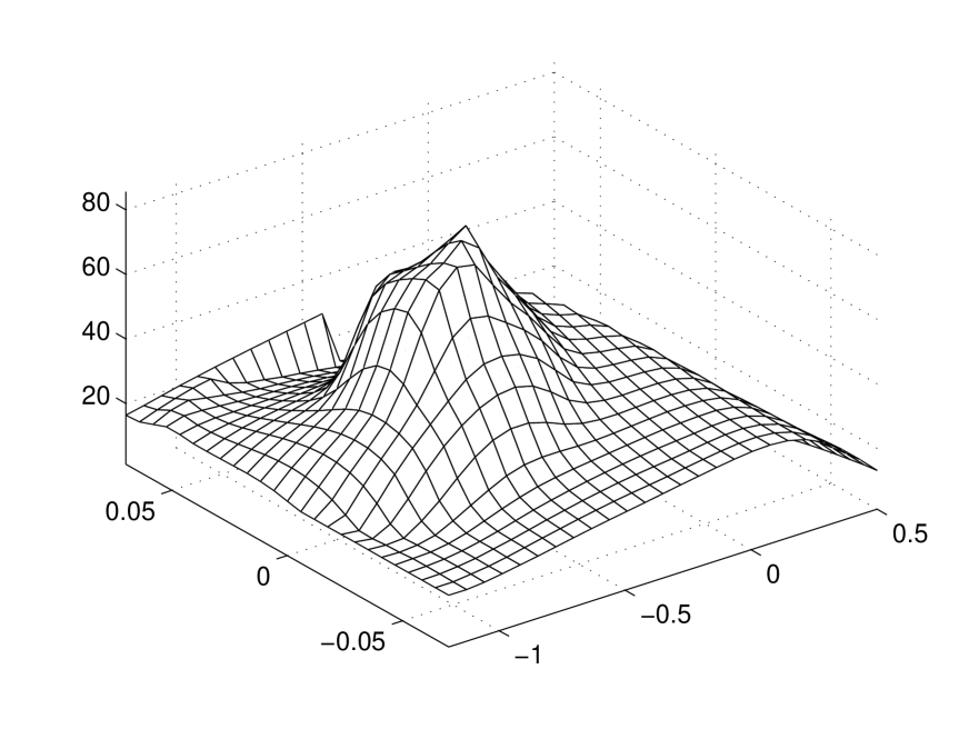
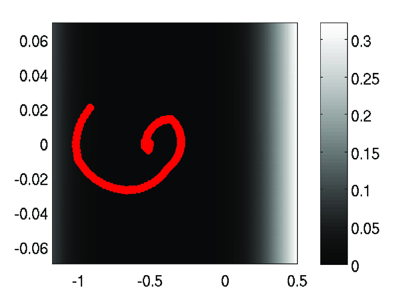
(b) GP after 120 samples

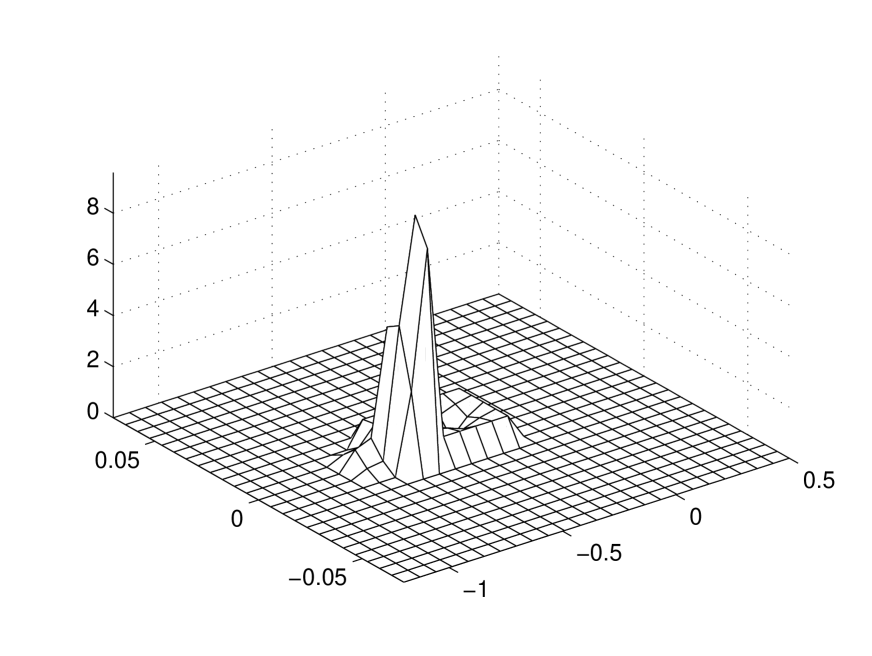
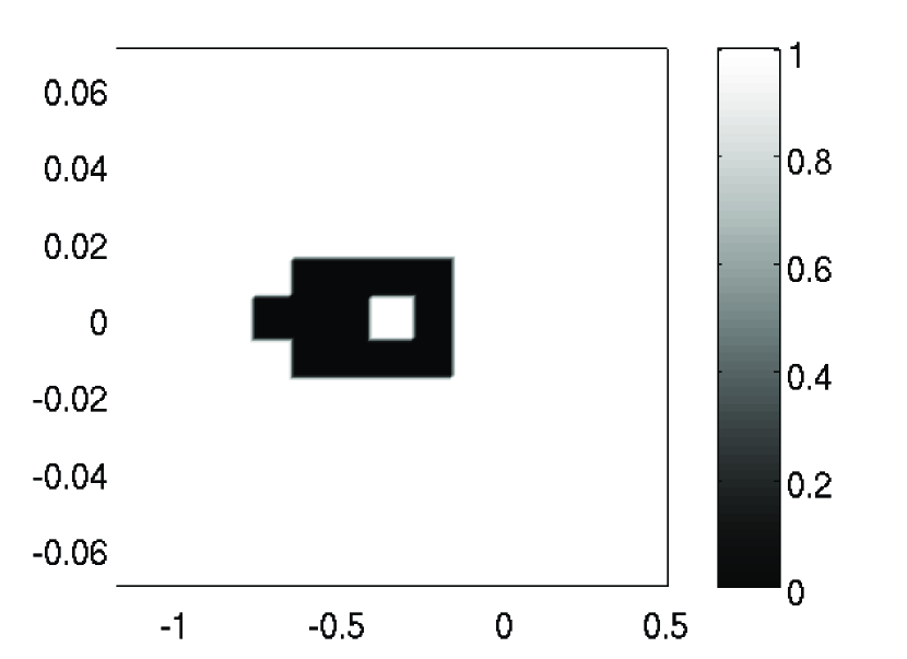
(c) Grid after 120 samples

Figure 4: Model-learning and propagation of “knownness” of state-action pairs with GPs. The top row shows the value function that results from applying value iteration with the update modified for uncertainty, see Eq. (8). The bottom row shows the actual samples (red circles) and the induced uncertainty of all states: black is perfectly “known”, white is perfectly “unknown”. Panels (a) and (b) show that with GPs certainty of model predictions is rapidly propagated through the whole state space, leading to strong generalization and targeted exploration. This in turn allows the optimal value function to be learned from very few sample transitions: panel (b) shows that after only 120 transitions (still in the middle of the very first episode) the approximated value function already resembles the true one [19]. Panel (c) shows the same for a counter-based binary uncertainty; most of the grid cells are unvisited and the thus the approximate value function is zero in most parts of the state space.

5 Summary

We presented an implementation of model-based online reinforcement learning similar to RMAX for continuous domains by combining GP-based model learning and value iteration on a grid. Doing so, our algorithm separates the problem function approximation in the model-learner from the problem function approximation/interpolation in the planner. If the transition function is easier to learn, i.e., requires only few samples relative to the representation of the optimal value function, then large savings in sample-complexity can be gained. Related model-free methods, such as fitted Q-iteration, can not take advantage of this situation. The fundamental limitation of our approach is that it relies on solving the Bellman equation globally over the state space. Even with more advanced discretization methods, such as adaptive grids, or sparse grids, the curse of dimensionality limits the applicability to problems with low or moderate dimensionality. Other, more minor limitations, concern the simplifying assumptions we made: deterministic state transitions and known reward function. However, these are not conceptual limitations but rather simplifying assumptions made for the present paper; they could be easily addressed in future work.

References

- [1] A. Bernstein and N. Shimkin. Adaptive-resolution reinforcement learning with efficient exploration. Machine Learning (published online: 5 May 2010). DOI:10.1007/s10994-010-5186-7, 2010.
- [2] G. Boone. Minimum-time control of the acrobot. Proc. of IEEE International Conference on Robotics and Automation, 4:3281–3287, 1997.
- [3] R. Brafman and M. Tennenholtz. R-MAX, a general polynomial time algorithm for near-optimal reinforcement learning. JMLR, 3:213–231, 2002.
- [4] L. Busoniu, D. Ernst, B. De Schutter, and R. Babuska. Online least-squares policy iteration for reinforcement learning control. In American Control Conference (ACC-10), 2010.
- [5] S. Davies. Multidimensional triangulation and interpolation for reinforcement learning. In NIPS 9. Morgan, 1996.
- [6] M. P. Deisenroth, C. E. Rasmussen, and J. Peters. Gaussian process dynamic programming. Neurocomputing, 72(7-9):1508–1524, 2009.
- [7] Y. Engel, S. Mannor, and R. Meir. Bayes meets Bellman: The Gaussian process approach to temporal difference learning. In Proc. of ICML 20, pages 154–161, 2003.
- [8] D. Ernst, P. Geurts, and L. Wehenkel. Tree-based batch mode reinforcement learning. JMLR, 6:503–556, 2005.
- [9] L. Grüne. An adaptive grid scheme for the discrete Hamilton-Jacobi-Bellman equation. Numerische Mathematik, 75:319–337, 1997.
- [10] N. K. Jong and P. Stone. Model-based exploration in continuous state spaces. In The 7th Symposium on Abstraction, Reformulation and Approximation, 2007.
- [11] T. Jung and D. Polani. Learning robocup-keepaway with kernels. JMLR: Workshop and Conference Proceedings (Gaussian Processes in Practice), 1:33–57, 2007.
- [12] M. G. Lagoudakis and R. Parr. Least-squares policy iteration. JMLR, 4:1107–1149, 2003.
- [13] L. Li, M. L. Littman, and C. R. Mansley. Online exploration in least-squares policy iteration. In Proc. of 8th AAMAS, 2009.
- [14] R. Munos and A. Moore. Variable resolution discretization in optimal control. Machine Learning, 49:291–323, 2002.
- [15] A. Nouri and M. L. Littman. Multi-resolution exploration in continuous spaces. In NIPS 21, 2008.
- [16] J. Quiñonero-Candela, C. E. Rasmussen, and C. K. I. Williams. Approximation methods for gaussian process regression. In Leon Bottou, Olivier Chapelle, Dennis DeCoste, and Jason Weston, editors, Large Scale Learning Machines, pages 203–223. MIT Press, 2007.
- [17] C. E. Rasmussen and C. K. I. Williams. Gaussian Processes for Machine Learning. MIT Press, 2006.
- [18] M. Riedmiller. Neural fitted q-iteration. In Proc. of 16th ECML, 2005.
- [19] R. Sutton and A. Barto. Reinforcement Learning: An Introduction. MIT Press, 1998.