Feature Selection for Value Function Approximation Using Bayesian Model Selection

Abstract

Feature selection in reinforcement learning (RL), i.e. choosing basis functions such that useful approximations of the unkown value function can be obtained, is one of the main challenges in scaling RL to real-world applications. Here we consider the Gaussian process based framework GPTD for approximate policy evaluation, and propose feature selection through marginal likelihood optimization of the associated hyperparameters. Our approach has two appealing benefits: (1) given just sample transitions, we can solve the policy evaluation problem fully automatically (without looking at the learning task, and, in theory, independent of the dimensionality of the state space), and (2) model selection allows us to consider more sophisticated kernels, which in turn enable us to identify relevant subspaces and eliminate irrelevant state variables such that we can achieve substantial computational savings and improved prediction performance.

1 Introduction

In this paper, we address the problem of approximating the value function under a stationary policy $\pi$ for a continuous state space $\mathcal{X}\subset\mathbbm{R}^{D}$,

$$V^{\pi}(\mathbf{x})=\mathbbm{E}_{\mathbf{x}^{\prime}|\mathbf{x},\pi(\mathbf{x})}\ \left\{R(\mathbf{x},\pi(\mathbf{x}),\mathbf{x}^{\prime})+\gamma V^{\pi}(\mathbf{x}^{\prime})\right\}$$ (1)

using a linear approximation of the form $\tilde{V}(\cdot\,;\mathbf{w})=\sum_{i=1}^{m}w_{i}\phi_{i}(\mathbf{x})$ to represent $V^{\pi}$. Here $\mathbf{x}$ denotes the state, $R$ the scalar reward and $\gamma$ the discount factor. Given a trajectory of states $\mathbf{x}_{1},\ldots,\mathbf{x}_{n}$ and rewards $r_{1},\ldots,r_{n-1}$ sampled under $\pi$, the goal is to determine weights $w_{i}$ (and basis functions $\phi_{i}$) such that $\tilde{V}$ is a good approximation of $V^{\pi}$. This is the fundamental problem arising in the policy iteration framework of infinite-horizon dynamic programming and reinforcement learning (RL), e.g. see [21, 3]. Unfortunately, this problem is also a very difficult problem that, at present, has no completely satisfying solution. In particular, deciding which features (basis functions $\phi_{i}$) to use is rather challenging, and in general, needs to be done manually: thus it is tedious, prone to errors, and most important of all, requires considerable insight into the domain. Hence, it would be far more desirable if a learning system could automatically choose its own representation. In particular, considering efficiency, we want to adapt to the actual difficulties faced, without wasting resources: often, there are many factors that can make a particular problem easier than it initially appears to be, for example, when only a few of the inputs are relevant, or when the input data lies on a low-dimensional submanifold of the input space.

Recent work in applying nonparametric function approximation to RL, such as Gaussian processes (GP) [6, 16, 18, 5], or equivalently, regularization networks [8], is a very promising step in this direction. Instead of having to explicitly specify individual basis functions, we only have to specify a more general kernel that just depends on a very small number of hyperparameters. The key contribution of this paper is to demonstrate that feature selection in RL from sample transitions can be automated, using any of several possible model selection methods for these hyperparameters, such as marginal likelihood optimization in a Bayesian setting, or leave-one-out (LOO) error minimization in a frequentist setting. Here, we will focus on the Bayesian setting, and adapt marginal likelihood optimization for the GP-based approximate policy evaluation method GPTD, introduced without model selection in [6]. Overall, this will have the following benefits: First, only by automatic model selection (as opposed to a grid-based search or manual tweaking of kernel parameters) will we be able to use more sophisticated kernels, which will allow us to uncover the ”hidden” properties of given problem. For example, by choosing an RBF kernel with independent lengthscales for the individual dimensions of the state space, model selection will automatically drive those components to zero that correspond to state variables irrelevant (or redundant) to the task. This will allow us to concentrate our computational efforts on the parts of the input space that really matter and will improve computational efficiency. Second, because it is generally easier to learn in ”smaller” spaces, it may also benefit generalization and thus help us to reduce sample complexity.

Despite its many promises, previous work with GPs in RL rarely explores the benefits of model selection: in [18], a variant of stochastic search was used to determine hyperparameters of the covariance for GPTD using as score function the online performance of an agent. In [16], standard GPs with marginal likelihood based model selection were employed; however, since their approach was based on fitted value iteration, the task of value function approximation was reduced to ordinary regression. The remaining paper is structured as follows: Section 2-3 contain background information and summarize the GPTD framework. As one of the benefits of model selection is the reduction of computational complexity, Section 4 describes how GPTD can be solved for large-scale problems using SR-approximation. Section 5 introduces model selection for GPTD and derives in detail the associated gradient computation. Finally, Section 6 illustrates our approach by providing experimental results.

2 Related work

The overall goal of learning representations and feature selection for linearly parameterized $\tilde{V}$ is not new within the context of RL. Roughly, past methods can be categorized along two dimensions: how the basis functions are represented (e.g. either by parameterized and predefined basis functions such as RBF, or by nonparameterized basis functions directly derived from the data) and what quantity/target function is considered to guide their construction process (e.g. either supervised methods that consider the Bellman error and depend on the particular reward/goal, or unsupervised graph-based methods that consider connectivity properties of the state space). Conceptually closely related to our work is the approach described in [12], which adapts the hyperparameters of RBF-basis functions (both their location and lengthscales) using either gradient descent or the cross-entropy method on the Bellman error. However, because basis functions are adapted individually (and their number is chosen in advance), the method is prone to overfitting: e.g. by placing basis functions with very small width near discontinuities. The problem is compounded when only few data points are available. In contrast, using a Bayesian approach, we can automatically trade-off model fit and model complexity with the number of data points, choosing always the best complexity: e.g. for small data sets we will prefer larger lengthscales (less complex), for larger data sets we can afford smaller lengthscales (more complex).

Other alternative approaches do not rely on predefined basis functions: The method in [9] is an incremental approach that uses dimensionality reduction and state aggregation to create new basis functions such that for every step the remaining Bellman error for a trajectory of states is successively reduced. A related approach is given in [14] which incrementally constructs an orthogonal basis for the Bellman error. A graph-based unsupervised approach is presented in [11], which derives basis functions from the eigenvectors of the graph Laplacian induced from the underlying MDP.

3 Background: GPs for policy evaluation

In this section we briefly summarize how GPs [17] can be used for approximate policy evaluation; here we will follow the GPTD formulation of [6].

Suppose we have observed the sequence of states $\mathbf{x}_{1},\mathbf{x}_{2},\ldots,\mathbf{x}_{n}$ and rewards $r_{1},\ldots,r_{n-1}$, where $\mathbf{x}_{i}\sim p(\cdot\,|\,\mathbf{x}_{i-1},\pi(\mathbf{x}_{i-1}))$ and $r_{i}=R(\mathbf{x}_{i},\pi(\mathbf{x}_{i}),\mathbf{x}_{i+1})$. In practice, MDPs considered in RL will often be of an episodic nature with absorbing terminal states. Therefore we have to transform the problem such that the resulting Markov chain is still ergodic: this is done by introducing a zero reward transition from the terminal state of one episode to the start state of the next episode. In addition to the sequence of states and rewards our training data thus also includes a sequence $\gamma_{1},\ldots,\gamma_{n-1}$, where $\gamma_{i}=\gamma$ (the discount factor in Eq. (1)) if $\mathbf{x}_{i+1}$ was a non-terminal state, and $\gamma_{i}=0$ if $\mathbf{x}_{i}$ was a terminal state (in which case $\mathbf{x}_{i+1}$ is the start state of the next episode).

Assume that the function values $V(\mathbf{x})$ of the unknown value function $V:\mathcal{X}\subset\mathbbm{R}^{D}\rightarrow R$ from Eq. (1) form a zero-mean Gaussian process with covariance function $k(\mathbf{x},\mathbf{x}^{\prime})$ for $\mathbf{x},\mathbf{x}^{\prime}\in\mathcal{X}$; in short $V\sim\mathcal{GP}(\boldsymbol{0},k(\mathbf{x},\mathbf{x}^{\prime}))$. In consequence, the function values for the $n$ observed states, $\mathbf{v}:=\bigl{(}V(\mathbf{x}_{1}),\ldots,V(\mathbf{x}_{n})\bigr{)}^{\text{T}}$, will have a Gaussian distribution

$$\mathbf{v}\,|\,\mathbf{X},\boldsymbol{\theta}\ \sim\ \mathcal{N}(\boldsymbol{0},\mathbf{K}),$$ (2)

where $\mathbf{X}:=[\mathbf{x}_{1},\ldots,\mathbf{x}_{n}]$ and $\mathbf{K}$ is the $n\times n$ covariance matrix with entries $[\mathbf{K}]_{ij}=k(\mathbf{x}_{i},\mathbf{x}_{j})$. Note that the covariance $k(\cdot,\cdot)$ alone fully specifies the GP; here we will assume that it is a simple (positive definite) function parameterized by a number of scalar parameters collected in vector $\boldsymbol{\theta}$ (see Section 4).

However, unlike in ordinary regression, in RL we cannot observe samples from the target function $V$ directly. Instead, the values can only be observed indirectly: from Eq. (1) we have that the value of one state is recursively defined through the value of the successor state(s) and the immediate reward. To this end, Engel et al. propose the following generative model:

$$R(\mathbf{x}_{i},\mathbf{x}_{i+1})=V(\mathbf{x}_{i})-\gamma_{i}V(\mathbf{x}_{i+1})+\eta_{i},$$ (3)

where $\eta_{i}$ is a noise term that may depend on the inputs. Plugging in the observed training data, and defining $\mathbf{r}:=\bigl{(}r_{1},\ldots,r_{n-1}\bigr{)}^{\text{T}}$, we obtain

$$\mathbf{r}=\mathbf{H}\mathbf{v}+\boldsymbol{\eta},$$ (4)

where the $(n-1)\times n$ matrix $\mathbf{H}$ is given by

$$\mathbf{H}:=\begin{bmatrix}1&-\gamma_{1}&&\\ &\ddots&\ddots&\\ &&1&-\gamma_{n-1}\end{bmatrix}$$ (5)

and noise $\boldsymbol{\eta}:=\bigl{(}\eta_{1},\ldots,\eta_{n-1}\bigr{)}^{\text{T}}$ has distribution $\boldsymbol{\eta}\sim\mathcal{N}(\boldsymbol{0},\boldsymbol{\Sigma})$. One first choice for the noise covariance $\boldsymbol{\Sigma}$ would be $\boldsymbol{\Sigma}=\sigma_{0}^{2}\mathbf{I}$, where $\sigma_{0}^{2}$ is an unknown hyperparameter (see Section 4). However, this model does not capture stochastic state transitions and hence would only be applicable for deterministic MDPs. If the environment is stochastic, the noise model $\boldsymbol{\Sigma}=\sigma_{0}^{2}\mathbf{H}\mathbf{H}^{\text{T}}$ is more appropriate, see [6] for more detailed explanations. For the remainder we will solely consider the latter choice, i.e. $\boldsymbol{\Sigma}=\sigma_{0}^{2}\mathbf{H}\mathbf{H}^{\text{T}}$.

Let $\mathcal{D}:=\{\mathbf{X},\gamma_{1},\ldots,\gamma_{n-1}\}$ be an abbreviation for the training inputs. Using Eq. (4), it can be shown that the joint distribution of the observed rewards $\mathbf{r}$ given inputs $\mathcal{D}$ is again a Gaussian,

$$\mathbf{r}\,|\,\mathcal{D},\boldsymbol{\theta}\ \sim\mathcal{N}(\boldsymbol{0},\mathbf{Q}),$$ (6)

where the $(n-1)\times(n-1)$ covariance matrix $\mathbf{Q}$ is given by

$$\mathbf{Q}=\bigl{(}\mathbf{H}\mathbf{K}\mathbf{H}^{\text{T}}+\sigma_{0}^{2}\mathbf{H}\mathbf{H}^{\text{T}}\bigr{)}.$$ (7)

To predict the function value $V(\mathbf{x}^{*})$ at a new state $\mathbf{x}^{*}$, we consider the joint distribution of $\mathbf{r}$ and $V(\mathbf{x}^{*})$

$$\begin{bmatrix}\mathbf{r}\\ V(\mathbf{x}^{*})\end{bmatrix}\,|\,\mathcal{D},\mathbf{x}^{*},\boldsymbol{\theta}\ \sim\ \mathcal{N}\left(\begin{bmatrix}\boldsymbol{0}\\ 0\end{bmatrix},\begin{bmatrix}\mathbf{Q}&\mathbf{H}\mathbf{k}(\mathbf{x}^{*})\\ [\mathbf{H}\mathbf{k}(\mathbf{x}^{*})]^{\text{T}}&k^{*}\end{bmatrix}\right)$$

where $n\times 1$ vector $\mathbf{k}(\mathbf{x}^{*})$ is given by $\mathbf{k}(\mathbf{x}^{*}):=\bigl{(}k(\mathbf{x}^{*},\mathbf{x}_{1}),\ldots,k(\mathbf{x}^{*},\mathbf{x}_{n})\bigr{)}^{\text{T}}$ and scalar $k^{*}$ by $k^{*}:=k(\mathbf{x}^{*},\mathbf{x}^{*})$. Conditioning on $\mathbf{r}$, we then obtain

$$V(\mathbf{x}^{*})\,|\,\mathcal{D},\mathbf{r},\mathbf{x}^{*},\boldsymbol{\theta}\ \sim\ \mathcal{N}(\boldsymbol{\mu}(\mathbf{x}^{*}),\sigma^{2}(\mathbf{x}^{*}))$$ (8)

where

$$\boldsymbol{\mu}(\mathbf{x}^{*}) :=\mathbf{k}(\mathbf{x}^{*})^{\text{T}}\mathbf{H}^{\text{T}}\mathbf{Q}^{-1}\mathbf{r}$$ (9)

$$\sigma^{2}(\mathbf{x}^{*}) :=k^{*}-\mathbf{k}(\mathbf{x}^{*})^{\text{T}}\mathbf{H}^{\text{T}}\mathbf{Q}^{-1}\mathbf{H}\mathbf{k}(\mathbf{x}^{*}).$$ (10)

Thus, for any given single state $\mathbf{x}^{*}$, GPTD produces the distribution $p(V(\mathbf{x}^{*})|\mathcal{D},\mathbf{r},\mathbf{x}^{*},\boldsymbol{\theta})$ in Eq. (8) over function values.

4 Computational considerations

Regarding its implementation, GPTD for policy evaluation shares the same weakness that GPs have in traditional machine learning tasks: solving Eq. (8) requires the inversion of a dense $(n-1)\times(n-1)$ matrix, which when done exactly would require $\mathcal{O}(n^{3})$ operations and is hence infeasible for anything but small-scale problems (say, anything with $n<5000$).

4.1 Subset of regressors

In the subset of regressors (SR) approach initially proposed for regularization networks [15, 10], one chooses a subset $\{\mathbf{\tilde{x}}\}_{i=1}^{m}$ of the data, with $m\ll n$, and approximates the covariance for arbitrary $\mathbf{x},\mathbf{x}^{\prime}$ by taking

$$\tilde{k}(\mathbf{x},\mathbf{x}^{\prime})=\mathbf{k}_{m}(\mathbf{x})^{\text{T}}\mathbf{K}_{mm}^{-1}\mathbf{k}_{m}(\mathbf{x}^{\prime}).$$ (11)

Here $\mathbf{k}_{m}(\cdot)$ denotes $\mathbf{k}_{m}(\cdot):=\bigl{(}k(\mathbf{\tilde{x}}_{1},\cdot),\ldots,k(\mathbf{\tilde{x}}_{m},\cdot)\bigr{)}^{\text{T}}$, and $\mathbf{K}_{mm}$ is the submatrix $[\mathbf{K}_{mm}]_{ij}=k(\mathbf{\tilde{x}}_{i},\mathbf{\tilde{x}}_{j})$ of $\mathbf{K}$. The approximation in Eq. (11) can be motivated for example from the Nyström approximation [22]. Let $\mathbf{K}_{nm}$ denote the submatrix $[\mathbf{K}_{nm}]_{ij}=k(\mathbf{x}_{i},\mathbf{\tilde{x}}_{j})$ corresponding to the $m$ columns of the data points in the subset. We then have the rank-reduced approximation $\mathbf{K}\approx\mathbf{\tilde{K}}=\mathbf{K}_{nm}\mathbf{K}_{mm}^{-1}\mathbf{K}_{nm}^{\text{T}}$ and $\mathbf{k}(\mathbf{x})\approx\mathbf{\tilde{k}}(\mathbf{x})=\mathbf{K}_{nm}\mathbf{K}_{mm}^{-1}\mathbf{k}_{m}(\mathbf{x})$. Plugging these into Eq. (8), we obtain for the mean

$$\boldsymbol{\mu}(\mathbf{x}^{*}) \approx\mathbf{\tilde{k}}(\mathbf{x}^{*})^{\text{T}}\mathbf{H}^{\text{T}}\bigl{(}\mathbf{H}\mathbf{\tilde{K}}\mathbf{H}^{\text{T}}+\sigma_{0}^{2}\mathbf{H}\mathbf{H}^{\text{T}}\bigr{)}^{-1}\mathbf{r}$$

$$=\mathbf{k}_{m}(\mathbf{x}^{*})^{\text{T}}\bigl{(}\mathbf{G}^{\text{T}}\mathbf{W}\mathbf{G}+\sigma_{0}^{2}\mathbf{K}_{mm}\bigr{)}^{-1}\mathbf{G}^{\text{T}}\mathbf{W}\mathbf{r},$$ (12)

where we have defined $\mathbf{G}:=\mathbf{H}\mathbf{K}_{nm}$, $\mathbf{W}:=(\mathbf{H}\mathbf{H}^{\text{T}})^{-1}$ and applied the SMW identity to show that

$$\mathbf{K}_{mm}^{-1}\mathbf{G}^{\text{T}}\bigl{(}\mathbf{G}\mathbf{K}_{mm}^{-1}\mathbf{G}^{\text{T}}+\sigma_{0}^{2}\mathbf{W}^{-1}\bigr{)}^{-1}=\bigl{(}\mathbf{G}^{\text{T}}\mathbf{W}\mathbf{G}+\sigma_{0}^{2}\mathbf{K}_{mm}\bigr{)}^{-1}\mathbf{G}^{\text{T}}\mathbf{W}.$$ (13)

Similarly, we obtain for the predictive variance

$$\sigma(\mathbf{x}^{*}) \approx\tilde{k}(\mathbf{x}^{*},\mathbf{x}^{*})-\mathbf{\tilde{k}}(\mathbf{x}^{*})^{\text{T}}\mathbf{H}^{\text{T}}\bigl{(}\mathbf{H}\mathbf{\tilde{K}}\mathbf{H}^{\text{T}}+\sigma_{0}^{2}\mathbf{H}\mathbf{H}^{\text{T}}\bigr{)}^{-1}\mathbf{H}\mathbf{\tilde{k}}(\mathbf{x}^{*})$$

$$=\sigma_{0}^{2}\mathbf{k}_{m}(\mathbf{x}^{*})^{\text{T}}\bigl{(}\mathbf{G}^{\text{T}}\mathbf{W}\mathbf{G}+\sigma_{0}^{2}\mathbf{K}_{mm}\bigr{)}^{-1}\mathbf{k}_{m}(\mathbf{x}^{*}).$$ (14)

Doing this means a huge gain in computational savings: solving the reduced problem in Eq. (12) costs $\mathcal{O}(m^{2}n)$ for initialization, requires $\mathcal{O}(m^{2})$ storage and every prediction costs $\mathcal{O}(m)$ (or $\mathcal{O}(m^{2})$ if we additionally evaluate the variance). This has to be compared with the complexity of the full problem: $\mathcal{O}(n^{3})$ initialization, $\mathcal{O}(n^{2})$ storage, and $\mathcal{O}(n)$ prediction. Thus computational complexity now only depends linearly on $n$ (for constant $m$).

Note that the SR-approximation produces a degenerate GP. As a consequence, the predictive variance in Eq. (14) will underestimate the true variance. In particular, it will be near zero when $\mathbf{x}$ is far from the subset $\{\mathbf{\tilde{x}}\}_{i=1}^{m}$ (which is exactly the opposite of what we want, as the predictive variance should be high for novel inputs). The situation can be remedied by considering the projected process approximation [4, 19], which results in the same expression for the mean in Eq. (12), but adds the term

$$k(\mathbf{x}^{*},\mathbf{x}^{*})-\mathbf{k}_{m}(\mathbf{x}^{*})^{\text{T}}\mathbf{K}_{mm}^{-1}\mathbf{k}_{m}(\mathbf{x}^{*})$$ (15)

to the variance in Eq. (14)

4.2 Selecting the subset (unsupervised)

Selecting the best subset is a combinatorial problem that cannot be solved effeciently. Instead, we try to find a compact subset that summarizes the relevant information by incremental forward selection. In every step of the procedure, we add that element from the set of remaining unselected elements to the active set that performs best with respect to a given specific criterion. In general, we distinguish between supervised and unsupervised approaches, i.e. those that consider the target variable we regress on, and those that do not. Here we focus on the incomplete Cholesky decomposition (ICD) as an unsupervised approach [7, 1, 2].

ICD aims at reducing at each step the error incurred from approximating the covariance matrix: $\left\|{\mathbf{K}-\mathbf{\tilde{K}}}\right\|_{F}$. Note that the ICD of $\mathbf{K}$ is the dual equivalent of performing partial Gram-Schmidt on the Mercer-induced feature representation: in every step, we add that element to the active set whose distance from the span of the currently selected elements is largest (in feature space). The procedure is stopped when the residual of remaining (unselected) elements falls below a given threshold, or a given maximum number of allowed elements is exceeded. In [4, 8, 6] online variants thereof are considered (where instead of repeatedly inspecting all remaining elements only one pass over the dataset is made and every element is examined only once). In general, the number of elements selected by ICD will depend on the effective rank of $\mathbf{K}$ (and thus its eigenspectrum).

5 Model selection for GPTD

The major advantage of using GP-based function approximation (in contrast to, say, neural networks or tree-based approaches) is that both ’learning’ of the weight vector and specification of the architecture/hyperparameters/basis functions can be handled in a principled and essentially automated way.

5.1 Optimizing the marginal likelihood

To determine hyperparameters for GPTD, we consider the marginal likelihood of the process, i.e. the probability of generating the rewards we have observed given the sequence of states and a particular setting of the hyperparameter $\boldsymbol{\theta}$. We then maximize this function (its logarithm) with respect to $\boldsymbol{\theta}$. From Eq. (6) we see that for GPTD we have $p(\mathbf{r}|\mathcal{D},\boldsymbol{\theta})=\mathcal{N}(\boldsymbol{0},\mathbf{Q})$. Thus plugging in the definition for a multivariate Gaussian and taking the logarithm, we obtain

$$\mathcal{L}(\boldsymbol{\theta})=-\frac{1}{2}\log\det\mathbf{Q}-\frac{1}{2}\mathbf{r}^{\text{T}}\mathbf{Q}^{-1}\mathbf{r}-\frac{n}{2}\log 2\pi.$$ (16)

Optimizing this function with respect to $\boldsymbol{\theta}$ is a nonconvex problem and we have to resort to iterative gradient-based solvers (such as scaled conjugate gradients, e.g. see [13]). To do this we need to be able to evaluate the gradient of $\mathcal{L}$. The partial derivatives of $\mathcal{L}$ with respect to each individual hyperparameter $\theta_{i}$ can be obtained in closed form as

$$\frac{\partial\mathcal{L}}{\partial\theta_{i}}=-\frac{1}{2}\mathrm{tr}\left(\mathbf{Q}^{-1}\frac{\partial\mathbf{Q}}{\partial\theta_{i}}\right)+\frac{1}{2}\mathbf{r}^{\text{T}}\mathbf{Q}^{-1}\frac{\partial\mathcal{\mathbf{Q}}}{\partial\theta_{i}}\mathbf{Q}^{-1}\mathbf{r}.$$ (17)

Note that $\mathcal{L}$ automatically incorporates the trade-off between model fit (training error) and model complexity and can thus be regarded as an indicator for generalization capabilities, i.e. how well GPTD will predict the values of states not in its training set. The first term in Eq. (16) measures the complexity of the model, and will be large for ’flexible’ and small for ’rigid’ models. The second term measures the model fit and can shown to be the value of the error function for a penalized least-squares that would (in a frequentist setting) correspond to GPTD.

5.2 Choosing the covariance

A common choice for $k(\cdot,\cdot)$ is to consider a (positive definite) function parameterized by a small number of scalar parameters, such as the stationary isotropic Gaussian (or squared exponential), which is parameterized by the lengthscale (bandwidth $h$). In the following we will consider three variants of the form [13, 17]:

$$k(\mathbf{x},\mathbf{x}^{\prime})=v_{0}\exp\left\{-\frac{1}{2}(\mathbf{x}-\mathbf{x}^{\prime})^{\text{T}}\boldsymbol{\Omega}(\mathbf{x}-\mathbf{x}^{\prime})\right\}+b$$ (18)

where hyperparameter $v_{0}>0$ denotes the vertical lengthscale, $b>0$ the bias, and symmetric positive semidefinite matrix $\boldsymbol{\Omega}$ is given by

• Variant 1 (isotropic): $\boldsymbol{\Omega}=h\mathbf{I}$
  with hyperparameter $h>0$.

• Variant 2 (axis-aligned ARD): $\boldsymbol{\Omega}=\mathop{\mathrm{diag}}(a_{1},\ldots,a_{D})$
  with hyperparameters $a_{1},\ldots,a_{D}>0$.

• Variant 3(factor analysis): $\boldsymbol{\Omega}=\mathbf{M}_{k}\mathbf{M}_{k}^{\text{T}}+\mathop{\mathrm{diag}}(a_{1},\ldots,a_{D})$
  where $D\times k$ matrix $\mathbf{M}_{k}$ is given by $\mathbf{M}_{k}:=[\mathbf{m}_{1},\ldots,\mathbf{m}_{k}]$, $k<D$, and both the entries of $\mathbf{M}_{k}$, i.e. $m_{11},\ldots,m_{1D},\ldots,m_{k1},\ldots,m_{kD}$ and $a_{1},\ldots,a_{D}>0$ are adjustable hyperparameters.

The first variant (see Figure 1) assumes that every coordinate of the input (i.e. state-vector) is equally important for predicting its value. However, in particular for high-dimensional state vectors, this might be too simple: along some dimensions this will produce too much resolution where it will be wasted, along other dimensions this will produce too little resolution where it would otherwise be needed. The second variant is more powerful and includes a different parameter for every coordinate of the state vector, thus assigning a different scale to every state variable. This covariance implements automatic relevance determination (ARD): since the individual scaling factors are automatically adapted from the data via marginal likelihood optimization, they inform us about how relevant each state variable is for predicting the value. A large value of $a_{i}$ means that the $i$-th state variable is important and even small variations along this coordinate are relevant. A small value of $a_{j}$ means that the $j$-th state variable is less important and only large variations along this coordinate will impact the prediction (if at all). A value close to zero means that the corresponding coordinate is irrelevant and could be left out (i.e. the value function does not rely on that particular state variable). The benefit of removing irrelevant coordinates is that the complexity of the model will decrease while the fit of the model stays the same: thus likelihood will increase. The third variant first identifies relevant directions in the input space (linear combinations of state variables) and performs a rotation of the coordinate system (the number of relevant directions is specified in advance by $k$). As in the second variant, different scaling factors are then applied along the rotated axes.

\psfrag{h}{\scriptsize$h$}\psfrag{a1}{\scriptsize$a_{1}$}\psfrag{a2}{\scriptsize$a_{2}$}\psfrag{s1}{\scriptsize$s_{1}$}\psfrag{s2}{\scriptsize$s_{2}$}\psfrag{u1}{\scriptsize$\mathbf{u}_{1}$}\psfrag{u2}{\scriptsize$\mathbf{u}_{2}$}\includegraphics[width=429.28616pt]{covars.eps}

Figure 1: Three variants of the stationary squared exponential covariance. The directions/scaling factors in the third case are derived from the eigendecomposition of $\boldsymbol{\Omega}$, i.e. $\mathbf{USU}^{\text{T}}=\mathbf{M}_{k}\mathbf{M}_{k}^{\text{T}}+\mathop{\mathrm{diag}}(a_{1},\ldots,a_{D})$.

5.3 Example: gradient for ARD

As an example, we will now show how the gradient $\nabla_{\boldsymbol{\theta}}\mathcal{L}$ of Eq. (16) is calculated for the ARD covariance. Note that since all hyperparameters in this model, i.e. $\{v_{0},b,\sigma_{0}^{2},a_{1},\ldots,a_{D}\}$, must be positive, it is more convenient to consider the hyperparameter vector $\boldsymbol{\theta}$ in log space: $\boldsymbol{\theta}=\bigl{(}\log v_{0},\log b,\log\sigma_{0}^{2},\log a_{1},\ldots,\log a_{D}\bigr{)}$. We start by establishing some useful identities: for any $n\times n$ matrix $\mathbf{A}$ we have

$$[\mathbf{H}\mathbf{A}\mathbf{H}^{\text{T}}]_{ij}=a_{ij}-\gamma_{i}a_{i+1,j}-\gamma_{j}a_{i,j+1}+\gamma_{i}\gamma_{j}a_{i+1,j+1}.$$

Furthermore, we have

$$[\mathbf{H}\mathbf{H}^{\text{T}}]_{ij}=\begin{cases}1+\gamma_{i}^{2}&,i=j\\ -\gamma_{i}&,i=j-1\textrm{ or }i=j+1\\ 0&,\textrm{ otherwise}\end{cases}$$

Now write $\mathbf{K}$ as $\mathbf{K}=v_{0}\mathbf{C}+b\mathbbm{1}_{n,n}$, where $[\mathbf{C}]_{ij}=\exp\left\{-0.5\sum_{d=1}^{D}a_{d}\bigl{(}x_{d}^{(i)}-x_{d}^{(j)}\bigr{)}^{2}\right\}$ and $\mathbbm{1}_{n,n}$ is the $n\times n$ matrix of all ones. Computing the partial derivative of $\mathbf{K}$, we then obtain

$$\frac{\partial\mathbf{K}}{\partial v_{0}}=\mathbf{C},\quad\frac{\partial\mathbf{K}}{\partial b}=\mathbbm{1}_{n,n}\\$$

$$\left[\frac{\partial\mathbf{K}}{\partial a_{\nu}}\right]_{ij}=-\frac{1}{2}v_{0}c_{ij}\bigl{(}x_{\nu}^{(i)}-x_{\nu}^{(j)}\bigr{)}^{2},\quad\nu=1\ldots D$$

Next, we will compute the partial derivatives of $\mathbf{Q}=(\mathbf{H}\mathbf{K}\mathbf{H}^{\text{T}}+\sigma_{0}^{2}\mathbf{H}\mathbf{H}^{\text{T}})$, giving for $b$:

$$\begin{split}&\frac{\partial\mathbf{Q}}{\partial\log b}=b\frac{\partial\mathbf{Q}}{\partial b}=b\mathbf{H}\left[\frac{\partial\mathbf{K}}{\partial b}\right]\mathbf{H}^{\text{T}}=b\mathbf{H}\mathbbm{1}_{n,n}\mathbf{H}^{\text{T}}\\ &\Rightarrow\left[\frac{\partial\mathbf{Q}}{\partial\log b}\right]_{ij}=b(1-\gamma_{i}-\gamma_{j}+\gamma_{i}\gamma_{j}).\end{split}$$

For $v_{0}$ we have

$$\begin{split}\frac{\partial\mathbf{Q}}{\partial\log v_{0}}&=v_{0}\frac{\partial\mathbf{Q}}{\partial v_{0}}=v_{0}\mathbf{H}\left[\frac{\partial\mathbf{K}}{\partial v_{0}}\right]\mathbf{H}^{\text{T}}=v_{0}\mathbf{H}\mathbf{C}\mathbf{H}^{\text{T}}\\ \Rightarrow\left[\frac{\partial\mathbf{Q}}{\partial\log v_{0}}\right]_{ij}&=v_{0}(c_{ij}-\gamma_{i}c_{i+1,j}-\gamma_{j}c_{i,j+1}+\gamma_{i}\gamma_{j}c_{i+1,j+1}).\end{split}$$

For $\sigma_{0}^{2}$ we have

$$\begin{split}&\frac{\partial\mathbf{Q}}{\partial\log\sigma_{0}^{2}}=\sigma_{0}^{2}\frac{\partial\mathbf{Q}}{\partial\sigma_{0}^{2}}=\sigma_{0}^{2}\frac{\partial}{\partial\sigma_{0}^{2}}[\sigma_{0}^{2}\mathbf{H}\mathbf{H}^{\text{T}}]=\sigma_{0}^{2}\mathbf{H}\mathbf{H}^{\text{T}}\\ &\Rightarrow\left[\frac{\partial\mathbf{Q}}{\partial\log\sigma_{0}^{2}}\right]_{ij}=\begin{cases}\sigma_{0}^{2}(1+\gamma_{i}^{2})&,i=j\\ -\sigma_{0}^{2}\gamma_{i}&,i=j-1\textrm{ or }i=j+1\\ 0&,\textrm{ otherwise}\end{cases}\end{split}$$

Finally, for each of the $a_{\nu}$, $\nu=1,\ldots,D$ we get

$$\begin{split}\frac{\partial\mathbf{Q}}{\partial\log a_{\nu}}&=a_{\nu}\frac{\partial\mathbf{Q}}{\partial a_{\nu}}=a_{\nu}\mathbf{H}\left[\frac{\partial\mathbf{K}}{\partial a_{\nu}}\right]\mathbf{H}^{\text{T}}\\ \Rightarrow\left[\frac{\partial\mathbf{Q}}{\partial\log a_{\nu}}\right]_{ij}&=-\frac{1}{2}a_{\nu}v_{0}(c_{ij}d_{ij}^{\nu}-\gamma_{i}c_{i+1,j}d_{i+1,j}^{\nu}\\ &-\gamma_{j}c_{i,j+1}d_{i,j+1}^{\nu}+\gamma_{i}\gamma_{j}c_{i+1,j+1}d_{i+1,j+1}^{\nu})\end{split}$$

where we have defined $d_{ij}^{\nu}:=\bigl{(}x_{\nu}^{(i)}-x_{\nu}^{(j)}\bigr{)}^{2}$. Thus, with $\mathbf{w}:=\mathbf{Q}^{-1}\mathbf{r}$ we have for Eq. (17)

$$\textrm{tr}\left(\mathbf{Q}^{-1}\frac{\partial\mathbf{Q}}{\partial\theta_{\nu}}\right) =\sum_{i=1}^{n-1}\sum_{j=1}^{n-1}\left[\mathbf{Q}^{-1}\right]_{ij}\left[\frac{\partial\mathbf{Q}}{\partial\theta_{\nu}}\right]_{ji}$$

$$\mathbf{w}^{\text{T}}\frac{\partial\mathbf{Q}}{\partial\theta_{\nu}}\mathbf{w} =\sum_{i=1}^{n-1}\sum_{j=1}^{n-1}[\mathbf{w}]_{i}[\mathbf{w}]_{j}\left[\frac{\partial\mathbf{Q}}{\partial\theta_{\nu}}\right]_{ij}$$

which can be used to calculate the partial derivates with computational complexity $\mathcal{O}(n^{2})$ each (except for $\sigma_{0}^{2}$, where the matrix of derivatives is tridiagonal).

6 Experiments

This section demonstrates that our proposed model selection can be used to solve the approximate policy evaluation problem in a completely automated way – without any manual tweaking of hyperparameters. We will also show some of the additional benefits of model selection, which are improved accuracy and reduced complexity: because we automatically set the hyperparameters we can use more sophisticated covariance functions (see Section 5.2) that depend on a larger number of hyperparameters, thus better fit the regularities of a particular dataset, and therefore do not waste unnecessary resources on irrelevant aspects of the state-vector. The latter aspect is particularly interesting for computational reasons (see Section 4) and becomes important in large-scale applications.

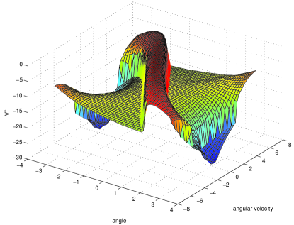
Figure 2: Optimal value function for the pendulum domain, computed with fitted value iteration over a discretized state space ($400\times 400$ grid).

6.1 Pendulum swing-up task

First, we consider the pendulum swing-up task, a common benchmark in RL. The goal is to swing up an underpowered pendulum and balance it around the inverted upright position (here formulated as an episodic task). More details and the equations of motion can be found in e.g. [5]. Since GPTD only solves (approximate) policy evaluation, to test our model selection approach we chose to generate a sample trajectory under the optimal policy (obtained from fitted value iteration). We generated a sequence of 1000 state-transitions under this policy (which corresponds to about 25 completed episodes) and applied GPTD for the three choices of covariance: isotropic (I), axis-aligned ARD (II), and factor analyis (III). In each case, the best setting of hyperparameters was found from running scaled conjugate gradients on Eq. (16), giving

I: $v_{0}=18.19$	$\sigma_{0}^{2}=0.05$	$b=0.11$	$h=7.48$
II: $v_{0}=15.95$	$\sigma_{0}^{2}=0.05$	$b=0.10$	$a_{1}=3.62$	$a_{2}=6.63$
III: $v_{0}=10.82$	$\sigma_{0}^{2}=0.08$	$b=0.10$	$s_{1}=13.91$	$s_{2}=0.36$	$\mathbf{u}_{1}=\begin{bmatrix}0.58&0.81\end{bmatrix}$	$\mathbf{u}_{2}=\begin{bmatrix}-0.81&0.58\end{bmatrix}$

(the last ones given in terms of the eigendecomposition of $\boldsymbol{\Omega}$). Figure 3 shows the results: all three produce an adequate representation of the true value function shown in Figure 2 in and near the states visited in the trajectory (MSE in states of the sample trajectory: (I) 0.27, (II) 0.24, and (III) 0.26), but differ once they start predicting values of states not in the training data (MSE for states on a $50\times 50$ grid: (I) 46.36, (II) 48.89, and (III) 12.24). Despite having a slightly higher error on the known training data, (III) substantially outperforms the other models when it comes to predicting the values of new states. With respect to model selection, (III) also has the highest likelihood. Note that (III) chooses one dominant direction ($\mathbf{u}_{1}=\begin{bmatrix}0.58&0.81\end{bmatrix}$) to which it assigns high relevance ($s_{1}=13.91$); the remainder ($\mathbf{u}_{2}=\begin{bmatrix}-0.81&0.58\end{bmatrix}$) has only little impact ($s_{2}=0.36$). Taking a closer look at Figure 2, we see that indeed the value function varies more strongly along the diagonal direction lower left to upper right, whereas it varies only slowly along the opposite diagonal upper left to lower right. For (II), relevance can only be assigned along the $\varphi$ and $\dot{\varphi}$ coordinates (state-variables), which in this case gives us no particular benefit; and (I) is not at all able to assign different importance to different state variables.

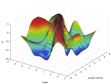
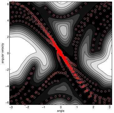
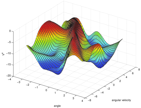
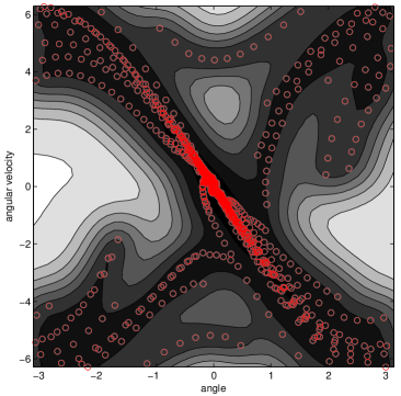
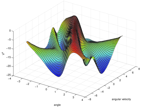
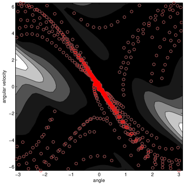
Figure 3: From top to bottom: GPTD approximation of the value function from Figure 2 for the covariances (I),(II),(III), where in each case the hyperparameters were obtained from marginal likelihood optimization for the GPTD process in Eq. (16). Right: Associated predictive variance. Black indicates low variance, white indicates high variance and red circles indicate the location of the states in the training set (which was the same for all three experiments).

Additional insight is gained by looking at the eigenspectrum of $\mathbf{K}$. Figure 4 (left) shows that (I)’s eigenvalues decrease the slowest, whereas (III)’s decrease the fastest. This has two consequences. First, the eigenspectrum is intimately related with complexity and generalization capabilities (see Eq. (16)) and thus helps explain why (III) delivers better prediction performance. Second, the eigenspectrum also indicates the effective rank of $\mathbf{K}$ and strongly impacts our ability to build an efficient low-rank approximation of $\mathbf{K}$ using as small a subset as possible (see Section 4). A small subset in turn is important for computational efficiency because its size is the dominant factor when we employ the SR-approximation: both for batch and online learning the operation count depends quadratically on the size of the subset (and only linear on the number of datapoints). Keeping this size as small as possible without losing predictive performance is essential. Figure 4 (center and right) shows that in this regard (III) performs best and (I) worst: for example, if we were to approximate $\mathbf{K}$ using SR-approximation with ICD selection at a tolerance level of $10^{-1}$, out of our 1000 samples (I) would choose $\sim 175$, (II) would chose $\sim 140$, and (III) would choose $\sim 80$ elements.

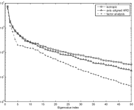
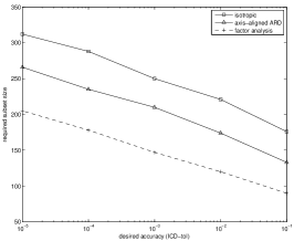
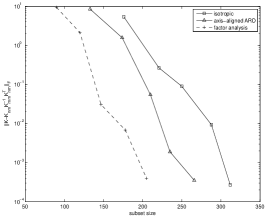
Figure 4: Properties of $\mathbf{K}$ for different choices of $k(\cdot,\cdot)$. Left: Eigenspectrum. Center: Number of elements incomplete Cholesky selects for a given threshold. Right: Approximation error $\left\|{\mathbf{K}-\tilde{\mathbf{K}}}\right\|_{F}$, given the size of the subset.

6.2 A 2D gridworld with 1 latent dimension

To illustrate in more detail how our approach handles irrelevant state variables, we use a specifically designed 2D gridworld with $11\times 11$ states. Every step entails a reward of $-1$ except when being in a state with $x=6$, which starts a new episode (teleports to a new random state with zero reward). We consider the policy that moves left when $x>6$ and right when $x<6$. In addition, every time we move left or right we will also move randomly up or down (with 50% each). The corresponding value function is shown in Figure 5 (left). We generated 500 transitions and applied GPTD with covariance (I) and (II) with automatic model selection resulting in

	Hyperparameters $\boldsymbol{\theta}$	Complexity	Data fit	$\mathcal{L}$ (smaller is better)
(I)	$\ h=2.89$	-2378.2	54.78	-2323.4
(II)	$\ a_{1}=3.53\quad a_{2}=10^{-5}\$	-2772.7	13.84	-2758.8
(II) without $y$	$\ a_{1}=3.53\quad a_{2}=0$	-2790.7	13.84	-2776.8

As can be seen from Figure 5 (center and right), both obtain a very reasonable approximation. However, (II) automatically detects that the $y$-coordinate of the state is irrelevant and thus assigns a very small weight to it ($a_{2}<10^{-5}$). With a uniform lengthscale, (I) is unable to do that and has to put equal weight on both state variables. As a consequence, its estimate is less exact and more wiggly (MSE: (I) 0.030, and (II) 0.019). Additional insight can be gained by looking at the likelihood $\mathcal{L}$ of the models (cf. Eq. (16)). Here we see that (II) has lower complexity (cf. eigenspectrum of $\mathbf{Q}$ in Figure 6), fits the data better and thus has a higher combined likelihood (note that the values in the table show the negative log likelihood which we minimize). Moreover, if we completely remove the $y$ state variable (setting $a_{2}:=0$), the eigenspectrum of $\mathbf{Q}$ decreases more rapidly; thus (II) without $y$ has an even lower complexity while still having the same fit. This indicates that state component $y$ can be safely ignored in this task/domain. In addition, as was mentioned before, the lower effective rank of $\mathbf{K}$ will also allow us to make more efficient use of SR-based approximations.

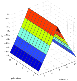
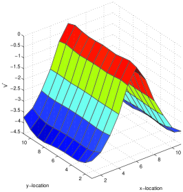
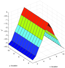
Figure 5: Learned value functions for the 2D-gridworld domain. Left: true value function. Note how the y-coordinate is irrelevant for the value. Center: approximation with isotropic covariance. Right: approximation for axis-aligned ARD covariance (after removal of irrelevant input).

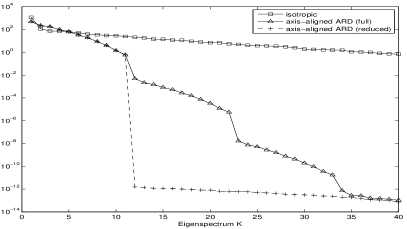
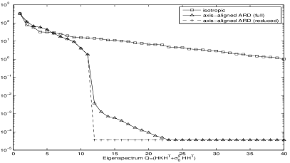
Figure 6: Effect of dimensionality reduction on the complexity of the model. Left: Eigenvalues of $\mathbf{K}$. Right: Eigenvalues of $\mathbf{Q}$.

7 Future work

It should be noted that the proposed framework for automatic feature generation and model selection should primarily be thought of as a practical tool: despite offering a principled solution to an important problem in RL, ultimately it does not come with any theoretical guarantees (due to some modeling assumptions from GPTD and the way the hyperparameters are obtained). For most practical applications this might be less of an issue, but in general care has to be taken.

The framework can be easily extended to perform policy evaluation over the joint state-action space to learn the model-free Q-function (instead of the V-function): we just have to choose a different covariance function, taking for example the product $k([\mathbf{x},a],[\mathbf{x}^{\prime},a^{\prime}])=k(\mathbf{x},\mathbf{x}^{\prime})k(a,a^{\prime})$ with $k(a,a^{\prime})=\delta_{a,a^{\prime}}$ for problems with a small number of discrete actions [8]. This opens the way for model-free policy improvement and thus optimal control via approximate policy iteration. Our next step then is to apply this approach to real-world high-dimensional control tasks, both in batch settings and hybrid batch/online settings; in the latter case exploiting the gain in computational efficiency obtained through model selection to improve [6].

References

- [1] F. R. Bach and M. I. Jordan. Kernel independent component analysis. JMLR, 3:1–48, 2002.
- [2] F. R. Bach and M. I. Jordan. Predictive low-rank decomposition for kernel methods. In Proc. of ICML 22, 2005.
- [3] D. Bertsekas. Dynamic programming and Optimal Control, Vol. II. Athena Scientific, 2007.
- [4] L. Csató and M. Opper. Sparse online Gaussian processes. Neural Computation, 14(3):641–668, 2002.
- [5] M. P. Deisenroth, C. E. Rasmussen, and J. Peters. Gaussian process dynamic programming. Neurocomputing, 72(7-9):1508–1524, 2009.
- [6] Y. Engel, S. Mannor, and R. Meir. Reinforcement learning with Gaussian processes. In Proc. of ICML 22, 2005.
- [7] S. Fine and K. Scheinberg. Efficient SVM training using low-rank kernel representation. JMLR, 2:243–264, 2001.
- [8] T. Jung and D. Polani. Learning robocup-keepaway with kernels. JMLR: Workshop and Conference Proceedings (Gaussian Processes in Practice), 1:33–57, 2007.
- [9] P. Keller, S. Mannor, and D. Precup. Automatic basis function construction for approximate dynamic programming and reinforcement learning. In Proc. of ICML 23, 2006.
- [10] Z. Luo and G. Wahba. Hybrid adaptive splines. J. Amer. Statist. Assoc., 92:107–116, 1997.
- [11] S. Mahadevan and M. Maggioni. Proto-value functions: A Laplacian framework for learning representation and control in Markov decision processes. JMLR, 8:2169–2231, 2007.
- [12] N. Menache, N. Shimkin, and S. Mannor. Basis function adaptation in temporal difference reinforcement learning. Annals of Operations Research, 134:215–238, 2005.
- [13] I. T. Nabney. Netlab : Algorithms for Pattern Recognition. Springer, 2002.
- [14] R. Parr, C. Painter-Wakefield, L. Li, and M. Littman. Analyzing feature generation for value-function approximation. In Proc. of ICML 24, 2007.
- [15] T. Poggio and F. Girosi. Networks for approximation and learning. Proceedings of the IEEE, 78(9):1481–1497, 1990.
- [16] C. E. Rasmussen and M. Kuss. Gaussian processes in reinforcement learning. In Advances in Neural Information Processing Systems 16, pages 751–759. MIT Press, 2004.
- [17] C. E. Rasmussen and C. K. I. Williams. Gaussian Processes for Machine Learning. MIT Press, 2006.
- [18] J. Reisinger, P. Stone, and R. Miikkulainen. Online kernel selection for Bayesian reinforcement learning. In Proc. of ICML 25, 2008.
- [19] M. Seeger, C. K. I. Williams, and N. Lawrence. Fast forward selection to speed up sparse Gaussian process regression. In Proc. of 9th Int’l Workshhop on AI and Statistics. Soc. for AI and Statistics, 2003.
- [20] E. Snelson and Z. Ghahramani. Sparse Gaussian processes using pseudo-inputs. In NIPS 18, 2006.
- [21] R. Sutton and A. Barto. Reinforcement Learning: An Introduction. MIT Press, 1998.
- [22] C. Williams and M. Seeger. Using the Nyström method to speed up kernel machines. In NIPS 13, pages 682–688, 2001.