Moving Target Parameters Estimation in Non-Coherent MIMO Radar Systems

Abstract

The problem of estimating the parameters of a moving target in multiple-input multiple-output (MIMO) radar is considered and a new approach for estimating the moving target parameters by making use of the phase information associated with each transmit-receive path is introduced. It is required for this technique that different receive antennas have the same time reference, but no synchronization of initial phases of the receive antennas is needed and, therefore, the estimation process is non-coherent. We model the target motion within a certain processing interval as a polynomial of general order. The first three coefficients of such a polynomial correspond to the initial location, velocity, and acceleration of the target, respectively. A new maximum likelihood (ML) technique for estimating the target motion coefficients is developed. It is shown that the considered ML problem can be interpreted as the classic “overdetermined” nonlinear least-squares problem. The proposed ML estimator requires multi-dimensional search over the unknown polynomial coefficients. The Cramér-Rao Bound (CRB) for the proposed parameter estimation problem is derived. The performance of the proposed estimator is validated by simulation results and is shown to achieve the CRB.

I Introduction

The detection and parameter estimation of moving targets is one of the most important radar applications [1]–[3]. The moving target parameters of interest can be the radar cross section (RCS), Doppler frequency, range/location, velocity, acceleration, etc. [2]. In conventional single antenna radar, the target RCS and range are measured from the amplitude and the time delay of the return signal, respectively, while the target velocity is measured from the Doppler frequency shift of the received signal [1]. The use of antenna arrays enables improving the signal strength resulting in improving the accuracy of target parameter estimation. In particular, antenna arrays are used at the transmitter to form/steer a beam towards a certain direction in space yielding coherent processing gain and at the receiver to coherently process the received data. A corresponding radar system is commonly referred to as phased-array radar [2]. However, it is well-known that phased-array radar suffers from RCS scintillations which are responsible for signal fading [4]. Therefore, a multiple-input multiple-output (MIMO) radar has recently become the focus of intensive research [5]–[9].

The essence of the MIMO radar concept is to employ multiple antennas for emitting several orthogonal waveforms and multiple antennas for receiving the echoes reflected by the target. MIMO radar can be either equipped with widely separated antennas [6] or colocated antennas [7]. The latter type employs arrays of closely spaced transmit/receive antennas which results in increasing the virtual aperture of the receive array due to the fact that multiple independent waveforms are received by the same receive array. This enables improving angular resolution, increasing the upper limit on the number of detectable targets, and improving parameter identifiability at the price of losing the transmit coherent processing gain offered by the phased-array radar [8]. On the other hand, a MIMO radar systems with widely separated transmit/receive antennas enable capturing the spatial diversity of the target’s RCS [6]. Capitalizing on the spatial diversity of the target, MIMO radar offers a potential to prevent RCS scintillation and to combat signal fading.

Several techniques are reported in the literature for target detection and localization in coherent MIMO radar systems [4], [10], [11]. However, the main focus of these techniques is to estimate the directions-of-arrival of targets located within a certain range-Doppler bin. The problem of estimating the location and/or velocity of a moving target is investigated in [12], [13]. However, in some practical applications the target may have variable speed which necessitates estimating not only the velocity but also the acceleration of the target. In this case, the target motion should be modeled as a second order polynomial. In other cases, even higher order polynomials for modeling the target motion have to be considered. For example, acceleration and jerk (rate of acceleration) are used to model the motion of agile maneuvering targets as described in [14], [15]. Note that for a maneuvering target, the radial velocity with respect to any single receiver exhibits variation which causes significant spread of the radar echo in the Doppler spectrum [16]. Other practical examples that exhibit variations in the target speed and, therefore, require high-order target motion modeling, include motion of highly maneuvering tactical ballistic missiles [17], landing of fighter jets on warship carriers [18], etc. Unfortunately, the variation in the target’s speed in the aforementioned applications limits the applicability of conventional techniques for target localization and parameter estimation.

In this work, we develop a maximum likelihood (ML) based estimator for estimating the parameters of a moving target in multi-static non-coherent MIMO radar systems. The radar motion within a certain processing interval is modeled as a general-order polynomial. In the specific case when the polynomial order is two, the polynomial coefficients correspond to the initial location, velocity, and acceleration of the target. By concentrating the ML function with respect to the nuisance parameters, e.g., reflection coefficients, we show that the ML problem can be interpreted in terms of the classic “overdetermined” nonlinear least-squares (LS) problem. The proposed ML estimator requires multi-dimensional search over the unknown parameters of interest, i.e., the unknown polynomial coefficients of the target motion. Simulation results demonstrate an excellent performance of the proposed estimator. It is worth noting that the superior performance of the proposed algorithm comes at price of the higher computational complexity mandated by the ML algorithm. Therefore, the development of a computationally efficient algorithms that enable reducing the computational cost of solving the proposed parameter estimation problem is of interest.

The rest of the paper is organized as follows. The MIMO radar signal model is given in Section II while the proposed moving target motion model is given in Section III. We derive the ML estimator in Section IV. The Cramér-Rao Bound (CRB) is derived in Section V. Simulation results which show the effectiveness of the proposed ML estimator are reported in Section VI followed by conclusions drawn in Section VII and Appendix where the details of CRB derivations are presented. This paper is reproducible research [20] and the software needed to generate the simulation results will be provided to the IEEE Xplore together with the paper upon its acceptance.

II MIMO Radar Signal Model

Consider a non-coherent MIMO radar system equipped with $M$ transmit and $N$ receive widely separated antennas. In a Cartesian three-dimensional (3D) space, the transmit and receive antennas are assumed to be located at ${\bf p}_{m}\triangleq[x_{m}\ y_{m}\ z_{m}]^{T},\ m=1,\ldots,M$ and ${\bf q}_{n}\triangleq[x_{n}\ y_{n}\ z_{n}]^{T},\ n=1,\ldots,N$, respectively, where $(\cdot)^{T}$ stands for the transpose operator. The complex envelope of the signal transmitted by the $m$-th transmitter can be written as

$$s_{m}(t)=\sqrt{\frac{E}{M}}\varphi_{m}(t),\quad 0\leq t\leq T$$ (1)

where $E$ is the total transmitted energy, $T$ is the radar pulse duration, $t$ is the time index within the radar pulse and $\varphi_{m}(t)$ is a unit-energy baseband waveform. Waveforms used at different transmitters are assumed to satisfy the orthogonality condition [12]

$$\int_{T}{\varphi}_{m}(t){\varphi_{i}}^{*}(t-\tau)dt=0,\quad{\rm for}\ m\neq i,\ \forall\tau$$ (2)

where $(\cdot)^{*}$ stands for the conjugate operator and $\tau$ is some time delay. Let ${\varphi}_{m}(t-\tau_{m})e^{-j2\pi f_{m}t}$ be a time-delayed frequency shifted version of ${\varphi}_{m}(t)$. Define the two-dimensional (2D) function $\chi_{m,i}(\tau,\nu)$ as

$$\chi_{m,i}(\tau,\nu) \!\!\!\triangleq\!\!\! \!\int_{T}\!{\varphi}_{m}\left(t\!-\!\tau_{m}\right)e^{-j2\pi f_{m}t}$$ (3)

$$\cdot{\varphi}_{i}^{*}(t\!-\!\tau)e^{j2\pi\nu t}dt.$$

where $\tau$ and $\nu$ are the time delay and frequency indexes, respectively. An important property of $\chi_{m,i}(\tau,\nu)$ is that

$$\max_{\tau,\nu}|\chi_{m,m}(\tau,\nu)|=1,\quad\tau=\tau_{m},\ \nu=f_{m}.$$ (4)

III Proposed Target Motion Model

Consider a moving target whose location during the $k$-th radar pulse is given in the 3D space by

$${\bf L}(k)=[x(k)\ y(k)\ z(k)]^{T},\quad k=1,\ldots,K$$ (5)

where $k$ is the slow time index (i.e. pulse number), and $K$ is the total number of radar pulses within a certain processing interval. In (5), $x(k)$, $y(k)$, and $z(k)$ are the $x$-, $y-$, and $z$-components of the target location, respectively. The target location during the $k$-th radar pulse can be described by the following $Q$-th order polynomials

$$x(k)=\sum_{q=0}^{Q}{C}_{q}\frac{(kT)^{q}}{q!},\quad k=0,\ldots,K$$ (6)

$$y(k)=\sum_{q=0}^{Q}{D}_{q}\frac{(kT)^{q}}{q!},\quad k=0,\ldots,K$$ (7)

$$z(k)=\sum_{q=0}^{Q}{E}_{q}\frac{(kT)^{q}}{q!},\quad k=0,\ldots,K$$ (8)

where $C_{q}$, $D_{q}$, and $E_{q}$ ($q=0,\ldots,Q$) are the unknown target motion coefficients and $\cdot!$ stands for the factorial of an integer. It is worth noting that for the mono-static radar, the use of (6)–(8) to model the target location results in a polynomial-phase signal (PPS) at the receiver and leads to the problem of PPS parameter estimation that has been extensively studied in the literature [21]–[23]. Note that the order of the PPS can be higher than two in the case when the carrier frequency at the transmitter is not constant (e.g., in the case when linear FM signals are used).

The complex envelope of the signal received by the $n$-th receiver can be written as

$${r}_{n}(t,k) \!\!\!\triangleq\!\!\! e^{j\phi_{n}}\sum_{m=1}^{M}\beta_{mn}{s_{m}}\left(t-\tau_{mn}(k)\right)e^{j2\pi f_{mn}(k)t}$$ (9)

$$\cdot\ e^{-j2\pi f_{c}\tau_{mn}(k)}\!+\!{w}(t,k),\;k=1,\!\ldots\!,K$$

where $\phi_{n}$ is the unknown initial phase of the $n$-th receiver, $\beta_{mn}$ is the target reflection coefficient associated with the $mn$-th transmit-receive path, $f_{mn}(k)$ is the Doppler frequency associated with the $mn$-th path during the $k$-th pulse, $f_{c}$ is the carrier frequency, ${w}(t,k)$ is the independent sensor noise which is assumed to be zero-mean white circularly Gaussian process, and $\tau_{mn}(k)$ is the time delay required for the carrier wave to travel through the $mn$-th transmit-receive path during the $k$-th pulse. We assume that the signal echoed from the target is present in the background of clutter plus noise. Moreover, we assume that the target can only migrate to an adjacent range-Doppler cell, and, therefore, the characteristics of the noise plus clutter component remains the same. If the clutter component is not Gaussian, space-time adaptive processing (STAP) can be used as a preprocessing step to filter out the clutter component [3]. Note that when the relative speed between the target and the radar platform is large, the fact that the spectrum of the clutter is centered around the platform velocity [24, Ch. 8] enables the use of STAP techniques to filter out the clutter. The time delay associated with the $(mn)$-th transmit-receive path can be defined as

$$\tau_{mn}(k)\triangleq\frac{\|{\bf L}(k)-{\bf p}_{m}\|+\|{\bf L}(k)-{\bf q}_{n}\|}{c}$$ (10)

where $c$ is the speed of light.

Using (2) and (4), the received signal (9) can be decomposed by matched-filtering the signal ${r}_{n}(t,k)$ to the waveforms ${\varphi}_{m}\left(t\!-\!\tau_{mn}(k)\right)e^{-j2\pi f_{mn}(k)t}$, yielding

$${r}_{mn}(k) \!\!\!\!=\!\!\!\! \!\sqrt{\frac{E}{M}}{\tilde{\beta}}_{mn}e^{-j2\pi f_{c}\tau_{mn}(k)}+w_{mn}(k)$$ (11)

where ${\tilde{\beta}}_{mn}\triangleq{\beta}_{mn}e^{j\phi_{n}}$ and $w_{mn}(k)$ is the noise component at the output of the matched filter. Note that the unknown initial phase component is absorbed in the unknown reflection coefficient. It is worth noting that it is assumed in (11) that range-Doppler cell synchronization [25] is performed before applying the matched-filtering step. More specifically, for each radar pulse, it is assumed that the range-Doppler cell that contains the target is known. We also assume that the time delay and the Doppler shift at which the matched-filter is performed coincide with the location of the peak of (4). In practice, the synchronized range-Doppler cell may slightly deviate from the location of the peak of (4). To account for the effect of such a deviation, the ambiguity function of the considered MIMO radar should be also considered [26].

The $MN\times 1$ virtual data vector can be formed as

$${\bf r}(k) \!\!\!\triangleq\!\!\! [{r}_{11}(k),\ldots,{r}_{MN}(k)]^{T}$$ (12)

$$\!\!\!=\!\!\! \sqrt{\frac{E}{M}}{\bf T}(k){\bf b}+{\bf w}(k)$$

where ${\bf T}(k)$ is a $MN\times MN$ diagonal matrix whose $mn$-th diagonal element is given by $e^{-j2\pi f_{c}\tau_{mn}(k)}$, ${\bf b}\triangleq[{\tilde{\beta}}_{11},\ldots,$ ${\tilde{\beta}}_{MN}]^{T}$ is $MN\times 1$ the vector of reflection coefficients, and ${\bf w}\triangleq[w_{11}(k),$ $\ldots,w_{MN}(k)]^{T}$ is the $MN\times 1$ virtual additive noise term. Note that each element of ${\bf w}(k)$ has the same statistics as $w_{mn}(k)$.

IV Maximum Likelihood Estimation

Let the $3(Q+1)\times 1$ vector of unknown coefficients associated with the moving target be defined as ${\boldsymbol{\psi}}=[C_{0},\ldots,\ C_{Q},$ $D_{0},\ldots,\ D_{Q},$ $E_{0},\ldots,\ E_{Q}]^{T}$. Assuming that the reflection coefficients associated with different transmit-receive paths are constant (deterministic) values, the virtual observations (12) satisfy the following statistical model:

$${\bf r}(k)\sim{\cal N}_{C}\left(\sqrt{\frac{E}{M}}{\bf T}(k){\bf b},\sigma^{2}{\boldsymbol{I}}\right)$$ (13)

where ${\cal N}_{C}$ denotes the complex multivariate circularly symmetric Gaussian probability density function, $\sigma^{2}$ is the noise variance, and ${\bf I}$ is the identity matrix.

Then, the negative log-likelihood (LL) function of the unknown parameters is given as

$${\mathcal{L}}({\boldsymbol{\psi}},{\bf b}) \!\!\!=\!\!\! \sum_{k=1}^{K}\left\|{\bf r}(k)-\sqrt{\frac{E}{M}}{\bf T}(k){\bf b}\right\|^{2}$$ (14)

$$\!\!\!=\!\!\! \sum_{k=1}^{K}{\bf r}^{H}(k){\bf r}(k)-\left(\sqrt{\frac{E}{M}}\sum_{k=1}^{K}{\bf r}^{H}(k){\bf T}(k)\right){\bf b}$$

$$-{\bf b}^{H}\left(\sqrt{\frac{E}{M}}\sum_{k=1}^{K}{\bf T}^{H}(k){\bf r}(k)\right)+{\bf b}^{H}\left(\frac{E}{M}\sum_{k=1}^{K}{\bf T}^{H}(k){\bf T}(k)\right){\bf b}.$$

The minimization of (14) over ${\bf b}$ yields

$$\hat{\bf b} \!\!\!=\!\!\! \sqrt{\frac{M}{E}}\left(\sum_{k=1}^{K}{\bf T}^{H}(k){\bf T}(k)\right)^{-1}\cdot\left(\sum_{k=1}^{K}{\bf T}^{H}(k){\bf r}(k)\right)$$ (15)

$$\!\!\!=\!\!\! \frac{1}{K}\sqrt{\frac{M}{E}}\sum_{k=1}^{K}{\bf T}^{H}(k){\bf r}(k)$$

where the second equality follows from the fact that $(\sum_{k=1}^{K}{\bf T}^{H}(k){\bf T}(k))^{-1}=1/K{\bf I}_{MN}$. It is worth noting that (15) can be used to compute the RCSs associated with different transmit-receive paths. This can be employed for reducing the dimensionality of the data by discarding the data associated with weak RCSs especially in the case of large values of $M$ and $N$. Substituting (15) into (14), we obtain

$${\mathcal{L}}({\boldsymbol{\psi}}) \!\!\!=\!\!\! \sum_{k=1}^{K}{\bf r}^{H}(k){\bf r}(k)$$ (16)

$$-\frac{1}{K}\left(\sum_{k=1}^{K}{\bf r}^{H}(k){\bf T}(k)\right)\cdot\left(\sum_{k=1}^{K}{\bf T}^{H}(k){\bf r}(k)\right).$$

The target parameters can be estimated by minimizing (16) over the unknown parameters. Alternatively, they can be obtained by maximizing the second term in (16). Therefore, the ML estimator can be defined as

$$\hat{\boldsymbol{\psi}}={\rm arg}\min_{\boldsymbol{\psi}}{\mathcal{L}}({\boldsymbol{\psi}})={\rm arg}\max_{\boldsymbol{\psi}}\left\|\sum_{k=1}^{K}{\bf T}^{H}(k){\bf r}(k)\right\|^{2}.$$ (17)

The above estimator jointly estimates the target parameters and generally requires a highly nonlinear optimization of (17) over ${\boldsymbol{\psi}}$. However, if properly initialized, the optimization of the LL function may be implemented by means of simple local optimization algorithms.

It is worth noting that the ML estimator can be recast in the form of the classic “overdetermined” nonlinear LS problem. Denoting $\tilde{\bf r}=[{\bf r}^{T}(1),\ldots,{\bf r}^{T}(K)]^{T}$ and ${\bf Q}=[{\bf T}^{T}(1),\ldots,{\bf T}^{T}(K)]^{T}$, we can rewrite (14) as

$${\cal L}({\boldsymbol{\psi}},{\bf b})=\left\|\tilde{\bf r}-\sqrt{\frac{E}{M}}{\bf Q}{\bf b}\right\|^{2}.$$ (18)

Minimizing (18) over ${\bf b}$ and substituting the result in (18), we obtain

$${\cal L}({\boldsymbol{\psi}})=\left\|{\bf P}^{\perp}_{{\bf Q}}{\bf y}\right\|^{2}=\tilde{\bf r}^{H}{\bf P}^{\perp}_{{\bf Q}}\tilde{\bf r}$$ (19)

where ${\bf P}^{\perp}_{{\bf Q}}={\bf I}-{\bf Q}({\bf Q}^{H}{\bf Q})^{-1}{\bf Q}^{H}$ is the orthogonal projection matrix onto the column subspace of ${\bf Q}$. Therefore, the ML estimator can be re-defined as

$$\hat{\boldsymbol{\psi}}={\rm arg}\min_{\boldsymbol{\psi}}\tilde{\bf r}^{H}{\bf P}^{\perp}_{{\bf Q}}\tilde{\bf r}={\rm arg}\max_{\boldsymbol{\psi}}\tilde{\bf r}^{H}{\bf Q}({\bf Q}^{H}{\bf Q})^{-1}{\bf Q}^{H}\tilde{\bf r}.$$ (20)

Note that (17) and (20) are equivalent. However, using (17) when optimizing the ML estimator is computationally more attractive than using (20) as it avoids computing the inverse of the $MN\times MN$ matrix ${\bf Q}^{H}{\bf Q}$.

Finding the ML estimation based on (17) is in general difficult and computationally demanding problem especially for large values of the polynomial order $Q$. Therefore, nonlinear optimization tools such as genetic algorithms, simulated annealing based methods, or expectation-maximization (EM)-type procedures can be used. However, good initialization of such algorithms is desirable to reduce the complexity. Here, we suggest a simple way for such an initialization. Particularly, we assume for initialization that each receive antenna can be used to obtain a coarse estimate of the target range at the discrete time instants $k=1,\ldots,K$. Then the coarse estimates to the target range with respect to different receive antennas can be used jointly to obtain a coarse estimate to the instantaneous target location $\hat{\bf L}(k),\ k=1,\ldots,K$. The range-only based target tracking approach reported in [27] can be, for example, used. Once, this coarse estimate is obtained, a simple polynomial regression can be performed to obtained the polynomial coefficients of the model. The so obtained estimates of the polynomial coefficients of the target model are then used as initial values for a specific optimization algorithm used.

V Cramér-Rao Bound

In this section, we give explicit expressions for the exact CRB on the accuracy of estimating the target model parameters. The $(2MN+3(Q+1))\times 1$ vector of unknown parameters (including reflection coefficients) can be defined as

$${\boldsymbol{\Psi}} \!\!\!=\!\!\! [{\boldsymbol{\psi}}_{x}^{T},{\boldsymbol{\psi}}_{y}^{T},{\boldsymbol{\psi}}_{z}^{T},{\rm Re}\{{\bf b}\}^{T},{\rm Im}\{{\bf b}\}^{T},\sigma^{2}]^{T}$$ (21)

$$\!\!\!=\!\!\! [{\boldsymbol{\psi}}^{T},\breve{\bf b}^{T},\sigma^{2}]^{T}$$

where ${\boldsymbol{\psi}}_{x}\triangleq[C_{0},\ldots,\ C_{Q}]^{T}$, ${\boldsymbol{\psi}}_{y}\triangleq[D_{0},\ldots,\ D_{Q}]^{T}$, ${\boldsymbol{\psi}}_{z}\triangleq[E_{0},\ldots,\ E_{Q}]^{T}$, ${\boldsymbol{\psi}}=[{\boldsymbol{\psi}}_{x}^{T},{\boldsymbol{\psi}}_{y}^{T},{\boldsymbol{\psi}}_{z}^{T}]^{T}$, and $\breve{\bf b}=[{\rm Re}\{{\bf b}\}^{T},{\rm Im}\{{\bf b}\}^{T}]^{T}$.

The elements of the FIM has the form of the complex circularly Gaussian process (13) can be expressed as

$${\bf F}=\frac{2E}{\sigma^{2}M}\cdot\begin{bmatrix}{\bf F}_{{\boldsymbol{\psi}}{\boldsymbol{\psi}}}&{\bf F}_{{\boldsymbol{\psi}}{\bf b}}\\ {\bf F}_{{\boldsymbol{\psi}}{\bf b}}^{H}&{\bf F}_{\breve{\bf b}\breve{\bf b}}\\ \end{bmatrix}$$ (22)

where the $3(Q+1)\times 3(Q+1)$ matrix ${\bf F}_{{\boldsymbol{\psi}}{\boldsymbol{\psi}}}$, the $3(Q+1)\times 2NM$ matrix ${\bf F}_{{\boldsymbol{\psi}}{\bf b}}$, and the $2NM\times 2NM$ matrix ${\bf F}_{\breve{\bf b}\breve{\bf b}}$ are defined as follows

$${\bf F}_{{\boldsymbol{\psi}}{\boldsymbol{\psi}}}={\rm Re}\left\{\sum_{k=0}^{K-1}\tilde{\bf B}^{H}(k)\tilde{\bf T}(k)^{H}\tilde{\bf T}(k)\tilde{\bf B}(k)\right\}$$ (23)

$${\bf F}_{{\boldsymbol{\psi}}{\bf b}}={\rm Re}\left\{\sum_{k=0}^{K-1}\tilde{\bf B}^{H}(k)\tilde{\bf T}(k)^{H}{\bf T}(k){\boldsymbol{J}}\right\}$$ (24)

$${\bf F}_{\breve{\bf b}\breve{\bf b}}={\rm Re}\left\{\sum_{k=0}^{K-1}{\boldsymbol{J}}^{H}{\bf T}^{H}(k){\bf T}(k){\boldsymbol{J}}\right\}.$$ (25)

Derivation of (23)–(25) and definitions of $\tilde{\bf B}^{H}(k)$, $\tilde{\bf T}(k)$, and ${\boldsymbol{J}}$ are given in Appendix.

Form (22), it follows that the CRB can be obtained as

$${\bf{CRB}} \triangleq \frac{\sigma^{2}}{2E/M}\cdot{\boldsymbol{F}}^{-1}.$$ (26)

From (26), we observe that the CRB on estimation performance is linearly proportional to the noise power and inversely proportional to the transmitted power per antenna, i.e., the CRB is directly proportional to the signal-to-noise ratio (SNR).

VI Simulation Results

In the first example, we assume that there are $M=3$ transmit antennas in a 2D plane located at $[(0,-5000),$  $\ (0,5000),$ $(5000,5000)]$m and there are $N=5$ receive antennas located at $[(0,-5000),$ $(0,0),$ $(0,5000),$ $(2500,5000),$ $(5000,5000)]$m. The motion of the target is parameterized by a second-order motion equation, i.e., by the initial location $(9800,$ $0)$m, velocity (100, 0)m/s, and acceleration $(-20,$ $0)$m/s². The radar pulse repetition time (PRT) used is $1.25$ms. The baseband (orthogonal) waveforms used at the three transmit antennas are exponential harmonics of the frequencies $1$ KHz, $2$ KHz, and $3$ KHz, respectively. The carrier frequency $f_{c}=300$ MHz is used at all transmit antennas and the propagation speed is assumed to be $3\times 10^{8}$ m/s. The transmitted energy $E$ is normalized so that $\sqrt{E/M}=1$. The $MN\times 1$ reflection coefficient vector is drawn randomly and then kept fixed throughout the simulations. The additive noise is modeled as a complex Gaussian zero-mean unit-variance spatially and temporally white process that has identical variances in each receive antenna. The whole observation time used in $0.5$s and is assumed to be divided into $Z=50,\ (Z<K)$ equally spaced intervals of width $0.01$s each, where $K$ was introduced earlier to denote the number of radar pulses. Each interval is assumed to be a coherent integration time (CIT), i.e., every CIT contains eight radar pulses. It is observed that the difference between the Doppler frequencies associated with the first and the last radar pulses within a certain CIT does not exceed $0.0013$ Hz for all CITs within the whole observation time. Therefore, it can be assumed that the Doppler frequency does not change during the same CIT but changes from CIT to CIT. The ML estimator (17) is used to estimate the target parameters. Instead of finding the minimum of (19), we search for the peak of the positive LL function

$${\cal L}_{p}({\boldsymbol{\psi}})={\bf y}^{H}{\bf P}_{{\bf Q}}{\bf y}$$ (27)

where ${\bf P}_{{\bf Q}}\triangleq{\bf Q}({\bf Q}^{H}{\bf Q})^{-1}{\bf Q}^{H}$. The genetic algorithm (GA) is used to optimize ${\cal L}_{p}({\boldsymbol{\psi}})$ over the unknown parameters $C_{q}$, $q=0,\ 1,\ 2$, i.e., the unknown target initial location, velocity, and acceleration. To make sure that the estimation accuracy is not limited by the size of the search region, the boundaries of the GA search region, for each parameter, are taken wide enough ($20$ times larger than the corresponding CRB) and centered at the true values. The root mean-square errors (RMSEs) are computed for the parameters of interest based on $100$ independent simulation runs. The RMSEs of the estimates of the unknown parameters are compared to the corresponding CRBs.

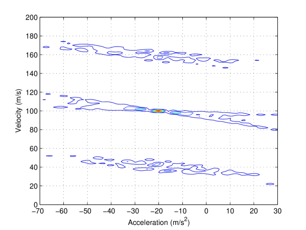
Figure 1: Contour plot of the ML function (20) in the velocity-acceleration plane; example 1.

Fig. 1 shows the contour plot of (17) computed in the 2D velocity-acceleration plane while the initial location is fixed to its true value. The SNR for this case is fixed to $0$ dB. It can be seen from this figure that the ML estimator exhibits main peak close to the true values of both the velocity and acceleration parameters. Two other 2D contour plots computed in the location-velocity and location-acceleration planes exhibit similar behavior as that in Fig. 1. The location-velocity and location-acceleration contour plots are similar.

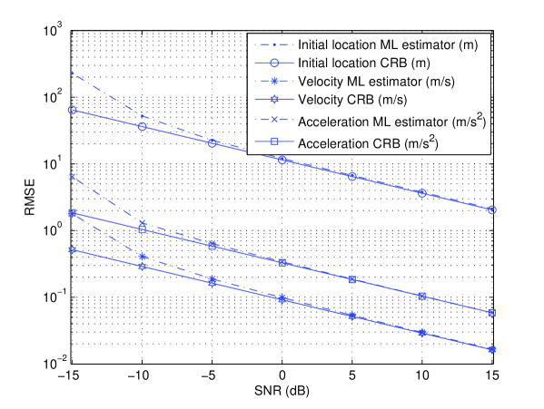
Figure 2: RMSEs versus SNR; example 1.

Fig. 2 shows the RMSEs versus SNR for the initial location, velocity and acceleration. It can be seen from the figure that the initial location estimation accuracy is in the range of tens of meters at SNR values below $0$ dB and it is in the range of meters at SNR values above $0$ dB. Also, it can be observed from the figure that the RMSEs for the initial location, velocity, and acceleration estimation coincide with the CRB at moderate and high SNR regions. It is clear from Fig. 2 that the proposed ML estimator offers excellent estimation accuracy for estimating the target location, velocity, and acceleration.

In the second example, we show that the proposed method is also applicable to the case of fixed speed targets. In this case, the target motion is described by a first-order polynomial where the initial location of the target is taken as $(8400,$ $9800)$m and the target velocity is assumed to be (40, -50)m/s. The transmit antennas are located at $[(0,0),$  $\ (4000,0),$ $(0,4000)]$m and the receive antennas are located at $[(0,0),$ $(2000,0),$ $(0,2000),\ (6000,0),$ $(0,6000)]$m. The radar pulse width and the waveforms used at the transmitters are the same as in the first example. The overall observation duration is $2.0$s. Noting that the target speed is constant, the Doppler frequency is the same during the whole observation time which enables using longer CITs. The observation time is divided into $K=50$ equally spaced intervals of duration $0.04$s each. Each CIT involves energy integration over $32$ radar pulses. Similar to the previous example, the GA initialized around the true parameters is used to optimize the LL function over the unknown initial location and target velocity components.

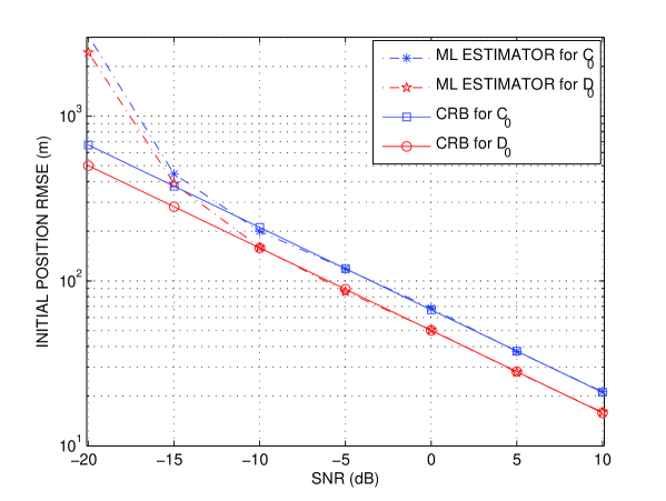
Figure 3: Initial position estimation RMSEs versus SNR; example 2.

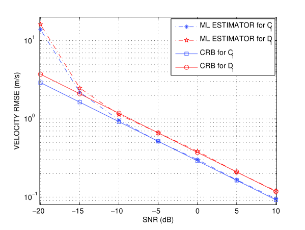
Figure 4: Velocity estimation RMSEs versus SNR; example 2.

Fig. 3 shows the RMSEs versus SNR for the $x$- and the $y$-components of the target initial location. It can be seen from this figure that the performance of the proposed ML method coincides with the CRB for SNR values higher than $-10$ dB. Fig. 4 shows the RMSEs versus SNR for the $x$- and the $y$-components of the target velocity. It can be seen from the figure that the proposed ML method has excellent velocity estimation performance which coincides with the CRB as the SNR increases.

VII Conclusions

A new ML estimator for moving target parameter estimation in non-coherent MIMO radar has been developed. The target motion within a certain processing interval is modeled as a general-order polynomial which is suitable for modeling the motion of a moving target with rapidly changing speed such as a jet landing on an aircraft carrier. The ML function is concentrated with respect to the nuisance parameters (target reflection coefficients). The resulting ML estimator requires a multi-dimensional search over the unknown parameters of interest (coefficients of the target motion model). It has been shown that the proposed ML approach can be interpreted in the form of the classic “overdetermined” nonlinear LS problem. The performance of the proposed ML estimator is validated by simulations and it is shown that it achieves the CRB derived for the considered parameter estimation problem.

Appendix: Computation of the Fisher Information Matrix

The elements of the FIM of a complex circularly Gaussian process ${\bf x}(k)\sim{\cal N}_{C}\left({\boldsymbol{\mu}}(k),{\boldsymbol{R}}\right)$ are given by [28]

$$\left[{\boldsymbol{F}}\right]_{i,j} = N\,{\rm trace}\left\{{\boldsymbol{R}}^{-1}\frac{\partial{\boldsymbol{R}}}{\partial\Psi_{i}}{\boldsymbol{R}}^{-1}\frac{\partial{\boldsymbol{R}}}{\partial\Psi_{j}}\right\}$$ (28)

$$+\,2\,{\rm Re}\left\{\sum_{k=0}^{K-1}\frac{\partial{\boldsymbol{\mu}}^{H}(k)}{\partial\Psi_{i}}{\boldsymbol{R}}^{-1}\frac{\partial{\boldsymbol{\mu}}(k)}{\partial\Psi_{j}}\right\}$$

where $\Psi_{i}$ is the $i$-th element of ${\boldsymbol{\Psi}}$. Applying (28) to the model (13), we obtain

$$\left[{\boldsymbol{F}}\right]_{i,j} = \frac{KNM}{\sigma^{4}}\,\frac{\partial\sigma^{2}}{\partial\Psi_{i}}\,\frac{\partial\sigma^{2}}{\partial\Psi_{j}}$$ (29)

$$+\,\frac{2E}{\sigma^{2}M}{\rm Re}\left\{\sum_{k=0}^{K-1}\frac{\partial\left\{{\bf b}^{H}{\bf T}^{H}(k)\right\}}{\partial\Psi_{i}}\cdot\,\frac{\partial\left\{{\bf T}(k){\bf b}\right\}}{\partial\Psi_{j}}\right\}$$

Direct computation yields,

$$\frac{\partial\left\{{\bf b}^{H}{\bf T}^{H}(k)\right\}}{\partial{\rm Re}\{{\bf b}\}} = {\bf T}^{H}(k)$$ (30)

$$\frac{\partial\left\{{\bf b}^{H}{\bf T}^{H}(k)\right\}}{\partial{\rm Im}\{{\bf b}\}} = -j{\bf T}^{H}(k).$$ (31)

Introducing the $NM\times 2NM$ matrix ${\boldsymbol{J}}=[{\boldsymbol{I}},j{\boldsymbol{I}}]$, we can rewrite (30) and (31) in a compact form as

$$\frac{\partial\left\{{\bf b}^{H}{\bf T}^{H}(k)\right\}}{\partial\breve{\bf b}}={\boldsymbol{J}}^{H}{\bf T}^{H}(k).$$ (32)

Eq. (10) can be rewritten as

$$\tau_{mn}(kT)\triangleq\frac{d_{m}+d_{n}}{c}$$ (33)

where

$$d_{m} = \left[\left(\sum_{q=0}^{Q}{C}_{q}\frac{(kT)^{q}}{q!}-x_{m}\right)^{2}\right.$$ (34)

$$\left.+\left(\sum_{q=0}^{Q}{D}_{q}\frac{(kT)^{q}}{q!}-y_{m}\right)^{2}+\left(\sum_{q=0}^{Q}{E}_{q}\frac{(kT)^{q}}{q!}-z_{m}\right)^{2}\right]^{1/2}$$

$$d_{n} = \left[\left(\sum_{q=0}^{Q}{C}_{q}\frac{(kT)^{q}}{q!}-x_{n}\right)^{2}\right.$$ (35)

$$\left.+\left(\sum_{q=0}^{Q}{D}_{q}\frac{(kT)^{q}}{q!}-y_{n}\right)^{2}+\left(\sum_{q=0}^{Q}{E}_{q}\frac{(kT)^{q}}{q!}-z_{n}\right)^{2}\right]^{1/2}.$$

Straightforward computations yield

$$\frac{\partial\left\{e^{-j2\pi f_{c}\tau_{mn}(kT)}\right\}}{\partial C_{0}} \!\!\!=\!\!\! \frac{\partial\left\{e^{-j2\pi f_{c}\tau_{mn}(kT)}\right\}}{\partial\tau_{mn}(kT)}\cdot\frac{\partial\tau_{mn}(kT)}{\partial C_{0}}$$ (36)

$$\!\!\!=\!\!\! \left\{-j2\pi f_{c}e^{-j2\pi f_{c}\tau_{mn}(kT)}\right\}$$

$$\cdot\frac{1}{c}\left(\frac{\sum_{q=0}^{Q}{C}_{q}\frac{(kT)^{q}}{q!}-x_{m}}{d_{m}}+\frac{\sum_{q=0}^{Q}{C}_{q}\frac{(kT)^{q}}{q!}-x_{n}}{d_{n}}\right)$$

Therefore, we obtain

$$\frac{\partial\left\{{\bf b}^{H}{\bf T}^{H}(k)\right\}}{\partial C_{0}} \!\!\!=\!\!\! {\bf b}^{H}\left({\bf T}(k)\odot{\bf Z}_{x}(k)\right)^{H}$$ (37)

where the $MN\times MN$ diagonal matrix ${\bf Z}_{x}(k)$ is given by

$$[{\bf Z}_{x}(k)]_{nM+m,nM+m} \!\!\!=\!\!\! \frac{-j2\pi f_{c}}{c}\left(\frac{\sum_{q=0}^{Q}{C}_{q}\frac{(kT)^{q}}{q!}-x_{m}}{d_{m}}\right.$$ (38)

$$\left.+\frac{\sum_{q=0}^{Q}{C}_{q}\frac{(kT)^{q}}{q!}-x_{n}}{d_{n}}\right)$$

Similar computations yield

$$\frac{\partial\left\{{\bf b}^{H}{\bf T}^{H}(k)\right\}}{\partial C_{q}} \!\!\!=\!\!\! \frac{(kT)^{q}}{q!}{\bf b}^{H}\left({\bf T}(k)\odot{\bf Z}_{x}(k)\right)^{H},\quad q=1,\ldots,Q.$$ (39)

Introducing the $(Q+1)\times 1$ vector ${\bf h}\triangleq[1,\ldots,\ \frac{(kT)^{Q}}{q!}]^{T}$, we can define the $2NM\times(Q+1)$ matrix

$${\bf B}(k)={\bf h}^{T}\otimes{\bf b}.$$ (40)

Therefore, we obtain

$$\frac{\partial\left\{{\bf b}^{H}{\bf T}^{H}(k)\right\}}{\partial{\boldsymbol{\psi}}_{x}} \!\!\!=\!\!\! {\bf B}^{H}(k)\tilde{\bf T}^{H}_{x}(k).$$ (41)

where $\tilde{\bf T}_{x}(k)\triangleq{\bf T}(k)\odot{\bf Z}_{x}(k)$.

Following the same steps, we obtain

$$\frac{\partial\left\{{\bf b}^{H}{\bf T}^{H}(k)\right\}}{\partial{\boldsymbol{\psi}}_{y}} \!\!\!=\!\!\! {\bf B}^{H}(k)\tilde{\bf T}^{H}_{y}(k).$$ (42)

where $\tilde{\bf T}_{y}(k)\triangleq{\bf T}(k)\odot{\bf Z}_{y}(k)$ and the $MN\times MN$ diagonal matrix ${\bf Z}_{y}(k)$ is given by

$$[{\bf Z}_{y}(k)]_{nM+m,nM+m} \!\!\!=\!\!\! \frac{-j2\pi f_{c}}{c}\left(\frac{\sum_{q=0}^{Q}{D}_{q}\frac{(kT)^{q}}{q!}-y_{m}}{d_{m}}\right.$$ (43)

$$\left.+\frac{\sum_{q=0}^{Q}{D}_{q}\frac{(kT)^{q}}{q!}-y_{n}}{d_{n}}\right).$$

Similarly, we have

$$\frac{\partial\left\{{\bf b}^{H}{\bf T}^{H}(k)\right\}}{\partial{\boldsymbol{\psi}}_{z}} \!\!\!=\!\!\! {\bf B}^{H}(k)\tilde{\bf T}^{H}_{z}(k).$$ (44)

where $\tilde{\bf T}_{z}(k)\triangleq{\bf T}(k)\odot{\bf Z}_{z}(k)$ and the $MN\times MN$ diagonal matrix ${\bf Z}_{z}(k)$ is given by

$$[{\bf Z}_{z}(k)]_{nM+m,nM+m} \!\!\!=\!\!\! \frac{-j2\pi f_{c}}{c}\left(\frac{\sum_{q=0}^{Q}{E}_{q}\frac{(kT)^{q}}{q!}-z_{m}}{d_{m}}\right.$$ (45)

$$\left.+\frac{\sum_{q=0}^{Q}{E}_{q}\frac{(kT)^{q}}{q!}-z_{n}}{d_{n}}\right).$$

Introducing the matrix ${\tilde{\bf B}(k)}\triangleq{\bf I}_{3}\otimes{\bf B}(k)$ and the matrix $\tilde{\bf T}(k)=[\tilde{\bf T}_{x}(k),\ \tilde{\bf T}_{y}(k),\ \tilde{\bf T}_{z}(k)]$, we obtain

$$\frac{\partial\left\{{\bf b}^{H}{\bf T}^{H}(k)\right\}}{\partial{\boldsymbol{\psi}}} \!\!\!=\!\!\! \tilde{\bf B}^{H}(k)\tilde{\bf T}^{H}(k).$$ (46)

Substituting (32) and (46) in (29), the expressions that define the FIM in (22)–(25) are readily obtained.

References

- [1] G. R. Curry, Radar System Performance Modeling, 2nd ed. Boston: Artech House, 2005.
- [2] M. I. Skolnik, Introduction to Radar Systems, 3rd ed. New York: McGraw-Hill, 2001.
- [3] R. Klemm, Applications of Space-Time Adaptive Processing, London, UK: IEE Press, 2004.
- [4] N. Lehmann, E. Fishler, A. Haimovich, R. Blum, D. Chizhik, L. Cimini, and R. Valenzuela, “Evaluation of transmit diversity in MIMO-radar direction finding,” IEEE Trans. Signal Processing, vol. 55, pp. 2215–2225, May 2007.
- [5] E. Fishler, A. Haimovich, R. Blum, D. Chizhik, L. Cimini, and R. Valenzuela, “MIMO radar: An idea whose time has come,” in Proc. IEEE Radar Conf., Honolulu, Hawaii, USA, Apr. 2004, vol. 2, pp. 71–78.
- [6] A. Haimovich, R. Blum, and L. Cimini, “MIMO radar with widely separated antennas,” IEEE Signal Processing Mag., vol. 25, pp. 116–129, Jan. 2008.
- [7] J. Li and P. Stoica, “MIMO radar with colocated antennas,” IEEE Signal Processing Magazine, vol. 24, pp. 106–114, Sept. 2007.
- [8] F. Daum and J. Huang, “MIMO radar: Snake oil or good idea,” IEEE Aerosp. Electron. Syst. Magazine, pp. 8–12, May 2009.
- [9] A. Hassanien and S. A. Vorobyov, “Transmit energy focusing for DOA estimation in MIMO radar with colocated antennas,” IEEE Trans. Signal Processing, vol. 59, no. 6, pp. 2669–2682, June 2011.
- [10] I. Bekkerman and J. Tabrikian, “Target detection and localization using MIMO radars and sonars,” IEEE Trans. Signal Processing, vol. 54, pp. 3873–3883, Oct. 2006.
- [11] L. Xu, J. Li, and P. Stoica, “Target detection and parameter estimation for MIMO radar systems,” IEEE Trans. Aerosp. Electron. Syst., vol. 44, no. 3, pp. 927–939, July 2008.
- [12] Q. He, R. S. Blum, H. Godrich, and A. M. Haimovich, “Cramer-Rao bound for target velocity estimation in MIMO radar with widely separated antennas,” in Proc. 42nd Annual Conf. Information Sciences and Systems (CISS’08), Princeton, NJ, Mar. 2008, pp. 123–127.
- [13] Q. He, R. S. Blum, and A. M. Haimovich, “Noncoherent MIMO radar for location and velocity estimation: More antennas means better performance,” IEEE Trans. Signal Processing, vol. 58, no. 7, pp. 3661–3680, Jul. 2010.
- [14] P. Mahapatra and K. Mehrotra, “Mixed coordinate tracking of generalized maneuvering targets using acceleration and jerk models,” IEEE TTrans. Aerosp. Electron. Syst., vol. 36, no. 3, pp. 992–1000, Jul. 2000.
- [15] K. Mehrotra and P. Mahapatra, “A jerk model for tracking highly maneuvering targets,” IEEE Trans. Aerosp. Electron. Syst., vol .33, no .4, pp. 1094–1105, Oct. 1997.
- [16] K. Lu and X. Liu, “Enhanced visibility of maneuvering targets for high-frequency over-the-horizon radar,” IEEE Trans. Antennas and Propagation, vol. 53, no. 1, pp. 404–411, Jan. 2005.
- [17] J. Shinar and T. Shima, “Robust missile guidance law against highly maneuvering targets,” in Proc. 7th Mediterranean Conf. Control and Automation (MED99) Haifa, Israel, June 1999, pp. 1548–1572.
- [18] R. A. Richards, “Application of multiple artificial intelligence techniques for an aircraft carrier landing decision support tool,” in Proc. IEEE Int. Conf. on Fuzzy Systems, May 2002, pp. 7–11.
- [19] A. Hassanien, S. A. Vorobyov, A. B. Gershman, and M. Ruebsamen, “Estimating the parameters of a moving target in MIMO radar with widely separated antennas,” invited paper, in Proc. 6th IEEE Workshop Sensor Array and Multichannel Signal Processing, SAM’10, Israel, Oct. 2010, pp. 57–60.
- [20] P. Vandewalle, J. Kovacevic, and M. Vetterli, “Reproducible research in signal processing,” IEEE Signal Process. Magazine, vol. 26, no. 3, pp. 37–47, May 2009.
- [21] S. Barbarossa, A. Scaglione, and G. B. Giannakis, “Product high-order ambiguity function for multicomponent polynomial-phase signal modeling,” IEEE Trans. Signal Processing, vol. 46, pp. 691–708, Mar. 1998.
- [22] F. Gini and G. B. Giannakis, “Hybrid FM-polynomial phase signal modeling: Parameter estimation and Cramer-rao bounds,” IEEE Trans. Signal Processing, vol. 47, pp. 363–377, Feb. 1999.
- [23] F. Gini, M Montanari, and L. Verrazzani, “Estimation of chirp radar signal in compound-Gaussian clutter: A cyclostationary approach,” IEEE Trans. Signal Processing, vol. 48, pp. 1029–1039, Apr. 2000.
- [24] M. A. Richards, J. A. Scheer, and W. A. Holm, Edrs Principles of Modern Radar: Basic Principles, 2nd ed. Raleigh, NC: SciTech, 2010.
- [25] A. De Maio, M. Lops, and L. Venturino, “Diversity-integration tradeoffs in MIMO detection,” IEEE Trans. Signal Processing, vol. 56, no. 10, pp. 5051–5061, Oct. 2008.
- [26] G. San Antonio, D. R. Fuhrmann, F .C. Robey, “MIMO radar ambiguity functions,” IEEE J. Selected Topics in Signal Processing, vol. 1, no. 1, pp. 167–177, June 2007.
- [27] G. L. Soares, A. Arnold-Bos, L. Jaulin, C. A. Maia, and J. A. Vasconcelos, “An interval-based target tracking approach for range-only multistatic radar,” IEEE Trans. Magnetics, vol. 44, no. 6, pp. 1350–1353, June 2008.
- [28] P. Stoica and A. Nehorai, “Performance study of conditional and unconditional direction-of-arrival estimation,” IEEE Trans. Acoust., Speech, Signal Processing, vol. 38, pp. 1783–1795 , Oct. 1990.