Quantitative analysis of quantum phase slips in superconducting Mo₇₆Ge₂₄ nanowires
revealed by switching-current statistics

Abstract

We measure quantum and thermal phase-slip rates using the standard deviation of the switching current in superconducting nanowires. Our rigorous quantitative analysis provides firm evidence for the presence of quantum phase slips (QPSs) in homogeneous nanowires at high bias currents. We observe that as temperature is lowered, thermal fluctuations freeze at a characteristic crossover temperature $T_{q}$, below which the dispersion of the switching current saturates to a constant value, indicating the presence of QPSs. The scaling of the crossover temperature $T_{q}$ with the critical temperature $T_{c}$ is linear, $T_{q}\propto T_{c}$, which is consistent with the theory of macroscopic quantum tunneling. We can convert the wires from the initial amorphous phase to a single-crystal phase, in situ, by applying calibrated voltage pulses. This technique allows us to probe directly the effects of the wire resistance, critical temperature, and morphology on thermal and quantum phase slips.

I Introduction

Topological fluctuations of the order parameter field, so-called Little’s phase slips, Little1 are at the heart of superconductivity at the nanoscale. Tinkham ; AGZ-Review ; Bezryadin-Review These unavoidable stochastic events give rise to the finite resistivity of nanowires below the mean-field transition temperature. Thermally activated phase slips (TAPSs) have been routinely observed experimentally; see Ref. Bezryadin-Review, for a review. However, at low temperatures, phase-slip events are triggered by intrinsic quantum fluctuations, MDC-PRB87 ; Giordano ; Sahu-NatPhys09 so they are called quantum phase slips (QPSs) and represent a particular case of macroscopic quantum tunneling (MQT). A clear and unambiguous demonstration of MQT in homogeneous superconductors is of great importance, from both the fundamental and the technological prospectives. It has been argued recently by Mooij and Nazarov MN-NatPhys06 that a wire where coherent QPSs take place may be regarded as a new circuit element, the phase-slip junction, which is a dual counterpart of the Josephson junction. Pop-NatPhys10 The proposed phase-slip qubit MH-NJP05 and other coherent devices MN-NatPhys06 ; HN-PRL11 ; Zorin-PRL12 ; Astafiev-NP12 may be useful in the realization of a new current standard. Furthermore, comprehensive study of QPSs may elucidate the microscopic nature of superconductor-insulator quantum phase transition in nanowires. Dynes ; BezryadinNature ; Shahar ; Bollinger1

It is difficult to obtain firm conclusions about the presence of QPSs by means of low-bias resistance measurements because the resistance drops to zero at relatively high temperatures. Measured in the linear transport regime, high-resistance wires seemingly exhibit QPSs, Lau while low-resistance wires probably do not. Bollinger2 For high-bias currents, on the other hand, Sahu et al. Sahu-NatPhys09 obtained strong evidence supporting the quantum nature of phase slips by measuring switching-current distributions. The observed drop of the switching-current dispersion with increasing temperature was explained by a delicate interplay between quantum and multiple thermal phase slips. Recently Li et al. Li-PRL11 provided direct experimental evidence that, at sufficiently low temperatures, each phase slip causes nanowire switching from superconducting to the normal state by creating a hot spot. Sahu-NatPhys09 ; Shah-PRL07 The destruction of superconductivity occurs by means of overheating the wire caused by a single phase slip. Thus the dispersion of phase-slip events is equivalent to the dispersion of the switching current.

We build on these previous findings and reveal MQT in homogeneous nanowires via the quantitative study of current-voltage characteristics. First, we examine the higher-temperature regime, $T_{q}<T<T_{c}$, and identify thermal phase slips through the temperature dependence of the switching-current standard deviation $\sigma$, which obeys the 2/3 power law predicted by Kurkijärvi. Kurkijarvi At lower temperatures, $T<T_{q}$, a clear saturation of $\sigma$ is observed; this behavior is indicative of MQT. Important evidence in favor of QPSs is provided by the fact that the mean value of the switching current keeps increasing with cooling even when the associated dispersion is already saturated. We observe a linear scaling of the saturation temperature $T_{q}$ with the critical temperature $T_{c}$ of the wire. We also show that such behavior is in agreement with our generalization of the MQT theory. This fact provides extra assurance that other mechanisms, such as electromagnetic (EM) noise or inhomogeneities, are not responsible for the observed behavior. Furthermore, we achieve controllable tunability of the wire morphology by utilizing a recently developed voltage pulsation technique. Aref-NanoTech11 The pulsation allows us to gradually crystallize the wire and to change its $T_{c}$ in situ. The fact that the QPS manifestations are qualitatively the same in both amorphous and crystallized wires eliminates the possibility that the observed MQT behavior is caused by the presence of weak links. Thus we provide conclusive evidence for the existence of QPSs in homogeneous wires in the nonlinear regime of high-bias currents.

II Experimental details

Superconducting nanowires were fabricated by molecular templating. BezryadinNature ; Bezryadin-Review Briefly, a single-wall carbon nanotube is suspended across a trench etched in a silicon wafer. The nanotube and the entire surface of the chip are then coated with 10-20 nm of the superconducting alloy Mo₇₆Ge₂₄ using dc magnetron sputtering. Thus a nanowire, seamlessly connected to thin film electrodes at its ends, forms on the surface of the electrically insulating nanotube. The electrodes approaching the wire are between $5$ and $20~{}\mu$m wide. The gap between the electrodes, in which the nanowire is located, is 100 nm.

The signal lines in the He-3 cryostat were heavily filtered to eliminate electromagnetic noise, using copper-powder and silver-paste filters at low temperatures and $\pi$ filters at room temperature. MDC-PRB87 To measure switching-current distributions, the bias current was gradually increased from zero to a value that is about 20% higher than the critical current (1-10 $\mu$A). Such large sweeps ensure that each measured $I$-$V$ curve exhibits a jump from the zero-voltage state to the resistive normal state. Such a jump is defined as the switching current $I_{sw}$, and $N=10^{4}$ switching events were detected at each temperature through repetitions of the $I$-$V$ curve measurements $N$ times. The standard deviation (i.e., dispersion) $\sigma$ and the mean value $\langle I_{sw}\rangle$ are computed in the standard way.

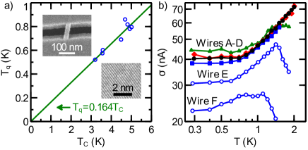
Figure 1: [Color online] (a) The saturation temperature $T_{q}$ vs the critical temperature $T_{c}$ for samples A-D, pulsed and unpulsed. The line is the best fit. The top insert shows SEM image of an unpulsed nanowire; the bottom insert shows a TEM micrograph of a nanowire crystallized by applying voltage pulses. Aref-NanoTech11 The fringes corresponding to atomic planes are visible. (b) The standard deviation of the switching current versus temperature, for samples A-F (prior to any pulsing).

We apply strong voltage pulses to induce Joule heating, which crystallizes our wires [see bottom inset in Fig. 1(a)] and also changes their critical temperature $T_{c}$. Aref-NanoTech11 With increasing pulse amplitude, $T_{c}$ (as well as $I_{c}$) initially diminishes and then increases back to the starting value or even exceeds it in some cases. Such modifications of $T_{c}$ and $I_{c}$ have been explained by morphological changes, as the amorphous molybdenum germanium (Mo₇₆Ge₂₄) gradually transforms into single-crystal Mo₃Ge, caused by the Joule heating brought about by the voltage pulses. The return of $T_{c}$ and $I_{c}$ is accompanied by a drop in the normal resistance $R_{n}$ of the wire, which is caused by the crystallization and the corresponding increase of the electronic mean free path. The pulsing procedure allows us to study the effect of $T_{c}$ on $T_{q}$ [see Fig. 1(a)] and the effect of the morphology of the wire on the QPS process in general. Note that after the pulsing is done and the morphology of the wire is changed in the desired way, we always allow a sufficient time for the wire to return to the base temperature before measuring $I_{sw}$.

III Results, Analysis and Modeling

Current-voltage characteristics for our wires display clear hysteresis, sustained by Joule heating, similar to Refs. Sahu-NatPhys09, ; Bollinger1, ; Tinkham-PRB03, . The switching current from dissipationless branch to resistive branch of the $I$-$V$ curve fluctuates from one measurement to the next, even if the sample and the environment are unchanged. Examples of the distributions of the switching current are shown in Fig. 2(a) for different temperatures. Since, by definition, the area under each distribution is constant, the fact that at $T<0.7\,$K its height stops increasing with cooling implies that its width, which is proportional to $\sigma$, is constant as well; see Fig. 1(b). Thus we get the first indication that the quantum regime exists for $T<0.7\,$K, i.e. for this case $T_{q}\approx 0.7\,$K.

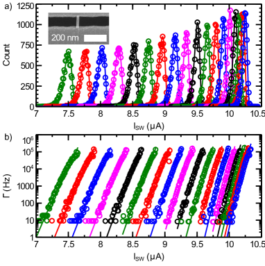
Figure 2: [Color online] Distributions and the switching rates for wire A. (a) Measured switching current distributions (circles) for various temperatures ranging from 2 K for the left curve to 0.3 K for the right curve (step = 0.1 K). The fits are shown as solid lines of the same color. Gumbel The inset shows a SEM image of a representative nanowire after completing the pulsing procedure. (b) Switching rates, derived from the distribution shown in (a), are represented by circles, while solid curves of the same color are fits by Eq. (1) with $b=3/2$.

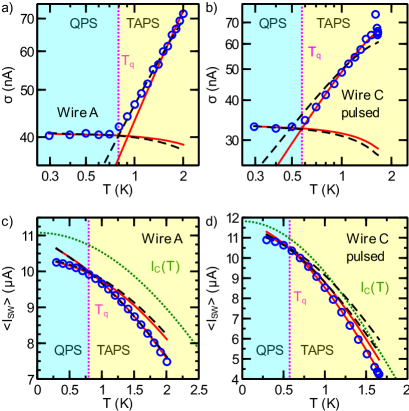
Figure 3: [Color online] (c) and (d) The average switching current and (a) and (b) its standard deviation are plotted vs temperature. The computed critical current $I_{c}(T)$ is also plotted for comparison in (c) and (d). (a) Sample A, unpulsed. (b) Sample C, pulsed. In (a) and (b) the fits are generated by Eq. (3). The two almost-horizontal curves (solid and dashed), fitting well the low-temperature part, correspond to the QPS-dominated regime. They are computed assuming $T_{esc}=T_{q}$ in Eq. (3), where $T_{q}=$0.8 K for sample A and $T_{q}=$0.6 K for sample C. The two other curves (solid and dashed), which fit well the high temperature part of the data, represent TAPS according to Eq. (3), with $T_{esc}=T$. The solid red curve corresponds to $b=5/4$, and the dashed black curve corresponds to $b=3/2$. (c) Unpulsed $\langle I_{sw}\rangle$ and (d) pulsed $\langle I_{sw}$. $T_{q}$ is indicated by the vertical dotted line. The fits to $\langle I_{sw}\rangle$ are also shown, following the convention explained in (a) and (b), according to Eq. (2). The green dotted line is $I_{c}(T)$ from Bardeen’s expression, which is used to compute $\langle I_{sw}\rangle$. Note that $\langle I_{sw}\rangle$ does not saturates at $T_{q}$ and keeps increasing for lower $T$.

We now turn to the discussion and analysis of the main results. Following the Kurkijärvi-Garg (KG) theory Kurkijarvi ; Garg-PRB95 the rate of phase slips, FD such as shown in Fig. 2(b), can be written in the general form

$$\Gamma=\Omega\exp[-u(1-I/I_{c})^{b}]\,,$$ (1)

where $I$ and $I_{c}$ are the bias and critical currents, respectively, $\Omega=\Omega_{0}(1-I/I_{c})^{a}$ is the attempt frequency, and $u=U_{c}(T)/T_{esc}$, where $U_{c}$ is a model-dependent free-energy barrier for a phase slip at $I=0$. Parameter $T_{esc}$ is known as the effective escape temperature. In the case of thermal escape, $T_{esc}=T$, according to Arrhenius law, where $T$ is the bath temperature. In the quantum fluctuation-dominated regime $T_{esc}$ is the energy of zero-point fluctuations. We have checked explicitly that this energy equals the crossover temperature $T_{q}$ (see the Appendix for details). Thus in the QPS regime $T_{esc}=T_{q}$.

Exponent $b$ defines the dependence of the phase-slip barrier on $I$. While the value of this exponent is well known for thermally activated phase slips, in the quantum regime the value of $b$ is poorly understood. Thus experimental determination of $b$ represents a significant interest to the community. The approximate linearity of the semi logarithmic plots $\Gamma(I)$ (see the Appendix for details), which is especially pronounced at low temperatures in the QPS regime [curves on the right in Fig. 2(b)], provides a useful estimate for the current exponent $b_{\textsc{qps}}\sim 1$.

As was shown in Refs. Sahu-NatPhys09, ; Li-PRL11, and Shah-PRL07, , a single phase-slip event is sufficient to drive a nanowire into the resistive state so that the temperature dependence of the dispersion is power law. In all our high-critical-current samples (unpulsed samples A–D, and also C-pulsed, and D-pulsed) the power law is observed, as is illustrated in Fig. 3 for two representative samples (see the range $T_{q}<T<$2 K).

As the temperature is lowered, the TAPS rate drops exponentially, while the QPS rate remains finite. This leads to the crossover between thermal and quantum regimes, which occurs at $T_{q}$. It will be shown below that a definite relation exists between the superconducting transition temperature $T_{c}$ and $T_{q}$. We suggest that experimental observation of such relation can be used as a tool in identifying MQT. In particular, we use this approach to eliminate the possibility of noise-induced switching and thus confirm the QPS effect.

According to the KG theory Kurkijarvi ; Garg-PRB95 , the average value of the switching current is given by

$$\langle I_{sw}\rangle\simeq I_{c}\left[1-u^{-1/b}\kappa^{1/b}\right]\,.$$ (2)

Here $\kappa=\ln(\Omega_{0}t_{\sigma})$, and $t_{\sigma}$ is the time spent sweeping through the transition. Since $\Omega_{0}t_{\sigma}$ is present only in the logarithm, its exact value is fairly unimportant. Dispersion $\sigma$ of the switching current which corresponds to the escape rate in Eq. (1) can be approximated as

$$\sigma\simeq\frac{\pi I_{c}}{\sqrt{6}b}u^{-1/b}\kappa^{(1-b)/b}=\frac{\pi I_{c}}{\sqrt{6}b\kappa}\left[1-\frac{\langle I_{sw}\rangle}{I_{c}}\right]\,.$$ (3)

Let us discuss first the higher-temperature TAPS regime. To distinguish the Josephson junction (JJ) from the phase-slip junction (PSJ), as we call our superconducting nanowire following Ref. MN-NatPhys06, , we consider in parallel two basic models. The JJs are commonly described by the McCumber-Stewart model McCumberStewart ; FD with the corresponding washboard potential. It can be solved exactly and gives $U_{c}=2\sqrt{2}\hbar I_{c}/3e$ and $b=3/2$. The PSJ barrier for the current-biased condition, Tinkham-PRB03 ; McCumberGibbsenergy which is our case, is $U_{c}=\sqrt{6}\hbar I_{c}/2e$ and the power is $b=5/4$. Although $U_{c}$ is very close in both models, it is expected that different scaling determined by $b$ will translate into different current switching dispersions.

Figures. 3(a) and 3(b) show our main results for the temperature dependence of the standard deviation for one representative unpulsed wire and one pulsed wire (see the Appendix for more information). In all the cases $\sigma(T)$ decreases as a power law and saturates to a constant value at low temperatures. The higher-temperature regime of TAPS appears in good agreement with the KG theory. All our amorphous wires show properties somewhat similar to JJs ($b_{\mathrm{TAPS}}=3/2$), indicating that the barrier for phase slips depends on the bias current as $(1-I/I_{c})^{3/2}$. The two pulsed and crystallized wires agree better with the predictions of PSJ model for perfectly homogeneous one-dimensional (1D) wires ($b_{\mathrm{TAPS}}=5/4$). The QPS phenomenon is present in both types of wires, as is evidenced by the observed saturation of the dispersion. Thus we conclude that the QPS is ubiquitous, as it occurs in amorphous wires and in 1D crystalline wires. Note that the pulsed crystalline wires are more into the 1D limit since their coherence length is larger while their diameter, measured under scanning electron microscopy (SEM), is not noticeably affected by the pulsing crystallization [see inset in Fig. 2(a)].

Now let us focus on the quantum fluctuations represented by the saturation of $\sigma$ at low temperatures $T<T_{q}$. The observed crossover is a key signature of MQT. Strong evidence that the saturation is not due to any sort of EM noise or an uncontrolled overheating of electrons above the bath temperature follows from the fact that although $\sigma$ is constant at $T<T_{q}$, the switching current keeps growing with cooling, even at $T<T_{q}$ [see Figs. 3(c) and 3(d)]. The observed saturation of $\sigma$ for $T<T_{q}$ and the simultaneous increase of $\langle I_{sw}\rangle$ with cooling at $T<T_{q}$ are in agreement with the QPS theoretical fits of the KG theory (Fig. 3). The value of the critical current here is taken from Bardeen’s formula Bardeen-RMP62 : $I_{c}=I_{c0}(1-(T/T_{c})^{2})^{3/2}$, which works well at all temperatures below $T_{c}$. Brenner-PRB11 The critical current at zero temperature $I_{c0}$ and $T_{c}$ are used as fitting parameters. Such MQT-reassuring behavior (i.e., saturation of $\sigma$ when $\langle I_{sw}\rangle$ does not show saturation) has not been observed previously on superconducting nanowires and constitutes our key evidence for QPSs.

Conventionally, the crossover temperature $T_{q}$ between regimes dominated by thermal or quantum phase slips is defined as a temperature at which the thermal activation exponent becomes equal to the quantum action, both evaluated at zero-bias current. GZTAPS ; Khlebnikov Such definition is limited to small-bias currents; thus it is not applicable to our study since it neglects the role of the bias current, which in our case is the key control parameter.Note ; Khlebnikov-ArXiv

Alternatively, the strength of a phase-slip mechanism can be described by the deviation of the average switching current from the idealized critical current of the device $I_{c}$, which is the switching current in the absence of stochastically induced phase slips. Such a characterization provides an assessment of the tunneling rate since it is the latter which determines $\langle I_{sw}\rangle$. Using $I_{c}-\langle I_{sw}\rangle$ as a measure of a phase-slip tunneling rate and accounting for the fact that the idealized critical current of the device is a phase-slip-independent quantity, we arrive at the following implicit definition of the crossover temperature $T_{q}$: $\langle I_{sw,1}(T_{q})\rangle=\langle I_{sw,2}(T_{q})\rangle$ where 1 and 2 denote two phase slip-driving mechanisms. Assuming that $\langle I_{sw,i}\rangle$ can be represented by a generic expression (2) and that parameters $\Omega_{0}$, $a$, $u$, and $b$ can be specified for a particular phase-slip mechanism, the above equation reduces to

$$u_{1}^{1/b_{1}}(T_{q})=\gamma\,u_{2}^{1/b_{2}}(T_{q}).$$ (4)

Constant $\gamma\equiv\kappa_{1}^{1/b_{1}}/\kappa_{2}^{1/b_{2}}$ depends only logarithmically on temperature and other parameters; such dependence is subleading and will be neglected.

To calculate $T_{q}$ using Eq. (4) knowledge of phase-slip parameters $u_{i}$ and $b_{i}$ is required. For a long wire in the TAPS regime these are given by $u_{\textsc{taps}}=(11.34/T)sN_{0}\sqrt{D}(T_{c}-T)^{3/2}$ and $b_{\textsc{taps}}=5/4$, where $s$ is the wire cross section, $D$ is the diffusion coefficient, and $N_{0}$ is the density of states.GZTAPS In the QPS regime $u_{\textsc{qps}}=A\,sN_{0}\sqrt{D\Delta}$ where $A$ is a numerical constants of order 1 and $\Delta$ is the temperature-dependent gap. GZTAPS ; Khlebnikov Since a posteriori $T_{q}\ll T_{c}$, one can safely approximate $\Delta$ by its zero-temperature value $\Delta=1.76T_{c}$.

The value of $b_{\textsc{qps}}$ (the exponent which governs the current dependence of the QPS action) is poorly known. Motivated by the fact that the fits to rates $\Gamma$ shown on Fig. 2(b) are made with the same value of $b$ for all temperatures and match the data well, we make a plausible assumption that $b_{\textsc{qps}}\approx b_{\textsc{taps}}$. Then, combining Eq. (4) with the expressions for $u_{\textsc{qps}}$ and $u_{\textsc{taps}}$ given above, one arrives at the conclusion that $T_{q}\propto T_{c}$. This is in agreement with our experimental finding that $T_{q}\approx 0.16T_{c}$. The observed coefficient of proportionality 0.16 implies that $\gamma^{b}A\approx 41$.

In practice, when looking for MQT/QPSs through the temperature dependence of the switching-current distribution, one has to worry about the alternative explanation that the $\sigma$ saturation is caused by the presence of a constant noise level. Such saturation, if present, can also be analyzed in the framework outlined above. Modeling noise as a thermal bath with temperature $T_{n}$ one obtains that the crossover temperature to the noise-dominated phase-slip regime is equal to $T_{n}$ and hence does not correlate with $T_{c}$, which is in contrast to our observation, [Fig. 1(a)]. We also argue that wires which are less susceptible to the noise, i.e., the wires with higher critical temperatures and therefore larger barriers for phase slips, exhibit more pronounced quantum effects; i.e., their saturation temperature $T_{q}$ is larger. We conclude therefore that the correlation between the crossover temperature and the critical temperature, observed in our experiment [Fig. 1(a)], is strong evidence in favor of MQT below $T_{q}$.

The saturation of $\sigma$ at low temperatures is seen on all tested samples, A-F [Fig. 1(c)], which have critical currents of 11.1, 12.1, 13.1, 9.23, 5.9, and 4.3 $\mu$A, respectively (see Appendix for additional data). Samples E and F have relatively low critical currents. This fact leads to the occurrence of multi-phase-slip switching events (MPSSE), manifested by the characteristic drop of $\sigma$ with increasing $T$, observed at higher temperatures. Such a drop was already observed on nanowires with relatively low critical currents (between 1.1 and 6.1 $\mu$A) in Refs. Sahu-NatPhys09, ; Li-PRL11, , which represents an important consistency check for our findings. Here we focus on samples with higher critical currents, which do not exhibit MPSSEs and do not analyze our samples E and F, which exhibit MPSSEs [Fig. 1(b)].

IV Summary

In summary, we demonstrate that in nanowires at moderately high temperatures, $T>T_{q}$, the switching into the normal state at high bias is governed by TAPSs. The corresponding standard deviation of the switching current follows the Kurkijärvi-type power-law temperature dependence $\sigma\propto T^{1/b}$. At low temperatures, $T<T_{q}$ the dispersion of the switching distribution becomes temperature independent. The crossover temperature $T_{q}$ from the TAPS- to the QPS-dominated regime is proportional the wire’s critical temperature, in agreement with theoretical arguments. Thus QPSs are unambiguously found in amorphous and single-crystal nanowires in the regime of high bias currents, i.e., near the critical current.

Acknowledgment

This material is based upon work supported by the DOE Grant No. DEFG02-07ER46453 and by the NSF Grant No. DMR 10-05645. A.-L. acknowledges support from Michigan State University.

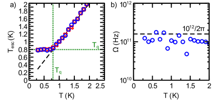
Figure 4: [Color online] (a) The fitting parameter $T_{esc}$ that defines the escape rate in Eq. (1) presented as a function of temperature. (b) Temperature dependence of the escape frequency.

V Appendix

(a) Escape temperature and attempt frequency. The fitting parameter $T_{esc}$ for wire A is shown versus temperature in Fig. 4a. For reference, the values of $T_{q}$, extracted from the mean switching current and standard deviation fits, are plotted on both horizontal and vertical scales as a dotted green lines. One can clearly identify the regime of thermally dominated escape $T_{esc}=T$ (shown by a black dashed line) above $T_{q}$ and the regime of intrinsically quantum escape with an effective temperature $T_{esc}=T_{q}$ at low temperatures.

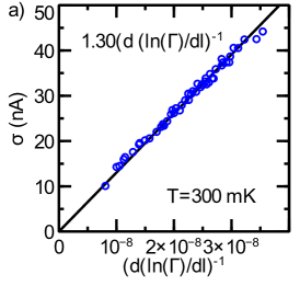
Figure 5: [Color online] Standard deviation vs inverse $d\ln\Gamma/dI$ at base temperature $T=0.3$ K, which is already deep into the quantum regime.

Having measured $\sigma(T)$, one can invert Eq. (3) to find the corresponding $T_{esc}$ and perform the consistency check for the theoretical model. The found $T_{esc}$ is plotted in Fig. 4(a) as red crosses, which also matches well with the escape temperature obtained by fitting the rates (shown as blue circles).

In Fig. 4(b) we present the temperature dependence of the attempt frequency introduced in Eq. (1). The dashed line corresponds to the characteristic frequency $2\pi\Omega=1/\sqrt{LC}\approx 10^{12}$ s^-1, where $L\approx 1$ nH and $C\approx 1$ fF are the kinetic inductance and geometrical capacitance of the wire and the electrodes correspondingly.

Figure 6: Table of fitting parameters.

(b) Relation between $\sigma$ and $d\ln\Gamma/dI$. We use experimental data for the switching rates $\Gamma(I)$ from Fig. 2b to check how the slope $d\ln\Gamma/dI$ relates to the dispersion $\sigma$. Note that this slope is defined by the slope of straight line fits in Fig.2(b) taken at the lowest temperature. The results of such an analysis are presented in Fig. 5. We find a linear dependence of the dispersion with respect to the inverse slope of the semilogarithmic plots of the switching rate versus the current. The result is in agreement with the theorem proven in Ref. Bezryadin-Review, . The best linear fit provides solid justification for the applicability of the KG model in quantum regime, which we used for the interpretation of our results.

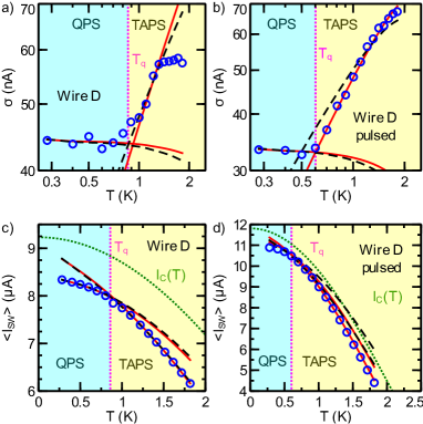
Figure 7: [Color online] Standard deviations and critical currents versus temperature for wire D before and after pulsing. The convention for lines follow that explained in the caption of Fig. 3 in the main text.

(c) Fitting parameters. Table shown in Fig. 6 summarizes all the fitting parameters used for the data analysis and interpretation. The measurements were done for eight different wires labeled from A to F. For wires C and D pulsation was applied, which is indicated in Table by a subscript (p). The value of power exponent $b$ which gave the best fit for the data is listed for every wire. Note that for all wires the critical current at zero temperature, $I_{c0}$, is slightly higher than that for the switching current $I_{cw0}$ at base temperature. The critical temperature used to fit the mean and standard deviation of the switching current, $T^{\prime}_{c}$, is relatively close to the critical temperature used to fit the resistance versus temperature data. $R(T)$ analysis was done by using result for TAPSs:

$$R(T)=R_{n}\exp[-\Delta F(T)/T],$$ (5)

where $R_{n}$ is the normal state resistance of the nanowire, and

$$\Delta F(T)=0.83\frac{R_{q}}{R_{n}}\frac{L}{\xi(0)}T_{c}[1-(T/T_{c})^{2}]^{3/2}$$ (6)

is the free-energy barrier for phase slips. Here $R_{q}=h/4e^{2}$ is the resistance quantum, $L$ is the length of the wire, and $\xi(0)$ is the zero-temperature coherence length. Equations (5) and (6) define the so-called Little’s fit. Finally, coefficient $D$ in the table was introduced for the activation energy of the PSJ model as $U_{c}=D\sqrt{6}\hbar I_{c}/2e$.

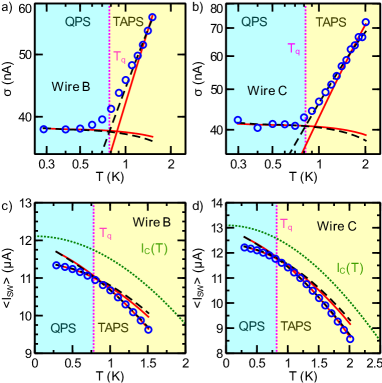
Figure 8: [Color online] Standard deviations and critical currents versus temperature for wires $B$ and $C$. The convention for lines follow that explained in the caption of Fig. 3 in the main text.

For completeness, we show in Figs. 7-8 additional experimental data for the measured standard deviations and the corresponding switching currents for the other wires listed in the table of Fig. 6. These additional samples consistently show saturation of the dispersion of the switching current at low temperatures, where quantum phase slips proliferate. What is of particular significance is that the saturation of the dispersion is accompanied by the continued increase (with cooling) of the mean switching current below the crossover temperature. The theoretical fits are in good agreement with such observed behavior.

References

- (1) W. A. Little, Phys. Rev. 156, 396 (1967).
- (2) M. Tinkham, Introduction to Superconductivity, 2nd ed. (McGraw, NY, 1996).
- (3) K. Yu. Arutyunov, D. S. Golubev, and A. D. Zaikin, Phys. Rep. 464, 1 (2008).
- (4) A. Bezryadin, J. Phys.: Condens. Matter 20, 043202 (2008); Superconductivity in nanowires: Fabrication and quantum transport, (Wiley-VCH, NY 2012).
- (5) J. M. Martinis, M. H. Devoret, and J. Clarke, Phys. Rev. B 35, 4682 (1987).
- (6) N. Giordano, Phys. Rev. Lett. 61, 2137 (1988); Phys. Rev. Lett. 63, 2417 (1989); Phys. Rev. B 41, 6350 (1990).
- (7) M. Sahu, M.-H Bae, A. Rogachev, D. Pekker, T.-C. Wei, N. Shah, P. M. Goldbart, and A. Bezryadin, Nat. Phys. 5, 503 (2009).
- (8) J. E. Mooij and Yu. V. Nazarov, Nat. Phys. 2, 169 (2006).
- (9) I. M. Pop, I. Protopopov, F. Lecocq, Z. Peng, B. Pannetier, O. Buisson, and W. Guichard, Nat. Phys. 6, 589 (2010).
- (10) J. E. Mooij and C. Harmans, New J. Phys. 7, 219 (2005).
- (11) A. M. Hriscu and Y. V. Nazarov, Phys. Rev. Lett. 106, 077004 (2011).
- (12) T. T. Hongisto, A. B. Zorin, Phys. Rev. Lett. 108, 097001 (2012).
- (13) O. V. Astafiev, L. B. Ioffe, S. Kafanov, Yu. A. Pashkin, K. Yu. Arutyunov, D. Shahar, O. Cohen, and J. S. Tsai, Nature 484, 355 (2012).
- (14) A. V. Herzog, P. Xiong, and R. C. Dynes, Phys. Rev. B 58, 14199 (1998).
- (15) A. Bezryadin, C. N. Lau, and M. Tinkham, Nature 404, 971 (2000).
- (16) A. Johansson, G. Sambandamurthy, D. Shahar, N. Jacobson, and R. Tenne, Phys. Rev. Lett. 95, 116805 (2005).
- (17) A. T. Bollinger, R. C. Dinsmore, III, A. Rogachev, and A. Bezryadin, Phys. Rev. Lett. 101, 227003 (2008).
- (18) C. N. Lau, N. Markovic, M. Bockrath, A. Bezryadin and M. Tinkham, Phys. Rev. Lett. , 87, 217003 (2001).
- (19) A. T. Bollinger, A. Rogachev, and A. Bezryadin, Europhys. Lett. 76, 505 (2006).
- (20) P. Li, P. M. Wu, Y. Bomze, I. V. Borzenets, G. Finkelstein, and A. M. Chang, Phys. Rev. Lett. 107, 137004 (2011).
- (21) N. Shah, D. Pekker, and P. M. Goldbart, Phys. Rev. Lett. 101, 207001 (2007).
- (22) J. Kurkijrvi, Phys. Rev. B 6, 832 (1972).
- (23) T. Aref and A. Bezryadin, Nanotech. 22, 395302 (2011).
- (24) M. Tinkham, J. U. Free, C. N. Lau, and N. Markovic, Phys. Rev. B 68, 134515 (2003).
- (25) D. E. McCumber, J. Appl. Phys. 39, 3113 (1968); W. C. Stewart, Appl. Phys. Lett. 12, 277 (1968).
- (26) D. E. McCumber, Phys. Rev. 172, 427 (1968).
- (27) T. A. Fulton and L. N. Dunkleberger, Phys. Rev. B 9, 4760 (1974).
- (28) A. Garg, Phys. Rev. B 51, 15592 (1995).
- (29) D. S. Golubev and A. D. Zaikin, Phys. Rev. B 78, 144502 (2008).
- (30) S. Khlebnikov, Phys. Rev. B 77, 014505 (2008); Phys. Rev. B 78, 014512 (2008).
- (31) J. Bardeen, Rev. Mod. Phys. 34, 667 (1962).
- (32) M. W. Brenner et al., Phys. Rev. B 83, 184503 (2011); Phys. Rev. B 85, 224507 (2012).
- (33) M. Tinkham and C. N. Lau, Appl. Phys. Lett. 80, 2946 (2002).
- (34) For the rate taken from Eq. (1) the analytical solution for the current switching distribution is in the form of the Gumbel distribution. The Gumbel distribution is defined by the two-parameter function .
- (35) A more appropriate definition of the crossover temperature between regimes 1 and 2 could involve corresponding phase slip-rates evaluated at a typical current which can be taken to be the average switching current (we assume “” is QPS and “” is TAPS). Such rates characterize the strength of phase-slip mechanisms. The crossover temperature is then defined by the condition . A drawback of such a definition is that it involves two, in general different, values of , while experimentally the switching always occurs at some uniquely defined .
- (36) The role of biasing current on switching was addressed in the recent work of S. Khlebnikov, arXiv:1201.5103.