Derived bracket construction up to homotopy and Schröder numbers

Abstract

On introduit la notion de la construction crochet dérivé supérieure dans la catégorie des opérades. On prouve que la construction crochet dérivé supérieure de l’opérade $\mathcal{L}ie$ est identique á la construction cobar de l’opérade $\mathcal{L}eib$ de Jean-Louis Loday. Ce théorèm est démontré par le calcul du nombre de Ernst Schröder. On trouve que la collection d’arbres racinés étiquetés peut être décomposé par l’opérade $\mathcal{L}ie$ et une nouvelle opérade.

1 Introduction

The aim of this note is to prove an identity below.
Theorem. $\mathbf{s}\mathcal{L}eib_{\infty}\cong\mathcal{L}ie\otimes\mathcal{D}_{\infty}$,
where $\mathbf{s}(-)$ is an operadic suspension, $\mathcal{L}eib$ is the operad of Leibniz (or Loday) algebras, $\mathcal{L}ie$ is the one of Lie algebras, $\mathcal{L}eib_{\infty}$ is the strong homotopy version of $\mathcal{L}eib$ and $\mathcal{D}_{\infty}=(\mathcal{D}_{\infty},\mathbf{d})$ is a new dg operad, which is called a deformation operad. Here $\mathbf{d}$ is a differential on $\mathcal{D}_{\infty}$ and the tree differential on $\mathbf{s}\mathcal{L}eib_{\infty}$ is equivalent to $\mathcal{L}ie\otimes\mathbf{d}$. Remark that $\mathcal{D}_{\infty}$ is not strong homotopy operad in usual sense. The following identity is already known,

$$\mathbf{s}\mathcal{L}eib\cong\mathcal{L}ie\otimes\mathbf{s}\mathcal{P}erm,$$

where $\mathcal{P}erm$ is Chapoton’s permutation operad [4]. Theorem is regarded as a homotopy version of this classical identity.
The dg operad $\mathcal{D}_{\infty}$ is defined as a deformation of $\mathbf{s}\mathcal{P}erm$. The operad $\mathbf{s}\mathcal{P}erm$ can be constructed with a formal differential $d_{0}$ and the commutative associative operad $\mathcal{C}om$. The deformation operad will be constructed by using a deformation differential, $\hbar d_{1}+\hbar^{2}d_{2}+\cdots$, instead of $d_{0}$. As a corollary of Theorem we prove that $(\mathcal{D}_{\infty},\mathbf{d})$ is a resolution over $\mathbf{s}\mathcal{P}erm$.
To prove Theorem we compute (small-)Schröder numbers (See Table 1.)

$n$	1	2	3	4	5	6	7	8	9	10
$s(n)$	1	1	3	11	45	197	903	4279	20793	103049

Table 1: Schröder numbers

The Schröder number $s(n)$ is known as the cardinal number of planar rooted trees with $n$-leaves, on the other hand, $\mathbf{s}\mathcal{L}eib_{\infty}$ is, as an operad, isomorphic to the operad of labeled planar rooted trees. Theorem says that the set of labeled planar rooted trees is decomposed into $\mathcal{L}ie$ and $\mathcal{D}_{\infty}$. This gives a new interpritation of Schröder numbers.
The generator of $\mathcal{L}ie\otimes\mathcal{D}_{\infty}$ has the following form,

$$\{\{\{\{d_{n-1}(1),2\},3\},...,n\}.$$

Here $\{,\}$ is a Lie bracket in $\mathcal{L}ie(2)$ and $d_{n}$ is a formal derivation. The bracket of this type is called a higher derived bracket or derived bracket up to homotopy. In particular, when $n=2$, $\{d_{1}(1),2\}$ is called a binary derived bracket. The notion of (binary) derived bracket was defined by Kosmann-Schwarzbach [7] in the study of Poisson geometry (see also [8].) The higher version was introduced by several authors (cf. Roytenberg [13], Voronov [18].) Derived brackets were born in Poisson geometry, however, an important development of derived bracket theory was made in the study of algebraic operads by Aguiar [1]. Aguiar discovered that several types of algebras are induced by the method of derived bracket construction. Inspired by Aguiar’s work, Uchino [16] introduced the notion of binary derived bracket construction on the level of operad. This is an endofunctor on the category of binary quadratic operads defined by applying the permutation operad, $(-)\otimes\mathbf{s}\mathcal{P}erm:\mathcal{P}\mapsto\mathcal{P}\otimes\mathbf{s}\mathcal{P}erm$. In non graded case, $(-)\otimes\mathcal{P}erm$. The derived bracket on the level of algebra is regarded as a representation of this functor.
In this article, we will try to make a higher version of $(-)\otimes\mathbf{s}\mathcal{P}erm$. Our solution is not $(-)\otimes\mathbf{s}\mathcal{P}erm_{\infty}$, but the functor $(-)\otimes\mathcal{D}_{\infty}$ appeared in Theorem above. We call this functor a higher derived bracket construction (on the level of operad.) The strong homotopy Leibniz operad $\mathbf{s}\mathcal{L}eib_{\infty}$ is the result of cobar construction with Koszul duality theory (Ginzburg and Kapranov [5].) Hence the theorem means that the higher derived bracket construction of $\mathcal{L}ie$ coincides with the cobar construction of $\mathcal{L}eib$. An advantage of the higher derived bracket construction is that it uses no Koszul duality theory.

2 Preliminaries

2.1 Assumptions and Notations

Through the paper, all algebraic objects are assumed to be defined over a fixed field $\mathbb{K}$ of characteristic zero. The mathematics of graded linear algebra is due to Koszul sign convention. Namely, the transposition of tensor product satisfies $o_{1}\otimes o_{2}\cong(-1)^{|o_{1}||o_{2}|}o_{2}\otimes o_{1}$ for any objects $o_{1}$ and $o_{2}$, where $|o_{i}|$ is the degree of $o_{i}$. We denote by $s(-)$ a suspension of degree $+1$. For any object $o$, the degree of $s(o)$ is $|s(o)|=|o|+1$. The inverse of $s$ is $s^{-1}$, whose degree is $-1$.

2.2 Algebraic operads

We refer the readers to Loday [9, 10, 11] and Loday-Vallette [12], for the details of algebraic operad theory.
An $\mathcal{S}$-module, $\mathcal{P}:=(\mathcal{P}(1),\mathcal{P}(2),...)$, is by definition a collection of $S_{n}$-modules $\mathcal{P}(n)$, where $S_{n}$ is the $n$th symmetric group. The notion of morphism between $\mathcal{S}$-modules is defined by the usual manner, i.e., it is a collection $\phi=(\phi(1),\phi(2),...)$ of equivariant linear mappings $\phi(n):\mathcal{P}_{1}(n)\to\mathcal{P}_{2}(n)$. Here $\mathcal{P}_{1}$ and $\mathcal{P}_{2}$ are any $\mathcal{S}$-modules. Thus the category of $\mathcal{S}$-modules is defined.
In the category of $\mathcal{S}$-modules, a tensor product, $\mathcal{P}_{1}\odot\mathcal{P}_{2}$, is defined by

$$(\mathcal{P}_{1}\odot\mathcal{P}_{2})(n):=\bigoplus_{m,l}\mathcal{P}_{1}(m)\otimes_{S_{m}}\Big{(}\mathcal{P}_{2}(l_{1}),...,\mathcal{P}_{2}(l_{m})\Big{)}\otimes_{(S_{l_{1}},...,S_{l_{m}})}S_{n},$$

where $n=l_{1}+\cdots+l_{m}$ and $l:=(l_{1},...,l_{m})$. It is easy to see that the tensor product is associative. We consider a special $\mathcal{S}$-module $\mathcal{I}:=(\mathbb{K},0,0,...)$. It is easy to check that $\mathcal{I}\odot\mathcal{P}\cong\mathcal{P}\cong\mathcal{P}\odot\mathcal{I}$. The concept of binary product on $\mathcal{P}$ is defined as a morphism of $\gamma:\mathcal{P}\odot\mathcal{P}\to\mathcal{P}$.

Definition 2.1 (algebraic operad).

A triple $\mathcal{P}:=(\mathcal{P},\mathcal{I},\gamma)$ is called an algebraic operad, or shortly operad, if it is a unital monoid in the category of $\mathcal{S}$-modules.

If $\mathcal{P}$ is an operad, $\mathcal{P}(n)$ is considered to be a space of formal $n$-ary operations. For example $\mathcal{P}(2)$ is a space of formal binary operations, which are usually denoted by $1*2$, $1\cdot 2$, $[1,2]$, $\{1,2\}$ and so on. The operad structure $\gamma$ defines a composition product on the operations, for instance,

$$\gamma:\{1,2\}\otimes([1,2],1*2)\mapsto\{[1,2],3*4\},$$

$$\gamma:[2,1]\otimes(1_{\mathcal{P}},\{1,2\})\mapsto[\{2,3\},1],$$

where $1_{\mathcal{P}}$ is the unite element of $\mathcal{P}$. The numbers $1,2,3,...$ in the formal products are called labels or leaves.

Definition 2.2.

For any $p_{m}\in\mathcal{P}(m)$, $p_{n}\in\mathcal{P}(n)$,

$$p_{m}\circ_{i}p_{n}:=\gamma\Big{(}p_{m}\otimes\big{(}1_{\mathcal{P}}^{\otimes(i-1)}\ ,\ p_{n}\ ,\ 1_{\mathcal{P}}^{\otimes(m-i)}\big{)}\Big{)}.$$

where $1\leq i\leq m$.

The composition $p_{m}\circ_{i}p_{n}$ values in $\mathcal{P}(m+n-1)$. The structure $\gamma$ is decomposed into the compositions $(\circ_{1},\circ_{2},...)$.

Definition 2.3 (free operad).

Let $\mathcal{P}$ be an $\mathcal{S}$-module not necessarily operad. The free operad over $\mathcal{P}$, which is denoted by $\mathcal{T}\mathcal{P}$, is by definition the free unital monoid in the category of $\mathcal{S}$-modules.

It is easy to see that $(\mathcal{T}\mathcal{P})(1)\cong T\mathcal{P}(1)$ the tensor algebra over $\mathcal{P}(1)$. We denote the quadratic part of $\mathcal{T}\mathcal{P}$ by $\mathcal{T}^{2}\mathcal{P}$,

$$(\mathcal{T}^{2}\mathcal{P})(m+n-1)=<p_{m}\circ_{i}p_{n}\ |\ 1\leq{i}\leq m>,$$

in particular, $(\mathcal{T}^{2}\mathcal{P})(1)=\mathcal{P}(1)\circ_{1}\mathcal{P}(1)\cong\mathcal{P}(1)\otimes\mathcal{P}(1)$.

Definition 2.4 (quadratic operad).

Let $R\subset\mathcal{T}^{2}\mathcal{P}$ be a sub $\mathcal{S}$-module of $\mathcal{T}\mathcal{P}$. The quotient operad $\mathcal{O}:=\mathcal{T}^{2}\mathcal{P}/(R)$ is called a quadratic operad, where $(R)$ is an ideal generated by $R$. The generator $R$ is called a quadratic relation. If $\mathcal{P}=\mathcal{P}(2)$ with $\mathcal{P}(n\neq 2)=0$, $\mathcal{O}$ is called a binary quadratic operad.

We recall two examples of binary quadratic operads. The Lie operad, $\mathcal{L}ie$, is a binary quadratic operad generated by a formal skewsymmetry bracket $\{1,2\}(=-\{2,1\})$.

$$\mathcal{L}ie:=\mathcal{T}(\{1,2\})/(R_{\mathcal{L}ie}).$$

The quadratic relation $R_{\mathcal{L}ie}$ is generated by the Jacobi identity,

$$\{\{1,2\},3\}+\{\{3,1\},2\}+\{\{2,3\},1\}=0.$$

We obtain the following expression of $\mathcal{L}ie$.

$$\mathcal{L}ie(1) = \mathbb{K},$$

$$\mathcal{L}ie(2) = <\{1,2\}>,$$

$$\mathcal{L}ie(3) = <\{\{1,2\},3\}\ ,\ \{\{1,3\},2\}>,$$

$$\cdots \cdots \cdots.$$

Lemma 2.5.

$\dim\mathcal{L}ie(n)=(n-1)!$.

Proof.

An arbitrary bracket in $\mathcal{L}ie(n)$ is generated by the right-normed brackets

$$\{\sigma(1),\{\sigma(2),...,\{\sigma(n-1),n\}\}\},$$

where $\sigma\in S_{n-1}$. ∎

The commutative associative operad, $\mathcal{C}om$, is generated by a formal commutative product. We denote by $1\otimes 1$ the commutative product.

$$\mathcal{C}om:=\mathcal{T}(1\otimes 1)/(R_{\mathcal{C}om}).$$

The quadratic relation $R_{\mathcal{C}om}$ is the associative law,

$$(1\otimes 1)\otimes 1-1\otimes(1\otimes 1)=0.$$

We obtain the following expression of $\mathcal{C}om$.

$$\mathcal{C}om(1) = \mathbb{K},$$

$$\mathcal{C}om(2) = <1\otimes 1>,$$

$$\mathcal{C}om(3) = <1\otimes 1\otimes 1>,$$

$$\cdots \cdots \cdots.$$

It is obvious that $\mathcal{C}om(n)\cong\mathbb{K}$ for each $n$.
In the final of this subsection, we recall some basic concepts in algebraic operad theory.

Definition 2.6 (operadic suspension).

If $\mathcal{P}=(\mathcal{P}(n))$ is an operad, the shifted operad $\mathbf{s}\mathcal{P}$ is defined by

$$(\mathbf{s}\mathcal{P})(n)\cong s^{-1}\otimes\mathcal{P}(n)\otimes s^{\otimes n}\cong s^{n-1}\mathcal{P}(n)\otimes\mathrm{sgn}_{n},$$

where $\mathrm{sgn}_{n}$ is the sign representation of $S_{n}$. The inverse of $\mathbf{s}$, $\mathbf{s}^{-1}$, is defined by the same manner.

Definition 2.7 (dg operad).

By definition, a differential graded operad, or shortly dg operad, is an operad such that for each $n$ $(\mathcal{P}(n),d)$ is a complex and the differential is compatible with the operad structure, i.e., it is equivariant and satisfies the usual condition,

$$d(p_{m}\circ_{i}p_{n})=dp_{m}\circ_{i}p_{n}+(-1)^{|p_{m}|}p_{m}\circ_{i}dp_{n},$$

where $p_{m}\in\mathcal{P}(m)$ and $p_{n}\in\mathcal{P}(n)$.

Definition 2.8 (Koszul dual operad).

Let $\mathcal{P}=\mathcal{T}(E)/(R)$ be a binary quadratic operad with $\mathcal{P}(2)=E$. We put $E^{\vee}:=E^{*}\otimes\mathrm{sgn}_{2}$. The Koszul dual of $\mathcal{P}$ is by definition

$$\mathcal{P}^{!}:=\mathcal{T}(E^{\vee})/(R^{\bot}),$$

where $R^{\bot}$ is the orthogonal space of $R$.

It is obvious that $\mathcal{P}^{!!}\cong\mathcal{P}$. It is well-known that $\mathcal{L}ie^{!}\cong\mathcal{C}om$.

2.3 (Sh) Leibniz operad

We recall the notion of (sh) Leibniz algebras.

Definition 2.9 (Leibniz/Loday algebras [9, 11]).

A Leibniz algebra or Loday algebra $(L,[,])$ is by definition a vector space equipped with a binary bracket product $[,]$ satisfying the Leibniz identity,

$$[x_{1},[x_{2},x_{3}]]=[[x_{1},x_{2}],x_{3}]+[x_{2},[x_{1},x_{3}]],$$

where $x_{\cdot}\in L$.

The operad of Leibniz algebras is denoted by $\mathcal{L}eib$, which is a binary quadratic operad generated by $[1,2]$ and $[2,1]$,

$$\mathcal{L}eib:=\mathcal{T}([1,2],[2,1])/(R_{\mathcal{L}eib}),$$

where $R_{\mathcal{L}eib}$ is the Leibniz identity. If the degree of $[1,2]$ is odd, i.e., $[1,2]\in\mathbf{s}\mathcal{L}eib(2)$, then the Leibniz identity has the following form,

$$[1,[2,3]]=-[[1,2],3]-[2,[1,3]],$$

which is called an odd Leibniz identity.
We recall sh Leibniz algebras (cf. Ammar and Poncin [2]) and its operad.

Definition 2.10 (Koszul dual of Leibniz algebra [11], Zinbiel [19]).

A Zinbiel algebra $(Z,*)$ is by definition a vector space equipped with a binary product $*$ satisfying

$$x_{1}*(x_{2}*x_{3})=(x_{1}*x_{2})*x_{3}+(x_{2}*x_{1})*x_{3},$$

which is called a Zinbiel identity or dual Leibniz identity.

The operad of Zinbiel algebras is denoted by $\mathcal{Z}inb$, which is the Koszul dual of $\mathcal{L}eib$, that is, $\mathcal{Z}inb=\mathcal{L}eib^{!}$. It is known that $\mathcal{Z}inb(n)\cong S_{n}$ for each $n$ ([11]).

Lemma 2.11 ([2]).

The cofree Zinbiel coalgebra over a space $V$ is the tensor space

$$\bar{T}^{c}V:=V\oplus V^{\otimes 2}\oplus\cdots$$

equipped with the coproduct defined by

$$\Delta(x_{1},...,x_{n+1}):=\sum_{i=1}^{n}\sum_{\sigma}\epsilon(\sigma)(x_{\sigma(1)},...,x_{\sigma(i)})\otimes(x_{\sigma(i+1)},...,x_{\sigma(n)},x_{n+1}),$$

where $\epsilon(\sigma)$ is a Koszul sign and $\sigma$s are $(i,n-i)$-unshuffles permutations, that is, $\sigma(1)<\cdots<\sigma(i)$ and $\sigma(i+1)<\cdots<\sigma(n)$.

Let $\mathrm{Coder}(\bar{T}^{c}V)$ be the space of coderivations on the coalgebra.

Definition 2.12 ([2]).

Let $\partial\in\mathrm{Coder}(\bar{T}^{c}V)$ be a coderivation of degree $+1$ on the coalgebra. The pair $(V,\partial)$ is called an sh Leibniz algebra or sh Loday algebra, if $\partial^{2}=0$, that is, codifferential.

In general, the structure of sh Leibniz algebra $\partial$ has the form of deformation,

$$\partial=\partial_{1}+\partial_{2}+\cdots.$$

For each $j$, the coderivation $\partial_{j}$ is on $V^{\otimes j}$ identified to a linear map of $\partial_{j}:V^{\otimes j}\to V$, and on $V^{\otimes n\geq j}$ it satisfies

$$\partial_{j}(x_{1},...,x_{n})=\sum_{k=j}^{n}\sum_{\sigma}(\pm)(x_{\sigma(1)},...,x_{\sigma(k-j)},\partial_{j}(x_{\sigma(k-j+1)},...,x_{\sigma(k-1)},x_{k}),x_{k+1},...,x_{n}),$$

where $(\pm)$ is an appropriate sign and $\sigma$ are $(k-j,j-1)$-unshuffle permutations. The defining condition of sh Leibniz algebras, $\partial^{2}=0$, is equivalent to

$$[\partial_{1},\partial_{n}]+\sum_{i+j-1=n}\partial_{i}\partial_{j}=0.$$

There is an easy method of making sh Leibniz algebras (so-called higher derived bracket construction on the level of algebra.)

Proposition 2.13 ([17]).

Let $(\mathfrak{g},\{,\},d_{0})$ be a dg Lie algebra with a differential $d_{0}$. There exists a Lie algebra homomorphism

$$N:\mathrm{Der}(\mathfrak{g})[[\hbar]]\to\mathrm{Coder}(\bar{T}^{c}\mathfrak{g}),$$

where $\mathrm{Der}(\mathfrak{g})$ is the space of derivations on $\mathfrak{g}$. Suppose that $d_{\hbar}:=d_{0}+\hbar d_{1}+\hbar^{2}d_{2}+\cdots$ is a deformation differential of $d_{0}$. We define $\partial_{n+1}:=N(\hbar^{n}d_{n})$ for each $n$. Then $\partial=\partial_{1}+\partial_{2}+\cdots$ becomes an sh Leibniz algebra structure.

Proof.

(Sketch) The map of the proposition is defined as the higher derived bracket,

$$N(\hbar^{n}D)(x_{1},x_{2},...,x_{n+1}):=\{\{\{Dx_{1},x_{2}\},...\},x_{n+1}\},$$

for any $\hbar^{n}D\in\mathrm{Der}(\mathfrak{g})[[\hbar]]$. ∎

But now to our next task. We consider an $\mathcal{S}$-module $s\overline{\mathcal{Z}inb^{*}}:=(s\mathcal{Z}inb^{*}(n))$ with $n\geq 2$, where $\mathcal{Z}inb^{*}(n)$ is the dual space of $\mathcal{Z}inb(n)$. We denote by $T_{n}:=T_{n}(1,2,...,n)$ the generator of $s\mathcal{Z}inb^{*}(n)$. Let $\mathcal{T}(s\overline{\mathcal{Z}inb^{*}})$ be the free operad over the $\mathcal{S}$-module. This operad is generated from $(T_{n})$. One can define a differential, $d_{t}$, on the free operad by

$$d_{t}T_{2} := 0,$$ (1)

$$d_{t}T_{n}+\sum_{i+j-1=n}T_{i}T_{j} := 0,$$ (2)

where

$$T_{i}T_{j}:=\sum_{k=j}^{n}\sum_{\sigma}(T_{i}\circ_{k-j+1}T_{j})(\sigma(1),...,\sigma(k-j),\sigma(k-j+1),...,\sigma(k-1),k,k+1,...,n),$$ (3)

where $k$, $\sigma$ are the same as above. It is easy to check $d_{t}d_{t}=0$. This differential is called a tree differential.

Definition 2.14 (sh Leibniz operad).

$\mathbf{s}\mathcal{L}eib_{\infty}:=\Big{(}\mathcal{T}(s\overline{\mathcal{Z}inb^{*}}),d_{t}\Big{)}$.

Hence $\mathcal{L}eib_{\infty}=\mathbf{s}^{-1}\mathcal{T}(s\overline{\mathcal{Z}inb^{*}})$.
In the final of this section, we recall the concept of tree. A planar rooted tree with $n$-leaves is by definition a directed graph with $n$-leaves (input edges), $1$-root (output edge) and without loop (See Fig 1). A labeled planar rooted tree is a planar rooted tree whose leaves are labeled by natural numbers.

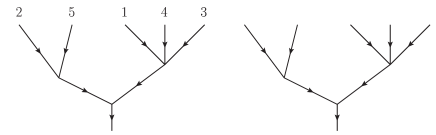
Figure 1: labeled $5$-tree and non-labeled one

Lemma 2.15.

As an operad, up to degree, $\mathbf{s}\mathcal{L}eib_{\infty}$ is isomorphic to the labeled planar rooted trees, i.e., $\mathbf{s}\mathcal{L}eib_{\infty}(n)$ is linearly isomorphic to the space of labeled planar rooted trees with $n$-leaves.

Proof.

Since $\mathcal{Z}inb(n)\cong S_{n}$, the generator $T_{n}\in s\mathcal{Z}inb^{*}(n)$ is identified to a labeled planar rooted tree with $n$-leaves and with $1$-internal vertex (See Fig 2.)

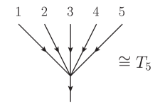
Figure 2: $T_{5}$

∎

The lemmas above will be used in Section 4.

3 Deformation operad

3.1 Permutation algebras and the operad $\mathcal{P}erm$

A permutation algebra introduced by Chapoton [4] is by definition an associative algebra $(A,*)$ satisfying

$$(a_{1}*a_{2})*a_{3}=a_{1}*(a_{2}*a_{3})=(a_{2}*a_{1})*a_{3}.$$

The operad of permutation algebras is denoted by $\mathcal{P}erm$, which is also a binary quadratic operad

$$\mathcal{P}erm:=\mathcal{T}(1*2,2*1)/(R_{\mathcal{P}erm}).$$

We recall a construction of $\mathcal{P}erm$ with a formal differential ([16]). Let $d_{0}$ be a 1-ary operator of degree $+1$ and let $1\otimes 1\in\mathcal{C}om(2)$ be a binary commutative product of degree $0$. Let $\mathcal{T}(d_{0},1\otimes 1)$ be the free operad over $(d_{0},1\otimes 1)$. We define a quadratic operad $\mathcal{Q}$,

$$\mathcal{Q}:=\mathcal{T}(d_{0},1\otimes 1)/(R_{\mathcal{Q}}),$$

where $R_{\mathcal{Q}}$ is the space of three quadratic relations,

$$(1\otimes 1)\otimes 1 = 1\otimes(1\otimes 1),$$

$$d_{0}(1\otimes 1) = d_{0}\otimes 1+1\otimes d_{0},$$

$$d_{0}d_{0} = 0.$$

The operad $\mathcal{Q}$ is a graded operad, $\mathcal{Q}=(\mathcal{Q}^{i})$, whose degree is defined as the number of $d_{0}$. In [16], it was proved that the operad $\mathbf{s}\mathcal{P}erm$ is isomorphic to the suboperad of $\mathcal{Q}$ whose $n$th component is $\mathcal{Q}^{n-1}(n)$, that is,

Lemma 3.1.

$\mathbf{s}\mathcal{P}erm\cong(\mathcal{Q}^{n-1}(n))$.

Proof.

(Sketch) We check that $(\mathcal{Q}^{n-1}(n))$ satisfies the relation of $\mathbf{s}\mathcal{P}erm$. The odd version of associative law is

$$(d_{0}\otimes 1)\circ_{1}(d_{0}\otimes 1)=-(d_{0}\otimes d_{0}\otimes 1)=-(d_{0}\otimes 1)\circ_{2}(d_{0}\otimes 1)$$

and the odd premutation relation is

$$(d_{0}\otimes 1)\circ_{1}(d_{0}\otimes 1)=-(d_{0}\otimes d_{0}\otimes 1)=-(d_{0}\otimes 1)\circ_{1}(1\otimes d_{0}).$$

∎

From this, we obtain the following expression of $\mathbf{s}\mathcal{P}erm$,

$$\mathbf{s}\mathcal{P}erm(1) = \mathbb{K},$$

$$\mathbf{s}\mathcal{P}erm(2) = <d_{0}\otimes 1\ ,\ 1\otimes d_{0}>,$$

$$\mathbf{s}\mathcal{P}erm(3) = <d_{0}\otimes d_{0}\otimes 1\ ,\ d_{0}\otimes 1\otimes d_{0}\ ,\ 1\otimes d_{0}\otimes d_{0}>,$$

$$\cdots \cdots \cdots.$$

The proposition below is the binary model of the main theorem of this note.

Proposition 3.2 (Chapoton [4] see also Vallette [15]).

$\mathbf{s}\mathcal{L}eib\cong\mathcal{L}ie\otimes\mathbf{s}\mathcal{P}erm$.

We prove this proposition by using the method of derived bracket construction.

Proof.

The elements of $\mathcal{L}ie\otimes\mathbf{s}\mathcal{P}erm$ are regarded as derived brackets, for example,

$$\{d_{0}(1),2\} \cong \{1,2\}\otimes(d_{0}\otimes 1),$$

$$\{1,d_{0}(2)\} \cong \{1,2\}\otimes(1\otimes d_{0}),$$

$$\{\{d_{0}(1),d_{0}(2)\},3\} \cong \{\{1,2\},3\}\otimes(d_{0}\otimes d_{0}\otimes 1).$$

The derivation of the bracket $d_{0}\{1,2\}$ is well-defined as a linear combination of the derived brackets,

$$d_{0}\{1,2\}:=\{d_{0}(1),2\}+\{1,d_{0}(2)\}.$$

It is easy to see that $\mathbf{s}\mathcal{L}eib(2)\cong(\mathcal{L}ie\otimes\mathbf{s}\mathcal{P}erm)(2)$ and that $\mathcal{L}ie\otimes\mathbf{s}\mathcal{P}erm$ is generated by $(\mathcal{L}ie\otimes\mathbf{s}\mathcal{P}erm)(2)$. The derived bracket satisfies the odd Leibniz identity,

$$\{d_{0}(1),\{d_{0}(2),3\}\} = \{\{d_{0}(1),d_{0}(2)\},3\}-\{d_{0}(2),\{d_{0}(1),3\}\}$$

$$= -\{d_{0}\{d_{0}(1),2\},3\}-\{d_{0}(2),\{d_{0}(1),3\}\}.$$

Hence there exists an operadic surjection $\psi:\mathbf{s}\mathcal{L}eib\to\mathcal{L}ie\otimes\mathbf{s}\mathcal{P}erm$.

$$\begin{CD}\mathcal{T}(\mathbf{s}\mathcal{L}eib(2))@=\mathcal{T}\big{(}(\mathcal{L}ie\otimes\mathbf{s}\mathcal{P}erm)(2)\big{)}\\ @V{}V{}V@V{}V{}V\\ \mathbf{s}\mathcal{L}eib@>{\psi}>{}>\mathcal{L}ie\otimes\mathbf{s}\mathcal{P}erm.\end{CD}$$

By a dimension counting, one can prove that this map is isomorphism. Since $\mathbf{s}\mathcal{P}erm(n)\cong\mathcal{Q}^{n-1}(n)$, $\dim\mathbf{s}\mathcal{P}erm(n)=n$. It is well-known that $\dim\mathcal{L}ie(n)=(n-1)!$ and $\dim\mathcal{L}eib(n)=n!$. Hence $\dim\mathbf{s}\mathcal{L}eib(n)=\dim(\mathcal{L}ie\otimes\mathbf{s}\mathcal{P}erm)(n)$ for each $n$. ∎

3.2 Deformation of $\mathcal{P}erm$

Let $V:=<d_{1},d_{2},...>$ be a space of 1-ary operators of degree $+1$ and let $1\otimes 1\in\mathcal{C}om(2)$ the same as above. Define a quadratic operad,

$$\mathcal{O}:=\mathcal{T}(V,1\otimes 1)/(R_{\mathcal{O}}),$$

where $R_{\mathcal{O}}$ is the space of quadratic relations,

$$(1\otimes 1)\otimes 1 = 1\otimes(1\otimes 1),$$

$$d_{n}(1\otimes 1) = d_{n}\otimes 1+1\otimes d_{n},\ \ \forall n\in\mathbb{N}.$$

We should remark that $\mathcal{O}(1)$ is the same as the tensor algebra over $V$,

$$\mathcal{O}(1)=\mathbb{K}\oplus V\oplus{V}^{\otimes 2}\oplus{V}^{\otimes 3}\oplus\cdots.$$ (4)

We define on the operad $\mathcal{O}$ the second degree which is called a weight. The weight function is denoted by $w(-)$.

Definition 3.3 (weight on $\mathcal{O}$).

$w(d_{n}):=n$ and $w(1^{\otimes n}):=1-n$ for each $n$.

Then $\mathcal{O}$ becomes a graded and weighted operad $\mathcal{O}=(\mathcal{O}^{g,w})$. The degree and the weight are both additive with respect to the operad structure of $\mathcal{O}$. Hence the sub $\mathcal{S}$-module of weight $0$, $(\mathcal{O}^{\bullet,0})$, becomes a suboperad of $\mathcal{O}$. We introduce the main object of this note :

Definition 3.4 (deformation operad).

$\mathcal{D}_{\infty}:=(\mathcal{O}^{\bullet,0})$.

For each $n\in\mathbb{N}$,

$$\mathcal{D}_{\infty}(n)=\mathcal{O}^{1,0}(n)\oplus\mathcal{O}^{2,0}(n)\oplus\cdots\oplus\mathcal{O}^{n-1,0}(n).$$

The elementary parts of $\mathcal{D}_{\infty}$ have the following form,

$$\mathcal{D}_{\infty}(1) = \mathbb{K}.$$

$$\mathcal{D}_{\infty}(2) = <d_{1}\otimes 1\ ,\ 1\otimes d_{1}>.$$

$$\mathcal{D}_{\infty}^{1}(3) = <d_{2}\otimes 1\otimes 1\ ,\ 1\otimes d_{2}\otimes 1\ ,\ 1\otimes 1\otimes d_{2}>.$$

$$\mathcal{D}_{\infty}^{2}(3) = <d_{1}\otimes d_{1}\otimes 1\ ,\ d_{1}\otimes 1\otimes d_{1}\ ,\ 1\otimes d_{1}\otimes d_{1}\ ,\$$

$$\ \ \ \ \ d_{1}^{2}\otimes 1\otimes 1\ ,\ 1\otimes d_{1}^{2}\otimes 1\ ,\ 1\otimes 1\otimes d_{1}^{2}>.$$

$$\cdots \cdots \cdots.$$

It is obvious that $\mathcal{D}^{1}_{\infty}(n)\cong s\mathbb{K}^{n}$ for each $n$.
One can easily prove that

Proposition 3.5.

The deformation operad is generated by $\mathcal{D}_{\infty}^{1}$.

Proof.

(Sketch) We call a monomial of derivations $d_{i_{1}}d_{i_{2}}\cdots d_{i_{f}}$ a higher order derivation of order $f$. A homogeneous element $X:=x_{1}\otimes\cdots\otimes x_{n}\in\mathcal{D}_{\infty}^{a}(n)$ is called a higher derived product of order $a$, if the derivations in $X$ are all the same position (e.g. $1\otimes d_{1}d_{2}\otimes 1\otimes 1$.) Generators of $\mathcal{D}^{1}_{\infty}$ are special higher derived products of order $1$. It is easy to prove that the deformation operad is generated by higher derived products. Hence the problem is reduced to proving that the higher derived product of any order is generated by $\mathcal{D}^{1}_{\infty}$. This will be solved by using induction w.r.t. degree. ∎

Let us define on the deformation operad a differential. If the derivations $d_{1},d_{2},...$ are deformations of a formal derivation $d_{0}$ (not necessarily differential), then the deformation derivation $d_{\hbar}:=d_{0}+\hbar d_{1}+\hbar^{2}d_{2}+\cdots$ satisfies $d_{\hbar}d_{\hbar}=d_{0}d_{0}(\neq 0)$, or equivalently,

$$[d_{0},d_{n}]+\sum_{i+j=n}d_{i}d_{j}=0,$$ (5)

where $[d_{0},d_{n}]$ is the graded commutator and $i,j,n\geq 1$. By using (5) one can define a differential on $\mathcal{D}_{\infty}$.

Definition 3.6 (differential on $\mathcal{D}_{\infty}$).

For any $x_{1}\otimes\cdots\otimes x_{n}\in\mathcal{D}_{\infty}(n)$,

$$\mathbf{d}(x_{1}\otimes\cdots\otimes x_{n}) := \sum_{i=1}^{n}(-1)^{|x_{1}|+\cdots+|x_{i-1}|}(x_{1}\otimes\cdots\otimes\mathbf{d}x_{i}\otimes\cdots x_{n}),$$

$$\mathbf{d}(x_{i}) := [d_{0},x_{i}].$$

The homogeneous condition $\mathbf{d}\mathbf{d}=0$ is followed from the Bianchi identity. Therefore, $(\mathcal{D}_{\infty},\mathbf{d})$ becomes a dg operad. For example,

$$\mathbf{d}(d_{2}\otimes 1\otimes 1) = -d_{1}^{2}\otimes 1\otimes 1$$

$$= -(d_{1}\otimes 1)\circ_{1}(d_{1}\otimes 1)-(d_{1}\otimes 1)\circ_{2}(d_{1}\otimes 1),$$

which yields

Lemma 3.7.

$\mathrm{H}^{top}(\mathcal{D}_{\infty},\mathbf{d})\cong\mathbf{s}\mathcal{P}erm$.

Remark 3.8.

$\mathcal{D}_{\infty}\neq\mathbf{s}\mathcal{P}erm_{\infty}$.

3.3 Dimension of $\mathcal{D}_{\infty}$

In this section we compute the dimension of the deformation operad. Consider a set of derivations, $A=\{d_{1}^{(\lambda_{1})}\ ,\ d_{2}^{(\lambda_{2})}\ ,\ ...\ ,\ d_{n-1}^{(\lambda_{n-1})}\}$, where $d_{i}^{(\lambda_{i})}$ is the $\lambda_{i}$-copies of $d_{i}$ (e.g. $d_{i}^{(3)}=\{d_{i},d_{i},d_{i}\}$ and $d_{i}^{(0)}:=\emptyset$.) We define a space $\Delta^{(\lambda_{1},\lambda_{2},...,\lambda_{n-1})}(n)$ as a subspace of $\mathcal{D}_{\infty}^{a}(n)$ such that each of elements has all derivations in $A$. Here the degree $a$ is equal to the cardinal number of $A$. For example, when $n=5$ and $a=2$,

$$\Delta^{(0,2,0,0)}(5) = <d_{2}d_{2}\otimes 1\otimes 1\otimes 1\ ,\ d_{2}\otimes d_{2}\otimes 1\otimes 1\ ,\ ...>,$$

$$\Delta^{(1,0,1,0)}(5) = <d_{1}d_{3}\otimes 1\otimes 1\otimes 1\ ,\ d_{1}\otimes d_{3}\otimes 1\otimes 1\ ,\ ...>,$$

which are subspaces of $\mathcal{D}^{2}_{\infty}(5)$. In particular, the top degree part of $\mathcal{D}_{\infty}(n)$ is

$$\mathcal{D}^{top}_{\infty}(n)=\mathcal{D}^{n-1}_{\infty}(n)=\Delta^{(n-1,0,...,0)}(n).$$

From the assumptions of degree and weight, we obtain two natural conditions in combinatorial theory,

$$\lambda_{1}+\cdots+\lambda_{n-1} = a,$$ (6)

$$\lambda_{1}+2\lambda_{2}+\cdots+(n-1)\lambda_{n-1} = n-1.$$ (7)

The dimension of $\Delta^{(\lambda_{1},\lambda_{2},...,\lambda_{n-1})}(n)$ is easily computed :

Lemma 3.9.

$$\dim\Delta^{(\lambda_{1},\lambda_{2},...,\lambda_{n-1})}(n)=\binom{n+a-1}{a}\frac{a!}{\lambda_{1}!\cdots\lambda_{n-1}!}.$$ (8)

Proof.

This is a kind of balls and boxes questions, i.e., $1^{\otimes n}$ is $n$-boxes and $d_{1},d_{2},...$ are balls. ∎

Since $\Delta^{(...)}(n)$ is a direct summand of $\mathcal{D}_{\infty}^{a}(n)$, we obtain

$$\dim\mathcal{D}_{\infty}^{a}(n)=\sum_{(\ref{dc01}),(\ref{dc02})}\binom{n+a-1}{a}\frac{a!}{\lambda_{1}!\cdots\lambda_{n-1}!}=\binom{n+a-1}{a}\binom{n-2}{a-1},$$ (9)

which yields

Proposition 3.10.

$$\dim\mathcal{D}_{\infty}(n)=\sum_{a=1}^{n-1}\binom{n+a-1}{a}\binom{n-2}{a-1}.$$

When $n=1$, $\dim\mathcal{D}_{\infty}(1)=1$ because $\mathcal{D}_{\infty}(1)=\mathbb{K}$.

In (9), we used an well-known formula.

4 Higher derived brackets

We study the operad $\mathcal{L}ie\otimes\mathcal{D}_{\infty}$ with a differential $\mathcal{L}ie\otimes\mathbf{d}$. We denote by $\{1,2\}$ the Lie bracket in $\mathcal{L}ie(2)$ and by $\{1,2,...,n\}=\{\{\{1,2\},...\},n\}$ the left $n$-fold bracket in $\mathcal{L}ie(n)$. The elements of $\mathcal{L}ie\otimes\mathcal{D}_{\infty}$ are identified to Lie brackets whose leaves are derived (recall the proof of Proposition 3.2.) The brackets in $\mathcal{L}ie\otimes\mathcal{D}^{1}_{\infty}$ are called the higher derived brackets and the higher derived bracket is said to be normal, if the Lie bracket is left-normed and if the derivation acts on the leaf of the most left-side, that is,

$$\{d_{n}(l_{1}),l_{2},...,l_{n+1}\},$$

where $l_{1},l_{2},...,l_{n+1}$ are labels. The set of the normal higher derived brackets forms a linear base of $\mathcal{L}ie\otimes\mathcal{D}^{1}_{\infty}$.

Proposition 4.1.

$(\mathcal{L}ie\otimes\mathcal{D}^{1}_{\infty})(n)\cong sS_{n}$ for each $n\geq 2$.

We recall a classical lemma for free Lie algebra.

Lemma 4.2 (Elimination Theorem [3]).

Let $\Delta\sqcup\mathbb{N}$ be a word set and let $\mathcal{F}_{Lie}(\Delta\sqcup\mathbb{N})$ be the free Lie algebra over the set, where $\Delta:=<\delta_{1},\delta_{2},...>$ and where the degree of $\delta_{n}$ is $+1$ for each $n$. Then

$$\mathcal{F}_{Lie}(\Delta\sqcup\mathbb{N})\cong\mathcal{F}_{Lie}(T)\oplus\mathcal{F}_{Lie}(\mathbb{N}),$$

where $T:=\Delta\oplus\{\Delta,\mathbb{N}\}\oplus\{\Delta,\mathbb{N},\mathbb{N}\}\oplus\cdots$.

Proof.

See A1 in Appendix. ∎

Proposition 4.3.

$\mathcal{L}ie\otimes\mathcal{D}_{\infty}$ is generated by the higher derived brackets of normal.

Proof.

Since the rule of derivation is the same as the Jacobi identity, the operad $\mathcal{L}ie\otimes\mathcal{D}_{\infty}$ can be embedded linearly in the free Lie algebra $\mathcal{F}_{Lie}(\Delta\sqcup\mathbb{N})$, via the adjoint representation $d_{n}(-)\cong\{\delta_{n},-\}$. For instance,

$$\{d_{2}d_{1}1,2,3,4\}\cong\{\delta_{2},\{\delta_{1},1\},2,3,4\}.$$ (10)

By the elimination theorem, the target of this embedding, $\phi$, is $\mathcal{F}_{\mathcal{L}ie}(T)$,

$$\begin{CD}\phi:\mathcal{L}ie\otimes\mathcal{D}_{\infty}@>{\subset}>{}>\mathcal{F}_{\mathcal{L}ie}(\Delta\sqcup\mathbb{N})@>{proj.}>{}>\mathcal{F}_{\mathcal{L}ie}(T).\end{CD}$$

Thus an arbitrary monomial $\mu\in\mathcal{L}ie\otimes\mathcal{D}_{\infty}$ is expressed as a polynomial in $\mathcal{F}_{\mathcal{L}ie}(T)$,

$$\phi:\mu\mapsto\sum\{t_{1},...,t_{a}\},$$ (11)

where $a$ is the degree of $\mu$ and $t_{i}=\{\delta_{j},l_{1},...,l_{f}\}$ is a homogeneous element of $T$. In the following, we identify $\mu\cong\phi(\mu)$.

Definition 4.4 (weight on $\mathcal{F}_{\mathcal{L}ie}(T)$).

$w(\delta_{n}):=n+1$ and $w\{\cdot,\cdot\}:=-1$.

We have $w(d_{n})=w\{\delta_{n},-\}=n$, namely, $\phi$ preserves the weight. Hence the weight of the monomial $\{t_{1},...,t_{a}\}$ which arises in (11) is zero. From this, we notice that in $\{t_{1},...,t_{a}\}$ there exists $t_{i}$ whose weight is non positive. Such a $t_{i}$ has the form of

$$t_{i}=\{\delta_{j},l_{1},...,l_{f}\}\cong\{\{d_{j}(l_{1}),...,l_{j+1}\},...,l_{f}\},$$ (12)

where $f\geq j+1$. Without loss of generality, one can put $\mu:=\{t_{1},...,t_{a}\}$. From (12), we obtain a natural decomposition of $\mu$,

$$\mu=\nu(x)\circ_{x}\{d_{j}(l_{1}),...,l_{j+1}\}.$$ (13)

By the assumption of induction w.r.t. the degree, $\nu(x)$ is generated by higher derived brackets. Therefore, $\mu$ is also so. ∎

From Proposition above, we obtain an operadic epi-morphism,

$$\theta:\mathcal{T}(\mathcal{L}ie\otimes\mathcal{D}^{1}_{\infty})\to\mathcal{L}ie\otimes\mathcal{D}_{\infty}.$$

Here $\theta$ is homogeneous. We prove that $\theta$ is mono by using the method of dimension counting.

Lemma 4.5.

$\mathcal{T}(\mathcal{L}ie\otimes\mathcal{D}^{1}_{\infty})\cong\mathcal{L}ie\otimes\mathcal{D}_{\infty}$.

Proof.

From Proposition 3.10 we obtain

$$\dim(\mathcal{L}ie\otimes\mathcal{D}_{\infty})(n)=(n-1)!\sum_{a=1}^{n-1}\binom{n+a-1}{a}\binom{n-2}{a-1},$$ (14)

where an well-known condition $\dim\mathcal{L}ie(n)=(n-1)!$ is used.
Since $(\mathcal{L}ie\otimes\mathcal{D}^{1}_{\infty})(n)\cong sS_{n}$, the free operad $\mathcal{T}(\mathcal{L}ie\otimes\mathcal{D}^{1}_{\infty})$ is just the labeled planar rooted trees (see Fig 1). The cardinal number of non-labeled planar rooted trees is known as Schröder number (see Table 1.) Hence the dimension of $\mathcal{T}(\mathcal{L}ie\otimes\mathcal{D}^{1}_{\infty})(n)$ is

$$\dim\mathcal{T}(\mathcal{L}ie\otimes\mathcal{D}^{1}_{\infty})(n)=n!\cdot s(n),$$

where $s(n)$ is the Schröder number for $n$-trees and $n!$ is the cardinal of labels. By using a result in Gessel [6] (see also Rogers [14]), one can prove that

$$s(n)=\frac{1}{n!}\dim(\mathcal{L}ie\otimes\mathcal{D}_{\infty})(n).$$

Therefore, for each $n$ $\dim\mathcal{T}(\mathcal{L}ie\otimes\mathcal{D}^{1}_{\infty})(n)=\dim(\mathcal{L}ie\otimes\mathcal{D}_{\infty})(n)$, which implies that $\theta$ is an operadic isomorphism. ∎

The cardinal number of all good brackets is also the Schröder number (so-called Schröder bracketing.) For instance, $((xx)(xxxx)x)$ this is a Schröder bracketing of arity $7$ consisting of $(xx)$, $(xxxx)$ and $(xxx)$. The lemma above says that the higher derived bracketing is equivalent to the labeled-Schröder bracketing.
Now we give the main result of this note.

Theorem 4.6.

$\mathbf{s}\mathcal{L}eib_{\infty}\cong\mathcal{L}ie\otimes\mathcal{D}_{\infty}$ as a dg-operad.

Proof.

From Lemma 2.15,

$$\mathbf{s}\mathcal{L}eib_{\infty}\cong\mathcal{T}(\mathcal{L}ie\otimes\mathcal{D}^{1}_{\infty})\cong\mathcal{L}ie\otimes\mathcal{D}_{\infty}.$$

The differential $\mathcal{L}ie\otimes\mathbf{d}$ on $\mathcal{L}ie\otimes\mathcal{D}_{\infty}$ is the same as the tree-differential on $\mathbf{s}\mathcal{L}eib_{\infty}$. This claim is followed from Proposition 2.13 (See A2 in Appendix for a direct proof.) For example,

$$(\mathcal{L}ie\otimes\mathbf{d})\{d_{2}(1),2,3\} = -\{d_{1}^{2}(1),2,3\}$$

$$= -\{d_{1}\{d_{1}(1),2\},3\}-\{\{d_{1}(1),d_{1}(2)\},3\}$$

$$= -\{d_{1}\{d_{1}(1),2\},3\}-\{d_{1}(1),\{d_{1}(2),3\}\}-\{d_{1}(2),\{d_{1}(1),3\}\}$$

$$= -[[1,2],3]-[1,[2,3]]-[2,[1,3]],$$

where $[1,2]:=\{d_{1}(1),2\}$. ∎

Since $\mathcal{L}eib$ is Koszul (cf. Loday [9, 11]), we obtain

Corollary 4.7.

The dg operad $(\mathcal{D}_{\infty},\mathbf{d})$ is a resolution over $\mathbf{s}\mathcal{P}erm$.

Proof.

By Lemma 3.7. ∎

Remark 4.8 (On sh associative operad).

As an operad $\mathbf{s}\mathcal{L}eib_{\infty}$ is isomorphic to $\mathbf{s}\mathcal{A}ss_{\infty}$. Hence it is natural to ask how much different the tree-differential on $\mathbf{s}\mathcal{A}ss_{\infty}$ is from $\mathcal{L}ie\otimes\mathbf{d}$. It is easy to answer this question. The differential $\mathcal{L}ie\otimes\mathbf{d}$ is decomposed into regular part and non regular one. Here the word “regular” means that $\sigma=id$ in (3). For example, in

$$(\mathcal{L}ie\otimes\mathbf{d})\{d_{2}(1),2,3\}=-[[1,2],3]-[1,[2,3]]-[2,[1,3]],$$

$(\mathcal{L}ie\otimes\mathbf{d})\{d_{2}(1),2,3\}=-[[1,2],3]-[1,[2,3]]$ is regular, and $-[2,[1,3]]$ is nonregular. The regular part of $\mathcal{L}ie\otimes\mathbf{d}$ is just the tree-differential on $\mathbf{s}\mathcal{A}ss_{\infty}$.

In the final of this note, we study a problem of counting the number of trees. An $n$-corolla, which is denoted by $c_{n}$, is a non-labeled planar rooted tree with $n$-leaves, $1$-root and $1$-internal vertex (see Fig 3.) An arbitrary tree is generated from corollas by grafting of trees.

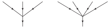
Figure 3: $c_{3}$ and $c_{4}$

Let $C:=\{c_{2}^{(\lambda_{1})}\ ,\ c_{3}^{(\lambda_{2})}\ ,\ ...\ ,\ c_{n}^{(\lambda_{n-1})}\}$ be a set of corollas, where $c_{i+1}^{(\lambda_{i})}$ is the $\lambda_{i}$-copies of $c_{i+1}$ (like $d_{i}^{(\lambda_{i})}$ in Section 2.) Let $TC$ be the set of trees generated by $C$. For example, if $C=\{c_{2},c_{3}\}$,

$$T\{c_{2},c_{3}\}=\{c_{2}\circ_{1}c_{3}\ ,\ c_{2}\circ_{2}c_{3}\ ,\ c_{3}\circ_{1}c_{2}\ ,\ c_{3}\circ_{2}c_{2}\ ,\ c_{3}\circ_{3}c_{2}\}.$$

where $\circ_{i}$ is the grafting product of trees at the $i$th-leaf. Hence the cardinal number of $T\{c_{2},c_{3}\}$ is $5$. The number of leaves of $T\in TC$ is computed as follows.

$$|T|:=\lambda_{1}+2\lambda_{2}+\cdots+(n-1)\lambda_{n-1}+1.$$

Corollary 4.9.

The cardinal number of $TC$ is

$$\mathrm{card}(TC):=\frac{1}{|T|}\binom{|T|+\Lambda-1}{\Lambda}\frac{\Lambda!}{\lambda_{1}!\cdots\lambda_{n-1}!},$$

where $\Lambda=\lambda_{1}+\cdots+\lambda_{n-1}$.

Proof.

$\lambda_{i}$ is equal to the number of $d_{i}$ and $\Lambda=a$. ∎

It is easy to see that $\mathrm{card}(T\{c_{k}^{n}\})$ is the (Fuss-)Catalan number for $k$-ary trees.

– Appendix –

A1 ([3]). Let $X:=S^{c}\sqcup S$ be a wordset decomposed into a subset $S$ and its complement $S^{c}$, and let $\mathcal{F}_{Lie}(X)$ be the free Lie algebra over $X$. Then the following identity holds.

$$\mathcal{F}_{Lie}(X)\cong\mathcal{F}_{Lie}(T)\oplus\mathcal{F}_{Lie}(S),$$

where $T$ is a word set,

$$T:=S^{c}\sqcup(S^{c},S)\sqcup(S^{c},S,S)\sqcup\cdots.$$

And there exists a natural isomorphism,

$$T\cong S^{c}\oplus\{S^{c},S\}\oplus\{\{S^{c},S\},S\}\oplus\cdots.$$

Proof.

$$\mathcal{F}_{Lie}(S^{c}\sqcup S)\cong\frac{\mathcal{F}_{Lie}(T\sqcup S)}{I}\cong\mathcal{F}_{Lie}(T)\oplus\mathcal{F}_{Lie}(S),$$

where $I$ is an ideal generated by the identity, $\{T,S\}-(T,S)=0$. ∎

A2. $\mathcal{L}ie\otimes\mathbf{d}$ is the tree differntial on $\mathbf{s}\mathcal{L}eib_{\infty}$.

Proof.

Recall (1)-(3) the defining equations of the tree differential on $\mathbf{s}\mathcal{L}eib_{\infty}$. It suffices to prove that $\{[d_{i-1},d_{j-1}](1),...,n\}\cong T_{i}T_{j}+T_{j}T_{i}$. The left-hand side expands to

$$\{[d_{i-1},d_{j-1}](1),...,n\}=\{d_{i-1}d_{j-1}(1),...,n\}+\{d_{j-1}d_{i-1}(1),...,n\}$$

and the term is

$$\{d_{i-1}d_{j-1}(1),...,n\}=\{d_{i-1}\{d_{j-1}(1),...,j\},...,n\}+\sum_{k\geq 2}^{j}\{d_{j-1}(1),...,d_{i-1}(k),...,n\},$$ (15)

where the derivation property is used. We denote by $T^{(m)}$ a labeled rooted tree whose most left label is $m$. One can divide $T_{i}T_{j}+T_{j}T_{i}$ into two parts, i.e., the part that $T_{j}$ has the lable $1$ and the other part,

$$T_{i}T_{j}+T_{j}T_{i}=\Big{(}T_{i}T_{j}^{(1)}+T_{j}^{(1)}T_{i}\Big{)}+\Big{(}T_{i}^{(1)}T_{j}+T_{j}T_{i}^{(1)}\Big{)}.$$

The first term has the form of

$$T_{i}T_{j}^{(1)}+T_{j}^{(1)}T_{i}=T_{i}\circ_{1}T_{j}+\sum_{k\geq 2}^{j}T_{i}^{(k)}T_{j}^{(1)}+T_{j}^{(1)}T_{i}^{(k)}.$$ (16)

Obviously $\{d_{i-1}\{d_{j-1}(1),...,j\},...,n\}\cong T_{i}\circ_{1}T_{j}$. It is also easy to see that

$$\{d_{j-1}(1),...,d_{i-1}(k),...,n\}\cong T_{i}^{(k)}T_{j}^{(1)}+T_{j}^{(1)}T_{i}^{(k)},$$

which yields $(\ref{proofa201})\cong(\ref{proofa202})$. ∎

Keywords : derived bracket, Leibniz Loday algebra, operad, homotopy algebra, tree graph, Schröder number.

Kyousuke UCHINO (Freelance)
SAWAYA apartments 103, Yaraicho 9
Shinjyuku Tokyo Japan
email:kuchinon[at]gmail.com

References

- [1] M. Aguiar. Pre-Poisson algebras. Lett. Math. Phys. 54 (2000), no. 4, 263–277.
- [2] M. Ammar and N. Poncin. Coalgebraic approach to the Loday infinity category, stem differential for 2n -ary graded and homotopy algebras. Ann. Inst. Fourier (Grenoble) 60 (2010), no. 1, 355–387.
- [3] N. Bourbaki. Lie Groups and Lie Algebras. (1973) Chapter 2, Section 2, 2, 9, Proposition 10.
- [4] F. Chapoton. Un endofoncteur de la categorie des operades. Lecture Notes in Mathematics 1763. (2001) 105–110.
- [5] V. Ginzburg and M. Kapranov. Koszul duality for operads. Duke Math. J. (1994) 203–272: Erratum to: “Koszul duality for operads”. Duke Math. J. (1995) 293–293.
- [6] Ira M. Gessel. Schröder numbers, large and small. Slide May 2009. http://people.brandeis.edu/~gessel/
- [7] Y. Kosmann-Schwarzbach. From Poisson algebras to Gerstenhaber algebras. Ann. Inst. Fourier (Grenoble). (1996) 1243–1274.
- [8] Y. Kosmann-Schwarzbach. Derived brackets. Lett. Math. Phys. (2004) 61–87.
- [9] J-L. Loday and T. Pirashvili. Universal enveloping algebras of Leibniz algebras and (co)homology. Math. Ann. (1993) 139–158.
- [10] J-L. Loday. La renaissance des operades. Seminaire Bourbaki, Vol. 1994/95. Asterisque No. 237 (1996) Exp. No. 792, 3, 47–74
- [11] J-L. Loday. Dialgebras. Lecture Notes in Mathematics 1763. (2001) 7–66.
- [12] J-L. Loday and B. Vallette. Algebraic Operads. Grundlehren der mathematischen Wissenschaften. 346. Springer-Verlag (2012). 654 pages.
- [13] D. Roytenberg. Quasi-Lie bialgebroids and twisted Poisson manifolds. Lett. Math. Phys. (2002) 123–137.
- [14] D. G. Rogers. A schröder triangle: Three combinatorial problems. Lecture Notes in Mathematics 622. (1977) 175–196.
- [15] B. Vallette. Manin products, Koszul duality, Loday algebras and Deligne conjecture. J. Reine Angew. Math. (2008) 105–164.
- [16] K. Uchino. Derived brackets and Manin products. Lett. Math. Phys. (2010) 37–53.
- [17] K. Uchino. Derived brackets and sh Leibniz algebras. J. Pure Appl. Algebra. (2011) 1102–1111.
- [18] T. Voronov. Higher derived brackets and homotopy algebras. J. Pure Appl. Algebra 202 (2005), no. 1-3, 133–153.
- [19] G. W. Zinbiel. Encyclopedia of types of algebras 2010. arXiv:1101.0267.