FM stars: A Fourier view of pulsating binary stars, a new technique for measuring radial velocities photometrically

Abstract

Some pulsating stars are good clocks. When they are found in binary stars, the frequencies of their luminosity variations are modulated by the Doppler effect caused by orbital motion. For each pulsation frequency this manifests itself as a multiplet separated by the orbital frequency in the Fourier transform of the light curve of the star. We derive the theoretical relations to exploit data from the Fourier transform to derive all the parameters of a binary system traditionally extracted from spectroscopic radial velocities, including the mass function which is easily derived from the amplitude ratio of the first orbital sidelobes to the central frequency for each pulsation frequency. This is a new technique that yields radial velocities from the Doppler shift of a pulsation frequency, thus eliminates the need to obtain spectra. For binary stars with pulsating components, an orbital solution can be obtained from the light curve alone. We give a complete derivation of this and demonstrate it both with artificial data, and with a case of a hierarchical eclipsing binary with Kepler mission data, KIC 4150611 (HD 181469). We show that it is possible to detect Jupiter-mass planets orbiting $\delta$ Sct and other pulsating stars with our technique. We also show how to distinguish orbital frequency multiplets from potentially similar nonradial $m$-mode multiplets and from oblique pulsation multiplets.

1 Introduction

There are many periodic phenomena in astronomy that act as clocks: the Earth’s rotation and orbit, the orbit of the Moon, the orbits of binary stars and exoplanets, the spin of pulsars, stellar rotation and stellar pulsation are examples. All of these astronomical clocks show measurable frequency and/or phase modulation in the modern era of attosecond precision atomic time, and stunning geophysical and astrophysical insight can be gleaned from their frequency variability.

Variations in the Earth’s rotation arise from, for example, changes in seasonal winds, longer-term changes in ocean currents (such as in the El Nino quasi-biennial southern oscillation), monthly changes in the tides, and long-term tidal interaction between the Earth and Moon. Earth rotation even suffers measurable glitches with large earthquakes and internal changes in Earth’s rotational angular momentum. Earth’s rotation and orbit induce frequency variability in all astronomical observations and must be precisely accounted for, usually by transforming times of observations to Barycentric Julian Date (BJD). The astronomical unit is known to an accuracy of less than 5 m, on which scale the Earth’s orbit is not closed and is highly non-Keplerian. Incorrectly transforming to BJD led to the first claim of discovery of an exoplanet (Bailes et al. 1991; it was a rediscovery of Earth), and correct transformation led to the true first exoplanets discovered orbiting the pulsar PSR 1257+12 (Wolszczan & Frail, 1992). Hulse & Taylor (1975) famously discovered the first binary pulsar. Timing variations in its pulses confirmed energy losses caused by gravitational radiation and led to the award of the Nobel prize to them in 1993.

Deviations of astronomical clocks from perfect time keepers have traditionally been studied using ‘Observed minus Corrected’ ($O-C$) diagrams (see, e.g., Sterken 2005 and other papers in those proceedings). Pulsar timings are all studied this way. In an $O-C$ diagram some measure of periodicity (pulse timing in a pulsar, time of periastron passage in a binary star, the phase of one pulsation cycle in a pulsating star) is compared to a hypothetical perfect clock with an assumed period. Deviations from linearity in the $O-C$ diagram can then diagnose evolutionary changes in an orbit or stellar pulsation, apsidal motion in a binary star, stochastic or cyclic variations in stellar pulsation, and, most importantly for our purposes here, periodic Doppler variability in a binary star or exoplanet system.

That some pulsating stars are sufficiently good clocks to detect exoplanets has been demonstrated. In the case of V391 Peg (Silvotti et al., 2007), a 3.2- M${}_{\rm Jupiter}/\sin i$ planet in a 3.2-yr orbit around an Extreme Horizontal Branch star was detected in sinusoidal frequency variations inferred from the $O-C$ diagrams for two independent pulsation modes (where M_Jupiter is the Jovian mass and $i$ denotes the inclination angle of the orbital axis with respect to the line of sight). These frequency variations arise simply as a result of the light time effect.

A barrier to the study of binary star orbits and exoplanet orbits using $O-C$ diagrams has always been the difficulty of precisely phasing cycles across the inevitable gaps in ground-based observations. Great care must be taken not to lose cycle counts across the gaps. The light time effect can also be seen directly in the Fourier transform of a light curve of a pulsating star, where the cycle count ambiguity manifests itself in the aliases in the spectral window pattern. In principle, this method yields all the information in an $O-C$ diagram, but the tradition has been to use $O-C$ diagrams rather than amplitude spectra, probably because of the apparently daunting confusion of multiple spectral window patterns for multiperiodic pulsating stars with large gaps in their light curves.

Now, with spaced-based light curves of stars at $\mu$mag photometric precision and with duty cycles exceeding 90 per cent, e.g., those obtained with the Kepler mission (Koch et al., 2010), not only is there no need to resort to $O-C$ diagrams to study orbital motion from the light curve, it is preferable to do this directly with information about the frequencies derived from the Fourier transform. For pulsating stars that are sufficiently good clocks, it is possible to derive orbital radial velocities in a binary system from the light curve alone – obviating the need for time-consuming spectroscopic observations. The fundamental mass function, $f(m_{1},m_{2},\sin i)={m_{2}^{3}\sin^{3}i}/{(m_{1}+m_{2})^{2}}$, for a binary star can be derived directly from the amplitudes and phases of frequency multiplets found in the amplitude spectrum without need of radial velocities, although those, too, can be determined from the photometric data. Here, $m_{1}$ and $m_{2}$ denote the mass of the pulsating star in the binary system and the mass of the companion, respectively, and $i$ is the inclination angle of the orbital axis with respect to the line of sight.

The Kepler mission is observing about 150 000 stars nearly continuously for spans of months to years. Many of these stars are classical pulsating variables, some of which are in binary or multiple star systems. The study of the pulsations in such stars is traditionally done using Fourier transforms, and it is the patterns in the frequencies that lead to astrophysical inference; see, for example, the fundamental textbooks Unno et al. (1989) and Aerts et al. (2010). One type of pattern that arises is the frequency multiplet. This may be the result of nonradial modes of degree $\ell$ for which all, or some, of the ($2\ell+1$) $m$-mode components (where $-\ell\leq m\leq+\ell$) may be present. The splitting between the frequencies of such multiplets is proportional to stellar angular frequency, hence leads to a direct measure of the rotation velocity of the star averaged over the pulsation cavity (Ledoux, 1951). In the best case of the Sun, this leads to a 2D map (in depth and latitude) of rotation velocity over the outer half of the solar radius. Frequency multiplets also occur for a star that has pulsation modes inclined to the rotation axis, leading to oblique pulsation, as in the roAp stars (e.g., Kurtz 1982; Shibahashi & Takata 1993; Bigot & Kurtz 2011). This, too, leads to a frequency multiplet, in this case split by exactly the rotation frequency of the star.

Other types of frequency modulation may be present in pulsating stars. The Sun is known to show frequency variability correlated with the 11-yr solar cycle. A large fraction of RR Lyr stars exhibit quasi-periodic amplitude and phase modulation known as the Blazhko effect. The physical cause of this remains a mystery after more than a century of study. Benkő et al. (2009) and Benkő et al. (2011) have looked at the formalism of the combination of frequency modulation and amplitude modulation in the context of the Blazhko stars, showing the type of frequency multiplets expected compared to those observed. Their frequency modulation is analogous to that of FM (frequency modulation) radio waves, hence the formalism is well known in the theory of radio engineering, but unfamiliar to most astronomers.

Here we examine FM for pulsating stars in binary star systems. Imagine that one star in a binary system is sinusoidally pulsating with a single frequency. Its luminosity varies with time as a consequence of pulsation. For a single star with no radial velocity with respect to the solar system barycentre, the observed luminosity variation would also be purely sinusoidal and would be expressed in terms of the exact same frequency as the one with which the star is intrinsically pulsating. But, in the case of a binary system, the orbital motion of the star leads a periodic variation in the distance between us and the star; that is, the path length of the light, thus the phase of the observed luminosity variation also varies with the orbital period. This is the light time effect and is equivalent to a periodic Doppler shift of the pulsation frequency. The situation is the same as the case of a binary pulsar. Fig. 1 shows the difference between the light curves in these two cases.

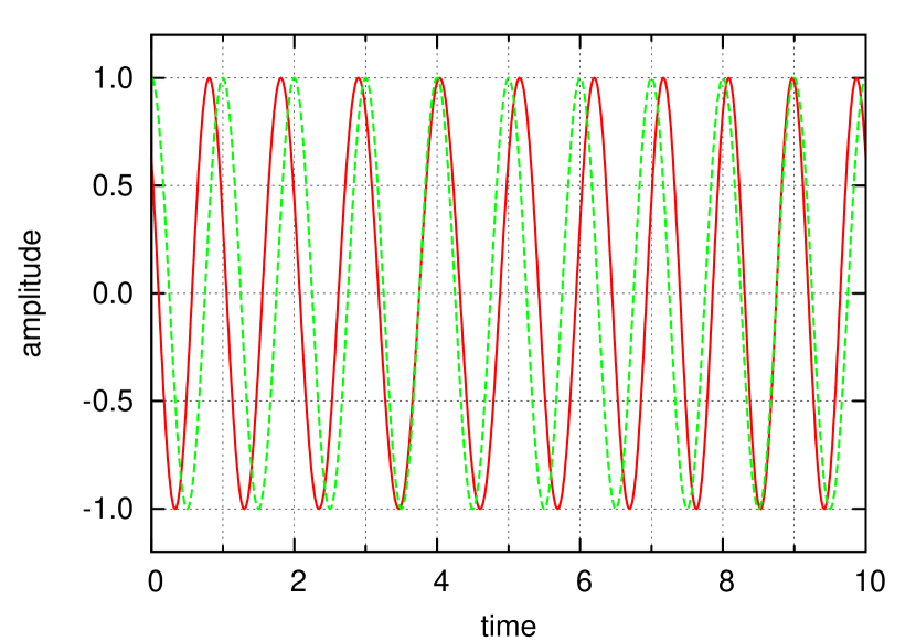
Figure 1: A schematic picture of phase modulation. The green, dashed curve shows a pure sinusoid. The red, solid curve shows the same sinusoid with frequency modulation.

In the following section we show the formal derivations of the light time effect in a binary star on the Fourier transform of the light curve of a pulsating star. This also leads to frequency multiplets in the amplitude spectra of such stars where the frequency splitting is equal to the orbital frequency, and where the amplitudes and phases of the components of the frequency multiplet can be used to derive all of the information traditionally found from radial velocity curves: the time of periastron passage, orbital eccentricity, the mass function, $f(m_{1},m_{2},\sin i)$, and even the radial velocity curve itself. This is a significant advance in the study of binary star orbits; effectively we have photometric radial velocities.

Asteroseismologists must also be aware of the expected frequency patterns for pulsating stars in binary systems. These show a new kind of multiplet in the amplitude spectra that needs to be recognised and exploited. In the common case of binary stars with short orbital periods where rotation is synchronous, the frequency multiplets that we derive here, Ledoux rotational spitting multiplets and oblique pulsation multiplets can potentially be confused, and must be distinguished. We show how this is possible using frequency separation, amplitude ratios and multiplet phase relationships.

2 The simplest case: a binary star with circular orbital motion

2.1 Analytical expression of phase modulation

Let us first consider the simplest case, a pulsating star in a binary with circular orbital motion. We assume that the radial velocity of the centre-of-mass of the binary system with respect to the solar system barycentre – the $\gamma$- velocity – has been subtracted, and we assume that observations are corrected to the solar system barycentre so that there is no component of the Earth’s orbital velocity. We name the stars ‘1’ and ‘2’, and suppose that star 1 is pulsating. In this case, the observed luminosity variation at time $t$ has a form

$$\cos\left\{\omega_{0}\left[t-{{1}\over{c}}\int_{0}^{t}v_{\rm rad,1}(t^{\prime})dt^{\prime}\right]+\phi\right\},$$ (1)

where $\omega_{0}$ is the angular frequency of pulsation, $c$ the speed of light, $v_{\rm rad,1}$ denotes the line of sight velocity of the star 1 due to orbital motion, and $\phi$ is the pulsation phase at $t=0$. The second term in the square bracket measures the arrival time delay of the signal from the star to us. The instantaneously observed frequency is regarded as the time derivative of the phase, which is given by

$$\omega_{\rm obs}=\omega_{0}\left[1-{{v_{\rm rad,1}(t)}\over{c}}\right].$$ (2)

The second term in the right-hand-side of the above equation is the classical Doppler shift of the frequency.

In this section, we adopt the phase at which the radial velocity of star 1 reaches its maximum, i.e. the maximum velocity of recession, as $t=0$. Then, the radial velocity $v_{\rm rad,1}(t)$ is given by

$$v_{\rm rad,1}(t)=a_{1}\Omega\sin i\cos\Omega t,$$ (3)

where $a_{1}$ denotes the orbital radius of star 1, that is, the distance from the star to the centre of gravity of the binary system, $\Omega$ denotes the orbital angular frequency, and $i$ denotes the inclination angle of the orbital axis with respect to the line of sight. Following convention, the sign of $v_{\rm rad,1}$ is defined so that $v_{\rm rad,1}>0$ when the object is receding from us. Hence,

$$\cos\left\{\omega_{0}\left[t-{{1}\over{c}}\int_{0}^{t}v_{\rm rad,1}(t^{\prime})dt^{\prime}\right]+\phi\right\}$$

$$=\cos\left[\left(\omega_{0}t+\phi\right)+{{a_{1}\omega_{0}\sin i}\over{c}}\sin\Omega t\right].$$ (4)

This expression means that the phase is modulated with the orbital angular frequency $\Omega$ and with the amplitude $a_{1}\omega_{0}\sin i/c$. This result is reasonable, since the maximum arrival time delay is $a_{1}\sin i/c$, hence the maximum phase difference is $a_{1}\omega_{0}\sin i/c$.

2.2 An estimate of the amplitude of phase modulation

From Kepler’s 3rd law, the separation between the components 1 and 2 of a binary is

$$a=\left({{G{\rm M}_{\odot}}\over{4\pi^{2}}}\right)^{1/3}\left({{m_{1}}\over{{\rm M}_{\odot}}}\right)^{1/3}(1+q)^{1/3}P_{\rm orb}^{2/3},$$ (5)

where

$$q\equiv{{m_{2}}\over{m_{1}}}$$ (6)

denotes the mass ratio of the stars and

$$P_{\rm orb}\equiv{{2\pi}\over{\Omega}}$$ (7)

denotes the orbital period. Hence, the distance between star 1 and the centre of gravity, $a_{1}$, is

$$a_{1} = q(1+q)^{-1}a$$ (8)

$$= \left({{G{\rm M}_{\odot}}\over{4\pi^{2}}}\right)^{1/3}\left({{m_{1}}\over{{\rm M}_{\odot}}}\right)^{1/3}q(1+q)^{-2/3}P_{\rm orb}^{2/3}.$$

Then, the amplitude of the Doppler frequency shift, $a_{1}\Omega\sin i/c$, is given by

$${{\left(2\pi G{\rm M}_{\odot}\right)^{1/3}}\over{c}}\left({{m_{1}}\over{{\rm M}_{\odot}}}\right)^{1/3}q(1+q)^{-2/3}{P_{\rm orb}}^{-1/3}\sin i$$

$$\simeq 7.1\times 10^{-4}\left({{m_{1}}\over{{\rm M}_{\odot}}}\right)^{1/3}q(1+q)^{-2/3}\left({{P_{\rm orb}}\over{1\,{\rm d}}}\right)^{-1/3}\sin i.$$

This is typically of the order of $10^{-3}$.

The amplitude of phase modulation, $a_{1}\omega_{0}\sin i/c$, is given by

$$\alpha \equiv {{\left(2\pi G{\rm M}_{\odot}\right)^{1/3}}\over{c}}\left({{m_{1}}\over{{\rm M}_{\odot}}}\right)^{1/3}q(1+q)^{-2/3}{{P_{\rm orb}^{2/3}}\over{P_{\rm osc}}}\sin i$$

$$\simeq 1.7\times 10^{-2}\left({{m_{1}}\over{{\rm M}_{\odot}}}\right)^{1/3}q(1+q)^{-2/3}{{(P_{\rm orb}/1\,{\rm d})^{2/3}}\over{(P_{\rm osc}/1\,{\rm h})}}\sin i,$$

where

$$P_{\rm osc}\equiv{{2\pi}\over{\omega_{0}}}$$ (12)

denotes the pulsation period. It should be noted that the amplitude of the phase modulation is not necessarily small; it can be quite large depending on the combination of $P_{\rm orb}$ and $P_{\rm osc}$. In the case of $P_{\rm orb}=1$  d and $P_{\rm osc}=1$ h, the amplitude of phase modulation is of order of $10^{-2}$. Fig. 2 shows the dependence of the phase modulation amplitude, $\alpha$, on $P_{\rm orb}$ and $P_{\rm osc}$ in the case of $m_{1}=1$ M_⊙, $q=1$ and $i=90^{\circ}$.

Larger values of the phase modulation, $\alpha$, are more detectable. It can be seen in Fig. 2 that for a given oscillation period, longer orbital periods are more detectable, and for a given orbital period shorter pulsation periods (higher pulsation frequencies) are more detectable. The combination of the two – high pulsation frequency and long orbital period – gives the most detectable cases. This will be relevant in Section 4 below when we discuss the detectability of exoplanets with our technique.

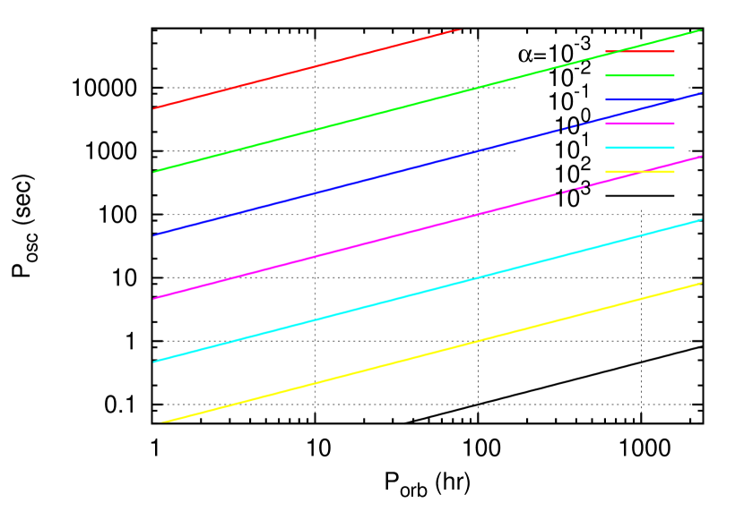
Figure 2: The dependence of the phase modulation amplitude $\alpha$ in the case of $m_{1}=1$ M_⊙, $q=1$, and $i=90^{\circ}$.

2.3 Mathematical formulae

Our aim is to carry out the Fourier analysis of pulsating stars showing phase modulation due to orbital motion in a binary. As deduced from equation (4), the problem is then essentially how to treat the terms $\cos(\alpha\sin\Omega t)$ and $\sin(\alpha\sin\Omega t)$. These terms can be expressed with a series expansion in terms of Bessel functions of the first kind with integer order:

$$\cos(\alpha\sin\Omega t)=J_{0}(\alpha)+2\sum_{n=1}^{\infty}J_{2n}(\alpha)\cos 2n\Omega t$$ (13)

$$\sin(\alpha\sin\Omega t)=2\sum_{n=0}^{\infty}J_{2n+1}(\alpha)\sin(2n+1)\Omega t,$$ (14)

respectively. Here $J_{n}(x)$ denotes the Bessel function of the first kind of integer order $n$:

$$J_{n}(x)=\sum_{k=0}^{\infty}(-1)^{k}{{(x/2)^{n+2k}}\over{(n+k)!\,k!}}.$$ (15)

Fig. 3 illustrates the five lowest-order such functions.

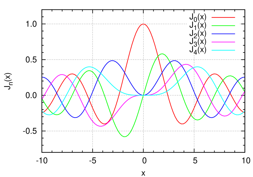
Figure 3: Bessel functions of the first kind with integer order.

Noting that Bessel functions with negative integer orders are defined as

$$J_{-n}(x)=(-1)^{n}J_{n}(x),$$ (16)

we reach an expression of the right-hand side of equation (4) with a series expansion in terms of cosine functions:

$$\cos\left[(\omega_{0}t+\phi)+\alpha\sin\Omega t\right]$$

$$=\sum_{n=-\infty}^{\infty}J_{n}(\alpha)\cos\left[(\omega_{0}+n\Omega)t+\phi\right].$$ (17)

It should be noted that this relation is the mathematical base for the broadcast of FM radio. This relation also has been applied recently to Blazhko RR Lyr stars by Benkő et al. (2009) and Benkő et al. (2011). Vibrato in music is another example that is described by this equation.

It is instructive to write down here, for later use, similar expansions for $\cos(\alpha\cos\Omega t)$ and $\sin(\alpha\cos\Omega t)$ as well:

$$\cos(\alpha\cos\Omega t)=J_{0}(\alpha)+2\sum_{n=1}^{\infty}(-1)^{n}J_{2n}(\alpha)\cos 2n\Omega t$$ (18)

and

$$\sin(\alpha\cos\Omega t)=2\sum_{n=0}^{\infty}(-1)^{n}J_{2n+1}(\alpha)\cos(2n+1)\Omega t.$$ (19)

After the names of two great mathematicians Carl Jacobi and Carl Theodor Anger who derived these series expansions, the expansions (13), (14), (18), and (19) are now called Jacobi-Anger expansions.

2.4 The expected frequency spectrum

2.4.1 General description

Equation (17) means that a frequency multiplet equally split by the orbital frequency $\Omega$ appears in the frequency spectrum of a pulsating star in a binary system with a circular orbit. The orbital period is then determined from the spacing of the multiplet. The amplitude ratio of the $n$-th side peak to the central peak is given by

$${{A_{+n}+A_{-n}}\over{A_{0}}}={{2|J_{n}(\alpha)|}\over{|J_{0}(\alpha)|}},$$ (20)

where $A_{+n}$, $A_{-n}$ and $A_{0}$ represent the amplitudes of the peaks at $\omega_{0}+n\Omega$, $\omega_{0}-n\Omega$, and $\omega_{0}$, respectively. Fig. 4 shows the amplitude ratio of the $n$-th peak to the central peak as a function of the phase modulation amplitude $\alpha$.

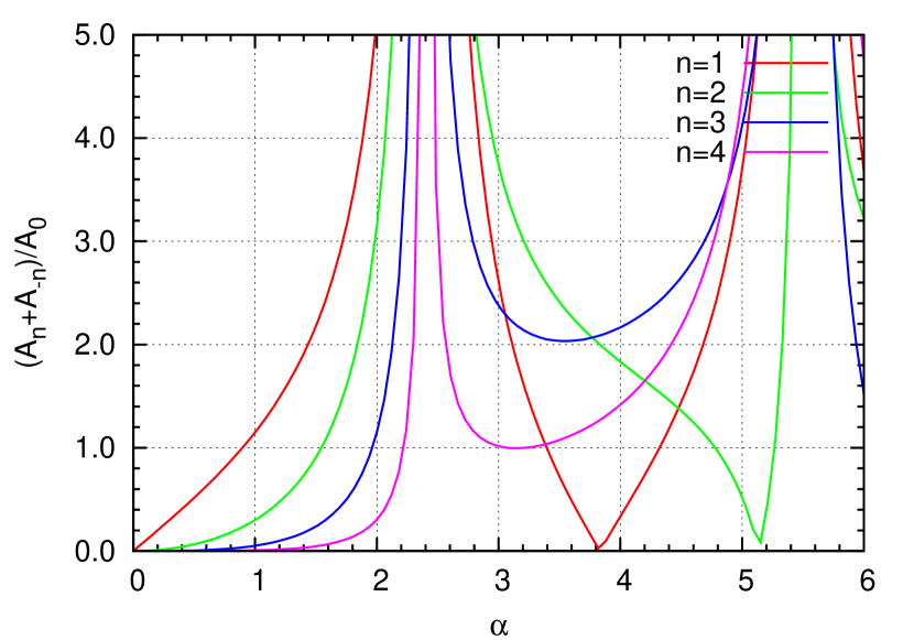
Figure 4: The amplitude ratio of the $n$-th side peaks to the central peak of the multiplet frequency spectrum, as a function of the phase modulation amplitude $\alpha$. $A_{\pm n}$ and $A_{0}$ denote the amplitude of the frequencies at $\omega_{0}\pm n\Omega$ and $\omega_{0}$, respectively.

The multiplet is an infinite fold, but the dominant peaks are highly dependent on the value of $\alpha$. For example, in the case of an 0.5-M_⊙ sdB star pulsating with $P_{\rm osc}=150\,{\rm s}$ and orbiting with $P_{\rm orb}=0.1\,{\rm d}$ with the same mass companion, $\alpha\sim 0.04$ and we expect $J_{0}({\alpha})\simeq 1$, $J_{1}({\alpha})\sim\alpha/2\sim 2\times 10^{-2}$, and $J_{n}(\alpha)\sim 0$ for $n\geq 2$. In this case we expect a triplet structure, for which the central component, corresponding to $n=0$ with a frequency $\omega_{0}$, is the highest, and the side peaks, separated from the central peak by $\Omega$, are of the order of $2\times 10^{-2}$ the amplitude of the central peak. However, if the same star is orbiting with $P_{\rm orb}=12.5\,{\rm d}$, then $\alpha\simeq 1$. In this case, $J_{1}({\alpha})/J_{0}({\alpha})\sim 1$ and $J_{2}({\alpha})/J_{0}({\alpha})\sim 0.3$ so that $(A_{+1}+A_{-1})/{A_{0}}\sim 2$ and $(A_{+2}+A_{-2})/{A_{0}}\sim 0.6$; the contribution of $J_{2}(\alpha)$ is not negligible, and a quintuplet structure with an equal spacing of $\Omega$ is expected. As seen in Fig. 4, for $\alpha\gtrsim 0.9$ the side peaks could have higher amplitude than the central component.

Importantly, the phases of the components of the multiplet are such that the sidelobes never modify the total amplitude. At orbital phases $\pi/2$ and $3\pi/2$, when the stars have zero radial velocity, the sidelobes are in phase with each other, but in quadrature, $\pm\pi/2$ radians out of phase with the central peak; at orbital phases 0 and $\pi$, when the star reaches maximum or minimum radial velocity, the sidelobes are $\pi$ radians out of phase with each other and cancel. Thus only frequency modulation occurs with no amplitude modulation, as we expect from our initial conditions. It is these phase relationships that distinguish frequency modulation multiplets from amplitude modulation multiplets, where all members of the multiplet are in phase at the time of amplitude maximum.

2.4.2 Derivation of the binary parameters

From the frequency spectrum we can derive the value of $\alpha$, which is, as seen in equation (LABEL:eq:10),

$$\alpha=\left({{2\pi G}\over{c}}\right)^{1/3}{{P_{\rm orb}^{2/3}}\over{P_{\rm osc}}}{{m_{2}\sin i}\over{(m_{1}+m_{2})^{2/3}}}.$$ (21)

Since $P_{\rm osc}$ is observationally known and $P_{\rm orb}$ is also determined from the spacing of the multiplet, the mass function, which is usually derived from spectroscopic measurements of radial velocity in a binary system, is eventually derived from photometric observations through $\alpha$:

$$f(m_{1},m_{2},\sin i) \equiv {{m_{2}^{3}\sin^{3}i}\over{(m_{1}+m_{2})^{2}}}$$ (22)

$$= \alpha^{3}\frac{P_{\rm osc}^{3}}{P_{\rm orb}^{2}}\frac{c^{3}}{2\pi G}.$$

The distance between the star 1 and the centre of gravity is also deduced from $\alpha$:

$$a_{1}\sin i={{P_{\rm osc}}\over{2\pi}}\alpha c,$$ (23)

as is the radial velocity:

$$v_{\rm rad,1}(t)={{P_{\rm osc}}\over{P_{\rm orb}}}\alpha c\cos\Omega t.$$ (24)

2.4.3 The case of $\alpha\ll 1$

Most binary stars have $\alpha\ll 1$. In this case, $J_{1}(\alpha)\simeq\alpha/2$, and the value of $\alpha$ is derived to be

$$\alpha={{A_{+1}+A_{-1}}\over{A_{0}}}.$$ (25)

Then, the mass function, the distance between the star and the centre of gravity, and the radial velocity are derived to be

$$f(m_{1},m_{2},\sin i)=\left(\frac{A_{+1}+A_{-1}}{A_{0}}\right)^{3}\frac{P_{\rm osc}^{3}}{P_{\rm orb}^{2}}\frac{c^{3}}{2\pi G},$$ (26)

$$a_{1}\sin i={{P_{\rm osc}}\over{2\pi}}{{A_{+1}+A_{-1}}\over{A_{0}}}c,$$ (27)

and

$$v_{\rm rad,1}(t)={{P_{\rm osc}}\over{P_{\rm orb}}}{{A_{+1}+A_{-1}}\over{A_{0}}}c\cos\Omega t.$$ (28)

2.5 An example with artificial data for the case of a circular orbit

We illustrate the results derived in the previous subsection with artificial data generated for the following parameters: $m_{1}=1.7$ M_⊙ and $\nu_{\rm osc}\equiv 1/P_{\rm osc}=20$ d^-1 – typical of a late-A $\delta$ Sct star; $e=0$, of course; $m_{2}=1$ M_⊙; $P_{\rm orb}=10$ d; and $i=90^{\circ}$. In this case our parameter $\alpha=3.39\times 10^{-2}$ (see equation (LABEL:eq:10) and Fig. 2). Fig. 5 shows the radial velocity curve for this system where our convention is the star 1 – the pulsating A star – is at maximum velocity of recession at phase zero. These represent a typical eclipsing binary $\delta$ Sct Am star. (The reason we say Am star in this case is that most A star binary systems with $P_{\rm orb}=10$ d have synchronous rotation, leading to the slow rotation that is a prerequisite for atomic diffusion in metallic-lined A stars.)

We have generated an artificial light curve with no noise using 10 points per pulsation cycle and a time span of 10 orbital periods (100 d) in a hare-and-hound test to see how well the input binary parameters are reproduced from the light curve. The top panel of Fig. 6 shows an amplitude spectrum of the generated light curve around the chosen pulsation frequency, 20 d^-1. The first sidelobes at 19.9 d^-1 and 20.1 d^-1 are barely visible in this panel, but are clearly seen after prewhitening the central peak as shown in the bottom panel of Fig. 6. They are separated from that central peak by 0.1 d^-1 and to have relative amplitudes of 0.017. The orbital period, 10 d, is well determined from the spacing. From the amplitude ratio, the value of $\alpha$ is also reasonably well reproduced.

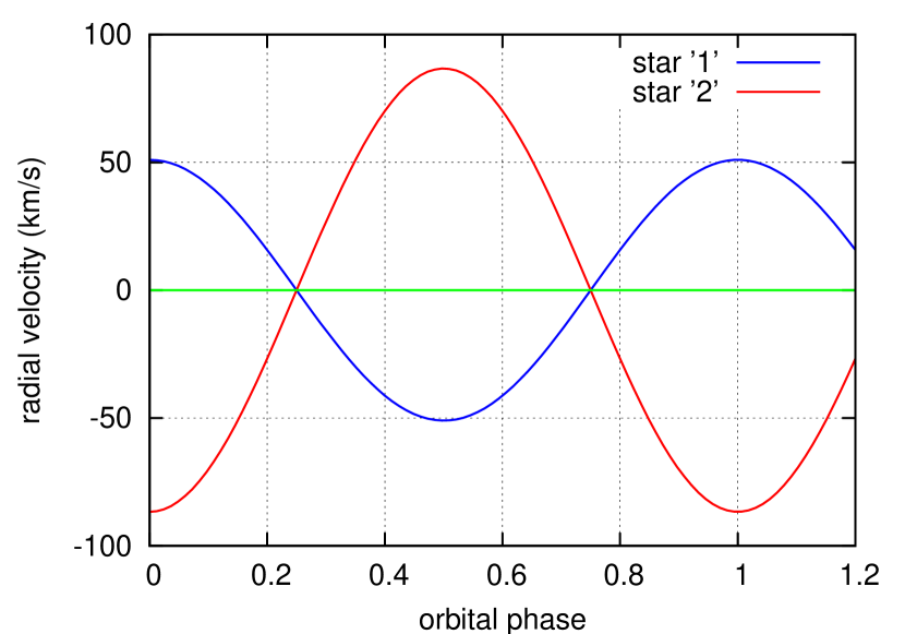
Figure 5: An artificial radial velocity curve for a binary system with a 1.7-M_⊙ $\delta$ Sct star in a 10-d circular orbit with a 1-M_⊙ companion; $i=90^{\circ}$. The blue curve is for the primary component and the red curve the secondary.

Figure 6: Top panel: An amplitude spectrum of the artificial data around the chosen pulsation frequency of 20 d^-1. The amplitude has been chosen to be in intensity units. The first sidelobes at $\pm\nu_{\rm orb}\,(\equiv\pm 1/P_{\rm orb})$ are barely visible. Bottom panel: The amplitude spectrum after prewhitening by the central peak of the multiplet. The two first sidelobes are evident with amplitudes of 0.017 of the amplitude of the central peak. The second sidelobes are insignificant.

Table 1: Least squares fit of the frequency triplet to the artificial data at the orbital phase of eclipse for the orbital parameters given in Section 2.5. The two sidelobes are in phase with each other, but $90^{\circ}$ out of phase with the central peak, as expected. The frequencies are split by the orbital frequency, given $P_{\rm orb}=10$ d. These are artificial data with no noise added, hence there are no errors.

frequency	amplitude	phase
d-1		radians
19.9	0.017	1.57
20.0	1.000	0.00
20.1	0.017	1.57

From the amplitude ratio in Table 1 and equation (22) we derive $f(m_{1},m_{2},\sin i)=0.137\,{\rm M}_{\odot}$, as expected for the input parameters of $i=90^{\circ}$, $m_{1}=1.7\,{\rm M}_{\odot}$ and $m_{2}=1.0\,{\rm M}_{\odot}$. Hence we have shown that the mass function can be derived entirely from the photometric light curve. The expected radial velocity of star 1 is derived from equation (24), from which its amplitude is determined to be 51 km s^-1. Hence the radial velocity curve, shown with the blue curve in Fig. 5, has also been well reproduced only from the photometric light curve.

2.6 An actual example for the case of a circular orbit: the hierarchical multiple system KIC 4150611 = HD 181469

Let us now look at an actual example. The Kepler mission is observing about 150 000 stars over its 115 square degree field-of-view for time spans of one month to years. In the data for Kepler ‘quarters’ (1/4 of its 372-d heliocentric orbit) Q1 to Q9 we can see a hierarchical multiple star system of complexity and interest, KIC 4150611. This system is composed of an eccentric eclipsing binary pair of G stars in an 8.6-d orbit that are a common proper motion pair with a $\delta$ Sct A star in a circular orbit about a pair of K stars with an orbital period of $94.1\pm 0.1$ d; the K star binary itself has an orbital period of about 1.5 d. These five stars show a remarkable set of eclipses, successfully modelled by the Kepler eclipsing binary star working group (Prša et al., in preparation). Here we show that we can derive the mass function for the A star – K-binary system from the light curve alone by using the $\delta$ Sct pulsations as a clock. This is an important advance for a system such as this. Measuring radial velocities from spectra requires a great effort at the telescope to obtain the spectra. Relatively low accuracy then results from spectral disentangling of the A star from the other components of the system, and as a consequence of the rotational velocity of the A star of $v\sin i\sim 100$ km s^-1. Using our technique the A star is the only pulsating star in the system, hence the photometric radial velocities come naturally from just the A star primary and we are unaffected by rotational broadening or spectral disentangling.

Figure 7: An amplitude spectrum for the Q1 to Q9 Kepler long cadence data in the $\delta$ Sct frequency range of the A-star component of the multiple system KIC 4150611. The four peaks are from independent, low overtone modes.

The data we use are Q1 to Q9 long cadence Kepler data with integration times of 29.4 min covering a time span of 774 d. The Nyquist frequency for these data is about 24.5 d^-1. We also have short cadence Kepler data for this star (integration times of 58.9 s) that show the $\delta$ Sct pulsations have frequencies less than the long cadence Nyquist frequency. We have masked the eclipses in the light curve and run a high-pass filter, leaving only the $\delta$ Sct pulsation frequencies. Fig. 7 shows an amplitude spectrum for these data where four peaks stand out. Broad-band photometric data from the Kepler Input Catalogue photometry suggests $T_{\rm eff}\approx 6600$ K and $\log g=4$ (in cgs units) for this star, but this temperature is likely to be underestimated because of the light of the cooler companion stars. We therefore estimate that the A star has a spectral type around the cool border of the $\delta$ Sct instability strip, $T_{\rm eff}\sim 7400$ K.

Table 2: A non-linear least-squares fit of the four highest amplitude frequencies seen in Fig. 7 to the Q1 to Q9 Kepler data for KIC 4150611. The range of frequencies suggests low overtone modes. The zero point in time for the phase is BJD 2455311.758.

frequency	amplitude	phase
d-1	mmag	radians
$17.746558\pm 0.000008$	$0.640\pm 0.007$	$\phantom{-}1.894\pm 0.011$
$18.480519\pm 0.000007$	$0.699\pm 0.007$	$-0.029\pm 0.010$
$20.243260\pm 0.000003$	$1.610\pm 0.007$	$\phantom{-}2.360\pm 0.004$
$22.619577\pm 0.000004$	$1.294\pm 0.007$	$\phantom{-}0.150\pm 0.005$

Table 3: A least squares fit of the frequency triplets for the four high amplitude modes to the Q1 to Q9 Kepler data for KIC 4150611. The frequencies of the multiplets are separated by the orbital frequency. The zero point for the phases has been chosen to be a time of transit of the A star by its companions, $t_{0}={\rm BJD}\,2455311.758$. Column 4 shows that the phases of the sidelobes are equal within the errors at this time and column 5 shows that they are $\pi/2=1.57$ radians out of phase with the central peak. Column 6 shows the amplitude ratios of the sidelobes to the central peaks. Since they are small compared to unity, they are equal to $\alpha$ to great accuracy. The ratios of $\alpha$ to the frequency are the same for all modes, as shown in column 7. The phase relations and amplitude ratios are as expected from our theory.

frequency	amplitude	phase	$\phi_{+1}-\phi_{-1}$	${\langle\phi_{+1}-\phi_{-1}\rangle}-{\phi_{0}}$	$\frac{A_{+1}+A_{-1}}{A_{0}}$	$\alpha/\nu_{\rm osc}$
d-1	mmag	radians	radians	radians		$\times 10^{-3}$ d
17.735937	$0.049\pm 0.007$	$\phantom{-}0.299\pm 0.139$
17.746558	$0.640\pm 0.007$	$\phantom{-}1.892\pm 0.011$	$-0.04\pm 0.24$	$-1.61\pm 0.12$	$0.133\pm 0.016$	$7.49\pm 0.90$
17.757179	$0.036\pm 0.007$	$\phantom{-}0.258\pm 0.191$
18.469898	$0.050\pm 0.007$	$-1.654\pm 0.136$
18.480519	$0.699\pm 0.007$	$-0.031\pm 0.010$	$\phantom{-}0.04\pm 0.20$	$-1.60\pm 0.10$	$0.139\pm 0.014$	$7.52\pm 0.75$
18.491140	$0.047\pm 0.007$	$-1.617\pm 0.147$
20.232639	$0.117\pm 0.007$	$\phantom{-}0.812\pm 0.058$
20.243260	$1.610\pm 0.007$	$\phantom{-}2.358\pm 0.004$	$-0.11\pm 0.08$	$-1.60\pm 0.40$	$0.148\pm 0.006$	$7.31\pm 0.30$
20.253881	$0.122\pm 0.007$	$\phantom{-}0.699\pm 0.056$
22.608956	$0.106\pm 0.007$	$-1.441\pm 0.065$
22.619577	$1.294\pm 0.007$	$\phantom{-}0.147\pm 0.005$	$-0.04\pm 0.09$	$-1.61\pm 0.47$	$0.162\pm 0.008$	$7.16\pm 0.35$
22.630198	$0.104\pm 0.007$	$-1.485\pm 0.066$

Table 2 shows the frequencies, amplitudes and phases for the four peaks seen in Fig. 7. For a first estimate of mode identification, it is useful to look at the $Q$ value for each of the four frequencies. This is defined to be

$$Q={P_{\rm osc}}\sqrt{\frac{\overline{\rho}}{\overline{\rho_{\odot}}}}$$ (29)

where $P_{\rm osc}$ is the pulsation period and $\overline{\rho}$ is the mean density; $Q$ is known as the ‘pulsation constant’. Equation (29) can be rewritten as

$$\log Q=-6.454+\log P_{\rm osc}+\frac{1}{2}\log g+\frac{1}{10}M_{\rm bol}+\log T_{\rm eff},$$ (30)

where $P_{\rm osc}$ is given in d, $\log g$ uses cgs units and $T_{\rm eff}$ is in Kelvin. Using $T_{\rm eff}=7400$ K and $\log g=4.0$, and estimating the bolometric magnitude to be about 2 gives $Q$ values in the range 0.019 to 0.023. Standard values for $\delta$ Sct models are $Q=0.033$ for the fundamental mode and $Q=0.025$ for the first overtone, thus suggesting that the four modes so far examined have radial overtones higher than that. There are additional pulsation mode frequencies of low amplitude that are not seen at the scale of this figure. Those will be examined in detail in a future study.

What we wish to examine here are the sidelobes to these four highest amplitude peaks. Each of these shows a frequency triplet split by the orbital frequency. The highest amplitude peak at 20.243260 d^-1 also has another pulsation mode frequency nearby, so we illustrate the triplets with the simpler example of the second-highest peak at 22.619577 d^-1 as shown in Fig. 8.

There is clearly an equally spaced triplet for this frequency, and this is the case for all four mode frequencies. Table 3 shows a least-squares fit of the frequency triplets for the four modes. After fitting the data by nonlinear least-squares with the four triplets and showing that the frequency spacing is the same within the errors in all cases, we forced each triplet to have exactly equal spacing with a separation of the average orbital frequency determined from all four triplets. To examine the phase relationship of the triplet components, it is important to have exactly equal splitting because of the many cycles back to the time zero point. From the separation of the triplet components, we derive the orbital period of the star is $94.09\pm 0.11$ d.

Figure 8: Top panel: An amplitude spectrum for the Q1 to Q9 KIC 4150611 data centred on the peak at 22.619577 d^-1. Bottom panel: An amplitude spectrum after the central peak has been prewhitened, showing the two sidelobes split from the central peak by exactly the orbital frequency.

It can be seen in Table 3 that the data are an excellent fit to our theory. The zero point in time has been selected to be a time of transit in this eclipsing system as seen in the light curve. The expectation is that the sidelobes should be in phase at this time and exactly $\pi/2$ radians out of phase with the central peak. That is the case for all four triplets. Since the amplitude ratios of the sidelobes to the central peaks of each triplet are small compared to unity, they are regarded as $\alpha$ with great accuracy. It is expected that the ratio of $\alpha$ to the frequency is the same for all triplets, since this is directly proportional to the mass function, as in equation (22). Table 3 shows that this is the case. By using the values obtained for $\alpha$, $P_{\rm orb}$ and $P_{\rm osc}$, we deduce the projected radius of the orbit, $a_{1}\sin i$, the radial velocity, $v_{\rm rad,1}$ and the mass function. Table 4 gives these values derived from each triplet. The consistency of the values for the four independent pulsation frequencies is excellent.

Table 4: The values of $a_{1}\sin i$, the amplitude of the radial velocity and the mass function derived from each triplet. The consistency of the values derived for the four triplets is substantially better than the formal errors might lead us to expect, suggesting that those formal errors may be overestimated.

frequency	$a_{1}\sin i$	RV amplitude	$f(m_{1},m_{2},\sin i)$
d-1	au	km s-1	M⊙
17.746558	$1.30\pm 0.16$	$23.9\pm 2.9$	$0.132\pm 0.116$
18.480519	$1.30\pm 0.13$	$23.9\pm 2.4$	$0.133\pm 0.098$
20.243260	$1.27\pm 0.05$	$23.3\pm 1.0$	$0.124\pm 0.035$
22.619577	$1.24\pm 0.06$	$22.8\pm 1.1$	$0.116\pm 0.034$

Because of the better signal-to-noise ratio for the two highest amplitude frequencies, we derive from them a best estimate of the mass function of $f(m_{1},m_{2},\sin i)=0.120\pm 0.024$ M_⊙. If instead of propagating errors we take the average and standard deviation of the four values of the mass function from Table 4, this gives a value of $f(m_{1},m_{2},\sin i)=0.126\pm 0.008$ M_⊙. Assuming a mass of $M\sim 1.7$ M_⊙ for the A star then gives a total mass for the two K stars of the 1.5-d binary companion (see Prša et al., in preparation) less than 1 M_⊙. We have determined the mass function in KIC 4150611 entirely from the photometric light curve by using the $\delta$ Sct pulsations as clocks and extracting the information from the light time effect by means of the Fourier transform. This is a significant improvement to what can be done for this star with spectroscopic radial velocities.

Fig. 9 shows the radial velocity curves of KIC 4150611 derived from the four sets of multiplets. Note that the differences are small. This result will be tested by comparison with the radial velocities obtained with spectroscopic observations by Prša et al. (in preparation). An advantage of the present analysis is that photometric observations by Kepler have covered a long time span with few interruptions. The duty cycle is far superior to what is currently possible with spectroscopic observations.

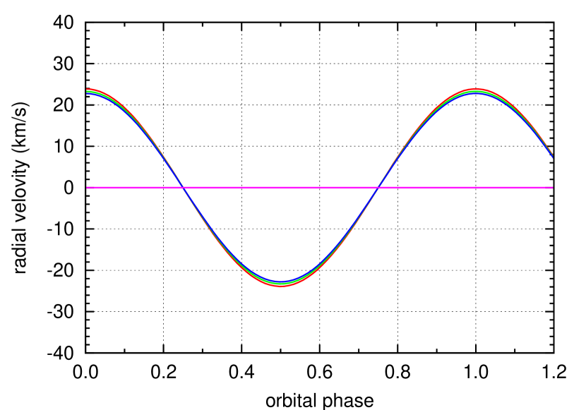
Figure 9: The radial velocity curves of KIC 4150611 derived entirely from the photometric light curve by using the $\delta$ Sct pulsations as clocks and extracting the information from the light time effect by means of the Fourier transform. Note that different curves correspond to different multiplets, but the differences are small.

So far we have assumed that the A-star-K-binary system of KIC 4150611 has a circular orbit. How do we justify this assumption? To find out, we now return to the theory for cases more complex than a circular orbit.

3 The theory for the general case of eccentric orbits

Now let us consider a more realistic case: elliptical orbital motion. The radial velocity curve deviates from a pure sinusoidal curve with a single period. Instead of a simple sinusoid, it is expressed with a Fourier series of the harmonics of the orbital period.

3.1 Radial velocity along the line of sight

Let the $xy$-plane be tangent to the celestial sphere, and let the $z$-axis, being perpendicular to the $xy$-plane and passing through the centre of gravity of the binary, be along the line of sight toward us. The orbital plane of the binary motion is assumed to be inclined to the $xy$-plane by the angle $i$. The orbit is an ellipse. We write the semi-major axis and the eccentricity of the orbit as $a_{1}$ and $e$, respectively. Let $\varpi$ be the angle between the ascending node, which is an intersection of the orbit and the $xy$-plane, and the periapsis. Also let $f$ be the angle between the periapsis and the star at the moment, that is the ‘true anomaly’, and let $r$ be the distance between the centre of gravity and the star (see Fig. 10).

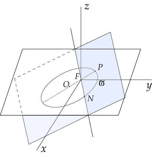
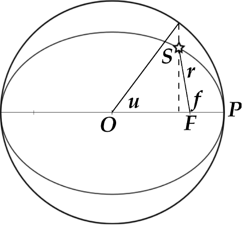
Figure 10: Geometrical configuration. Top: The $xy$-plane is tangent to the celestial sphere, and the $z$-axis is the line of sight toward us. The origin ‘F’ is the focus of the orbital ellipse; that is, the centre of gravity of the binary system. The orbital plane is inclined to the $xy$-plane by the angle $i$. The periapsis of the ellipsoidal orbit is ‘P’, and the ascending node is ‘N’. The angle NFP is $\varpi$. Bottom: Schematic top view (i.e., along the normal to the orbital plane) of the orbital plane. The star is located, at this moment, at ‘S’ on the orbital ellipse, for which the focus is ‘F’. The semi-major axis is $a_{1}$ and the eccentricity is $e$. Then $\overline{{\rm OF}}$ is $a_{1}e$. The distance between the focus, F, and the star, S, is $r$. The angle PFS is ‘the true anomaly’, $f$. ‘The eccentric anomaly’, $u$, is defined through the circumscribed circle that is concentric with the orbital ellipse.

Then, the $z$-coordinate of the position of the star is written as

$$z=r\sin(f+\varpi)\sin i.$$ (31)

The radial velocity along the line of sight, $v_{\rm rad,1}=-{\rm d}z/{\rm d}t$, is then

$$v_{\rm rad,1}=-\left[{{{\rm d}r}\over{{\rm d}t}}\sin(f+\varpi)+r{{{\rm d}f}\over{{\rm d}t}}\cos(f+\varpi)\right]\sin i.$$ (32)

It should be noted here again that the sign of $v_{\rm rad,1}$ is defined so that $v_{\rm rad,1}>0$ when the star is receding from us. The distance $r$ between the focus ‘F’ and the star ‘S’ is expressed with help of a combination of the semi-major axis $a_{1}$, the eccentricity $e$ and the true anomaly $f$:

$$r={{a_{1}(1-e^{2})}\over{1+e\cos f}}.$$ (33)

From the known laws of motion in an ellipse (see text books; e.g., Brouwer & Clemence 1961), we have

$$r{{{\rm d}f}\over{{\rm d}t}}={{a_{1}\Omega(1+e\cos f)}\over{\sqrt{1-e^{2}}}}$$ (34)

and

$${{{\rm d}r}\over{{\rm d}t}}={{a_{1}\Omega e\sin f}\over{\sqrt{1-e^{2}}}}.$$ (35)

Therefore, the radial velocity of the star 1 along the line of sight is expressed as

$$v_{\rm rad,1} = -{{\Omega a_{1}\sin i}\over{\sqrt{1-e^{2}}}}\,\left[\cos(f+\varpi)+e\cos\varpi\right]$$ (37)

$$= -(2\pi G{\rm M}_{\odot})^{1/3}\left({{m_{1}}\over{{\rm M}_{\odot}}}\right)^{1/3}q(1+q)^{-2/3}P_{\rm orb}^{-1/3}\sin i$$

$$\times{{1}\over{\sqrt{1-e^{2}}}}\,\left(\cos f\cos\varpi-\sin f\sin\varpi\right.$$

$$\left.+e\cos\varpi\right).$$

In the case of $e=0$, the periapsis is not uniquely defined, nor are the angles $\varpi$ and $f$. Instead, the angle between the ascending node and the star at the moment, $(f+\varpi)$, is well defined. If we choose $\varpi=\pi$, $f$ means the angle between the descending node and the star at the moment.

3.2 Phase modulation

3.2.1 General formulae

To evaluate phase modulation, we have to integrate the radial velocity with respect to time. The time dependence of radial velocity is implicitly expressed by the true anomaly $f$, which can be written in terms of ‘the eccentric anomaly’, $u$ (see Fig. 10), defined through the circumscribed circle that is concentric with the orbital ellipse, as

$$\cos f={{\cos u-e}\over{1-e\cos u}}.$$ (38)

Kepler’s equation links the eccentric anomaly $u$ with ‘the mean anomaly’ $l$:

$$l \equiv \Omega(t-t_{0})$$ (39)

$$= u-e\sin u,$$

where $t_{0}$ denotes the time of periapsis passage. Various methods of solving Kepler’s equation to obtain $u$ for a given $l$ have been developed. One of them is Fourier expansion. In this method, for a given $l$, $u$ is written as

$$u=l+2\sum_{n=1}^{\infty}{{1}\over{n}}J_{n}(ne)\sin nl.$$ (40)

This expansion converges for any value of $e<1$. With the help of this expansion, the trigonometric functions of the true anomaly $f$ are expressed in terms of the mean anomaly $l$:

$$\cos f=-e+{{2(1-e^{2})}\over{e}}\sum_{n=1}^{\infty}J_{n}(ne)\cos nl$$ (41)

$$\sin f=2\sqrt{1-e^{2}}\sum_{n=1}^{\infty}J_{n}^{\prime}(ne)\sin nl,$$ (42)

where $J_{n}^{\prime}(x)$ denotes ${\rm d}J_{n}(x)/{\rm d}x$. Hence,

$$v_{\rm rad,1} = -(2\pi G{\rm M}_{\odot})^{1/3}\left({{m_{1}}\over{{\rm M}_{\odot}}}\right)^{1/3}q(1+q)^{-2/3}P_{\rm orb}^{-1/3}\sin i$$ (43)

$$\times\,\left[{{2\sqrt{1-e^{2}}}\over{e}}\sum_{n=1}^{\infty}J_{n}(ne)\cos nl\cos\varpi\right.$$

$$\left.-\sum_{n=1}^{\infty}2J_{n}^{\prime}(ne)\sin nl\sin\varpi\right].$$

Note that, although $e$ appears in the denominator, $e=0$ is not singular because $J_{n}(ne)$ reaches zero faster than $e$ itself as $e\rightarrow 0$.

Introducing

$$a_{n}(e)\equiv{{2\sqrt{1-e^{2}}}\over{e}}{{1}\over{n}}J_{n}(ne)$$ (44)

and

$$b_{n}(e)\equiv{{2}\over{n}}J_{n}^{\prime}(ne),$$ (45)

and with the help of equation (39), we eventually obtain

$${{\omega_{0}}\over{c}}\int_{t_{0}}^{t}v_{\rm rad,1}\,{\rm d}t^{\prime}$$

$$=\alpha\left\{\sum_{n=1}^{\infty}\xi_{n}(e,\varpi)\sin\left[n\Omega(t-t_{0})+\vartheta_{n}(e,\varpi)\right]\right.$$

$$+\tau(e,\varpi)\bigg{\}},$$ (46)

where

$$\xi_{n}(e,\varpi)=\sqrt{a_{n}^{2}\cos^{2}\varpi+b_{n}^{2}\sin^{2}\varpi},$$ (47)

$$\vartheta_{n}(e,\varpi)=\tan^{-1}\left({{b_{n}}\over{a_{n}}}\tan\varpi\right)$$ (48)

and

$$\tau(e,\varpi)=-\sum_{n=1}^{\infty}b_{n}\sin\varpi,$$ (49)

and $\alpha$ is defined by equation (LABEL:eq:10). Fig. 11 shows $a_{n}(e)$ and $b_{n}(e)$ as functions of $e$.

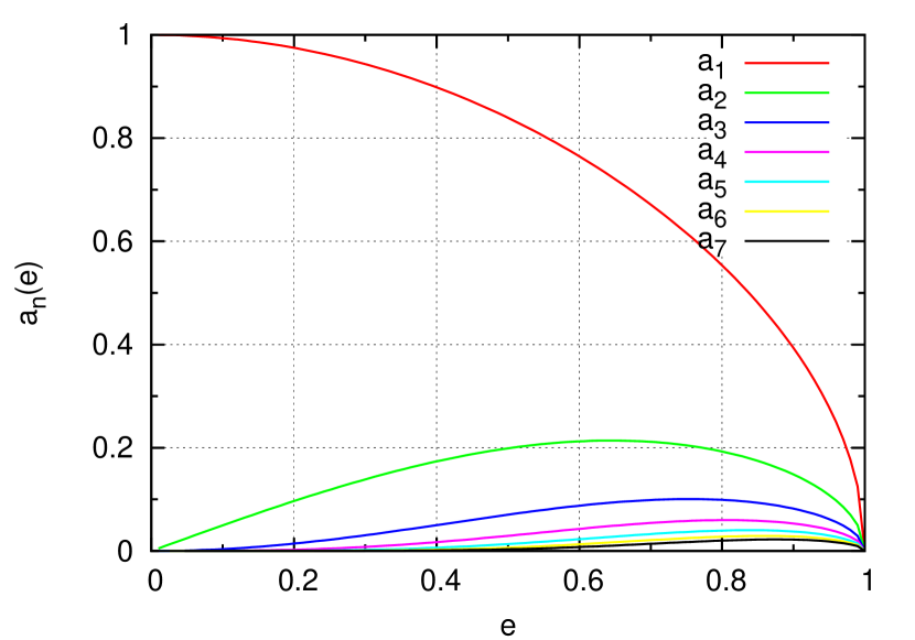
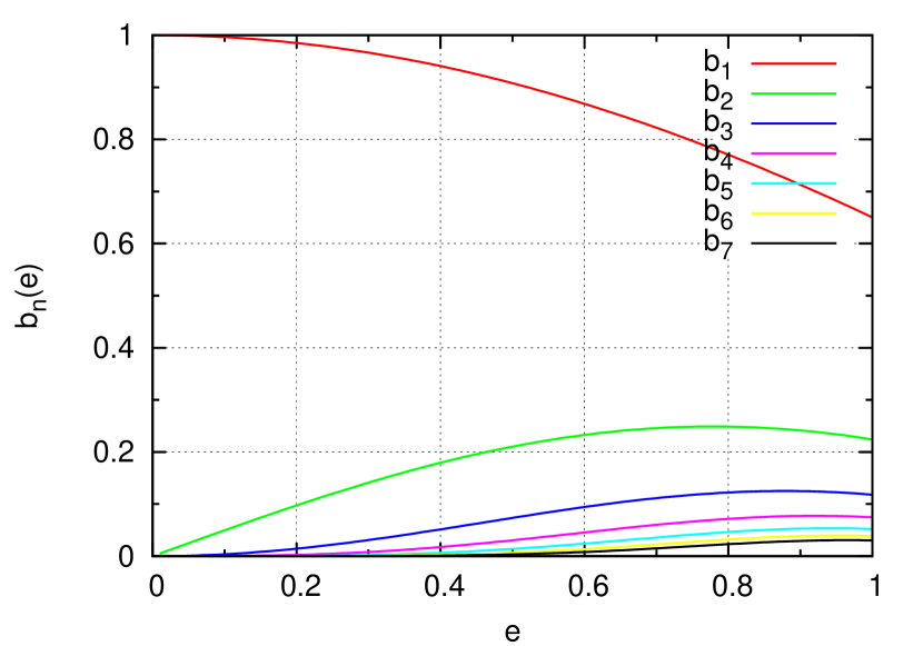
Figure 11: Top panel: $a_{n}=2e^{-1}(1-e^{2})^{1/2}n^{-1}J_{n}(ne)$ as a function of $e$. Bottom panel: $b_{n}=2n^{-1}J_{n}^{\prime}(ne)$ as a function of $e$.

The difference in phase modulation between the circular orbit and ellipsoidal ones is that the former is expressed by a single angular frequency $\Omega$ while the latter is composed of harmonics of $\Omega$. This is of course naturally expected. In the series expansion in equation (46), the terms of $n=1$ dominate over the higher-order terms, but, in the case of $e\gtrsim 0.5$ and $\varpi\sim\pi/2$, the contribution of the higher-order terms becomes non-negligible.

3.2.2 In the limiting cases of $e=0$

One might worry whether the series-expansion form given in the above formally tends to the results obtained in the circular orbital case in the limit of $e\rightarrow 0$. In this section, we prove that it does. As $e\rightarrow 0$, equation (37) is reduced to

$$v_{\rm rad,1}=-\Omega a_{1}\cos(f+\varpi)\sin i.$$ (50)

It should be remembered that in the case of $e=0$, the angle $\varpi$ can be arbitrarily chosen, while $(f+\varpi)$ is uniquely defined as the angle between the ascending node and the star at the moment. In the cases of $e=0$, $f=u=l=\Omega(t-t_{0})$. Hence

$$v_{\rm rad,1} = -\Omega a_{1}\cos[\Omega(t-t_{0})+\varpi]\sin i$$ (51)

$$= \Omega a_{1}\cos[\Omega(t-t_{0})+(\varpi+\pi)]\sin i.$$

If we choose $\varpi=0$, $(t-t_{0})$ denotes the time when the star crosses the descending node. As we defined in section 2.1, $t=0$ is the time that the radial velocity reaches its maximum. Therefore, we set

$$\lim_{e\to 0}\varpi=0$$ (52)

and $t_{0}=0$ to reduce the above expression to the form given in section 2.

The apparently complex expansion in equation (43) also reverts to the above form. We only have to note that ${\displaystyle\lim_{e\to 0}J_{1}^{\prime}(e)=1/2}$ and ${\displaystyle\lim_{e\to 0}J_{1}(e)/e=1/2}$, while ${\displaystyle\lim_{e\to 0}J_{n}^{\prime}(ne)=0}$ and ${\displaystyle\lim_{e\to 0}J_{n}(ne)/e=0}$ for $n\geq 2$.

As for $a_{n}(e)$ and $b_{n}(e)$, as seen in Fig. 11, $a_{1}(0)=1$ and $b_{1}(0)=1$, while $a_{n}(0)=0$ and $b_{n}(0)=0$ for $n\geq 2$. Hence,

$$\lim_{e\to 0}\xi_{1}(e,\varpi)=1,$$ (53)

$$\lim_{e\to 0}\vartheta_{1}(e,\varpi)=0,$$ (54)

and

$$\lim_{e\to 0}\tau(e,\varpi)=0,$$ (55)

while

$$\lim_{e\to 0}\xi_{n}(e,\varpi)=0$$ (56)

and

$$\lim_{e\to 0}\vartheta_{n}(e,\varpi)=0$$ (57)

for $n\geq 2$. Therefore, as expected, with $e\rightarrow 0$, equation (46) tends to

$${{\omega_{0}}\over{c}}\int_{0}^{t}v_{\rm rad,1}\,{\rm d}t^{\prime}=\alpha\sin\Omega t,$$ (58)

which is identical to the second term in square brackets on the right-hand side of equation (4) for circular orbital motion.

3.3 The expected frequency spectrum

3.3.1 Mathematical formula

Although equation (46) is an infinite series expansion, in practice high-order components are negligibly small and we may truncate the expansion with certain finite terms. Indeed, Fig. 11 implies that this is true. In carrying out the Fourier analysis of pulsating stars showing phase modulation due to such orbital motion in a binary, the problem then becomes how to treat the terms $\cos[(\omega_{0}t+\phi+\alpha\tau)+\alpha\sum\xi_{n}\sin(n\Omega t+\vartheta_{n})]$. Note that $\alpha\tau$ is constant for a given binary system and is common to all the harmonic components. It is not distinguishable from the intrinsic phase $\phi$, hence, hereafter, we adopt a new symbol $\varphi\equiv\phi+\alpha\tau$ to represent a constant phase.

With multiple and repetitive use of the Jacobi-Anger expansion (Lebrun, 1977), we get

$$\cos\left[(\omega_{0}t+\varphi)+\alpha\sum_{n=1}^{N}\xi_{n}\sin(n\Omega t+\vartheta_{n})\right]$$

$$=\sum_{k_{1}=-\infty}^{\infty}J_{k_{1}}(\alpha\xi_{1})$$

$$\times\cos\left[\omega_{0}t+\varphi+\sum_{n=2}^{N}\xi_{n}\sin(n\Omega t+\vartheta_{n})+k_{1}(\Omega t+\vartheta_{1})\right]$$

$$=\sum_{k_{1}=-\infty}^{\infty}J_{k_{1}}(\alpha\xi_{1})\sum_{k_{2}=-\infty}^{\infty}J_{k_{2}}(\alpha\xi_{2})$$

$$\times\cos\bigg{[}\omega_{0}t+\varphi+k_{1}(\Omega t+\vartheta_{1})+k_{2}(2\Omega t+\vartheta_{2})$$

$$\left.+\sum_{n=3}^{N}\xi_{n}\sin(n\Omega t+\vartheta_{n})\right]$$

$$=\cdots\cdots$$

$$=\sum_{k_{1}=-\infty}^{\infty}\cdots\sum_{k_{N}=-\infty}^{\infty}\left[\prod_{n=1}^{N}J_{k_{n}}(\alpha\xi_{n})\right]$$

$$\times\cos\left[\omega_{0}t+\varphi+\sum_{n=1}^{N}k_{n}(n\Omega t+\vartheta_{n})\right],$$ (59)

where $N$ denotes a large number with which the infinite series are truncated. This is the most general formula, except for the truncation, covering the case of a circular orbit, which has already been discussed in the previous section.

3.3.2 General description

The above result means that (i) whatever the pulsation mode is, the frequency spectrum shows a multiplet with each of adjacent components separated by the orbital frequency $\Omega$, (ii) the amplitude of these multiplet components is strongly dependent on $\alpha$, which is defined by equation (LABEL:eq:10) and sensitive to the eccentricity, $e$, and the angle between the ascending node and the periapsis, $\varpi$, (iii) while the multiplet is symmetric in the case of a circular orbit, with increasing deviation from a circular orbit it becomes more asymmetric, (iv) while in the case of $\alpha\lesssim 1$ the multiplet is likely to be seen as a triplet for which the central component is the highest, in the case of $\alpha\gtrsim 1$ the multiplet will be observed as a quintuplet or higher-order multiplet and the side peaks will be higher than the central peak.

3.3.3 The case of $\alpha\ll 1$

In the case of $\alpha\ll 1$, we may truncate the infinite series with $N=2$:

$$\cos\left[(\omega_{0}t+\varphi)+\alpha\sum_{n=1}^{2}\xi_{n}\sin(n\Omega t+\vartheta_{n})\right]$$ (60)

$$= \sum_{k_{1}=-\infty}^{\infty}\sum_{k_{2}=-\infty}^{\infty}J_{k_{1}}(\alpha\xi_{1})J_{k_{1}}(\alpha\xi_{2})$$

$$\times\cos\left[\omega_{0}t+(k_{1}+2k_{2})\Omega t+\varphi+k_{1}\vartheta_{1}+k_{2}\vartheta_{2}\right]$$

$$\simeq J_{0}(\alpha\xi_{1})J_{0}(\alpha\xi_{2})\cos(\omega_{0}t+\varphi)$$

$$+J_{1}(\alpha\xi_{1})J_{0}(\alpha\xi_{2})\cos[(\omega_{0}+\Omega)t+\varphi+\vartheta_{1}]$$

$$+J_{-1}(\alpha\xi_{1})J_{0}(\alpha\xi_{2})\cos[(\omega_{0}-\Omega)t+\varphi-\vartheta_{1}]$$

$$+J_{0}(\alpha\xi_{1})J_{1}(\alpha\xi_{2})\cos[(\omega_{0}+2\Omega)t+\varphi+\vartheta_{2}]$$

$$+J_{0}(\alpha\xi_{1})J_{-1}(\alpha\xi_{2})\cos[(\omega_{0}-2\Omega)t+\varphi-\vartheta_{2}]$$

$$+O(\alpha^{2}).$$

From this, the amplitude ratios are derived as follows:

$${{A_{+1}+A_{-1}}\over{A_{0}}} = {{2J_{1}(\alpha\xi_{1})}\over{J_{0}(\alpha\xi_{1})}}$$ (61)

$$\simeq \alpha\xi_{1}$$

and

$${{A_{+2}+A_{-2}}\over{A_{0}}} = {{2J_{1}(\alpha\xi_{2})}\over{J_{0}(\alpha\xi_{2})}}$$ (62)

$$\simeq \alpha\xi_{2}.$$

Also, the following phase relations are derived:

$${{\phi_{+1}-\phi_{-1}}\over{2}}=\vartheta_{1}$$ (63)

and

$${{\phi_{+2}-\phi_{-2}}\over{2}}=\vartheta_{2}.$$ (64)

Note that $\xi_{n}$ and $\vartheta_{n}$ ($n=1,2$) are functions of $e$ and $\varpi$. This means that the four constraints – equations (61), (62), (63) and (64) – are obtained for three quantities, $\alpha$, $e$, and $\varpi$.

It should also be noted that

$${{A_{+1}-A_{-1}}\over{A_{0}}}=0$$ (65)

and

$${{A_{+2}-A_{-2}}\over{A_{0}}}=0.$$ (66)

Hence, the multiplet is symmetric with respect to the highest central peak.

3.4 Procedures to derive binary parameters from the frequency spectrum

The three unknowns $\alpha$, $e$ and $\varpi$ can be determined from the frequency spectrum. To illustrate more clearly this new technique, we describe practical procedures for the case of $\alpha\ll 1$.

3.4.1 Series expansion in terms of $e$

With use of the series-expansion form of the Bessel function, equation (15), to the order of $O(e^{6})$, the coefficients $a_{1}(e)$ and $b_{1}(e)$ are given by

$$a_{1}(e)\simeq\sqrt{1-e^{2}}\left(1-{{1}\over{8}}e^{2}+{{1}\over{192}}e^{4}-{{1}\over{9216}}e^{6}\right)$$ (67)

and

$$b_{1}(e)\simeq 1-{{3}\over{8}}e^{2}+{{5}\over{192}}e^{4}-{{7}\over{9216}}e^{6},$$ (68)

respectively. Also,

$$a_{2}(e)\simeq{{e}\over{2}}\sqrt{1-e^{2}}\left(1-{{1}\over{3}}e^{2}+{{1}\over{24}}e^{4}-{{1}\over{360}}r^{6}\right)$$ (69)

and

$$b_{2}(e)\simeq{{e}\over{2}}\left(1-{{2}\over{3}}e^{2}+{{1}\over{8}}e^{4}-{{1}\over{90}}e^{6}\right).$$ (70)

Substitution of these into equation (47) leads to explicit expressions for $\xi_{1}(e,\varpi)$ and $\xi_{2}(e,\varpi)$ with a series expansion of $e$. Combining these expressions with equations (61) and (62), we get

$$\left({{A_{+1}+A_{-1}}\over{A_{0}}}\right)^{2} = \alpha^{2}\left[1-\left({{3}\over{4}}+{{1}\over{2}}\cos^{2}\varpi\right)e^{2}\right.$$ (71)

$$+\left({{37}\over{192}}+{{1}\over{12}}\cos^{2}\varpi\right)e^{4}$$

$$\left.-\left({{97}\over{4608}}+{{15}\over{2304}}\cos^{2}\varpi\right)e^{6}\right]$$

and

$$\left({{A_{+2}+A_{-2}}\over{A_{0}}}\right)^{2} = {{\alpha^{2}}\over{4}}e^{2}\left[1-\left({{4}\over{3}}+{{1}\over{3}}\cos^{2}\varpi\right)e^{2}\right.$$ (72)

$$\left.+\left({{25}\over{36}}+{{1}\over{6}}\cos^{2}\varpi\right)e^{4}\right].$$

Similarly, from equations (48), $\vartheta_{n}(e,\varpi)$ $(n=1,2)$ is explicitly written with a series expansion of $e$, and by combining them with the phase differences of the sidelobes, we get

$$\tan{{\phi_{+1}-\phi_{-1}}\over{2}}$$ (73)

$$= {{1}\over{\sqrt{1-e^{2}}}}\left(1-{{1}\over{4}}e^{2}-{{1}\over{96}}e^{4}-{{1}\over{1536}}e^{6}\right)\tan\varpi$$

and

$$\tan{{\phi_{+2}-\phi_{-2}}\over{2}}$$ (74)

$$= {{1}\over{\sqrt{1-e^{2}}}}\left(1-{{1}\over{3}}e^{2}-{{1}\over{36}}e^{4}-{{1}\over{270}}e^{6}\right)\tan\varpi.$$

3.4.2 Procedures to determine the binary parameters

The left-hand sides of equations (71) – (74) are observables, thus the three unknowns, $\alpha$, $e$ and $\varpi$, can be derived from these equations. Since the number of unknowns is smaller than the number of equations, the solution is not uniquely determined. Solutions satisfying all the constraints within the observational errors should be sought.

Note that, as seen in equations (71) – (74), only the constraint $(A_{+2}+A_{-2})/A_{0}$ among the four constraints is of the order of $O(e^{1})$. A reasonably good estimate of the eccentricity $e$ can be deduced from this. Given that,

$${{\xi_{2}}\over{\xi_{1}}}={{J_{2}(2e)}\over{2J_{1}(e)}}\simeq{{e}\over{2}},$$ (75)

we can derive the eccentricity $e$:

$$e\simeq{{2(A_{+2}+A_{-2})}\over{A_{+1}+A_{-1}}}.$$ (76)

Fig. 12 demonstrates that this is a good approximation. By substituting the value of $e$ estimated in this way into equation (73), we get a first guess for $\varpi$. Then by putting the estimated values of $e$ and $\varpi$ into equation (71), we get the value of $\alpha$. Better solutions are obtained by iteration. Once the value of $\alpha$ is derived, the mass function is determined by equation (22), and the projection of the semi-major axis of the orbit into the celestial plane, $a_{1}\sin i$, is deduced to be

$$a_{1}\sin i={{P_{\rm osc}}\over{2\pi}}\alpha c.$$ (77)

The radial velocity is approximately determined with the four terms: $a_{n}$ and $b_{n}$ for $n=1$ and $2$:

$$v_{\rm rad,1}(t) = {{P_{\rm osc}}\over{P_{\rm orb}}}\alpha c$$ (78)

$$\times\left[(a_{1}(e)\cos\Omega t+2a_{2}(e)\cos 2\Omega t)\cos\varpi\right.$$

$$-\left.(b_{1}(e)\sin\Omega t+2b_{2}(e)\sin 2\Omega t)\sin\varpi\right],$$

where $a_{1}(e)$, $a_{2}(e)$, $b_{1}(e)$ and $b_{2}(e)$ are given by equations (67)–(70).

As seen in Fig. 11, $a_{3}(e)$, $b_{3}(e)$ and higher-order terms are negligibly small up to $e\lesssim 0.2$. So the radial velocity derived in this way is acceptable in the case of $e\lesssim 0.2$. Higher-order terms become important with increasing $e$. Those terms are available from the third and higher-order sidelobes.

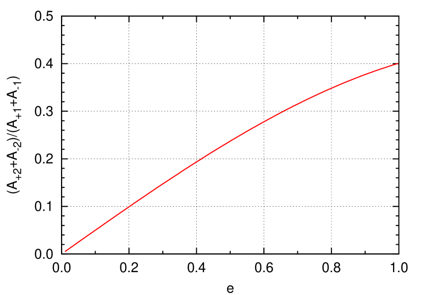
Figure 12: The expected amplitude ratio of the second sidelobes to the first sidelobes as a function of eccentricity $e$, in the case of $\varpi=0$ and $\alpha\ll 1$.

3.4.3 The case of $e\ll 1$

In the case of $e\ll 1$, as seen in equation (71), $(A_{+1}+A_{-1})/A_{0}\simeq\alpha\times(1+O(e^{2}))$. Hence, to the order of $O(e^{1})$, the eccentricity is determined by equation (76), and $\alpha$ is determined by

$$\alpha\simeq{{A_{+1}+A_{-1}}\over{A_{0}}}.$$ (79)

Similarly, within the same approximation, from equation (73),

$$\varpi\simeq{{\phi_{+1}-\phi_{-1}}\over{2}}.$$ (80)

As discussed in section 3.2.2, in the limit of $e\rightarrow 0$, $\varpi$ tends to $0$. Then, in this limit, $\phi_{+1}$ and $\phi_{-1}$ become equal each other, as expected from the analysis of circular orbits.

The mass function is given by

$$f(m_{1},m_{2},\sin i)=\left(\frac{A_{+1}+A_{-1}}{A_{0}}\right)^{3}\frac{P_{\rm osc}^{3}}{P_{\rm orb}^{2}}\frac{c^{3}}{2\pi G},$$ (81)

and $a_{1}\sin i$ is given by

$$a_{1}\sin i\simeq{{P_{\rm osc}}\over{2\pi}}{{A_{+1}+A_{-1}}\over{A_{0}}}c.$$ (82)

The radial velocity is obtained by setting $a_{1}(e)=b_{1}(e)=1$ and $a_{2}(e)=b_{2}(e)\simeq e/2$:

$$v_{\rm rad,1}(t) \simeq {{P_{\rm osc}}\over{P_{\rm orb}}}{{A_{+1}+A_{-1}}\over{A_{0}}}c$$ (83)

$$\times\left[(\cos\Omega t+e\cos 2\Omega t)\cos\left({{\phi_{+1}-\phi_{-1}}\over{2}}\right)\right.$$

$$-\left.(\sin\Omega t+e\sin 2\Omega t)\sin\left({{\phi_{+1}-\phi_{-1}}\over{2}}\right)\right].$$

3.5 Some more examples with artificial data

3.5.1 An example for the case of $\alpha\ll 1$

In order to see how the present method works, we generate artificial, noise-free light curve data. The input parameters are: $m_{1}=m_{2}=2$ M_⊙, $e=0.3$, $\varpi=0$, $i=90^{\circ}$, $\nu_{\rm osc}(\equiv 1/P_{\rm osc})=20$ d^-1 and $P_{\rm orb}=1$ d, giving $\alpha=1.13\times 10^{-2}$. This case could apply to a binary star with two $\delta$ Sct stars in an eccentric orbit. The infinite series of $a_{n}$ and $b_{n}$ were truncated at $N=150$.

The top panel of Fig. 13 shows the amplitude spectrum of the generated data sampled with 10 points per pulsation cycle over a time span of 10 orbital periods after the central peak of amplitude 1.0 (in intensity) has been prewhitened. There is no phase difference between the sidelobes. From this $\varpi=0$ is deduced. The first sidelobes have almost equal amplitudes of only $5.4\times 10^{-3}$ the amplitude of the central peak. This is consistent with equations (62) and (65). The second sidelobes also have almost equal amplitudes, and their amplitude ratio to the first sidelobes is 0.15, as expected from equation (76). Further sidelobes have such small amplitudes that they are unlikely to be observed in this case.

From the amplitude ratio of the second sidelobes to the first sidelobes, $0.15$, the value of eccentricity $e=0.30$ is reproduced well. Combining this with the amplitude ratio of the first sidelobes to the central peak, $0.0108$, we determine $\alpha$ and the mass function; $1.08\times 10^{-2}$ and $0.43\,{\rm M}_{\odot}$, respectively. These values determined from the amplitude spectrum are also in satisfactory agreement with the true values; $1.13\times 10^{-2}$ and $0.5\,{\rm M}_{\odot}$, respectively.

The bottom panel of Fig. 13 demonstrates how well the radial velocity curve is reproduced. The true radial velocity is shown with red, and the one determined from the amplitude spectrum is shown with green. The latter is the solution of $O(e^{1})$ obtained from equation (83). This is the crudest solution. The blue curve corresponds to the radial velocity curve that can ultimately be determined within this framework from equation (78) with a higher-order approximation. We see the radial velocity curve is reasonably well reproduced.

To summarise this experiment with artificial data: We conclude that in the case of $\alpha\ll 1$ the binary parameters are reproduced well from the photometric light curve alone.

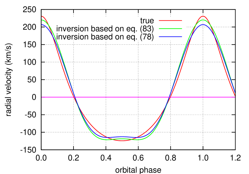
Figure 13: Top panel: An amplitude spectrum for artificial data with $m_{1}=m_{2}=2$ M_⊙, $e=0.3$, $\varpi=0$, $i=90^{\circ}$, $\nu_{\rm osc}=20$ d^-1 and $P_{\rm orb}=1$ d after prewhitening the central peak, which has an intensity amplitude of 1.0, by definition. Bottom panel: The true radial velocity curve (red) and two photometrically determined ones (green and blue). The green curve is obtained from the first and the second sidelobes and the central peak in the amplitude spectrum, based on equation (83); the blue curve is a solution based on equation (78). Note that they are obtained without iteration.

3.5.2 A more extreme case of $\alpha>1$

We now note that amplitude spectra are not so simple in all cases. Taking an extreme example, Fig. 14 shows a case where $\alpha=5.6$ that is equivalent to a 10-s pulsar in a 1-d binary with another neutron star. The parameters are: $m_{1}=m_{2}=3$ M_⊙, $e=0.3$, $\varpi=0$, $\nu_{\rm osc}=100$ mHz, $P_{\rm orb}=1$ d and $i=90^{\circ}$. Note that the central peak of the multiplet in this case has almost no amplitude, and that the pattern is highly asymmetric.

Figure 14: The amplitude spectrum for artificial data with $m_{1}=m_{2}=3$ M_⊙, $e=0.3$, $\varpi=0$, $i=90^{\circ}$, $\nu_{\rm osc}=100$ mHz ($P_{\rm osc}=10$ s) and $P_{\rm orb}=1$ d; $\alpha=5.6$. The amplitude scale is in fractional intensity.

3.6 An actual example, KIC 4150611 revisited

In section 2.6, we assumed that KIC 4150611 has a circular orbit. How is this assumption justified? In the case of an eccentric orbit, the amplitude ratio of the second sidelobes to the first sidelobes is proportional to $e$, as long as $\alpha\ll 1$. In the case of KIC 4150611, the multiplet is seen as a triplet, not a quintuplet. Hence, the eccentricity is smaller than the detection limit, and the assumption of a circular orbit adopted in section 2.6 is consistent with the observation.

From Table 3 we see that the root-mean-square error on amplitude is 0.007 mmag, hence at the 1$\sigma$ level an upper limit to the eccentricity can be made from the noise level for the quintuplet sidelobes. From equation (68) we then find $e\leq 0.12$ for the highest amplitude pulsation frequency. Hence at the 3$\sigma$ level the constraint on the eccentricity is weak. Supposing that the orbit of KIC 4150611 is non-circular, we estimate the angle $\varpi$ from the phase difference $(\phi_{+1}-\phi_{-1})/2$. This value is $-0.02\pm 0.04$ radians for the triplet of $\nu_{\rm osc}=22.619577$ d^-1. The estimated value of $\alpha$ is the same as that determined with the assumption of a circular orbit, thus the mass function is the same as that derived in section 2.6.

4 Exoplanet hunting

A new application of our method is in the search for exoplanets. The prime goal of the CoRoT and Kepler missions is to find exoplanets by the transit method. The other main technique for exoplanet searches is the radial velocity technique using high-resolution ground-based spectroscopy. Both of these techniques have concentrated on solar-like and lower main sequence stars where planetary transits are deeper than for hotter main sequence stars, and where radial velocities are greater than for more massive host stars. Now with our new technique of photometric measurement of radial velocity, there is a possibility to detect planets around hotter main sequence pulsating stars, such as $\delta$ Sct and $\beta$ Cep stars, and around compact pulsating stars, such as subdwarf B pulsators and various pulsating white dwarf stars. This has been demonstrated in the case of the subdwarf B pulsator V391 Peg (Silvotti et al., 2007) using the $O-C$ method.

Let us look here at the possibility of exoplanet detection using our method. It can be seen in equations (21) and (25) that the frequency triplet in the amplitude spectrum of a pulsating star with a planetary companion will have larger sidelobes for higher pulsation frequency and for longer orbital period. We therefore examine a limiting case for the Kepler mission of a 1.7-M_⊙ $\delta$ Sct star with a pulsation frequency of 50 d^-1 and with a planetary companion of one Jupiter mass ($10^{-3}$ M_⊙), with an orbital period of 300 d and an inclination of $i=90^{\circ}$. In this case $\alpha=1.1\times 10^{-3}$ is small.

We find that the first orbital sidelobes have amplitudes of $558\times 10^{-6}$ where the central peak has an amplitude of 1. With Kepler data we can reach photometric precision of a few $\mu$mag, so can detect signals of, say, 10 $\mu$mag and higher. This means that we need to have pulsation amplitudes of 0.02 mag, or more, to detect a Jupiter-mass planet with the orbital parameters given above. This is possible; there are, for example, $\delta$ Sct stars with amplitudes greater than 0.02 mag.

To take another case, can we detect a hot 10-M_Jupiter planet in a 10-d orbit around a $\delta$ Sct star? In this case $\alpha=1.2\times 10^{-3}$, so the detection limit is about the same as above: the sidelobes have amplitudes of $576\times 10^{-6}$ where the central peak has an amplitude of 1. Signals such as these should be searched for in High Amplitude $\delta$ Sct (HADS) stars. Compact stars also offer potential exoplanet discoveries with our technique.

Through photometric radial velocity measurement, the mass of the exoplanet can then be estimated with an assumption about the mass of the host star. If planetary transits are detected for the same exoplanet system, the size of the planet can also be derived. Hence the mean density of the exoplanet can be determined only through the photometric observations.

5 Discussion

5.1 Photometric radial velocity measurement

As clearly seen in equation (1), the phase of the luminosity variation of a pulsating star in a binary system has information about the radial velocity due to the orbital motion. By taking the time derivative of the phase of pulsation, we can obtain the radial velocity at each phase of the orbital motion. We have shown in this paper that the Fourier transform of the light curve of such a pulsating star leads to frequency multiplets in the amplitude spectra where the frequency splitting and the amplitudes and phases of the components of the frequency multiplet can be used to derive all of the information traditionally found from radial velocity curves.

This is a new way of measuring the radial velocity. Until now, to measure radial velocity we have had to carry out spectroscopic observations of the Doppler shift of spectral lines. In contrast, the present result means that radial velocity can be obtained from photometric observations alone. In the case of conventional ground-based observations, getting precise, uninterrupted measurements of luminosity variations is highly challenging at mmag precision. However, this situation has changed dramatically with space missions such as CoRoT and Kepler, which have $\mu$mag precision with duty cycles exceeding 90 per cent. Telescope time for spectroscopic observations is competitive, and suffers from most of the same ground-based limitations as photometry. Now for binary stars with pulsating components, a full orbital solution can be obtained from the light curves alone using the theory we have presented.

5.2 Limitations

There are clear limitations to the application of the theory presented here. Firstly, the pulsating stars to be studied must have stable pulsation frequencies. Many pulsating stars do not. In the Sun, for example, the pulsation frequencies vary with the solar cycle. That would not be much limitation for current Kepler data, since the solar cycle period is so long compared with the time span of the data. But other pulsating stars also show frequency variability, and on shorter time scales. RR Lyrae stars show the Blazhko effect, which has frequency, as well as amplitude variability. Other pulsating stars show frequency changes much larger than expected from evolution on time scales that are relevant here. Thus, to apply this new technique, a first step is to find pulsating stars with stable frequencies and binary companions. The best way to do this is to search for the frequency patterns we have illustrated in this work.

Another limitation can arise from amplitude modulation in a pulsating star. While this will not cause frequency shifts, it will generate a set of Fourier peaks in the amplitude spectrum that describe the amplitude modulation. For nonperiodic modulation on time scales comparable to the orbital period, the radial velocity sidelobe signal may be lost in the noise.

Of course, it is imperative when frequency triplets or multiplets are found to distinguish among rotational multiplets with $m$ modes, oblique pulsator multiplets that are pure amplitude modulation, and the frequency multiplets caused by frequency modulations. As we have explained in this paper, this can be done by careful examination of frequency separations, amplitudes and phases. For the latter, a correct choice of the time zero point is imperative.

The important characteristics of FM multiplets is that the amplitude ratio of the sidelobes to the central peak is the same for all pulsation frequencies, and (for low eccentricity systems) the phases of the sidelobes are in quadrature with that of the central peak at the time of zero radial velocity, e.g., the time of eclipse for $i=90^{\circ}$. We anticipate more of these stars being found and astrophysically exploited.

References

- Aerts et al. (2010) Aerts C., Christensen-Dalsgaard J., Kurtz D. W., 2010, Asteroseismology, Springer
- Anger (1855) Anger C. T., 1855, Neueste Schriften der Naturf. Ges. in Danzig, p.2
- Bailes et al. (1991) Bailes M., Lyne A. G., Shemar S. L., 1991, Nature, 352, 311
- Benkő et al. (2009) Benkő J. M., Paparó M., Szabó R., Chadid M., Kolenberg K., Poretti E., 2009, in American Institute of Physics Conference Series, Vol. 1170, American Institute of Physics Conference Series, J. A. Guzik & P. A. Bradley, ed., pp. 273–275
- Benkő et al. (2011) Benkő J. M., Szabó R., Paparó M., 2011, MNRAS, 417, 974
- Bernoulli (1738) Bernoulli D., 1738, Hydrodynamica
- Bigot & Kurtz (2011) Bigot L., Kurtz D. W., 2011, A&A, 536, A73
- Bloemen et al. (2011) Bloemen S., Marsh T. R., Østensen R. H., Charpinet S., Fontaine G., Degroote P., Heber U., Kawaler S. D., Aerts C., Green E. M., Telting J., Brassard P., Gänsicke B. T., Handler G., Kurtz D. W., Silvotti R., van Grootel V., Lindberg J. E., Pursimo T., Wilson P. A., Gilliland R. L., Kjeldsen H., Christensen-Dalsgaard J., Borucki W. J., Koch D., Jenkins J. M., Klaus T. C., 2011, MNRAS, 410, 1787
- Brouwer & Clemence (1961) Brouwer D., Clemence G. M., 1961, Methods of celestial mechanics, New York: Academic Press
- Cayley (1861) Cayley A., 1861, Mem. Roy. Astron. Soc., 29, 191
- Hulse & Taylor (1975) Hulse R. A., Taylor J. H., 1975, ApJ, 195, L51
- Jacobi (1836) Jacobi C. G. J., 1836, Journal für Math., xv, p.12
- Koch et al. (2010) Koch D. G., Borucki W. J., Basri G., Batalha N. M., Brown T. M., Caldwell D., Christensen-Dalsgaard J., Cochran W. D., DeVore E., Dunham E. W., Gautier III T. N., Geary J. C., Gilliland R. L., Gould A., Jenkins J., Kondo Y., Latham D. W., Lissauer J. J., Marcy G., Monet D., Sasselov D., Boss A., Brownlee D., Caldwell J., Dupree A. K., Howell S. B., Kjeldsen H., Meibom S., Morrison D., Owen T., Reitsema H., Tarter J., Bryson S. T., Dotson J. L., Gazis P., Haas M. R., Kolodziejczak J., Rowe J. F., Van Cleve J. E., Allen C., Chandrasekaran H., Clarke B. D., Li J., Quintana E. V., Tenenbaum P., Twicken J. D., Wu H., 2010, ApJ, 713, L79
- Kurtz (1982) Kurtz D. W., 1982, MNRAS, 200, 807
- Lebrun (1977) Lebrun M., 1977, Computer Music J., 1(4), 1
- Ledoux (1951) Ledoux P., 1951, ApJ, 114, 373
- Legendre (1769) Legendre A.-M., 1769, Hist. de l’Acad. R. des Sci. de Berlin, 204
- Shibahashi & Takata (1993) Shibahashi H., Takata M., 1993, PASJ, 45, 617
- Silvotti et al. (2007) Silvotti R., Schuh S., Janulis R., Solheim J.-E., Bernabei S., Østensen R., Oswalt T. D., Bruni I., Gualandi R., Bonanno A., Vauclair G., Reed M., Chen C.-W., Leibowitz E., Paparo M., Baran A., Charpinet S., Dolez N., Kawaler S., Kurtz D., Moskalik P., Riddle R., Zola S., 2007, Nature, 449, 189
- Sterken (2005) Sterken C., 2005, in Astronomical Society of the Pacific Conference Series, Vol. 335, The Light-Time Effect in Astrophysics: Causes and cures of the O-C diagram, C. Sterken, ed., p. 215
- Unno et al. (1989) Unno W., Osaki Y., Ando H., Saio H., Shibahashi H., 1989, Nonradial oscillations of stars, Tokyo: University of Tokyo Press, 1989, 2nd ed.
- Watson (1922) Watson G. N., 1922, A treatise on the theory of Bessel functions, Cambridge University Press, Cambridge
- Wolszczan & Frail (1992) Wolszczan A., Frail D. A., 1992, Nature, 355, 145