Opportunistic Scheduling in Heterogeneous Networks: Distributed Algorithms and System Capacity

Abstract

In this work, we design and analyze novel distributed scheduling algorithms for multi-user MIMO systems. In particular, we consider algorithms which do not require sending channel state information to a central processing unit, nor do they require communication between the users themselves, yet, we prove their performance closely approximates that of a centrally-controlled system, which is able to schedule the strongest user in each time-slot.

Our analysis is based on a novel application of the Point-Process approximation. This novel technique allows us to examine non-homogeneous cases, such as non-identically distributed users, or handling various QoS considerations, and give exact expressions for the capacity of the system under these schemes, solving analytically problems which to date had been open. Possible application include, but are not limited to, modern 4G networks such as 3GPP LTE, or random access protocols.

1 Introduction

Consider the problem of scheduling users in a multi-user MIMO system. For several decades, at the heart of such systems stood a basic division principle: either through TDMA, FDMA or more complex schemes, users did not use the medium jointly, but rather used some scheduling mechanism to ensure only a single user is active at any given time. Numerous medium access (MAC) schemes at the data link layer also, in a sense, fall under this category. Modern multi-user schemes, such as practical multiple access channel codes or dirty paper coding (DPC) for Gaussian broadcast channels [1], do allow concurrent use of a shared medium, yet, to date, are complex to implement in their full generality. As a result, even modern 4G networks consider scheduling groups of users, each of which employing a complex multi-user code [2, 3].

Hence, scheduled designs, in which only a single user or a group of users utilize the medium at any given time, are favorable in numerous practical situations. In these cases, the goal is to design an efficient schedule protocol, and compute the resulting system capacity. In this work, we derive the capacity of multi-users MIMO systems under distributed scheduling algorithms, in which each user experiences a different channel distribution, subject to various QoS considerations.

1.1 Related Work

Various suggested protocols in the current literature follow the pioneering work of [4]. In these systems, at the beginning of a time-slot, a user computes the key parameters relevant for that time-slot. For example, the channel matrix $\mathbf{H}$ (Figure 1). It then sends these parameters to a central processing unit, which decides which user to schedule for that time-slot. This enables the central unit to optimize some criterion, e.g., the number of bits transmitted in each slot, by scheduling the user with the best channel matrix. This is the essence of multi-user diversity. In [5], the authors adopted a zero-forcing beamforming strategy, where users are selected to reduce the mutual interference. The scheme was shown to asymptotically achieve the performance of DPC. An enhanced cooperative scheme, in which base stations optimize their beamforming coordination, such that the users' transmitting power is subject to SINR minmax fairness, is given in [6]. Its analysis showed that optimal beamforming strategies have an equivalent convex optimization problem. Yet, its solution requires centralized CSI knowledge. In [7], the authors devised a multi-user diversity with interference avoidance by mitigation approaches, which selects the user with the highest minimal eigenvalue of his Wishart channel matrix $\textbf{H}\textbf{H}^{\dagger}$. [8] proposed a scheduling scheme that transmit only to a small subset of heterogeneous users with favorable channel characteristics. This provided near-optimal performance when the total number of users to choose from was large. Scaling laws for the sum-rate capacity comparing maximal user scheduling, DPC and BF were given in [9]. Additional surveys can be found in [10, 11]. Subsequently, [12] analyzed the scaling laws of maximal base station scheduling via Extreme Value Theory (EVT), and showed that by scheduling the station with the strongest channel among $K$ stations (Figure 1), one can gain a factor of $O(\sqrt{2\log K})$ in the expected capacity compared to random or Round-Robin scheduling.

Extreme value theory and order statistics are indeed the key methods in analyzing the capacity of such scheduled systems. In [13], the authors suggested a subcarrier assignment algorithm (in OFDM-based systems), and used order statistics to derive an expression for the resulting link outage probability. Order statistics is required, as one wishes to get a handle on the distribution of the selected users, rather than the a-priori distribution. In [14], the authors used EVT to derive throughput and scaling laws for scheduling systems using beamforming and various linear combining techniques. [15] discussed various user selection methods in several MIMO detection schemes. The paper further strengthened the fact that appropriate user selection is essential, and in several cases can even achieve optimality with sub-optimal detectors. Additional user-selection works can be found in [16, 17, 18, 19].

In [20, 21], the authors suggested a decentralized MAC protocol for OFDMA channels, where each user estimates his channels gain and compares it to a threshold. The optimal threshold is achieved when only one user exceeds the threshold on average. This distributed scheme achieves $1/e$ of the capacity which could have been achieved by scheduling the strongest user. The loss is due to the channel contention inherent in the ALOHA protocol. [22] extended the distributed threshold scheme for multi-channel setup, where each user competes on $m$ channels. In [23] the authors used a similar approach for power allocation in the multi-channel setup, and suggested an algorithm that asymptotically achieves the optimal water filling solution. To reduce the channel contention, [20, 24] introduced a splitting algorithm which resolves collision by allocating several mini-slots devoted to finding the best user. Assuming all users are equipped with a collision detection (CD) mechanism, the authors also analyzed the suggested protocol for users that are not fully backlogged, where the packets randomly arrive with a total arrival rate $\lambda$ and for channels with memory. [25] used a similar splitting approach to exploit idle channels in a multichannel setup, and showed improvement of $63\%$ compared to the original scheme in [20].

1.2 Main Contribution

In this work, we suggest a novel technique, based on the Point Process approximation, to analyze the expected capacity of scheduled multi-user MIMO systems. We first briefly show how this approximation allows us to derive recent results described above. However, the strength of this approximation is in facilitating the asymptotic (in the number of users) analysis of the capacity of such systems in different non-uniform scenarios, where users are either inherently non-uniform or a forced to act this way due to Quality of Service constrains. We compute the asymptotic capacity for non-uniform users, when users have un-equal shares or when fairness considerations are added. To date, these scenarios did not yield to rigorous analysis.

Furthermore, we suggest a novel distributed algorithm, which achieves a constant factor of the maximal multi-user diversity without centralized processing or communication among the users. Moreover, we offer a collision avoidance enhancement to our algorithm, which asymptotically achieves the maximal multi-user diversity without any collision detection mechanism.

The rest of this paper in organized as follows. In Section 2, we describe the system model and related results. In Section 3, we describe the Point of Process technique and briefly show how it is utilized. In Section 4 we analyze the non-uniform scenario. In Section 5 we examine the expected capacity in a non-uniform environment, assuming that the receiver can recover the message from a single collision. In Section 6 we describe the distributed algorithm and analyze its performance. Section 7 concludes the paper.

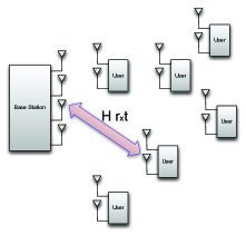
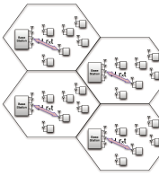
Figure 1: (a) Multi-user MIMO. (b) MU-MIMO stations.

2 Preliminaries

We consider a multiple-access model with $K$ users. The channel model is the following:

$$\textbf{y}=\textbf{H}x+\textbf{n}$$

where $\textbf{y}\in\mathbb{C}^{r}$ is the received vector and $r$ is the number of receiving antennas. $x\in\mathbb{C}^{t}$ is the transmitted vector constrained in its total power to $P$, i.e., $E[x^{\dagger}x]\leq P$, where $t$ is the number of transmitting antennas. $\textbf{H}\in\mathbb{C}^{r\times t}$ is a complex random Gaussian channel matrix such that all the entries are random $i.i.d.$ complex Gaussian with independent imaginary and real parts, zero mean and variance $1/2$ each. $\textbf{n}\in\mathbb{C}^{r}$ is uncorrelated complex Gaussian noise with independent real and imaginary parts, zero mean and variance 1. In the MIMO uplink model, we assume that the channel H is known at the transmitters. In the centralized scheme, the transmitters send their channel statistics to the receiver. I.e., the channel output at the receiver consist of the pair $(\textbf{y},\textbf{H})$. Then, the receiver lets to the transmitter with the strongest channel to transmit in the next slot. In the MIMO downlink model, we assume that the channel H is known at the receivers. In the centralized scheme, the receivers send their channel statistics to the transmitter, so he can choose the receiver that will benefit most from his transmission. Moreover, we assume that the channel is memoryless, such that for each channel use, an independent realization of H is drawn. Through this paper, we use bold face notation for random variables.

2.1 MIMO Capacity

[26, 27] and [28] show that when the elements of the channel gain matrix, H, are i.i.d. zero mean with finite moments up to order $4+\delta$, for some $\delta>0$ then the distribution of the capacity follows the Gaussian distribution by the CLT, as we can see in Figure 2, with mean that grows linearly with $min(r,t)$, and variance which is mainly influenced by the power constraint $P$.

With the observation that the channel capacity follows the Gaussian distribution, we would first like to investigate the extreme value distribution that the capacity follows, and thus retrieve the capacity gain when letting a user with the best channel statistics among all other users, utilize a slot.

2.2 Extreme Value Analysis for the Maximal Value

In this sub-section we review the Extreme Value Theorem (EVT), from [29],[30] and [31], that will later be used for asymptotic capacity gain analysis.

Theorem 1 ([32, 29, 31]).

1. Suppose that $\textbf{x}_{1},..\textbf{x}_{n}$ is a sequence of $i.i.d$ random variables with distribution function $F(x)$, and let

   $$M_{n}=\max(\textbf{x}_{1},...,\textbf{x}_{n}).$$

   If there exist a sequence of normalizing constants $a_{n}>0$ and $b_{n}$ such that as $n\rightarrow\infty$,

   $$\Pr(M_{n}\leq a_{n}x+b_{n})\stackrel{{\scriptstyle i.d.}}{{\longrightarrow}}G(x)$$ (1)

   for some non-degenerate distribution G, then G is of the generalized extreme value (GEV) distribution type

   $$G(x)=\exp\left\{-(1+\xi x)^{-1/\xi}\right\}$$ (2)

   and we say that $F(x)$ is in the domain of attraction of $G$, where $\xi$ is the shape parameter, determined by the ancestor distribution $F(x)$ with the following relation.

2. Let $h$ be the following reciprocal hazard function

   $$h(x)=\frac{1-F(x)}{f(x)}\textmd{ for }x_{F}\leq x\leq x^{F},$$ (3)

   where $x_{F}=inf\{x:F(x)>0\}$ and $x^{F}=sup\{x:F(x)<1\}$ are the lower and upper endpoints of the ancestor distribution, respectively. Then the shape parameter $\xi$ is obtained as the following limit,

   $$\frac{d}{dx}h(x)\stackrel{{\scriptstyle x\rightarrow x^{F}}}{{\longrightarrow}}\xi.$$ (4)

3. If $\{\textbf{x}_{n}\}$ is an i.i.d. standard normal sequence of random variables, then the asymptotic distribution of $M_{n}=\max(\textbf{x}_{1},...\textbf{x}_{n})$ is a Gumbel distribution. Specifically,

   $$\Pr(M_{n}\leq a_{n}x+b_{n})\longrightarrow e^{-e^{-x}}$$

   where

   $$a_{n}=(2\log n)^{-1/2}$$ (5)

   and

   $$b_{n}=(2\log n)^{1/2}-\frac{1}{2}(2\log n)^{-1/2}(\log\log n+\log 4\pi).$$ (6)

In Figure 3 we see the max value distribution for $500$ observations which following the Gaussian distributed simulated in Figure 2 For completeness, a sketch of the proof is given in Appendix A. Similarly, if $\{\textbf{x}_{n}\}$ follows the Gaussian distribution with mean $\mu$ and variance $\sigma^{2}$, then the above theorem normalizing constants results in

$$a_{n}=\sigma(2\log n)^{-\frac{1}{2}}$$ (7)

and

$$b_{n}=\sigma\left[(2\log n)^{\frac{1}{2}}-\frac{1}{2}(2\log n)^{-\frac{1}{2}}[\log\log n+\log(4\pi)]\right]+\mu.$$ (8)

It follows that for a Gaussian distribution,

$$a_{n}=\sigma(2\log n)^{-\frac{1}{2}}\rightarrow 0,$$

which implies that

$$M_{n}\sim b_{n}\sim\sigma(2\log n)^{\frac{1}{2}}+\mu.$$ (9)

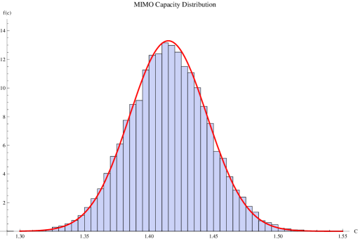
Figure 2: MIMO capacity distribution for m=32 transmitting antennas and n=128 receiving antennas vs. Gaussian Distribution with $\mu=\sqrt{2}$ and $\sigma=0.03$ (red line).

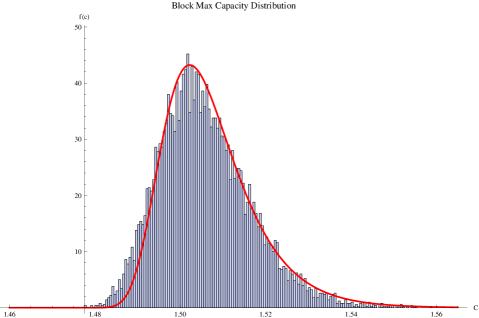
Figure 3: Maximal capacity distribution, when choosing the maximal capacity among 500 capacities that following the Gaussian distribution simulated in Figure 2, with $\mu=\sqrt{2}$ and $\sigma=0.03$. The red line is the corresponding Gumbel density plotted in range $[\mu+2\sigma,\mu+5\sigma].$

2.3 Multi-User Diversity

Assuming MIMO uplink model, i.e., perfect CSI of $K$ users at the receiver, then the expected capacity that we achieve by choosing the maximal user in each time slot will follow the expected value of Gumbel distribution with parameters $a_{K},b_{K}$ [12], i.e.,

$$E[M_{K}] \stackrel{{\scriptstyle(a)}}{{=}} \sigma\left(b_{K}+a_{K}\gamma\right)+\mu$$

$$\stackrel{{\scriptstyle(b)}}{{=}} \sigma\left[(2\log K)^{\frac{1}{2}}-\frac{1}{2}(2\log K)^{-\frac{1}{2}}[\log\log K+\log(4\pi)]+\gamma(2\log K)^{-\frac{1}{2}}\right]+\mu$$

where $\gamma\approx 0.57721$ is Euler-Mascheroni constant, $(a)$ follows from the expectation of the Gumbel distribution and $(b)$ follows from (5) and (6). Hence, for large enough $K$,

$$E[M_{K}]=\sigma(2\log K)^{\frac{1}{2}}+\mu+o\left(\frac{1}{\sqrt{\log K}}\right)$$

That is, for large number of users, the expectation capacity grows like $\sqrt{2\log K}$.

3 Distributed Algorithm

A major drawback of the previous method is that a base station must receive a perfect CSI from all users in order to decide which user is adequate to utilize the next time slot, which may not be feasible for a large number of users. Moreover, the delay caused by transmitting CSI to the base station would limit the performance.

In this section, we begin our discussion from a distributed algorithm, shown in [22], in which stations do not send their channel statistics to the base station, yet, with some subtle enhancements, the performance is asymptotically equal to that in (2.3). We provide an alternative analysis to this algorithm, that will serve us later in this paper.

The algorithm is as follows. Given the number of users, we set a high capacity threshold such that only a small fraction of the users will exceed it. In each slot, the users estimate their own capacity. If the capacity seen by a user is greater than the capacity threshold, he transmits in that slot. Otherwise, the user keeps silent in that slot. The base station can successfully receive the transmission if no collision occurs.

Let $C_{av}\left(u_{k}\right)$ denote the expected capacity, given a threshold $u_{k}$ such that $k\ll K$ i.i.d. users exceed it on average. For sufficiently large number of users, $K$, we obtain the following.

Proposition 1.

The expected capacity when working with a single user in each slot is

$$C_{av}\left(u_{k}\right) = ke^{-k}\left(u_{k}+\sigma a_{K}\right)+o(a_{K})$$ (11)

where $a_{K}$ is the normalizing constant given in (5).

Due to the distributed nature of the algorithm, some slots will be idle if no user exceeds the threshold, that is, no user transmits in that slot. Or, collisions may occur if more than one user exceed the threshold, that is, more than one user is trying to transmit in a slot. Thus, we say that a slot is utilized if exactly one user exceeds the threshold, namely, exactly one user transmits in a slot. Indeed, the expected capacity $C_{av}\left(u_{k}\right)$ has the form

$$C_{av}\left(u_{k}\right)=\Pr\left(\textmd{utilized slot}\right)E[C|C>u_{k}]$$

where

$$\Pr\left(\textmd{utilized slot}\right)=ke^{-k}$$ (12)

and

$$E[C|C>u_{k}]=u_{k}+a_{K}+o(a_{K}).$$ (13)

That is, to compute $C_{av}\left(u_{k}\right)$ we analyze the expected capacity when letting a user with above-threshold-capacity utilize a slot, and the probability that only a single user utilizes the slot. We choose to prove the above through the point process method [31, 33]. With the point of process, we can model and analyze the occurrence of large capacities, which can be represented as a point process, when considering the users index along with the capacity value. Later, in the main contribution of this paper, this method will allow us to analyze the non-uniform case as well.

The following two subsections sketch the key steps to prove Proposition 1. The first discusses the estimation of the threshold, given the fraction of users which are required to pass it on average. The second computes the distribution of the capacity, given that the threshold was passed. The third subsection discusses the rate at which users pass the threshold.

3.1 Threshold Estimation

Let $u_{k}$ be a threshold such that only $k$ strongest users will exceed that threshold. Assuming that the capacity follows a Gaussian distribution $\Phi(x)$, with mean $\mu$ and variance $\sigma^{2}$, $u_{k}$ can be easily estimated using the inverse error function.

Claim 1.

The threshold $u_{k}$, such that $k$ users out of total $K$ users will exceed it on average is

$$u_{k}=\mu+\sigma\sqrt{2\log\left(\frac{K}{k}\right)-\log\left[-2\pi\left(2\log\left(\frac{k}{K}\right)+\log[2\pi]\right)\right]}+o\left(K^{-2}\right)$$ (14)

Proof.

Let $\operatorname{erfc}^{-1}(\cdot)$ denote the complementary inverse error function. The threshold $u_{k}$ such that $1-\Phi(u_{k})=\frac{k}{K}$ is given by

$$u_{k} = \mu+\sqrt{2}\sigma\operatorname{erfc}^{-1}\left(\frac{2k}{K}\right)$$

$$= \mu+\sigma\sqrt{2\log\left(\frac{K}{k}\right)-\log\left[-2\pi\left(2\log\left(\frac{k}{K}\right)+\log[2\pi]\right)\right]}+o\left(K^{-2}\right).$$

where the last equality follows from a Taylor series expansion. ∎

Nevertheless, using the stability law of extreme values [30], the threshold can also be approximated for a large number of users directly. Indeed, using EVT, the threshold can be computed without evaluation of the inverse $\operatorname{erfc}(\cdot)$, which cannot be evaluated in closed form. On the other hand, the EVT relies itself on approximation. To gain sufficient amount of statistics, we logically divide the $K$ users to $\sqrt{K}$ blocks such that in each block there are $\sqrt{K}$ users, as we see in Figure 4. From the stability law of extreme values, the maximum in each block is still well approximated by GEV distributions. Thus, a threshold $u_{p}$, such that only a fraction $p=\frac{k}{\sqrt{K}}$ among $\sqrt{K}$ maximal users will exceed the threshold on average, attained as follows.

Claim 2.

The threshold $u_{p}$, such that $k$ strongest users out of total $\sqrt{K}$ strongest users will exceed it on average follows

$$u_{p} = \mu+\sigma\left(2\log\frac{\sqrt{K}}{k}\right)^{\frac{1}{2}}-\sigma\left(2\log\frac{\sqrt{K}}{k}\right)^{-\frac{1}{2}}\log\left\{-\log\left(1-\frac{k}{\sqrt{K}}\right)\right\}$$

$$+o\left(\frac{1}{\sqrt{(\log\frac{\sqrt{K}}{k})}}\right).$$

Proof.

An estimated threshold can be obtained by using EVT. A user estimates a threshold $u_{p}$ that is near $x^{F}$ such that only a fraction $p$ of the largest maximal capacities, among all maximal capacities, will exceed. For all $x$ that satisfies $a_{{p}^{-1}}x+b_{{p}^{-1}}>u_{p}$, i.e. are in the tail corresponding to the upper tail of Gumbel distribution, the return level $u_{p}$ is the $1-{p}$ quantile of the Gumbel distribution for all $0<p<1$, and has return period of $n={p}^{-1}$ observations. Thus, a user estimates the threshold by a simple quantile function,

$$1-G_{0}(u_{p})={p}.$$

For such $u_{p}$ we have

$$G(u_{p})=\exp\{-e^{-(u_{p}-b_{{p}^{-1}})/a_{{p}^{-1}}}\}=1-{p}$$ (16)

and we obtain that

$$u_{p}=b_{{p}^{-1}}-a_{{p}^{-1}}\log\left\{-\log(1-{p})\right\}+o(a_{{p}^{-1}}).$$ (17)

The $o(a_{{p}^{-1}})$ error is derived from the Gumbel approximation error, as shown in Appendix A . ∎

Note that the limit between $u_{p}$ given in (17) and $u_{k}$ given in (3.1) is $\frac{u_{p}}{u_{k}}\rightarrow\frac{3}{2\sqrt{2}}\approx 1.06$.

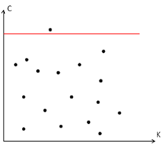
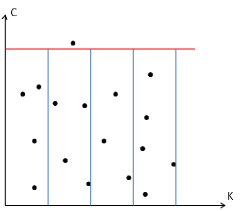
Figure 4: (a) $k=1$ users exceed a threshold out of $K$ observations. (b) Partitioning to $\sqrt{K}$ bins, such that in each bin there is approximately $\sqrt{K}$ users, and among this maximal users we set a threshold such that on average only the largest $k$ maximal users will exceed that threshold.

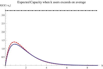
Figure 5: Threshold algorithm expected capacity gain for $K=1000$ users, when setting threshold such that $k$ users exceed on average by (3.1)(solid line) and by (17) (dashed line), comparing to the expected capacity of the optimal multi-user diversity centralized scheme (dot-dashed line).

In [20, Proposition 4] it is shown that the optimal threshold (maximum throughput) is obtained by demanding that only one user exceeds on average. This is also clear from Figure 5, for both threshold estimators.

3.2 Threshold Arrival Rate Point Process Approximation

In this section we discusses the rate at which users pass the threshold. That is, for a given threshold, we examine the average number of users that exceed the threshold in a single slot.

Assume that $\textbf{x}_{1},...,\textbf{x}_{n}$ is a sequence of $i.i.d$ random variables with a distribution function $F(x)$, such that $F(x)$ is in the domain of attraction of some GEV distribution G, with normalizing constants $a_{n}$ and $b_{n}$.
We construct a sequence of points $P_{1},P_{2},...$ on $[0,1]\times\mathbb{R}$ by

$$P_{n}=\left\{\left(\frac{i}{n},\frac{\textbf{x}_{i}-b_{n}}{a_{n}}\right),i=1,2,...,n\right\},$$

and examine the limit process, as $n\rightarrow\infty$.

Notice that the numbers of occurrences counted in disjoint intervals are independent from each other, and large points of the process are retained in the limit process, whereas all points $x_{i}=o(b_{n})$ can be normalized to same floor value $b_{l}$.

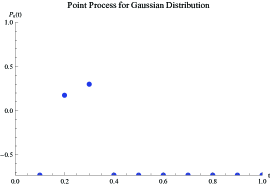
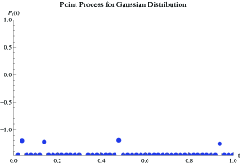
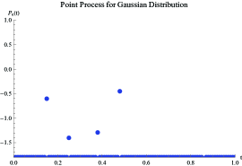
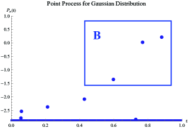
Figure 6: Point process for Gaussian distribution with $K\in\{10,50,100,1000\}$ users, in which all samples are normalized with $a_{K},b_{K}$ constants. As we can see, in each of process, only a small fraction of users are above the threshold. In particular, we obtain the expected number of arrivals to set $B$ by using (18).

Theorem 2 ([34, 33, 31]).

Consider $P_{n}$ on the set $[0,1]\times(b_{l}+\epsilon,\infty)$, where $\epsilon>0$, then

$$P_{n}\longrightarrow P\textmd{ as }n\rightarrow\infty$$

where $P$ is a non-homogeneous Poisson process with intensity density

$$\lambda(t,x)=(1+\xi x)_{+}^{-\frac{1}{\xi}-1}$$

where $x$ is the sample value, and $t$ is the index of occurrence.

In the case where all the users are i.i.d., the process intensity density $\lambda(t,x)$ is independent in the index of occurrence $t$. For completeness, a proof in Appendix B.
Let $\Lambda(B)$ be the expected number of points in the set $B$. $\Lambda(B)$ can be obtained by integrating the intensity of the Poisson process over $B$, That is

$$\Lambda(B)=\int_{b\in B}{\lambda(b)db}.$$ (18)

In this paper we are mainly interested in sets of the form

$$B_{v}=[0,1]\times(v,\infty)$$

where $v>b_{l}$. In this case

$$\Lambda(B_{v}) = \Lambda([0,1]\times(v,\infty))$$

$$= \int_{t=0}^{1}\int_{x=v}^{\infty}\lambda(t,x)dxdt$$

$$= \int_{t=0}^{1}\left[-(1+\xi x)_{+}^{-1/\xi}\right]_{x=v}^{\infty}$$

$$= \int_{t=0}^{1}\left(1+\xi v\right)_{+}^{-1/\xi}dt$$

$$= (1+\xi v)_{+}^{-1/\xi}$$

where $a_{+}$ denotes $\max\{0,a\}$.

That is, occurrences of above threshold capacities can be modeled by a Poisson process, with parameter $\Lambda\left(B_{v}\right)$. Namely, users normalized capacities exceed the threshold $v$ continuously and independently at a constant average rate $\Lambda(B_{v})$. In Figure 6-6 we observe the convergence of the point process to a continues process, that is, the Poisson process. This enables us to examine important events, e.g., how likely it is to have several threshold exceedances, or what is the expected distance that users reach from the threshold. Thus, analyze the expected capacity.

3.3 Tail Distribution

Focusing on points of the process $P_{n}$ that are above a threshold, we wish to examine the distribution of the distance that they reached from the threshold, that is the excess capacity above the threshold.

For any fixed $v>b_{l}$ let

$$u(v)=a_{n}v+b_{n},$$

and let $x>0$, then

$$\Pr\left(\textbf{x}_{i}>a_{n}x+u(v)|\textbf{x}_{i}>u(v)\right) = \Pr\left(\frac{\textbf{x}_{i}-b_{n}}{a_{n}}>x+v|\frac{\textbf{x}_{i}-b_{n}}{a_{n}}>v\right)$$

$$= \Pr(P_{n}(t)>x+v|P_{n}(t)>v)$$

$$\rightarrow \Pr(P(t)>x+v|P(t)>v)$$

where $P_{n}(t)$ and $P(t)$ are the corresponding excess value $\frac{\textbf{x}_{i}-b_{n}}{a_{n}}$ at index $t$, and the corresponding excess value at time $t$ in the limit process, respectively. The last step is obtained from the convergence in distribution shown in Theorem 2. Now,

$$\Pr(P(t)>x+v|P(t)>v) = \frac{\Lambda(B_{x+v})}{\Lambda(B_{v})}$$

$$= \left[\left(1+\xi\frac{x}{1+\xi v}\right)_{+}\right]^{-1/\xi}$$

$$= \left[\left(1+\xi\frac{x}{\sigma_{v}}\right)_{+}\right]^{-1/\xi}$$

where $\sigma_{v}=1+\xi v$. Hence, the limiting distribution for large threshold

$$\Pr\left(\textbf{x}_{i}>u(v)+a_{n}x|\textbf{x}_{i}>u(v)\right)$$

follows generalized Pareto distribution, $GPD(a_{n}\sigma_{v},\xi)$.

Note that for the Gaussian case $\xi\rightarrow 0$, and (3.3) reduces to

$$\Pr(\textbf{x}-u(v)\leq\alpha|\textbf{x}-u(v)>0)=1-e^{-\frac{\alpha}{a_{n}}}$$ (20)

for all $\alpha\geq 0$.

Thus, the Gaussian distribution tail is well approximated by an exponential distribution with rate parameter $\lambda=1/a_{n}$, as shown in Figure 7. As a result, by taking expected value on the capacity tail distribution we obtain the corollary, which is exactly (13).

Corollary 1.

The expected capacity seen by a user who passed the threshold $u_{k}$, where $k$ is the expected number of users to exceed $u_{k}$ out of $K$ users, is

$$E[\mathcal{C}|\mathcal{C}>u_{k}] = u_{k}+a_{K}+o\left(a_{K}\right).$$

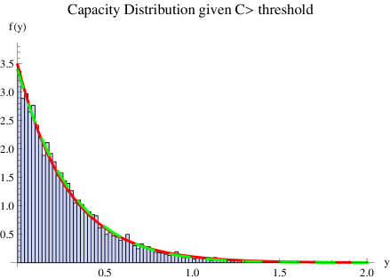
Figure 7: Tail of Gaussian distribution, statistics of 11722 observation out of 50000000 that exceed threshold 3.5, which is $\approx 1-\Phi(3.5)$ of the observations. Dashed line is obtained by analyzing conditional distribution of Gaussian capacity given that capacity is above threshold. the solid line obtained from (20). In both the threshold was derived from (17) ,

3.4 Throughput Analysis

As mentioned, we say that a slot is utilized only if a single user transmits in that slot. If more than one user exceeds the threshold in a slot, or no user exceeds the threshold in a slot, then the whole slot is lost. To address these scenarios we will offer a subtle collision avoidance algorithm in the following section. Using the point process method those events are very easy to analyze as we see in Figure 8 and Figure 8.

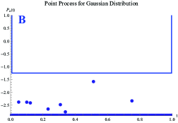
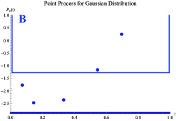
Figure 8: (a) Idle slot in point process point of view. (b) Collision slot in point process point of view.

Claim 3.

For a threshold $u_{k}$ we have:

$$\Pr\left(\textmd{ utilized slot }\right) = ke^{-k}.$$ (21)

Proof.

The probability that more than two out of $K$ users will exceed $u_{k}$ follows

$$\Pr(\textmd{ collision }) = \sum_{j=2}^{K}\binom{K}{j}\left(1-\Phi(u_{k})\right)^{j}\left(\Phi(u_{k})\right)^{K-j}$$

$$= 1-\left[\left(1-\frac{k}{K}\right)^{K}+K\left(\frac{k}{K}\right)\left(1-\frac{k}{K}\right)^{K-1}\right]$$

$$\stackrel{{\scriptstyle K\rightarrow\infty}}{{\longrightarrow}} 1-e^{-k}(k+1).$$

This also implies that the number of users exceeding the threshold follows the Binomial distribution with parameters $B(K,\frac{k}{K})$, hence, converges towards the Poisson distribution as $K$ goes to infinity.

Similarly, under the same settings, the probability of an idle slot is

$$\Pr\left\{\textmd{ idle slot }\right\} = \left(1-\frac{k}{K}\right)^{K}$$

$$\stackrel{{\scriptstyle K\rightarrow\infty}}{{\longrightarrow}} e^{-k}.$$

Since

$$\Pr\left(\textmd{ utilized slot }\right)=1-\Pr\left(\textmd{ idle slot }\bigcup\textmd{ collision }\right)$$

Claim 3 follows. ∎

In particular, (3.4) implies that the system will be idle $e^{-1}$ of the time when setting the optimal threshold, which is a threshold such that a single user exceeds the threshold on average [20, Proposition 4].

Proposition 1 now follows from Claim 3 and Corollary 1.

Remark.

It is interesting to see that the GEV distribution given in equation (2) can be derived from the Point process approximation we use in this paper.

To see this, set a threshold $u$, and for each random variable $\textbf{x}_{i}$ define

$$\textbf{y}_{i}=\mathbbm{1}_{\left\{\frac{\textbf{x}_{i}-b_{n}}{a_{n}}>u\right\}},$$

where $\mathbbm{1}_{\{\cdot\}}$ is the indicator function. We have

$$\lim_{n\to\infty}\Pr\left\{\max_{i}\textbf{x}_{i}\leq a_{n}u+b_{n}\right\} = \lim_{n\to\infty}\Pr\left\{\frac{\textbf{x}_{i}-b_{n}}{a_{n}}\leq u\textmd{ for all }i\right\}$$

$$= \lim_{n\to\infty}\Pr\left\{\sum_{i}\textbf{y}_{i}=0\right\}$$

$$= \exp\left\{-\Lambda(B_{u})\right\}$$

$$= \exp\left\{-\left(1+\xi u\right)^{-1/\xi}\right\}.$$

The $r-largest$ users can be obtained in a similar way.

4 Heterogeneous Users

We are now ready to address the main problem in this work. Specifically, in this section we assume that each user may be located at a different location, experiencing attenuation, delay and phase shift with different statistics compared to other users. In our setting, the different statistics are reflected in different mean and variance of the capacity. Since users are now non-uniform, previous methods of EVT, e.g. those used in [12], do not apply directly. However, using the Point of Process approximation derived in the previous section with subtle modification, enable us to analyze this model and the distributed threshold scheme.

From now on, we assume the $i$-th user capacity follows a Gaussian distribution with mean $\mu_{i}$ and variance $\sigma_{i}^{2}$. Let $C_{av}^{nu}(u)$ denote the expected capacity in this non-uniform environment. Our main result is the following.

Theorem 3.

The expected capacity when working with a single user in each slot in the above non-uniform environment, where the $i_{th}$ user capacity is approximated with mean $\mu_{i}$ and variance $\sigma^{2}_{i}$, follows

$$C_{av}^{nu}(u)=\frac{1}{K}\Lambda_{T}e^{-\frac{1}{K}\Lambda_{T}}\sum_{i=1}^{K}\frac{\Lambda_{i}}{\Lambda_{T}}\left(u+\sigma_{i}a_{K}+o(a_{K})\right)$$

where

$$\Lambda_{i}=e^{-\frac{u-(\sigma_{i}b_{K}+\mu_{i})}{\sigma_{i}a_{K}}}$$ (24)

is the average threshold exceedance rate of the $i_{th}$ user, and

$$\Lambda_{T}=\sum_{i=1}^{K}\Lambda_{i}$$ (25)

is the total threshold exceedance rate. $u$ is a threshold greater than zero that we set for all users, and $a_{K},b_{K}$ follows (5) and (6) respectively.

Note that similar to the uniform setting,

$$C_{av}^{nu}(u)=\Pr\left(\textmd{utilized slot}\right)E[C|C>u].$$ (26)

Thus, in this non-uniform environment as well, we first analyze the expected capacity gain when letting a user with capacity greater than the threshold to utilize a slot, and then analyze the probability that a single user utilizes a slot. Note that the computation of $C_{av}^{nu}$ is different from the uniform case, since each user channel follows a different distribution, hence, the probabilities to exceed the threshold $u$ are different. Moreover, the tail distribution the users see are different. Thus, using the point process directly in non-uniform environment will not hold.

To obtain the approximating Poisson process for this non-uniform case, we use the following method. We build a point process for each user from his own last $M$ slots capacity value. Following Theorem 2, the number of threshold exceedances each user experiences, in $M$ slots which are represented in a unit interval, follows a Poisson process with rate parameter

$$\Lambda_{i} = \lim_{\xi\rightarrow 0}\left(1+\xi\frac{u-(\sigma_{i}b_{M}+\mu_{i})}{\sigma_{i}a_{M}}\right)^{-\frac{1}{\xi}}$$

$$= e^{-\frac{u-(\sigma_{i}b_{M}+\mu_{i})}{\sigma_{i}a_{M}}},$$

where $a_{M}$ and $b_{M}$ are given in (5) and (6), respectively. Since all users are independent, and each user exceeds the threshold according to Poisson process with rate parameter $\Lambda_{i}$, the total number of threshold exceedances follows a Poisson process with rate parameter

$$\Lambda_{T}=\sum_{i=1}^{K}e^{-\frac{u-(\sigma_{i}b_{M}+\mu_{i})}{\sigma_{i}a_{M}}}.$$

Now, set $M=K$ and consider a single slot interval, that is, an interval of length $1/K$ compared to the unit interval, in which the probability that a user exceed the threshold more than once is little order $o\left(1/K\right)$. Then, the total number of exceedance in this non-uniform environment follows

$$\Pr\left(\sum_{i=1}^{K}\textbf{N}_{i}=k\right) = \frac{\left(\frac{1}{K}\Lambda_{T}\right)^{k}}{k!}\exp\left\{-\frac{1}{K}\Lambda_{T}\right\}$$

where $\textbf{N}_{i}$ is the number of exceedances of the $i_{th}$ user in $1/K$ time interval. Note that the i.i.d. case can be obtained by placing $\sigma_{i}=\sigma$ and $\mu_{i}=\mu,\forall i=1,2,...,K$ in (24), achieving the expression in Claim 3.

In order to prove Theorem 3, we first prove the two claims below.

Claim 4.

Given that a single threshold exceedance occurred, then the expected capacity for non-uniform users is

$$E[C|C>u,\sum_{i=1}^{K}\textbf{N}_{i}=1]=\sum_{i=1}^{K}\frac{\Lambda_{i}}{\Lambda_{T}}\left(u+\sigma_{i}a_{K}+o(a_{K})\right).$$

Proof.

In the limit of each user point process, $\textbf{N}_{1},\textbf{N}_{2},...,\textbf{N}_{K}$ are independent Poisson random variables with rate parameters $\Lambda_{1},\Lambda_{2},...,\Lambda_{K}$, respectively. Thus, the probability that only the $i_{th}$ user exceeded threshold $u$ in $1/K$ interval length is

$$\Pr\left(\textbf{N}_{i}=1,\sum_{j=1}^{K}\textbf{N}_{j}=1\right) = \frac{1}{K}\Lambda_{i}e^{-\frac{1}{K}\Lambda_{i}}\prod_{j\neq i}^{K}e^{-\frac{1}{K}\Lambda_{j}}$$

$$= \frac{1}{K}\Lambda_{i}e^{-\frac{1}{K}\Lambda_{T}}$$

$$= \frac{1}{K}\Lambda_{T}e^{-\frac{1}{K}\Lambda_{T}}\frac{\Lambda_{i}}{\Lambda_{T}}.$$

Hence,

$$\Pr\left(\left.\textbf{N}_{i}=1\right|\sum_{j=1}^{K}\textbf{N}_{j}=1\right) = \frac{\Pr\left(\textbf{N}_{i}=1,\sum_{j=1}^{K}\textbf{N}_{j}=1\right)}{\Pr\left(\sum_{j=1}^{K}\textbf{N}_{j}=1\right)}$$

$$= \frac{\Lambda_{i}}{\Lambda_{T}}.$$

By Proposition 1, given that the $i_{th}$ user exceeded the threshold, this user contributes $\left(u+\sigma_{i}a_{K}+o(a_{K})\right)$ to the expected capacity. By averaging user contributions, Claim 4 follows. ∎

Claim 5.

The probability of unutilized slot for non-uniform users follows

$$\Pr(\textmd{ unutilized slot })=\exp\left\{-\frac{1}{K}\Lambda_{T}\right\}+\sum_{k=2}^{K}\frac{\left(\frac{1}{K}\Lambda_{T}\right)^{k}}{k!}\exp\left\{-\frac{1}{K}\Lambda_{T}\right\}.$$

Proof.

The first summand is the probability of an idle slot. For non-uniform users we have

$$\Pr(\textmd{ idle slot }) = \Pr\left(\sum_{j=1}^{K}\textbf{N}_{j}=0\right)$$

$$= e^{-\frac{1}{K}\Lambda_{T}}.$$

The second summand is the probability of collision. For this case, we have

$$\Pr(\bigcup_{k=2}^{K}k\textmd{ users exceeds }u) = \sum_{k=2}^{K}\Pr\left(\sum_{j=1}^{K}\textbf{N}_{j}=k\right)$$

$$= \sum_{k=2}^{K}\frac{\left(\frac{1}{K}\Lambda_{T}\right)^{k}}{k!}e^{-\frac{1}{K}\Lambda_{T}}.$$

Since

$$\Pr\left(\textmd{ unutilized slot }\right)=\Pr\left(\textmd{ idle slot }\bigcup\textmd{ collision }\right)$$

Claim 5 follows. ∎

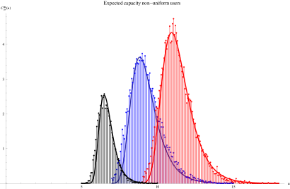
Figure 9: Bars are simulation results, while the solid lines represent analytic results. The middle, blue lob, represents the expected capacity for $K=1000$ users in non-uniform environment, where the channel capacity of each user follows Gaussian distribution with $\sigma_{i}\sim U[0.03,3]$ and $\mu_{i}\sim U[\sqrt{2}-1,\sqrt{2}+1]$, by the analysis in Theorem 3. Right side graph represents the expected capacity when all users have the same channel capacity as the capacity of the strongest user. Left side graph represents the capacity when all users have the same channel capacity as the capacity of the mean user.

In Figure 9 we present analytical results and simulated results of the expected capacity in a non-uniform environment for $K=1000$ users, and compare it to the expected capacity in a uniform environment.

4.1 Weighted Users

In this section, we derive the expected capacity when applying QoS to the users. The QoS refers to communication systems that allow the transport of traffic with special requirements, e.g., media streaming, IP telephony, online games and more. In particular, a certain minimum level of bandwidth and a certain maximum latency is required to function. In our setting, the QoS is reflected in the exceedance probability applied to each user. This reflection allows simple analysis, which is similar to heterogeneous users analysis. Hence, given a probability vector $\vec{p}\in\mathbb{R}^{K\times 1}$, each user sets a threshold corresponding to his exceedance probability by using (3.1) or by using (17), such that his threshold arrival rate corresponds to the QoS applied to him. Let $C_{av}^{QoS}\left(\vec{p}\right)$ denote the expected capacity in a non-uniform environment, when QoS applied to the users.

Claim 6.

The expected capacity with QoS in a non-uniform environment is

$$C_{av}^{QoS}\left(\vec{p}\right)=\frac{1}{K}\Lambda_{T}^{(\vec{p})}e^{-\frac{1}{K}\Lambda_{T}^{(\vec{p})}}\sum_{i=1}^{K}\frac{\Lambda_{i}^{(p_{i})}}{\Lambda_{T}^{(\vec{p})}}\left(\sigma_{i}\left[b_{1/p_{i}}-a_{1/p_{i}}\log\log\left(1-p_{i}\right)+a_{K}\right]+\mu_{i}+o(a_{1/p_{i}})\right)$$ (31)

where

$$\Lambda_{i}^{(p_{i})} = \exp\left\{-\frac{b_{K}+b_{1/p_{i}}}{a_{K}}\right\}\left(-\log(1-p_{i})\right)^{a_{1/p_{i}}},$$ (32)

$$\Lambda_{T}^{(\vec{p})} = \sum_{i=1}^{K}\Lambda_{i}^{(p_{i})}$$ (33)

and $p_{i}$ is the exceedance probability of the $i_{th}$ user.

Note that Claim 6 can be applied whether the users are uniformly distributed or not. That is, the QoS setting is applicable both in the previous, uniform case and in the later non-homogeneous case.

Proof.

Since

$$C_{av}^{QoS}=\Pr\left(\textmd{utilized slot}\right)E\left\{C|C_{i}>u_{i}\forall_{i=1,2,...,K}\right\}$$

We analyze the following. In (24), we expressed the threshold arrival rate as a function of the threshold $u$. Now, based on (17), we wish to set a unique threshold $u_{p_{i}}$ for each user, such that the $i_{th}$ user will exceed his threshold with probability $p_{i}$. Hence,

$$\Lambda_{i}^{(p_{i})} = \exp\left\{-\frac{u_{p_{i}}-\sigma_{i}b_{K}-\mu_{i}}{\sigma_{i}a_{K}}\right\}$$

$$= \exp\left\{\frac{-(b_{1/p_{i}}+b_{K})+a_{1/p_{i}}\left(\log\log(1-p_{i})\right)}{a_{K}}\right\}$$

$$= \exp\left\{-\frac{b_{K}+b_{1/p_{i}}}{a_{K}}\right\}\left(-\log(1-p_{i})\right)^{a_{1/p_{i}}}.$$

Since the users are independent, the total threshold arrival rate is the sum of rates for all users. Thus,

$$\Lambda_{T}^{(\vec{p})}=\sum_{i=1}^{K}\exp\left\{-\frac{(b_{K}+b{1/p_{i}})}{a_{K}}\right\}\left(-\log(1-p_{i})^{a_{1/p_{i}}}\right).$$

As for the expected capacity, similarly to the previous section, each user that exceeds the threshold contributes a different capacity, corresponding to his threshold. Hence, by averaging the capacity that each user donates, we obtain,

$$E\left\{C|C_{i}>u_{i}\forall_{i=1,2,...,K}\right\} = \sum_{i=1}^{K}\frac{\Lambda_{i}^{(p_{i})}}{\Lambda_{T}^{(\vec{p})}}\left(u_{p_{i}}+\sigma_{i}a_{K}+o(a_{K})\right)$$

$$= \sum_{i=1}^{K}\frac{\Lambda_{i}^{(p_{i})}}{\Lambda_{T}^{(\vec{p})}}\left(\sigma_{i}\left[b_{1/p_{i}}-a_{1/p_{i}}\log\log\left(1-p_{i}\right)+a_{K}\right]+\mu_{i}+o(a_{1/p_{i}})\right)$$

Finally, the probability that a slot is utilized, i.e., a single user exceeds the threshold in interval length of $1/K$, is

$$\Pr\left(\textmd{utilized slot}\right)=\frac{1}{K}\Lambda_{T}^{(\vec{p})}e^{-\frac{1}{K}\Lambda_{T}^{(\vec{p})}}.$$

Hence, Claim 6 follows. ∎

4.2 Equal Time Sharing of Non-Uniform Users

Equal-time-sharing is a scheduling strategy for which the system resources are equally distributed among users or groups. Whereas implementing equal-time-sharing in a homogeneous environment is to apply a uniform random or round-robin scheduling strategy to users, implementing equal-time-sharing in a non-uniform environment is to set for each user a threshold that is relative to his own sample maxima probability, i,e. set $p_{i}=\frac{1}{K},\forall i=1,2,...,K$.

Let $C_{av}^{es}$ denote the expected capacity in a non-uniform environment, when there is an equal exceedance probability to all users.

Corollary 2.

The expected capacity with equal time sharing follows

$$C_{av}^{es}=\frac{1}{K}\Lambda_{T}^{(1)}e^{-\frac{1}{K}\Lambda_{T}^{(1)}}\sum_{i=1}^{K}\frac{1}{K}\left(\sigma_{i}\left[b_{K}+a_{K}\left(1-\log\log\left(\frac{K-1}{K}\right)\right)\right]+\mu_{i}\right)+o(a_{K}).$$

where

$$\Lambda_{T}^{(1)}=e^{-2\frac{b_{K}}{a_{K}}}K\left(-\log\left(\frac{K-1}{K}\right)\right)^{a_{K}}$$ (34)

Equal time sharing is a special case of QoS. By setting $p_{i}=1/K$ in (32) to all users, Corollary 2 follows.

5 Capture effect

Similar to the human auditory system, where the strongest speaker is filtered out of a crowed, the capture effect is a phenomenon associated with signal reception in which in case of a collision, the stronger of two signals will be received correctly at the receiver. In this paper, the capture effect directly implies less harmful collisions, hence a higher capacity. That is, this phenomenon overcomes the situation where collisions corrupt the packets involved, and it has been shown that capture effect increase throughput and decrease delay in variety of wireless networks including radio broadcasting, such as Aloha networks, 802.11 networks, Bluetooth radios and cellular systems [35, 36]. In our settings, the capture effect enables us to set a lower threshold, such that two users will exceed the threshold on average, which significantly reduced the probability of idle slot.

Whereas using EVT to examine the capture effect capacity gain is rather complicated, the point process technique enables us to obtain it easily. In this section we characterize the capture effect capacity gain, when the receiver can successfully receive the transmission of the stronger user if no collision, or a collision of two users at most occurs.

Proposition 2.

The expected capacity of non-uniform users subject to capture effect follows

$$C_{av}^{nuc}(u) = \frac{1}{K}\Lambda_{T}e^{-\frac{1}{K}\Lambda_{T}}\left(\sum_{i=1}^{K}\frac{\Lambda_{i}}{\Lambda_{T}}(u+\sigma_{i}a_{K})\right)$$

$$+\frac{1}{2}\left(\frac{1}{K}\Lambda_{T}\right)^{2}e^{-\frac{1}{K}\Lambda_{T}}\left(\sum_{i=1}^{K}\sum_{j=i+1}^{K}2\frac{\Lambda_{i}\Lambda_{j}}{\Lambda_{T}^{2}}\left(u+\left(\sigma_{i}+\sigma_{j}-\frac{\sigma_{i}\sigma_{j}}{\sigma_{i}+\sigma_{j}}\right)a_{K}\right)\right)$$

$$+o(a_{K}).$$

where $\Lambda_{i}$ and $\Lambda_{T}$ are given in (24) and (25), respectively, and $a_{K}$ and $b_{K}$ are given in (5) and (6), respectively.

Proof.

The expected capacity obtained when a single user exceeds the threshold was given in Theorem 3. To obtain the expected capacity when two users exceed threshold in a $1/K$ slot interval we define the following events:

$$A_{t} = \textmd{exactly two users exceeded}.$$

$$A_{i} = \textmd{user i exceeded}.$$

$$A_{j} = \textmd{user j exceeded}.$$

The probability that only users $i$ and $j$ exceed threshold in a $1/K$ time interval follows

$$\Pr(A_{i},A_{j},A_{t}) = \frac{1}{K}\Lambda_{i}e^{-\frac{1}{K}\Lambda_{i}}\frac{1}{K}\Lambda_{j}e^{-\frac{1}{K}\Lambda_{j}}\prod_{l\neq j,i}e^{-\frac{1}{K}\Lambda_{l}}$$

$$= \frac{1}{K^{2}}\Lambda_{i}\Lambda_{j}e^{-\frac{1}{K}\Lambda_{T}}$$

$$= \frac{\left(\frac{1}{K}\Lambda_{T}\right)^{2}}{2}e^{-\frac{1}{K}\Lambda_{T}}2\frac{\Lambda_{i}\Lambda_{j}}{\Lambda_{T}^{2}}$$

When two users' capacities are above the threshold, the receiver captures only the stronger user transmission, hence, only the stronger user capacity counts in practice. The stronger user capacity distribution equals to the distribution of the maximum between two random capacities, which both have exponential tail distribution, that is, the maximum of two exponential random variables.

$$F_{\max\left(C_{i},C_{j}\right)|C_{i},C_{j}>u}(x) = \left(1-e^{-\frac{x}{\sigma_{i}a_{K}}}\right)\left(1-e^{-\frac{x}{\sigma_{j}a_{K}}}\right)$$

$$= 1-(e^{-\frac{x}{\sigma_{i}a_{K}}}+e^{-\frac{x}{\sigma_{j}a_{K}}})+e^{-\frac{x}{a_{K}}\frac{\sigma_{i}\sigma_{j}}{\sigma_{i}+\sigma_{j}}}.$$

Thus, when users $i$ and $j$ exceed the threshold, the stronger user will contribute

$$u+\left(\sigma_{i}+\sigma_{j}-\frac{\sigma_{i}\sigma_{j}}{\sigma_{i}+\sigma_{j}}\right)a_{K}.$$

to the expected capacity. Hence, by averaging the stronger user contribution among all $i$ and $j$, Proposition 2 follows. ∎

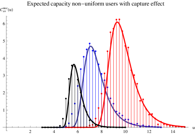
Figure 10: Expected capacity with capture effect for 250 users. On the left we present the capacity of uniform users, as if they see the same channel of the mean user, subject to capture effect. In the middle, we present the capacity of non-uniform users, subject to capture effect. On the left, we present the capacity of uniform users, as if they see the same channel of the mean user, subject to capture effect.

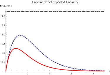
Figure 11: Capture effect capacity gain for 1000 i.i.d. users. The solid line represent the expected capacity when setting a threshold such that $k$ user exceeds the threshold on average, as given in Figure 5. The dashed line represent the expected capacity when $k$ users, that are subject to the capture effect, exceed the threshold on average. The upper dot-dashed line represent the expected capacity of the optimal multi-user diversity centralized scheme.

In Figure 10 we present the expected capacity for a uniform and non-uniform users, subject to the capture effect. In Figure 11 we present the capacity gain introduced by the capture effect, when setting a threshold such that $k$ user exceeds the threshold on average, and compare it to the expected capacity with no capture effect. Furthermore, we see that a higher capacity is achieved when setting a lower threshold, such that $k>1$ users will exceed it on average.

One should notice that the capture effect violates any QoS applied to users. When users subject to a QoS, each user must exceed a unique threshold corresponding to his QoS. Hence, when a collision occur, a strong user with a higher threshold, usually corresponding to a lower QoS, will utilize the threshold, violating the QoS guaranteed to users with lower threshold that usually corresponds to higher QoS.

6 Collision Avoidance

In this section, we show an algorithm which asymptotically achieves the optimal capacity. In [20, 24], the authors give a splitting algorithm that can cope with collisions when a collision detection mechanism is available, by dividing each slot into mini-slots, such that a collision can be resolved in the next mini-slot. In many cases, while collision resolution is not possible, the users are still capable of sensing the carrier, and understanding if a mini-slot is being used or not. Thus, we wish to develop a collision avoidance algorithm which is based only on carrier sensing. In other words, in this case we assume that the users are only able to detect if the channel is being used in mini-slots resolution. If a collision does occur within a mini-slot, we assume the whole slot is lost. First, we wish to minimize the idle slot probability, that without any enhancement will occur $1/e$ of the time. Next, we suggest an algorithm that copes with the resulting collision probability.

From (3.4), it is easy to see that the idle slot probability goes to zero when setting $k=\log K$ as follows,

$$\Pr(\textmd{ idle time slot })\rightarrow e^{-\log K}=1/K\rightarrow 0.$$

However, when setting a threshold such that $\log K$ users will exceed on average, we have to deal with $\log K$ users on average, that find themselves adequate for utilizing next time slot.
To overcome this problem, we suggest to rate users that exceeded the threshold by the distance they reached from the threshold. The set of values above the threshold is divided to $l$ bins: $[u_{p},u_{p}+t_{1}),[u_{p}+t_{1},u_{p}+t_{2}),\ldots,[u_{p}+t_{l-1},\infty)$, numbered $1,\ldots,l$, respectively. A user which passed the threshold checks in which bin its expected capacity lies. If the bin index is $i$, it waits $i$ mini-slots and checks the channel. If the channel is clean, it transmits its data. In order to achieve uniform distribution over the bins, we set the bins boundaries by the exponential limit distribution that we found in (20), that is, the $i_{th}$ bin boundaries follows

$$t_{i}=(2\log K)^{-1/2}\log(i/l),\qquad\forall i=1,2,...,l.$$

as we can see in Figure 12.

From now on, we assume that the probability for a user who passed the threshold to fall in a specific bin is $\frac{1}{l}$ for all bins.

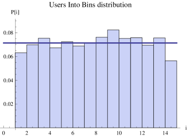
Figure 12: Distribution of users inside our bin when bin boundaries was set by (6)

Claim 7.

In the suggested enhanced scheme, the probability of utilized slot is

$$\Pr(\textmd{utilized slot})=\sum_{j=1}^{l}\sum_{m=1}^{K}\binom{K}{m}\left(\frac{k}{K}\right)^{m}\left(\frac{K-k}{K}\right)^{K-m}m\left(\frac{1}{l}\right)\left(\frac{l-j}{l}\right)^{m-1}$$

where $m$ is a realization of the number of uses who passed the threshold.

Proof.

Let $J$ be the index of the occupied bin with the lowest index, in which the strongest user lies. Thus, the probability that a single user occupies bin $J$, for a fixed $k$ users who exceeded the threshold is

$$\Pr\left(\textmd{ utilized slot }\right) = \sum_{j=1}^{l}k\left(\frac{1}{l}\right)\left(\frac{l-j}{l}\right)^{k-1}$$

We notice that when $k$ is not fixed, it should be represented as a random variable which follows the binomial distribution with parameters $n=K$ and $p=k/K$, as follows from (3.4). Hence, by using complete probability formula, we have

$$\Pr(\textmd{utilized slot}) = \Pr(E_{1})$$

$$= \sum_{j=1}^{l}\sum_{m=1}^{K}\binom{K}{m}\left(\frac{k}{K}\right)^{m}\left(\frac{K-k}{K}\right)^{K-m}m\left(\frac{1}{l}\right)\left(\frac{l-j}{l}\right)^{m-1}.$$

∎

This suggests that we can achieve small collision probability as we like, by increasing the number of bins, as the following claim asserts.

Claim 8.

In the enhanced algorithm the probability of unutilized slot converges to zero as $l$ increases.

Proof.

If there are $k$ users above threshold and $l$ bins then the probability that all $k$ fall into different bins is

$$\left(1-\frac{1}{l}\right)\cdot\left(1-\frac{2}{l}\right)\cdot...\cdot\left(1-\frac{k-1}{l}\right)=\prod_{j=1}^{k-1}\left(1-\frac{j}{l}\right)$$

Using that $1-k/l\leq e^{-k/l}$ is tight bound when $k$ is small compared to $l$, we have

$$\prod_{j=1}^{k-1}\left(1-\frac{j}{l}\right) \leq \prod_{j=1}^{k-1}e^{-j/l}$$

$$= \exp\left\{-\sum_{j=1}^{k-1}\frac{j}{l}\right\}$$

$$= e^{-k(k-1)/2l}$$

Hence, the probability of collision in any bin is $1-e^{-k(k-1)/2l}$, which is going to zero as $l$ increases. Hence, Claim 8 follows. ∎

6.1 Analyzing the Delay

Regardless of collisions that may occur, we analyze the expected time that took the maximal user decide that he is the most adequate to utilize a slot, which is equivalent to the expected index of the maximal occupied bin, out of $l$ bins. In order to obtain this, we order the bins in descending order, such that bin $1$ corresponds to the highest capacities. Since we choose $k\ll K$, on average only a small group of users will exceed the threshold, thus, we can express the probability that bin $j$ is maximal, without using extreme distributions.
Let $J$ denote the index of the maximal user bin, we obtain the following.

Claim 9.

For a random number of users that exceeded threshold $u_{p}$, the expected maximal bin index $J$ follows

$$E[J]=\sum_{j=1}^{l}\sum_{m=1}^{K}\binom{K}{m}\left(\frac{k}{K}\right)^{m}\left(\frac{K-k}{K}\right)^{K-m}\left(\frac{l-j}{l}\right)^{m}.$$

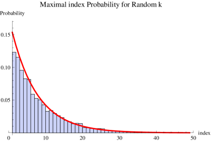
Figure 13: maximal index simulation and analysis for random k, where the line follows (Remark).

Proof.

Given $k$ users that exceeded threshold we obtain

$$E[J|k\textmd{ users exceeded}] = \sum_{j=1}^{l}\Pr(\left.J>j\right|k\textmd{ user exceeded})$$

$$= \sum_{j=1}^{l}\left(\frac{l-j}{l}\right)^{k}.$$

By the law of total expectation we obtain the expected maximal bin index $J$, for random k of users as follows.

$$E[J] = E_{\textbf{k}}\left[E[J|\textbf{k}\textmd{ users exceeded}]\right]$$

$$= \sum_{j=1}^{l}\sum_{m=1}^{K}\Pr(\textbf{k}=m)\Pr(\left.J>j\right|\textbf{k}=m)$$

$$= \sum_{j=1}^{l}\sum_{m=1}^{K}\binom{K}{m}\left(\frac{k}{K}\right)^{m}\left(\frac{K-k}{K}\right)^{K-m}\left(\frac{l-j}{l}\right)^{m}.$$

Hence, Claim 9 follows. ∎

Remark.

The probability that bin $J=j$ is maximal for a fixed $k$ users who exceeded the threshold follows

$$\Pr(J=j) = \sum_{m=1}^{K}\Pr(\textbf{k}=m)\Pr\left(J=j|\textbf{k}=m\right)$$

$$= \sum_{m=0}^{K}\binom{K}{m}\left(\frac{k}{K}\right)^{m}\left(1-\frac{k}{K}\right)^{K-m}\left(\left(\frac{l-j+1}{l}\right)^{m}-\left(\frac{l-j}{l}\right)^{m}\right).$$

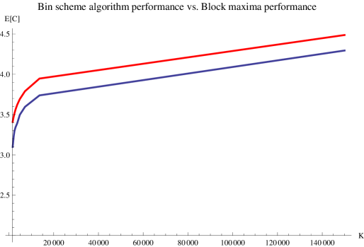
Figure 14: Bottom line - Threshold scheme expected capacity for K users, setting threshold that on average $\lceil\log K\rceil$ users exceeds threshold, placing them into $(\lceil\log K\rceil)^{2}$ bins with the boundaries obtained in (6).Top line is the optimal centralized scheme performance.

In Figure 14 we see the enhanced algorithm performance when setting a threshold such that $\lceil\log K\rceil$ users exceed it on average, then placing them into $(\lceil\log K\rceil)^{2}$ mini-slots, comparing to the optimal centralized scheduler.

7 Conclusion

In this paper, we presented a distributed scheduling scheme for exploiting multiuser diversity in a non-uniform environment, where each user has a different location, therefor will experience different channel distribution. We characterized the scaling law of the expected capacity and the system throughput by a point process approximation, and presented a simple analysis for the expected value and throughput when applying QoS upon users. Moreover, we presented an enhancement for the distributed algorithm in which the expected capacity and throughput reaches the optimal capacity, for a small delay price.

Appendix A Appendix A

In this section we derive the constants $a_{n}$ and $b_{n}$, for the Gaussian case.

Proof.

We denote the standard normal distribution function and density function by $\Phi$ and $\phi$ respectively, and notice the relation of the tail of $\Phi$, for positive values of $x$, from Taylor series:

$$1-\Phi(x)\leq\frac{\phi(x)}{x}$$ (40)

with equality when $x\rightarrow\infty$.

First, we wish to find where $\xi$ converges to. I.e., to what distribution type the maxima of Gaussian distribution converges. Thus, we use the relation in (40) to derive the shape parameter of Gaussian maxima,

$$\xi \approx \frac{d}{dx}\left[\frac{\phi(x)/x}{\phi(x)}\right]$$

$$\approx \frac{d}{dx}\frac{1}{x}\rightarrow 0$$

we substitute $\xi\rightarrow 0$ in (2), and find the limit distribution from extreme value theory

$$\Pr(M_{n}\leq u) = \left[\Phi(u)\right]^{n}$$

$$= \exp\left[-(1+\xi\frac{u-b_{n}}{a_{n}})\right]^{-\frac{1}{\xi}}$$

$$\stackrel{{\scriptstyle\xi\rightarrow 0}}{{\longrightarrow}} \exp[-e^{-\left(\frac{u-b_{n}}{a_{n}}\right)}].$$

That is, the maxima of Gaussian random variables converges to Gumbel distribution, where $u=a_{n}x+b_{n}$.

For retrieving the normalizing constants, $a_{n}$ and $b_{n}$, as can be found rigorously at [29, Theorem 1.5.3.], we use a well known $\log$ approximation for large values of $x$,

$$-\log[1-(1-x)]\geq 1-x$$

and apply it to (A), i.e.,

$$-\log[\Phi(u)]^{n}=-n\log(1-[1-\Phi(u)])\geq n\left(1-\Phi(u)\right)\\$$ (42)

hence,

$$n\left(1-\Phi(u)\right)\longrightarrow(1+\xi x)^{-\frac{1}{\xi}}$$ (43)

apply $\xi\rightarrow 0$ to (43), thus,

$$n\left(1-\Phi(u)\right)\stackrel{{\scriptstyle\xi\rightarrow 0}}{{\longrightarrow}}e^{-x}.$$ (44)

So, in oreder to satisfy (44), we shell take $1-\Phi(u)=\frac{1}{n}e^{-x}$.
Using again the tail relation (40), we obtain,

$$\frac{1}{n}e^{-x}\sim\frac{\phi(u)}{u}$$

or

$$\frac{1}{n}e^{-x}\frac{u}{\phi(u)}\stackrel{{\scriptstyle x\rightarrow\infty}}{{\longrightarrow}}1$$ (45)

applying $\log$ function on (45) will lead us to

$$-\log n-x+\log u-\log\phi(u)\longrightarrow 0$$ (46)

we substitute $\phi(u)$ for a Normal density function, $\frac{1}{\sqrt{2\pi}}e^{-\frac{1}{2}u^{2}}$ in (46),
hence,

$$-\log n-x+\log u+\frac{1}{2}\log 2\pi+\frac{u^{2}}{2}\longrightarrow 0$$ (47)

and by substitute $x=\frac{u-b_{n}}{a_{n}}$ in (47) and rearrange it a little, we obtain,

$$-\left(\frac{u-b_{n}}{a_{n}}\right)+\log u+\frac{1}{2}\log 2\pi+\frac{u^{2}}{2}\longrightarrow\log n$$

and since $u^{2}$ has the main influence on the left hand side, it implies that

$$\frac{u^{2}}{2\log n}\longrightarrow 1$$ (48)

hence, by applying $\log$ to (48), we obtain

$$2\log u-\log 2-\log\log n\longrightarrow 0$$

or

$$\log u=\frac{1}{2}\left(\log 2+\log\log n\right)+o(1).$$ (49)

We place (49) in (47),and rearrange it a little to obtain

$$u^{2} = 2\log n\left[(\log n)^{-1}x+1\right.+$$

$$-\frac{1}{2}(\log n)^{-1}\left(\log 4\pi+\log\log n\right)+\left.o(\frac{1}{\log n})\right]$$

and hance,

$$u = 2(\log n)^{\frac{1}{2}}\left[\frac{x}{(2\log n)}+1+\right.$$

$$-\left.\frac{\frac{1}{2}\left(\log 4\pi+\log\log n\right)}{(2\log n)}+o(\frac{1}{\log n})\right]$$

$$= (2\log n)^{-\frac{1}{2}}x+(2\log n)^{\frac{1}{2}}+$$

$$-\frac{1}{2}(2\log)^{-\frac{1}{2}}\left(\log\log n+\log 4\pi\right)+o\left(\frac{1}{(\log n)^{\frac{1}{2}}}\right)$$

$$= a_{n}x+b_{n}+o(a_{n})$$

which means that (A) follows for

$$a_{n}=(2\log n)^{-\frac{1}{2}}$$

and

$$b_{n}=(2\log n)^{\frac{1}{2}}-\frac{1}{2}(2\log n)^{-\frac{1}{2}}[\log\log n+\log(4\pi)].$$

∎

Appendix B Appendix C

Proof.

(Theorem 2) Let $N_{n}(B)$ and $N(B)$ be the number of points of $P_{n}$ and $P$ respectively in set $B$.
Assuming that for any $n$ disjoint sets $B_{1},B_{2},...,B_{n}$, with $B_{i}\subset C,\forall i=1,2..,n$, then $N(B_{1}),N(B_{2}),...,N(B_{n})$ are independent random variables. we will show that as $n\rightarrow\infty$

$$E(N_{n}(B))\longrightarrow E(N(B))$$

and

$$\Pr(N_{n}(B)=0)\longrightarrow\Pr(N(B)=0).$$

Thus, we take $B_{v}=(0,1]\times(v,\infty)$, such that the $i_{th}$ point of $P_{n}$ is in $B_{v}$ if

$$\frac{\textbf{x}_{i}-b_{n}}{a_{n}}>v$$

i.e., if $\textbf{x}_{i}>a_{n}v+b_{n}$.
The probability of this is $1-F(a_{n}v+b_{n})$.
Hence, the expected number of such points is

$$E[N_{n}(B_{v})] = n[1-F(a_{n}v+b_{n})]$$

$$\leq -\log\left[F(a_{n}v+b_{n})\right]^{n}$$

$$\rightarrow -\log G(v)$$

$$= (1+\xi v)_{+}^{-\frac{1}{\xi}}$$

$$= \Lambda(B_{v})$$

$$= E[N(B_{v})].$$

Similarly, the event $N_{n}(B_{v})=0$ can be expressed as

$$\{N_{n}(B_{v})\} = \left\{\frac{\textbf{x}_{i}-b_{n}}{a_{n}}\leq v,\forall i=1,...,n\right\}$$

$$= \left\{\textbf{x}_{i}\leq a_{n}v+b_{n}\forall i=1,...,n\right\}$$

So

$$\Pr(N_{n}(B_{v})=0) = \{F(a_{n}v+b_{n})\}^{n}$$

$$\rightarrow G(v)$$

$$= \exp[-(1+\xi v)_{+}^{-1/\xi}]$$

$$= \exp[-\Lambda(B_{v})]$$

$$= \Pr(N(B_{v})=0)$$

∎

References

- [1] H. Weingarten, Y. Steinberg, and S. Shamai, ``The capacity region of the gaussian multiple-input multiple-output broadcast channel,'' Information Theory, IEEE Transactions on, vol. 52, no. 9, pp. 3936–3964, 2006.
- [2] S. Sesia, I. Toufik, and M. Baker, ``Lte–the umts long term evolution,'' From Theory to Practice, published in, vol. 66, 2009.
- [3] I. S. for Local and metropolitan area networks, Part 16: Air Interface for Broadband Wireless Access Systems Amendment 3: Advanced Air Interface. pub-IEEE-STD, May 2011.
- [4] R. Knopp and P. Humblet, ``Information capacity and power control in single-cell multiuser communications,'' in IEEE International Conference on Communications, Seattle, vol. 1, 1995, pp. 331–335.
- [5] T. Yoo and A. Goldsmith, ``On the optimality of multiantenna broadcast scheduling using zero-forcing beamforming,'' Selected Areas in Communications, IEEE Journal on, vol. 24, no. 3, pp. 528–541, 2006.
- [6] R. Zakhour and S. Hanly, ``Min-max fair coordinated beamforming via large system analysis,'' IEEE International Symposium on Information Theory Proceedings, pp. 1896–1900, 2011.
- [7] C. Chen and L. Wang, ``Enhancing coverage and capacity for multiuser mimo systems by utilizing scheduling,'' Wireless Communications, IEEE Transactions on, vol. 5, no. 5, pp. 1148–1157, 2006.
- [8] K. Jagannathan, S. Borst, P. Whiting, and E. Modiano, ``Scheduling of multi-antenna broadcast systems with heterogeneous users,'' Selected Areas in Communications, IEEE Journal on, vol. 25, no. 7, pp. 1424–1434, 2007.
- [9] M. Sharif and B. Hassibi, ``A comparison of time-sharing, dpc, and beamforming for mimo broadcast channels with many users,'' Communications, IEEE Transactions on, vol. 55, no. 1, pp. 11–15, 2007.
- [10] G. Caire, ``Mimo downlink joint processing and scheduling: a survey of classical and recent results,'' in Proc. Workshop on Information Theory and Its Applications, 2006.
- [11] B. Hassibi and M. Sharif, ``Fundamental limits in mimo broadcast channels,'' Selected Areas in Communications, IEEE Journal on, vol. 25, no. 7, pp. 1333–1344, 2007.
- [12] W. Choi and J. Andrews, ``The capacity gain from intercell scheduling in multi-antenna systems,'' Wireless Communications, IEEE Transactions on, vol. 7, no. 2, pp. 714–725, 2008.
- [13] L. Wang, C. Chiu, C. Yeh, and C. Li, ``Coverage enhancement for ofdm-based spatial multiplexing systems by scheduling,'' in IEEE Wireless Communications and Networking Conference, WCNC. IEEE, 2007, pp. 1439–1443.
- [14] M. Pun, V. Koivunen, and H. Poor, ``Opportunistic scheduling and beamforming for mimo-sdma downlink systems with linear combining,'' in IEEE 18th International Symposium on Personal, Indoor and Mobile Radio Communications, 2007, pp. 1–6.
- [15] J. Choi and F. Adachi, ``User selection criteria for multiuser systems with optimal and suboptimal lr based detectors,'' Signal Processing, IEEE Transactions on, vol. 58, no. 10, pp. 5463–5468, 2010.
- [16] M. Airy, S. Shakkattai, and R. Heath Jr, ``Spatially greedy scheduling in multi-user mimo wireless systems,'' in the Thirty-Seventh Asilomar Conference on Signals, Systems and Computers, vol. 1. IEEE, 2003, pp. 982–986.
- [17] C. Swannack, E. Uysal-Biyikoglu, and G. Wornell, ``Low complexity multiuser scheduling for maximizing throughput in the mimo broadcast channel,'' in Proc. Allerton Conf. Communications, Control and Computing, 2004.
- [18] G. Primolevo, O. Simeone, and U. Spagnolini, ``Channel aware scheduling for broadcast mimo systems with orthogonal linear precoding and fairness constraints,'' in IEEE International Conference on Communications, vol. 4, 2005, pp. 2749–2753.
- [19] T. Yoo, N. Jindal, and A. Goldsmith, ``Finite-rate feedback mimo broadcast channels with a large number of users,'' in Information Theory, 2006 IEEE International Symposium on. IEEE, 2006, pp. 1214–1218.
- [20] X. Qin and R. Berry, ``Exploiting multiuser diversity for medium access control in wireless networks,'' in INFOCOM 2003. Twenty-Second Annual Joint Conference of the IEEE Computer and Communications. IEEE Societies, vol. 2. IEEE, 2003, pp. 1084–1094.
- [21] ——, ``Distributed approaches for exploiting multiuser diversity in wireless networks,'' Information Theory, IEEE Transactions on, vol. 52, no. 2, pp. 392–413, 2006.
- [22] K. Bai and J. Zhang, ``Opportunistic multichannel aloha: distributed multiaccess control scheme for ofdma wireless networks,'' Vehicular Technology, IEEE Transactions on, vol. 55, no. 3, pp. 848–855, 2006.
- [23] X. Qin and R. Berry, ``Distributed power allocation and scheduling for parallel channel wireless networks,'' Wireless Networks, vol. 14, no. 5, pp. 601–613, 2008.
- [24] ——, ``Opportunistic splitting algorithms for wireless networks,'' in INFOCOM 2004. Twenty-third AnnualJoint Conference of the IEEE Computer and Communications Societies, vol. 3. IEEE, 2004, pp. 1662–1672.
- [25] T. To and J. Choi, ``On exploiting idle channels in opportunistic multichannel aloha,'' Communications Letters, IEEE, vol. 14, no. 1, pp. 51–53, 2010.
- [26] P. Smith and M. Shafi, ``On a gaussian approximation to the capacity of wireless mimo systems,'' in Communications, 2002. ICC 2002. IEEE International Conference on, vol. 1. IEEE, 2002, pp. 406–410.
- [27] V. Girko, ``A refinement of the central limit theorem for random determinants,'' THEORY OF PROBABILITY AND ITS APPLICATIONS C/C OF TEORIIA VEROIATNOSTEI I EE PRIMENENIE, vol. 42, pp. 121–129, 1997.
- [28] M. Chiani, M. Win, and A. Zanella, ``On the capacity of spatially correlated mimo rayleigh-fading channels,'' Information Theory, IEEE Transactions on, vol. 49, no. 10, pp. 2363–2371, 2003.
- [29] M. Leadbetter, Extremes and Related Properties of Random Sequences and Processes. Springer-Verlag, N.Y, 1983.
- [30] S. Coles, An introduction to statistical modeling of extreme values. Springer Verlag, 2001.
- [31] E. Eastoe and J. Twan, ``M453 extremes emma eastoe and jonathan tawn,'' 2007.
- [32] L. De Haan and A. Ferreira, Extreme value theory: an introduction. Springer Verlag, 2006.
- [33] R. Smith, ``Extreme value analysis of environmental time series: an application to trend detection in ground-level ozone,'' Statistical Science, vol. 4, no. 4, pp. 367–377, 1989.
- [34] J. Galambos, J. Lechner, and E. Simiu, Extreme value theory and applications: proceedings of the Conference on Extreme Value Theory and Applications, Gaithersburg, Maryland, 1993. Springer, 1994, vol. 1.
- [35] K. Whitehouse, A. Woo, F. Jiang, J. Polastre, and D. Culler, ``Exploiting the capture effect for collision detection and recovery,'' in Embedded Networked Sensors, 2005. EmNetS-II. The Second IEEE Workshop on. IEEE, 2005, pp. 45–52.
- [36] Z. Hadzi-Velkov and B. Spasenovski, ``Capture effect in ieee 802.11 basic service area under influence of rayleigh fading and near/far effect,'' in Personal, Indoor and Mobile Radio Communications, 2002. The 13th IEEE International Symposium on, vol. 1. IEEE, 2002, pp. 172–176.