A SIMPLE DERIVATION OF NEWTON-COTES FORMULAS WITH REALISTIC ERRORS

Abstract

In order to approximate the integral $I(f)=\int_{a}^{b}f(x)dx$, where $f$ is a sufficiently smooth function, models for quadrature rules are developed using a given panel of $n\,\,(n\geq 2)$ equally spaced points. These models arise from the undetermined coefficients method, using a Newton’s basis for polynomials. Although part of the final product is algebraically equivalent to the well known closed Newton-Cotes rules, the algorithms obtained are not the classical ones.

In the basic model the most simple quadrature rule $Q_{n}$ is adopted (the so-called left rectangle rule) and a correction $\tilde{E}_{n}$ is constructed, so that the final rule $S_{n}=Q_{n}+\tilde{E}_{n}$ is interpolatory. The correction $\tilde{E}_{n}$, depending on the divided differences of the data, might be considered a realistic correction for $Q_{n}$, in the sense that $\tilde{E}_{n}$ should be close to the magnitude of the true error of $Q_{n}$, having also the correct sign. The analysis of the theoretical error of the rule $S_{n}$ as well as some classical properties for divided differences suggest the inclusion of one or two new points in the given panel. When $n$ is even it is included one point and two points otherwise. In both cases this approach enables the computation of a realistic error $\bar{E}_{S_{n}}$ for the extended or corrected rule $S_{n}$. The respective output $(Q_{n},\tilde{E}_{n},S_{n},\bar{E}_{S_{n}})$ contains reliable information on the quality of the approximations $Q_{n}$ and $S_{n}$, provided certain conditions involving ratios for the derivatives of the function $f$ are fulfilled. These simple rules are easily converted into composite ones. Numerical examples are presented showing that these quadrature rules are useful as a computational alternative to the classical Newton-Cotes formulas.

Keywords: Divided differences; undetermined coefficients method; realistic error; Newton-Cotes rules.

AMS Subject Classification: 65D30, 65D32, 65-05, 41A55.

1 Introduction

The first two quadrature rules taught in any numerical analysis course belong to a group known as closed Newton-Cotes rules. They are used to approximate the integral $I(f)=\int_{a}^{b}f(x)dx$ of a sufficiently smooth function $f$ in the finite interval $[a,b]$. The basic rules are known as trapezoidal rule and the Simpson’s rule. The trapezoidal rule is $Q(f)=h/2\,(f(a)+f(b))$, for which $h=b-a$, and has the theoretical error

$$\begin{array}[]{l}I(f)-Q(f)=-\displaystyle{\frac{h^{3}}{12}}\,f^{(2)}(\xi),\end{array}$$ (1)

while the Simpson’s rule is $Q(f)=h/3\,(f(a)+4\,f((a+b)/2)+f(b))$, with $h=(b-a)/2$, and its error is

$$\begin{array}[]{l}I(f)-Q(f)=-\displaystyle{\frac{h^{5}}{90}}\,f^{(4)}(\xi).\end{array}$$ (2)

The error formulas (1) and (2) are of existential type. In fact, assuming that $f^{(2)}$ and $f^{(4)}$ are (respectively) continuous, the expressions (1) and (2) say that there exist a point $\xi$, somewhere in the interval $(a,b)$, for which the respective error has the displayed form. From a computational point of view the utility of these error expressions is rather limited since in general is quite difficult or even impossible to obtain expressions for the derivatives $f^{(2)}$ or $f^{(4)}$, and consequently bounds for $|I(f)-Q(f)|_{\infty}$. Even in the case one obtains such bounds they generally overestimate the true error of $Q(f)$.

Under mild assumption on the smoothness of the integrand function $f$, our aim is to determine certain quadrature rules, say $R(f)$, as well as approximations for its error $\tilde{E}(f)$, using only the information contained in the table of values or panel arising from the discretization of the problem. The algorithm to be constructed will produce the numerical value $R(f)$, the correction or estimated error $\tilde{E}(f)$ as well as the value of the interpolatory rule

$$S(f)=R(f)+\tilde{E}(f).$$ (3)

The true error of $S(f)$ should be much less than the estimated error of $R(f)$, that is,

$$|I(f)-S(f)|<<|\tilde{E}(f)|,$$ (4)

for a sufficiently small step $h$. In such case we say that $\tilde{E}(f)$ is a realistic correction for $R(f)$. Unlike the usual approach where one builds a quadrature formula $Q(f)$ (like the trapezoidal or Simpson’s rule) which is supposed to be a reasonable approximation to the exact value of the integral, here we do not care wether the approximation $R(f)$ is eventually bad, provided that the correction $\tilde{E}(f)$ has been well modeled. In this case the value $S(f)$ will be a good approximation to the exact value of the integral $I(f)$. Besides the values $R(f)$, $\tilde{E}(f)$ and $S(f)$ we are also interested in computing a good estimation $\bar{E}_{S}(f)$ for the true error of $S(f)$, in the following sense. If the true error $E(f)=I(f)-S(f)$ is expressed in the standard decimal form as $E(f)=\pm 0.d_{1}d_{2}\cdots d_{m}\times 10^{-k},\,\,k\geq 0$, the approximation $\bar{E}(f)$ is said to be realistic if its decimal form has the same sign as $E(f)$ and its first digit in the mantissa differs at most one unit, that is, $\bar{E}(f)=\pm 0.(d_{1}\pm 1)\,\cdots\,\times 10^{-k}$ (the dots represent any decimal digit). Finally, the algorithm to be used will produce the values $(R(f),\tilde{E}(f),S(f),\bar{E}(f))$.

In section 1.1 we present two models for building simple quadrature rules named model $A$ and model $B$. Although both models are derived from the same method, in this work we focus our attention mainly on the model $A$. Definitions, notations and background material are presented in section 2. In Proposition 2.1 we obtain the weights for the quadrature rule in model $A$ by the undetermined coefficients method as well as the theoretical error expressions for the rules are deduced (see Proposition 2.4). The main results are discussed in Section 3, namely in Proposition 3.1 we show that a reliable computation of realistic errors depends on the behavior of a certain function involving ratios between high order derivatives of the integrand function $f$ and its first derivative.

Composite rules for model A are presented in Section 4 where some numerical examples illustrate how our approach allows to obtain realistic error’s estimates for these rules.

1.1 Two models

In this work we consider to be given a panel of $n\,(n\geq 2)$ points $\{(x_{1},f_{1}),(x_{2},f_{2}),$ $\ldots,(x_{n},f_{n})\}$, in the interval $[a,b]$, having the nodes $x_{i}$ equally spaced with step $h>0$, $f_{i}=f(x_{i})$, where $f$ a sufficiently smooth function in the interval. We consider the following two models:

Model A

Using only the first node of the panel we construct a quadrature rule $Q_{n}(f)$ adding a correction $\tilde{E}_{n}(f)$, so that the corrected or extended rule $S_{n}(f)=Q_{n}(f)+\tilde{E}_{n}(f)$ is interpolatory for the whole panel,

$$S_{n}(f) =Q_{n}(f)+\tilde{E}_{n}(f)$$

$$=a_{1}\,f(x_{1})+\left\{a_{2}\,f[x_{1},x_{2}]+\cdots+a_{n}\,f[x_{1},x_{2},\ldots,x_{n}]\right\},$$ (5)

where $f[x_{1},x_{2},\ldots,x_{n}]$ denotes the $(n-1)$-th divided difference and $a_{1}$, $a_{2}$, $\ldots$, $a_{n}$ are weights to be determined.

Note that $Q_{n}(f)$ is simply the so-called left rectangle rule, thus $\tilde{E}_{n}(f)=\sum_{j=2}^{n}$ $a_{j}\,f[x_{1},\ldots,x_{j}]$ can be seen as a correction to such a rule.

Model B

The rule $Q_{n}(f)$ uses the first $n-1$ points of the panel (therefore is not interpolatory in the whole panel), and it is added a correction term $\tilde{E}_{n}(f)$, so that the corrected or extended rule $S_{n}(f)$ is interpolatory,

$$S_{n}(f) =Q_{n}(f)+\tilde{E}_{n}(f)$$

$$=\left\{\,a_{1}\,f(x_{1})+a_{2}\,f(x_{2})+\cdots+a_{n-1}\,f(x_{n-1})\,\right\}+a_{n}\,f[x_{1},x_{2},\ldots,x_{n}].$$ (6)

Since the interpolating polynomial of the panel is unique, the value computed for $S_{n}(f)$ using either model is the same and equal to the value one finds if the simple closed Newton-Cotes rule for $n$ equally spaced points has been applied to the data. This means that the extended rules (5) and (6) are both algebraically equivalent to the referred simple Newton-Cotes rules. However, the algorithms associated to each of the models (5) and (6) are not the classical ones for the referred rules. In particular, we can show that that for $n$ odd, the rules $Q_{n}(f)$ in model B are open Newton-Cotes formulas [3]. Therefore, the extended rule $S_{n}$ in model B can be seen as a bridge between open and closed Newton-Cotes rules.

The method of undetermined coefficients applied to a Newton’s basis of polynomials is used in order to obtain $S_{n}(f)$. The associated system of equations is diagonal, The same method can also be applied applied to get any hybrid model obtained from the models A and B. For instance, an hybrid extended rule using $n=3$ points could be written as

$$S_{3}(f)=\left\{a_{1}\,f(x_{1})+a_{2}\,f(x_{2})+a_{3}\,f(x_{3})\right\}+a_{4}\,f[x_{1},x_{2}]+a_{5}\,f[x_{1},x_{2},x_{3}].$$

In this work our study is mainly focused in model $A$.

2 Notation and background

Definition 2.1.

(Canonical and Newton’s basis)

Let ${\cal P}_{k}$ be the vector space of real polynomials of degree less or equal to $k$ ($k$ a nonnegative integer). The set $\,<\phi_{0}(x),\phi_{1}(x),\-\ldots,\phi_{n-1}(x)>$, where

$$\phi_{i}(x)=x^{i},\quad i=0,1,\ldots,n-1,$$ (7)

is the canonical basis for ${\cal P}_{n-1}$.

Given $n\geq 1$ distinct points $x_{1},x_{2},\ldots x_{n}$, the set $<w_{0}(x),w_{1}(x),\ldots,w_{n-1}(x)>$, with

$$\begin{array}[]{l}w_{0}(x)=1\\ w_{i}(x)=w_{i-1}(x)\times(x-x_{i}),\quad i=1,\ldots,(n-1)\end{array}$$ (8)

is known as the Newton’s basis for ${\cal P}_{n-1}$.

A polynomial interpolatory quadrature rule $R_{n}(f)$ obtained from a given panel $\{(x_{1},f_{1}),\-(x_{2},f_{2}),\ldots,(x_{n},f_{n})\}$, where $x_{i}\neq x_{j}$ for $i\neq j$, has the form

$$R_{n}(f)=c_{1}\,f(x_{1})+c_{2}\,f(x_{2})+\cdots+c_{n}f(x_{n}),$$ (9)

where the coefficients (or weights) $c_{j}\,\,(1\leq j\leq n)$ can be computed assuming the quadrature rule is exact for any polynomial $q$ of degree less or equal to $n-1$, that is, $deg(R_{n}(f))=n-1$, according to the following definition

Definition 2.2.

(Degree of exactness) ([2], p. 157)

A quadrature rule $R_{n}(f)=\sum_{i=1}^{n}c_{i}\,f(x_{i})$ has (polynomial) degree of exactness $d$ if the rule is exact whenever $f$ is a polynomial of degree $\leq d$, that is

$$E_{n}(f)=I(f)-R_{n}(f)=0\quad\mbox{for all}\quad f\,\in{\cal P}_{d}.$$

The degree of the quadrature rule is denoted by $deg(R)$. When $deg(R)=n-1$ the rule is called interpolatory.

In particular for a $n$-point panel the interpolating polynomial $p$ satisfies

$$f(x)=p(x)+r(x),\qquad x\,\in[a,b],$$ (10)

where $p$ can be written in Newton’s form (see for instance [6], p. 23, or any standard text in numerical analysis)

$$p(x)=f_{1}+f[x_{1},x_{2}]\,(x-x_{1})+\cdots+f[x_{1},x_{2},\ldots,x_{n}]\,(x-x_{1})\,(x-x_{2})\cdots(x-x_{n-1})\\$$ (11)

and the remainder-term is

$$r(x)=f[x_{1},x_{2},\ldots,x_{n},x]\,(x-x_{1})\,(x-x_{2})\cdots(x-x_{n}),$$ (12)

where $f_{i}=f(x_{i})$ and $f[x_{1},x_{2},\ldots,x_{1+j}]$, for $j\geq 0$, denotes the $j$-th divided difference of the data $(x_{i},f_{i})$, with $i=1,\ldots,n$. Therefore from (10) we obtain

$$I(f)=\int_{a}^{b}p(x)dx+\int_{a}^{b}r(x)dx=R_{n}(f)+E_{R_{n}}(f),$$ (13)

where $E_{R_{n}}(f)$ denotes the true error of the rule $R_{n}(f)$. Thus,

$$\begin{array}[]{ll}R_{n}(f)&=\int_{x_{1}}^{x_{n}}w_{0}(x)dx\times f_{1}+\int_{x_{1}}^{x_{n}}w_{1}(x)dx\times f[x_{1},x_{2}]+\cdots+\\ &+\int_{x_{1}}^{x_{n}}w_{n-1}(x)dx\times f[x_{1},x_{2},\ldots,x_{n}]\end{array}$$ (14)

The expression (14) suggests that the application of the undetermined coefficient method using the Newton’s basis for polynomials should be rewarding since the successive divided differences are trivial for such a basis. In particular, the weights for the extended rule in model A are trivially computed.

Proposition 2.1.

The weights for the rule $S_{n}(f)$ in model A are

$$a_{i}=I(w_{i-1})=\int_{0}^{(n-1)\,h}\,w_{i-1}(t)dt\qquad i=1,2,\ldots,n$$ (15)

Proof.

The divided differences do not depend on a particular node but on the distance between nodes. Thus for any given $n$-point panel of constant step $h$, we can assume without loss of generality that $x_{1}=0,x_{2}=h,\ldots,x_{n}=(n-1)\,h$. Considering the Newton’s basis for polynomials $w_{0}(t)=1$, $w_{1}(t)=t$, $\ldots$, $w_{n-1}(t)=t\,(t-h)\cdots(t-(n-2)\,h)$, where $0\leq t\leq(n-1)\,h$, from (5) we have

$$S_{n}(w_{0})=a_{1},\quad S_{n}(w_{1})=a_{2},\ldots,S_{n}(w_{i})=a_{i+1}\quad\mbox{for}\quad i=0,\ldots,(n-1).$$

The undetermined coefficients method applied to the Newton’s basis $<w_{0}(t)$, $w_{1}(t)$, $\ldots,w_{n-1}(t)>$ leads to the $n$ conditions $a_{i}=I(w_{i-1})$ or, equivalently, to a diagonal system of linear equations whose matrix is the identity. The equalities in (15) can also be obtained directly from (14). ∎

Theoretical expressions for the error $E_{R_{n}}(f)$ in (13) can be obtained either via the mean value theorem for integrals or by considering the so-called Peano kernel ([1], p. 285, [2], p. 176). However, we will use the method of undetermined coefficients whenever theoretical expressions for the errors $E_{Q_{n}}$ and $E_{S_{n}}$ are needed.

For sufficiently smooth functions $f$, the fundamental relationship between divided differences on a given panel and the derivatives of $f$ is given by the following well known result,

Proposition 2.2.

([6], p. 24),([2] p. 101]), ([5], p. 41)

Given $n\,\,(n\geq 2)$ distinct nodes $\{x_{1},\ldots,x_{n}\}$ in $J=[a,b]$, and $f\in C^{n-1}(J)$, there exists $\xi\in\,(x_{1},x_{n})$ such that

$$\begin{array}[]{l}f[x_{1},x_{2},\ldots,x_{n}]=\displaystyle{\frac{f^{(n-1)}(\xi)}{(n-1)!}}.\end{array}$$ (16)

Applying (16) to the canonical or Newton’s basis, we get

$$\begin{array}[]{l}\phi_{j}[x_{1},x_{2},\ldots,x_{n}]=w_{j}[x_{1},x_{2},\ldots,x_{n}]=0,\qquad\mbox{for}\quad j=0,1,\ldots,(n-2)\\ \phi_{n-1}[x_{1},x_{2},\ldots,x_{n}]=w_{n-1}[x_{1},x_{2},\ldots,x_{n}]=1.\end{array}$$ (17)

By construction, the rules $S_{n}$ in models $A$ and $B$ are at least of degree $n-1$ of precision according to Definition 2.2.

In this work the undetermined coefficients method enables us to obtain both the weights and theoretical error formulas. This apparently contradicts the following assertion due to Walter Gautschi ([2], p. 176): “The method of undetermined coefficients, in contrast, generates only the coefficients in the approximation and gives no clue as to the approximation error”.

Note that by Definition 2.2 the theoretical error (1) says that $deg(Q)=1$ for the trapezoidal rule, and from (2) one concludes that $deg(Q)=3$ for the Simpson’s rule. This suggests the following assumption.

Assumption 2.1.

Let be given a $n$-point ($n\geq 1$) panel with constant step $h>0$, a sufficiently smooth function $f$ defined on the interval $[a,b]$, and a quadrature rule $R(f)$ (interpolatory or not) of degree $m$, there exists a constant $K_{h}\neq 0$ (depending on a certain power of $h$) and a point $\xi$, such that

$$E(f)=I(f)-R(f)=K_{h}\,f^{(m+1)}(\xi),\qquad\xi\in(a,b)$$ (18)

where de derivative $f^{(m+1)}$ is not identically null in $[a,b]$, and $m$ is the least integer for which (18) holds.

The expression (18) is crucial in order to deduce formulas for the theoretical error of the rules in model $A$ or $B$.

Proposition 2.3.

Under Assumption 2.1, the constant $K_{h}$ in (18) is

$$K_{h}=\displaystyle{\frac{I(\omega_{m+1})-R(\omega_{m+1})}{(m+1)!}},$$ (19)

where $\omega_{m+1}(x)$ is either the element $\phi_{m+1}(x)$ of the canonical basis, or the element $w_{m+1}(x)$ of the Newton’s basis, or any polynomial of degree $m+1$ taken from any basis for polynomials used to apply the undetermined coefficients method.

Proof.

For any nonnegative integer $i\leq m$, from (18) we get $E(\omega_{i})=I(\omega_{i})-R(\omega_{i})=K_{h}\times 0$. As $m$ is the least integer for which the righthand side of (18) is non zero, and $deg(R)=m$, one has

$$I(\omega_{m+1})-R(\omega_{m+1})=K_{h}\times\omega_{m+1}^{(m+1)}(x)=K_{h}\times(m+1)!,$$

from which it follows (19). As for a fixed basis the interpolating polynomial is unique, it follows that the error for the corresponding interpolatory rule is unique as well. ∎

In Proposition 2.4 we show that $deg(S_{n}(f))$ depends on the parity of $n$. Thus, we recover a well known result about the precision of the Newton-Cotes rules, since $S_{n}(f)$ is algebraically equivalent to a closed $Newton\--Cotes$ formula with $n$ nodes. Let us first prove the following lemma.

Lemma 2.1.

Consider the Newton’s polynomials

$$\begin{array}[]{l}w_{0}(t)=1\\ w_{1}(t)=t\\ w_{j}(t)=\prod_{i=1}^{j-1}t\,(t-i\,h),\quad j\geq 2.\end{array}$$

Let $n\geq 1$ be an integer and $I^{[-1]},I^{[0]}$ and $I^{[-2]}$ the following integrals:

$$\begin{array}[]{l}I^{[-1]}(w_{n})=\int_{0}^{(n-1)\,h}w_{n}(t)dt\\ I^{[0]}(w_{n})=\int_{0}^{n\,h}w_{n}(t)dt\\ I^{[-2]}(w_{n})=\int_{0}^{(n-2)\,h}w_{n}(t)dt.\\ \end{array}$$

Then,

(a) $I^{[-1]}(w_{n})\neq 0$ for $n$ even and $I^{[-1]}(w_{n})=0$ for $n$ odd;

(b) $I^{[0]}(w_{n})\neq 0$ for $n\geq 2$ and $I^{[-2]}(w_{n})\neq 0$ for $n\neq 3$.

Proof.

(a) For $n=1$ it is obvious that $I^{[-1]}(1)=0$. For any integer $n\geq 2$, let us change the integration interval $[0,(n-1)\,h]$ into the interval ${\cal I}=[-(n-1)/2,(n-1)/2]$ and consider the bijection $x=\omega(t)=h\,(x+(n-1)/2)$. For $n$ odd, we obtain

$$I^{[-1]}(w_{n}) =\int_{0}^{(n-1)\,h}w_{n}(t)dt$$

$$=h^{n+1}\int_{-(n-1)/2}^{(n-1)/2}\left[\left(t^{2}-\left(\frac{n-1}{2}\right)^{2}\right)\,\left(t^{2}-\left(\frac{n-1}{2}-1\right)^{2}\right)\cdot\right.$$

$$\left.\qquad\cdot\left(t^{2}-\left(\frac{n-1}{2}-2\right)^{2}\right)\cdots\left(t^{2}-1\right)\,t\,\right]\,dt.$$

As the integrand is an odd function in ${\cal I}$, we have $I^{[-1]}(w_{n})=0$.

For $n$ even, we get

$$I^{[-1]}(w_{n}) =\int_{0}^{(n-1)\,h}w_{n}(t)dt$$

$$=h^{n+1}\int_{-(n-1)/2}^{(n-1)/2}\left[\left(t^{2}-\frac{(n-1)^{2}}{4}\right)\,\left(t^{2}-\frac{(n-3)^{2}}{4}\right)\cdots\right.$$

$$\qquad\left.\cdots\left(t^{2}-\frac{(n-5)^{2}}{4}\right)\cdots(t^{2}-1/4)\right]\,dt,$$

where the integrand is an even function, thus $I^{[-1]}(w_{n})\neq 0$.

(b) The proof is analogous so it is ommited. ∎

The degree of precision for the rules in models A and B, and the respective true errors can be easily obtained using the undetermined coefficients method, the Lemma 2.1 and Proposition 2.3. The next propositions ( 2.4, 2.5 and 2.6) establish the theoretical errors and degree of precision of these rules. In particular, in Proposition 2.4 we recover a classical result on the theoretical error for the rule $S_{n}(f)$ – see for instance [4], p. 313.

Proposition 2.4.

Consider the rule $S_{n}(f)$ for the models $A$ or $B$ defined in the panel $\{(x_{1},f_{1}),\ldots,(x_{n},f_{n})\}$, and assume that $J=[a,b]$ is a finite interval containing the nodes $x_{1},\ldots,x_{n}$, for $n\geq 2$. Let $w_{n}(x)$ denote the Newton’s polynomial of degree $n$. The respective degree of precision and true error $E_{S_{n}}=I(f)-S_{n}(f)$ are the following:

(i) If $n$ is odd and $f\in C^{n+1}(J)$, then

$$\begin{array}[]{l}deg(S_{n})=n\\ E_{S_{n}}=\displaystyle{\frac{I(w_{n+1})}{(n+1)!}}\,f^{(n+1)}(\xi),\qquad\xi\in J.\end{array}$$ (20)

(ii) If $n$ is even and $f\in C^{n}(J)$, then

$$\begin{array}[]{l}deg(S_{n})=n-1\\ E_{S_{n}}=\displaystyle{\frac{I(w_{n})}{n!}}\,f^{(n)}(\xi),\qquad\xi\in J.\end{array}$$ (21)

Proof.

We can assume without loss of generality that the panel is $\{(0,f_{1})$, $(h,f_{2}),\ldots$, $((n-1)h,f_{n})\}$ (just translate the point $x_{1}$) . For $n$ even or odd, by construction of the interpolatory rule $S_{n}(f)$, we have $deg(S_{n})\geq n-1$ in model $A$ or $B$. Taking the Newton’s polynomial $w_{n}(t)=t(t-h)\cdots(t-(n-1)h))$, whose zeros are $0,h,\ldots,(n-1)\,h$, we get for the divided differences in (5),

$$w_{n}(0)=w_{n}[0,h]=\ldots=w_{n}[0,h,\ldots,(n-1)h]=0,$$

where $f$ has been substituted by $w_{n}$ in (5). Thus, $S_{n}(w_{n})=0$ and $S_{j}(w_{n})=0$ for any $j\geq n+1$.

(i) For $n$ odd, by Lemma 2.1 (a) we get $I(w_{n})=0$. Thus $S_{n}(w_{n})=I(w_{n})$, and so $deg(S_{n})\geq n+1$. However by Lemma 2.1 (b) we have $I(w_{n+1})=\int_{0}^{(n-1)\,h}w_{n+1}(t)dt\neq 0$. Therefore, $deg(S_{n})=n$ and so (20) follows by Proposition 2.3. ∎

Proposition 2.5.

Consider the rule $Q_{n}(f)=I(w_{0})\,f(x_{1})$ given by model A, and assume that $f\in C(J)$, where $J=[a,b]$ is a finite interval containing the nodes $x_{1},x_{2},\ldots,x_{n}$, for $n\geq 2$. Then, there exists a point $\xi\in J$ such that

$$E_{Q_{n}}(f)=I(f)-Q_{n}(f)=I(w_{1})\,f^{\prime}(\xi)=\displaystyle{\frac{(n-1)^{2}\,h^{2}}{2}}\,f^{\prime}(\xi).$$ (22)

Proof.

Taking $x_{1}=0$ and $w_{1}(t)=t$, we have $Q_{n}(w_{1})=0$ and $I(w_{1})\neq 0$. Thus, by Proposition 2.3, we obtain the equalities in (22). ∎

Proposition 2.6.

Consider the rule $Q_{n}(f)$ given in model B and assume that $f\in C^{n}(J)$, where $J=[a,b]$ is a finite interval containing the nodes $x_{1},\ldots,x_{n}$, for $n\geq 2$. Let $w_{n-1}(x)$ be the Newton’s polynomial of degree $n-1$. The degree of precision for $Q_{n}$ is $n-2$ and there exists a point $\xi\in J$ such that

$$E_{Q_{n}}(f)=\displaystyle{\frac{I(w_{n-1})}{(n-1)!}}\,f^{(n-1)}(\xi).$$ (23)

Proof.

Without loss of generality consider the panel $\{(0,f_{1})$, $(h,f_{2})$, $\ldots$, $((n-1)h,f_{n})\}$. By construction, via the undetermined coefficients, we have $deg(Q_{n})\geq(n-2)$. Taking $w_{n-1}(t)=t\,(t-h)\ldots(t-(n-2)h)$, we have $w_{n-1}(t_{i})=0$, for $i=0,\ldots,(n-2)$, so $Q(w_{(n-1)})=0$. By Lemma 2.1 (b) $I(w_{n-1})=\int_{0}^{(n-1)h}w_{n-1}(t)dt\neq 0$ and therefore $m=deg(Q_{2})=n-2$. Thus, by Proposition 2.2, there exist $\theta\in(0,(n-1)h)$ such that,

$$E_{Q_{n}}(f)=I(f)-Q_{n}(f)=\displaystyle{\frac{I(w_{n-1})-Q_{n-1}}{(m+1)!}}\,f^{(m+1)}(\theta)=\displaystyle{\frac{I(w_{n-1})}{(n-1)!}}\,f^{(n-1)}(\theta).$$

To the point $\theta$ it corresponds a point $\xi$ in the interval $J$, and so (23) holds. ∎

3 Realistic errors for model A

The properties discussed in the previous Section are valid for both models $A$ and $B$. However here we will only present some numerical examples for the rules defined by model $A$. A detailed discussion and examples for model $B$ will be presented elsewhere.

From (15) we obtain immediately the weights for any rule of $n$ points defined by model A. Such weights are displayed in Table 1, for $2\leq n\leq 9$. The values displayed should be multiplied by an appropriate power of $h$ as indicated in the table’s label. According to Proposition 2.4, the last column in this table contains the value $d=deg(S_{n})$ for the degree of precision of the rule $S_{n}(f)$.

$$\begin{array}[]{| c | c | c | c | c | c | c | c | c | c | l | }\hline\cr n&\begin{array}[]{l}a_{1}\end{array}&\begin{array}[]{l}a_{2}\end{array}&\begin{array}[]{l}a_{3}\end{array}&\begin{array}[]{l}a_{4}\end{array}&\begin{array}[]{l}a_{5}\end{array}&\begin{array}[]{l}a_{6}\end{array}&\begin{array}[]{l}a_{7}\end{array}&\begin{array}[]{l}a_{8}\end{array}&\begin{array}[]{l}a_{9}\end{array}&d\\ \hline\cr 2&1&\frac{1}{2}&&&&&&&&1\\ \hline\cr 3&2&2&\frac{2}{3}&&&&&&&3\\ \hline\cr 4&3&\frac{9}{2}&\frac{9}{2}&\frac{9}{4}&&&&&&3\\ \hline\cr 5&4&8&\frac{40}{3}&16&\frac{112}{15}&&&&&5\\ \hline\cr 6&5&\frac{25}{2}&\frac{175}{6}&\frac{225}{4}&\frac{425}{6}&\frac{475}{12}&&&&5\\ \hline\cr 7&6&18&54&144&\frac{1476}{5}&396&\frac{1476}{7}&&&7\\ \hline\cr 8&7&\frac{49}{2}&\frac{539}{6}&\frac{1\,225}{4}&\frac{26\,117}{30}&\frac{7\,497}{4}&\frac{30\,919}{12}&\frac{36\,799}{24}&&7\\ \hline\cr 9&8&32&\frac{416}{3}&576&\frac{31\,424}{15}&\frac{18\,688}{3}&\frac{290\,048}{21}&\frac{58\,880}{3}&\frac{506\,368}{45}&9\\ \hline\cr\end{array}$$

Table 1: Weights for model A, $a_{j}=\int_{0}^{(n-1)h}w_{j-1}(t)dt,\quad j=1,2,\ldots,n$. The entries in column $2$ (heading $a_{1}$) should be multiplied by $h$; the entries in column $3$ (heading $a_{2}$) multiplied by $h^{2}$, and so on.

Note that, by construction, the weights in model A are positive for any $n\geq 2$. Therefore, the respective extended rule $S_{n}(f)$ does not suffers from the inconvenient observed in the traditional form for Newton-Cotes rules where, for $n$ large $(n\geq 9)$ the weights are of mixed sign leading eventually to losses of significance by cancellation.

The next Proposition 3.1 shows that a reliable computation of realistic errors for the rule $S_{n}(f)$, for $n\geq 3$, depends on the behavior of a certain function $g(x,h)$ involving certain quotients between derivatives of higher order of $f$ and its first derivative. Fortunately, in the applications, only a crude information on the function $g(x,h)$ is needed, and in practice it will be sufficient to plot $g(x,h)$ for some different values of the step $h$, as it is illustrated in the numerical examples given in this Section (for some simple rules) and in Section 4 (for some composite rules) .

Proposition 3.1.

Consider a panel of $n\geq 2$ points and the model A for approximating $I(f)=\int_{a}^{b}f(x)dx$, where $f$ is a sufficiently smooth function defined in the interval $J=[a,b]$ containing the panel nodes. Let

$$\begin{array}[]{ll}S_{n}(f)&=Q_{n}(f)+\tilde{E}_{n}(f)\\ &=a_{1}\,f(x_{1})+\left\{\sum_{k=2}^{n}a_{k}\,f[x_{1},x_{2},\ldots.x_{k}]\right\},\end{array}$$

where $a_{i}=I(w_{i-1}),\,\,i=1,2,\ldots,n$. Denote by $g(x,h)$ (or $g(x)$ when $h$ is fixed) the function

$$g(x,h)=\left|1+\sum_{j=2}^{n-1}\displaystyle{\frac{a_{j+1}}{a_{2}}}\,\displaystyle{\frac{f^{(j)}(x)}{j!\,f^{\prime}(x)}}\right|.$$ (24)

Assuming that

$$f^{\prime}(x)\neq 0\quad\forall x\in\,(x_{1},x_{n})$$ (25)

and

$$g(x,h)\geq h\qquad\forall x\in\,(x_{1},x_{n})$$ (26)

then, for a sufficiently small step $h>0$, the correction $\tilde{E}_{n}(f)$ is realistic for $Q_{n}(f)$. Furthermore, the true error of $S_{n}(f)$ can be estimated by the following realistic errors:

(a) For $n$ odd:

$$\bar{E}_{S_{n}}=\displaystyle{\frac{I(w_{n+1})}{I(w_{1})}}\,\displaystyle{\frac{f[x_{1},x_{2},\ldots,x_{n},\bar{x}_{1},\bar{x}_{2}]}{f[x_{1},x_{2}]}}\times\tilde{E}_{n}(f),$$ (27)

where $\bar{x}_{1}=(x_{1}+x_{2})/2$ and $\bar{x}_{2}=(x_{n-1}+x_{n})/2$.

(b) For $n$ even:

$$\bar{E}_{S_{n}}=\displaystyle{\frac{I(w_{n})}{I(w_{1})}}\,\displaystyle{\frac{f[x_{1},x_{2},\ldots,x_{n},\bar{x}]}{f[x_{1},x_{2}]}}\times\tilde{E}_{n}(f),$$ (28)

where $\bar{x}=(x_{1}+x_{2})/2$.

Proof.

(a) By Proposition 2.4 (i), we have

$$I(f)-S_{n}(f)=\displaystyle{\frac{I(w_{n+1})}{(n+1)!}}\,f^{(n+1)}(\xi),\qquad\xi\in(x_{1},x_{n}),$$

and from Proposition 2.2 the correction $\tilde{E}_{n}(f)$ can be written as

$$\tilde{E}_{n}(f)=a_{2}\,f^{\prime}(\theta)+a_{3}\,\displaystyle{\frac{f^{(2)}(\theta_{1})}{2!}}+\ldots+a_{n}\,\displaystyle{\frac{f^{(n-1)}(\theta_{n-2})}{(n-1)!}},$$

where $\theta\in(x_{1},x_{2})$, $\theta_{1}\in(x_{1},x_{3})$, $\ldots$, $\theta_{n-2}\in(x_{1},x_{2},\ldots,x_{n})$. Therefore,

$$\begin{array}[]{ll}\tilde{E}_{n}(f)&=a_{2}\,f^{\prime}(\theta)\left(1+\sum_{j=2}^{n-1}\displaystyle{\frac{a_{j+1}}{a_{2}}}\displaystyle{\frac{f^{(j)}(\theta_{j-1})}{j!\,f^{\prime}(\theta)}}\right)\\ &=I(w_{1})\,f^{\prime}(\theta)\left(1+\sum_{j=2}^{n-1}\displaystyle{\frac{a_{j+1}}{a_{2}}}\displaystyle{\frac{f^{(j)}(\theta_{j-1})}{j!\,f^{\prime}(\theta)}}\right).\end{array}$$

Thus, using the hypothesis in (25) we obtain

$$\begin{array}[]{ll}\displaystyle{\frac{I(f)-S_{n}(f)}{\tilde{E}_{n}(f)}}=\displaystyle{\frac{I(w_{n+1})}{(n+1)!\,I(w_{1})}}\,\displaystyle{\frac{f^{(n+1)}(\xi)}{~f^{\prime}(\theta)}}\,\displaystyle{\frac{1}{\left(1+\sum_{j=2}^{n-1}\displaystyle{\frac{a_{j+1}}{a_{2}}}\displaystyle{\frac{f^{(j)}(\theta_{j-1})}{j!\,f^{\prime}(\theta)}}\right)}},\end{array}$$

that is,

$${\frac{I(f)-S_{n}(f)}{\tilde{E}_{n}(f)}}=\displaystyle{\frac{c\,h^{n}}{(n+1)!}}\,\displaystyle{\frac{f^{(n+1)}(\xi)}{~f^{\prime}(\theta)}}\,\displaystyle{\frac{1}{\left(1+\sum_{j=2}^{n-1}\displaystyle{\frac{a_{j+1}}{a_{2}}}\displaystyle{\frac{f^{(j)}(\theta_{j-1})}{j!\,f^{\prime}(\theta)}}\right)}},$$ (29)

where $c$ is a constant not depending on $h$. Thus, by (26) we get

$$|I(f)-S_{n}(f)|\leq\displaystyle{\frac{c\,h^{n-1}}{(n+1)!}}\left|\frac{f^{(n+1)}(\xi)}{f^{\prime}(\theta)}\right|\,|\tilde{E}_{n}(f)|.$$

Therefore, for $h$ sufficiently small, $|I(f)-S_{n}(f)|<<|\tilde{E}_{n}(f)|$, that is, $\tilde{E}_{n}(f)$ is a realistic correction for $Q_{n}(f)$. Furthermore,

$$|I(f)-S_{n}(f)|\leq\displaystyle{\frac{c\,h^{n-1}}{(n+1)!}}M\,|\tilde{E}_{n}(f)|,\quad\mbox{where}\quad M=max_{x\in J}\displaystyle{\frac{|f^{(n+1)}(x)|}{|f^{\prime}(x)|}}.$$ (30)

Finally, by Proposition 2.2 and the continuity of the function $f^{(n+1)}(x)$, we know that

$${\frac{f^{(n+1)}(\xi)}{(n+1)!}}\simeq f[x_{1},x_{2},\ldots,x_{n},\bar{x}_{1},\bar{x}_{2}].$$

So, from (29) we obtain (27).

(b) The proof is analogous so it is omitted. ∎

The next proposition shows that Proposition 3.1 for the case $n=2$ leads to the rule $S_{2}(f)$ which is algebraically equivalent to the trapezoidal rule, and when $n=3$ the rule $S_{3}(f)$ is algebraically equivalent to the Simpson’s rule.

Proposition 3.2.

Let $I(f)=\int_{a}^{b}f(x)dx$, $J=[a,b]$, and $f\in C^{2}(J)$. Consider the simple extended left rectangle rule

$$S_{2}(f)=Q_{2}(f)+\tilde{E}_{2}(f)=h\,f(x_{1})+\displaystyle{\frac{h^{2}}{2}}\,f[x_{1},x_{2}],$$ (31)

and $\bar{x}=(x_{1}+x_{2})/2$, where $x_{1}=a$ and $x_{2}=b$. Assuming that

$$\begin{array}[]{l}f^{\prime}(x)\neq 0,\qquad\forall x\in\,(x_{1},x_{2}),\end{array}$$

then $\tilde{E}_{2}(f)$ is a realistic error for $Q_{2}(f)$, for $h=(b-a)$ sufficiently small. A realistic approximation for the true error of $S_{2}(f)$ is

$$\begin{array}[]{ll}\bar{E}_{S_{2}}(f)=-\displaystyle{\frac{h}{3}}\,\displaystyle{\frac{f[x_{1},x_{2},\bar{x}]}{f[x_{1},x_{2}]}}\times\tilde{E}_{2}(f).\end{array}$$ (32)

Proof.

By Proposition 2.2 there exists a point $\theta\,\in(x_{1},x_{2})$ such that $f[x_{1},x_{2}]=f^{\prime}(\theta)$, so $\tilde{E}(f)=h^{2}/2\,f^{\prime}(\theta)$. Using Proposition 2.4, we know that

$$\begin{array}[]{ll}I(f)-S_{2}(f)&=\displaystyle{\frac{I(w_{2})}{2}}\,f^{(2)}(\xi),\qquad\xi\in(x_{1},x_{2})\\ &=-\displaystyle{\frac{h^{3}}{12}}\,f^{(2)}(\xi).\end{array}$$ (33)

As by hypothesis $f^{\prime}(\theta)\neq 0$, we get

$${\frac{I(f)-S_{2}(f)}{\tilde{E}_{2}(f)}}=-\displaystyle{\frac{h}{6}}\displaystyle{\frac{f^{(2)}(\xi)}{f^{\prime}(\theta)}},$$ (34)

and so

$$|I(f)-S_{2}(f)|\leq\displaystyle{\frac{M\,\,h}{6}}\,|\tilde{E}_{2}(f)|,\quad\mbox{where}\quad M=max_{x\in[x_{1},x_{2}]}\displaystyle{\frac{|f^{(2)}(x)|}{|f^{\prime}(x)|}}.$$ (35)

Therefore, for a sufficiently small $h$ the correction $\tilde{E}_{2}(f)$ is realistic for $Q_{2}(f)$. Since $f^{\prime}(\theta)\simeq f[x_{1},x2]$ and $\displaystyle{\frac{f^{2}(\xi)}{2}\simeq f[x_{1},x_{2},\bar{x}]}$ we obtain (32) from (33). ∎

Example 3.1.

(A realistic error for $S_{2}(f)$)

Let $I(f)=\int_{0}^{0.1}\sqrt{x}\,dx$. The function $f(x)=\sqrt{x}$ is not differentiable at $x=0$. However $f^{\prime}(x)\neq 0$ for $x>0$, and the result (32) still holds. The numerical results (for $6$ digits of precision) are:

$$\begin{array}[]{l}I(f)=0.0210819\\ Q_{2}(f)=h\,f(0)=0\\ \tilde{E}_{2}(f)=\displaystyle{\frac{h^{2}}{2}}\,f[0,0.1]=0.0158114\\ S_{2}(f)=Q_{2}(f)+\tilde{E}_{2}(f)=0.0158114.\end{array}$$

The true error for $S_{2}(f)$ is

$$E_{S_{2}}(f)=I(f)-S_{2}(f)=0.00527046\,.$$

By (32) the realistic error is

$$\bar{E}_{S_{2}}(f)=-\displaystyle{\frac{h}{3}\,\frac{f[0,0.1,0.05]}{f[~0,0.1]}}\times\tilde{E}_{2}(f)=0.00436619\,.$$

Table 2 shows that the realistic error $\bar{E}_{S_{2}}(f)$ becomes closer to the true error when one goes from the step $h$ to the step $h/2$.

$$\begin{array}[]{ | c | c | c| }\hline\cr h&\bar{E}_{S_{2}}(f)&E_{S_{2}}(f)=I(f)-S_{2}(f)\\ \hline\cr 0.1&0.00436619&0.00527046\\ \hline\cr 0.05&0.00154368&0.00186339\\ \hline\cr 0.025&0.00054577&0.000658808\\ \hline\cr\end{array}$$

Table 2: Realistic and true error for $S_{2}(f)$.

Proposition 3.3.

Consider the model A for $n=3$,

$$\begin{array}[]{ll}S_{3}(f)&=Q_{3}(f)+\tilde{E}_{3}(f)\\ &=2\,h\,f(x_{1})+\left\{2h^{2}\,f[x_{1},x_{2}]+\displaystyle{\frac{2\,h^{3}}{3}}\,f[x_{1},x_{2},x_{3}]\right\},\end{array}$$ (36)

where $x_{1}=a$, $x_{2}=(a+b)/2$ and $x_{3}=b$. Let

$$g(x,h)=\left|1+\displaystyle{\frac{h}{6}\,\frac{f^{(2)}(x)}{f^{\prime}(x)}}\right|.$$ (37)

Assuming that $f\in C^{4}[a,b]$, if

$$(i)\qquad f^{\prime}(x)\neq 0\qquad\forall x\in\,(x_{1},x_{3})\\$$ (38)

and

$$(ii)\qquad g(x,h)\geq h\qquad\forall x\in\,(x_{1},x_{3}),$$ (39)

then, for a sufficiently small $h=(b-a)/2$, $\tilde{E}_{3}(f)$ is a realistic correction for $Q_{3}(f)$. A realistic approximation to the true error of $S_{3}(f)$ is

$$\bar{E}_{S_{3}}(f)=-\displaystyle{\frac{2\,h^{3}}{15}\,\frac{f[x_{1},x_{2},x_{3},\bar{x}_{1},\bar{x}_{2}]}{f[x_{1},x_{2}]}}\times\tilde{E}_{3}(f),$$ (40)

where $\bar{x}_{1}=(x_{1}+x_{2})/2$ and $\bar{x}_{2}=(x_{2}+x_{3})/2$.

Proof.

As $I(w_{4})=\int_{0}^{2h}w_{4}(t)dt=-4h^{5}/15$ and $I(w_{1})=\int_{0}^{2h}w_{1}(t)dt=2\,h^{2}$, by Proposition 3.1 (a) we obtain (40). ∎

Example 3.2.

(A realistic error for the $S_{3}(f)$ rule)

Let $I(f)=\int_{0}^{2\,h}e^{-x^{2}}dx=-\displaystyle{\frac{\sqrt{\pi}}{2}}\,\mbox{erf}(2\,h)$, with $h>0$. Since $f^{\prime}(x)=-2\,x\,e^{-x^{2}}\neq 0$, the condition (38) holds with $x_{1}=0$ and $x_{3}=2h$. Consider

$$g(x,h)=\left|1+\frac{h}{6}\frac{f^{(2)}(x)}{f^{\prime}(x)}\right|=\frac{1}{6}\,\left|6+h\left(\frac{1}{x}-2x\right)\right|,\qquad 0<x<1.$$

As $\lim_{x\rightarrow 0}\,g(x,h)=1$ and for any $0<x\leq 1$ we have $g(x,h)>h$, for $0<h\leq 1$ (see Figure 1), thus the condition (39) is satisfied. Notice that $g(x,h)$ gets closer to the value $1$ as $h$ decreases. Therefore one can assure that realistic estimates (40) can be computed to approximate the true error of $S_{3}(f)$ for a step $h\leq 1$. In Table 3 is displayed the estimated errors $\bar{E}_{S_{3}}(f)$ and the true error for $S_{3}(f)$, respectively for $h\,\in\,\{1/2,1/4,1/8,1/16\}$. As expected, the computed values for $\bar{E}_{S_{3}}(f)$ have the correct sign and closely agree with the true error.

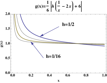
Figure 1: $g(x)>h$, for $h=1/2,1/4,1/8,1/16$.

For $h=1/2$, we have

$$\begin{array}[]{ll}I(f)&=0.746824\\ Q_{3}(f)&=2\,h\,f(0)=1\\ \tilde{E}_{3}(f)&=2h^{2}f[0,1/2]+\displaystyle{\frac{2\,h^{3}}{3}}\,f[0,1/2,1]=\\ &=-0.221199-0.03162046=-0.252850\\ S_{3}(f)&=Q_{3}(f)+\tilde{E}_{3}(f)=0.747180.\\ \end{array}$$

$$\begin{array}[]{ | c | c | c| }\hline\cr h&\bar{E}_{S_{3}}(f)=\displaystyle{\frac{-2\,h^{3}}{15}\frac{f[x_{1},x_{2},x_{3},\bar{x}_{1},\bar{x}_{2}]}{f[x_{1},x_{2}]}}\times\tilde{E}_{3}(f)&E_{S_{3}}(f)=I(f)-S_{3}(f)\\ \hline\cr 1/2&-0.000396282&-0.000356296\\ \hline\cr 1/4&-0.000115228&-0.0000900798\\ \hline\cr 1/8&-4.92044\times 10^{-6}&-3.72994\times 10^{-6}\\ \hline\cr 1/16&-1.65494\times 10^{-7}&-1.24455\times 10^{-7}\\ \hline\cr\end{array}$$

Table 3: Realistic and true error for $S_{3}(f)$.

Example 3.3.

(A realistic error for the $S_{5}(f)$ rule)

From Table 1 we obtain the following expression for the rule $S_{5}(f)$,

$$S_{5}(f)=4\,h\,f(x_{1})+\left\{8\,h^{2}f[x_{1},x_{2}]+\frac{40}{3}\,h^{3}\,f[x_{1},x_{2},x_{3}]+16\,h^{4}\,f[x_{1},\ldots,x_{4}]\right\}.$$ (41)

Consider $I(f)=\int_{0}^{4\,h}sin(2\,x)dx=sin^{2}(4\,h)$ and the interval $J=[a,b]=[0,\pi/5]$. Since $f\in C^{6}(J)$ and $f^{\prime}(x)=2\,\cos(2\,x)\neq 0,\,\,\forall\,x\in J$, the condition (25) holds with $x_{1}=0$ and $x_{5}=4\,h$. Let

$$\begin{array}[]{ll}g(x,h)&=\left|1+\displaystyle{\frac{a_{3}\,f^{(2)}(x)}{a_{2}\,2!\,f^{\prime}(x)}}+\displaystyle{\frac{a_{4}\,f^{(3)}(x)}{a_{2}\,3!\,f^{\prime}(x)}}+\displaystyle{\frac{a_{5}\,f^{(4)}(x)}{a_{2}\,4!\,f^{\prime}(x)}}\right|,\qquad a<x<b\\ &=\left|1-\displaystyle{\frac{4\,h^{2}}{3}}+\displaystyle{\frac{1}{45}(14\,h^{2}-75)\,h\,\tan(2x)}\right|,\end{array}$$

where the coefficients $a_{i}$ are computed using (15). It can be observed in the plot in the Figure 2 that for $h\in\{1/8,1/16,1/32,1/64\}$ the condition $g(x,h)>h$ is satisfied. Therefore, since $n$ is odd, one concludes from Proposition 3.1 (a) that the following realistic estimation for the true error of $S_{5}(f)$ is,

$$\begin{array}[]{ll}\bar{E}_{S_{5}}(f)&=\displaystyle{\frac{I(w_{6})}{I(w_{1})}\frac{f[x_{1},x_{2},\ldots,x_{5},\bar{x}_{1},\bar{x}_{2}]}{f[x_{1},x_{2}]}}\times\tilde{E}_{5}(f)\\ &=\displaystyle{\frac{-16\,h^{5}}{21}\frac{f[x_{1},x_{2},\ldots,x_{5},\bar{x}_{1},\bar{x}_{2}]}{f[x_{1},x_{2}]}}\times\tilde{E}_{5}(f),\end{array}$$ (42)

where $\bar{x}_{1}=(x_{1}+x_{2})/2$ and $\bar{x}_{2}=(x_{4}+x_{5})/2$. In Table 4 are displayed the computed realistic errors $\bar{E}_{S_{5}}(f)$ for the steps $h$ referred above.

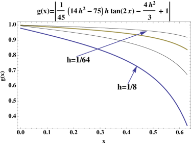
Figure 2: $g(x,h)>h$, for $h=1/8,1/16,1/32,1/64$.

For instance for $h=1/8$, we have

$$\begin{array}[]{ll}I(f)&=I=0.2298488470659301\\ Q_{5}(f)&=4\,h\,f(x_{1})=0\\ \\ \tilde{E}_{5}(f)&=8\,h^{2}f[x_{1},x_{2}]+\frac{40}{3}\,h^{3}f[x_{1},x_{2},x_{3}]+16h^{4}f[x_{1},\ldots,x_{4}]+\frac{112}{15}h^{5}f[x_{1},\ldots,x_{5}]=\\ &=0.2474039592545229-0.01281864992070238-\\ &-0.004808659341902015+0.00007207430695446034\\ &=0.2298487242988730,\end{array}$$

and finally

$$S_{5}(f)=Q_{5}(f)+\tilde{E}_{5}(f)=0.229848724298873.$$

$$\begin{array}[]{ | c | c | c| }\hline\cr h&\bar{E}_{S_{5}}(f)\simeq\displaystyle{\frac{-16\,h^{5}}{21}\frac{f[x_{1},x_{2},x_{3},x_{4},x_{5},\bar{x}_{1},\bar{x}_{2}]}{f[x_{1},x_{2}]}}\times\tilde{E}_{5}(f)&E_{S_{5}}(f)=I(f)-S_{5}f)\\ \hline\cr 1/8&1.14143\times 10^{-7}&1.22767\times 10^{-7}\\ \hline\cr 1/16&4.89318\times 10^{-10}&4.98246\times 10^{-10}\\ \hline\cr 1/32&1.95599\times 10^{-12}&1.96484\times 10^{-12}\\ \hline\cr 1/64&7.68478\times 10^{-15}&7.69335\times 10^{-15}\\ \hline\cr\end{array}$$

Table 4: Realistic and true error for $S_{5}(f)$.

4 Composite rules

The rules whose weights have been given in Table 1 are here applied in order to obtain the so-called composite rules. The algorithm described hereafter for composite rules is illustrated by several examples presented in paragraph 4.1. Since the best rules $S_{n}$ are the ones for which $n$ is even (when $deg(S_{n})=n$ holds) the examples refer to $S_{3}$, $S_{5}$, $S_{7}$ and $S_{9}$. Whenever the conditions of Proposition 3.1 for obtaining realistic errors are satisfied, these rules enable the computation of high precision approximations to the integral $I(f)$, as well as good approximations to the true error. This justifies the name realistic error adopted in this work.

Let $n\geq 2$ be given and fix a natural number $i$. Consider the number $N=(n-1)\times i$ and divide the interval $[a,b]$ into $N$ equal parts of length $h=(b-a)/N$, denoting by $x_{1},x_{2},\ldots,x_{N}$ the nodes, with $x_{1}=a$, $x_{N}=b$, and $x_{j}=x_{j-1}+h,\quad j=2,3,\ldots(N-1)$. Partitioning the set $\{x_{1},x_{2},\ldots,x_{N}\}$ into subsets of $n$ points each, and for an offset of $n-1$ points, we get $i$ panels each one containing $n$ successive nodes. To each panel we apply in succession the rule $Q_{n}$ and compute the respective realistic correction $\tilde{E}_{n}$ as well as the estimated realistic error $\bar{E}_{S_{n}}$ for the rule $S_{n}(f)$. For the output we compute the sum of the partial results obtained for each panel as described in (43):

$$\left\{\begin{array}[]{l}Q=\sum_{k=1}^{i}Q_{n}(\mbox{panel}_{k})\\ \tilde{E}=\sum_{k=1}^{i}\tilde{E}_{n}(\mbox{panel}_{k})\\ S=Q+\tilde{E}\quad\mbox{(composite rule)}\\ \bar{E}=\sum_{k=1}^{i}\bar{E}_{n}(\mbox{panel}_{k})\quad\mbox{(realistic error for $S$)}.\end{array}\right.$$ (43)

According to Proposition 2.4, for composite rules with $n$ points by panel and step $h>0$, in the favorable cases (those satisfying the hypotheses behind the theory) one can expect to be able to compute approximations $S$ having a realistic error. Analytic proofs for realistic errors in composite rules for both models $A$ and $B$ will be treated in a forthcoming work [3].

4.1 Numerical examples for composite rules

Once computed realistic errors within each panel for a composite rule, we can expect the error $\bar{E}$ in (43) to be also realistic. This happens in all the numerical examples worked below.

Example 4.1.

Let

$$\begin{array}[]{ll}I(f)&=\int_{10^{5}}^{2\times 10^{5}}\displaystyle{\frac{1}{\ln(x)}}dx\qquad\mbox{(\cite[cite]{[\@@bibref{}{steffensen}{}{}]}, p. 161 )}\\ &=li(2\times 10^{5})-li(10^{5})\end{array}$$

In the interval $J=[10^{5},2\times 10^{5}]$, the function $f(x)=1/\ln(x)$ belongs to the class $C^{\infty}(J)$. Since $f^{\prime}(x)=-(x\,\ln^{2}(x))^{-1}\neq 0$, for all $x\in J$, and for $k\geq 2$ the quotients $f^{(k)}(x)/f^{\prime}(x)$, with $x\in J$, are close to $\gamma(x)=0$ and tends to the zero function $\gamma(x)$ as $k$ increases. Therefore, the lefthand side in the inequality (26) is very close to $1$. That is, for $n\geq 2$ the function

$$g(x,h)=\left|1+\sum_{j=2}^{n-1}\displaystyle{\frac{a_{j+1}}{a_{2}}}\,\displaystyle{\frac{f^{(j)}(x)}{j!\,f^{\prime}(x)}}\right|$$

is such that $g(x,h)\simeq 1$, for $h$ sufficiently small. So Proposition 3.1 holds and one obtains realistic errors for the rules $S_{n}(f)$.

The behavior of the function $g(x,h)$ is illustrated for the case $n=3$ in Figure 3, for $h\,\in\{5,5/2,5/3\}$. Note that in this example $g(x)\simeq 1$ while the chosen steps $h$ are greater than $1$. However, realistic errors are still obtained.

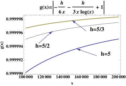
Figure 3: $n=3$. $g(x)\simeq 1$, for $h=5,5/2,5/3$.

Using a precison of $32$ decimal digits (or greater for $n>3$) the following values are obtained for the $3$-point composite rule:

$$\begin{array}[]{ll}I&=8406.2431208462027086216460436947\\ h&=5\\ Q&=8406.2677835091928175\\ E&=-0.024662837510842808609+1.7452073401705812569\times 10^{-7}=\\ &=-0.024662662990108791550\\ S&=8406.2431208462027087\\ \bar{E}_{S}&=-5.9854000\times 10^{-17}\quad\mbox{ (realistic error for $S$) }\\ I-S&=-5.9854472*10^{-17}\quad\mbox{(true error)}.\end{array}$$

In Table 5 the realistic error is compared with the true error, respectively for the rules with $n$ odd from $3$ to $9$ points (the step $h$ is as tabulated).

$$\begin{array}[]{|c|c|c| c|}\hline\cr n&h&\bar{E}_{S}&I-S\\ \hline\cr 3&5&-5.98540\times 10^{-17}&-5.98545\times 10^{-17}\\ \hline\cr 3&5/3&-7.38942\times 10^{-19}&-7.38944\times 10^{-19}\\ \hline\cr 5&5/2&-1.30573\times 10^{-26}&-1.30576\times 10^{-26}\\ \hline\cr 5&5/6&-1.79116\times 10^{-29}&-1.79117\times 10^{-29}\\ \hline\cr 7&5/3&-5.31897\times 10^{-36}&-5.31911\times 10^{-36}\\ \hline\cr 7&5/6&-2.07775\times 10^{-38}&-2.07778\times 10^{-38}\\ \hline\cr 9&25/6&-4.95560\times 10^{-40}&-4.95608\times 10^{-40}\\ \hline\cr 9&5/2&-2.99658\times 10^{-42}&-2.99675\times 10^{-42}\\ \hline\cr\end{array}$$

Table 5: Comparison of the realistic error $\bar{E}_{S}$ with the true error.

For $n=7$, the computed approximation for the integral $I$ is

$$S=8406.24312084620270862164604369467068,$$

where all the digits are correct. The simple rule $S_{7}(f)$ is defined (see Table 1) as

$$\begin{array}[]{ll}S_{7}(f)&=6\,h\,f(x_{1})+\left\{18h^{2}f[x_{1},x_{2}]+54h^{3}f[x_{1},x_{2},x_{3}]+144h^{4}f[x_{1},\ldots,x_{4}]+\right.\\ &+\left.\frac{1476}{5}h^{5}f[x_{1},\ldots,x_{5}]+396h^{6}f[x_{1},\ldots,x_{6}]+\frac{1476}{5}f[x_{1},\ldots,x_{7}]\right\}.\end{array}$$ (44)

The respective realistic error is (see (27))

$$\bar{E}_{S_{7}}=\frac{I(w_{8})}{i(w_{1})}\frac{d_{8}}{d_{1}}\times\tilde{E}_{7}=-\frac{72}{5}\,h^{7}\frac{d_{8}}{d_{1}}\times\tilde{E}_{7}.$$ (45)

In Appendix 4.1 a Mathematica code for the composite rule $S$, for $n=7$, is given. The respective procedure is called $Q7A$ and the code includes comments explaining the respective algorithm. Of course we could have adopted a more efficient programming style, but our goal here is simply to illustrate the algorithm described above for the composite rules.

Appendix 4.1.

(Composite rule $S$ for $n=7$ points )

$$\begin{array}[]{l}\mbox{(* For the data }\,\,\{x_{1},\ldots,x_{n}\},\,\{f_{1},\ldots,f_{n}\},\,\,\mbox{and}\,\,k\geq 0\\ \mbox{ the output for $d[x,y,k,p]$ is the divide difference}\,f[x_{1},\ldots,x_{k}]\,\,\mbox{*)}\\ \mbox{(* The user may enter a precision $p$ which will be assigned to the data. *)}\\ \mbox{(* By default $p=\infty$ *)}\\ \end{array}$$

$$\begin{array}[]{l}d[xi\verb+_+List,yi\verb+_+List,k\verb+_+/;k>=0,precision\verb+_+:Infinity]:=\\ Module[\{n=Length[xi],x,y,dd\},\\ \hskip 85.35826pt\mbox{(* set default precision to nodes xi *)}\\ x=SetPrecision[xi,precision];\\ \hskip 85.35826pt\mbox{ (* set default precision to functional values yi *)}\\ y=SetPrecision[yi,precision];\\ \mbox{ (* recursive definiton for finite differences : *) }\\ \end{array}$$

$$\begin{array}[]{l}dd[0,j\verb+_+]:=y[[j]];\mbox{ (* order 0 difference *) }\\ \mbox{ (* ordem i difference; dynamic computation *) }\\ dd[i\verb+_+,j\verb+_+]:=dd[i,j]=(dd[i-1,j+1]-dd[i-1,j])/(x[[i+j]]-x[[j]]);\\ \mbox{ (* Output: first difference of order k *) }\\ dd[k,1]\quad];\\ \end{array}$$

$$\begin{array}[]{l}\mbox{(* The procedure $q7A$ uses the algorithm for the simple rule with n=7}\\ \hskip 142.26378pt\mbox{ nodes *) }\\ \mbox{(* The output is a list containing the relevant items for this simple rule *)}\\ \\ q7A[\{\{t1\verb+_+,f1\verb+_+\},\{t2\verb+_+,f2\verb+_+\},\{t3\verb+_+,f3\verb+_+\},\{t4\verb+_+,f4\verb+_+\},\{t5\verb+_+,f5\verb+_+\},\{t6\verb+_+,f6\verb+_+\},\\ \hskip 142.26378pt\{t7\verb+_+,f7\verb+_+\}\},precision\verb+_+:Infinity]:=\\ Module[\{x1,x2,x3,x4,x5,x6,x7,xb1,xb2,y1,y2,y3,y4,y5,y6,y7,\\ \hskip 85.35826ptyext,hh,ext,d1,d8,q,e1,e2,e3,e4,e5,e6,E7,s,real\},\\ \end{array}$$

$$\begin{array}[]{l}\{y1,y2,y3,y4,y5,y6,y7\}=SetPrecision[\{f1,f2,f3,f4,f5,f6,f7\},\\ \hskip 142.26378ptprecision];\\ \{x1,x2,x3,x4,x5,x6,x7\}=SetPrecision[\{t1,t2,t3,t4,t5,t6,t7\},\\ \hskip 142.26378ptprecision];\\ xb1=(x1+x2)/2;xb2=(x6+x7)/2;\\ ext=\{x1,x2,x3,x4,x5,x6,x7,xb1,xb2\};\\ yext=Map[f,ext];\quad\mbox{(* completation of the panel *) }\\ d1=d[\{x1,x2\},\{y1,y2\},1];\quad\mbox{(* divided difference order 1 *)}\\ \end{array}$$

$$\begin{array}[]{l}d8=d[ext,yext,8,precision];\quad\mbox{(* divided difference order 8 *)}\\ hh=SetPrecision[h,precision];\quad\mbox{ (* step *)}\\ q=6*hh*y1;\quad\mbox{ (* left rectangle quadrature rule *) }\\ e1=18*hh^{2}*d[\{x1,x2\},\{y1,y2\},1];\quad\mbox{ (* error e1 *)}\\ e2=54*hh^{3}*d[\{x1,x2,x3\},\{y1,y2,y3\},2];\quad\mbox{ (* error e2 *) }\\ \hskip 142.26378pt\mbox{ (* error e3 : *) }\\ e3=144*hh^{4}*d[\{x1,x2,x3,x4\},\{y1,y2,y3,y4\},3];\\ \hskip 142.26378pt\mbox{ (* error e4 : *) }\\ e4=1476/5*hh^{5}*d[\{x1,x2,x3,x4,x5\},\{y1,y2,y3,y4,y5\},4];\\ \hskip 142.26378pt\mbox{ (* error e5 : *) }\\ e5=396*hh^{6}*d[\{x1,x2,x3,x4,x5,x6\},\{y1,y2,y3,y4,y5,y6\},5];\\ \hskip 142.26378pt\mbox{ (* error e6 : *) }\\ e6=1476*hh^{7}/7*d[\{x1,x2,x3,x4,x5,x6,x7\},\\ \hskip 142.26378pt\{y1,y2,y3,y4,y5,y6,y7\},6];\\ E7=e1+e2+e3+e4+e5+e6;\quad\mbox{ (* realistic error for q *)}\\ s=q+E7;\quad\mbox{ (* s is a realistic approximation to the integral *) }\\ \end{array}$$

$$\begin{array}[]{l}real=N[-72*hh^{7}/5*d8/d1*E7,8];\quad\mbox{ (* realistic error for s *) }\\ \{q,e1,e2,e3,e4,e5,e6,E7,s,real\}];\quad\mbox{ (* output *)}\end{array}$$

$$\begin{array}[]{l}\mbox{(* The following procedure $Q7A$ gives a list containing the relevant }\\ \hskip 56.9055pt\mbox{ items for the composite rule. It calls the procedure $q7A$: *)}\\ \\ Q7A[x\verb+_+List,y\verb+_+List,precision\verb+_+:Infinity]:=Module[\{data,list\},\\ \hskip 56.9055pt\mbox{ (* partition into 7 nodes offset 6 *) }\\ data=Partition[Transpose[\{x,y\}],7,6];\\ \hskip 71.13188pt\quad\mbox{ (* sum entries in cells and prepend the step h used *)}\\ list=Map[q7A[\verb+#+,precision]\verb+&+,data];\\ Prepend[Map[Apply[Plus,\verb+ #+]\verb+&+,Transpose[list]],Rationalize[h]]\,\,];\\ \end{array}$$

Acknowledgments

This work has been supported by Instituto de Mecânica-IDMEC/IST, Centro de Projecto Mecânico, through FCT (Portugal)/program POCTI.

References

- [1] P. J. Davis and P. Rabinowitz, Methods of Numerical Integration, Academic Press, Orlando, 1984.
- [2] W. Gautschi, Numerical Analysis, An Introduction, Birkhauser, Boston, 1997.
- [3] M. M. Graça, Realistic errors for corrected open Newton-Cotes rules, In preparation.
- [4] E. Isaacson and H. B. Keller, Analysis of numerical methods, John Wiley & Sons, New York, 1966.
- [5] V. I. Krylov, Approximate Calculation of Integrals, Dover, New York, 2005.
- [6] J. F. Steffensen, Interpolation, Dover, 2nd Ed., Boston, 2006.