Scalar and electromagnetic fields of static sources in higher dimensional Majumdar-Papapetrou spacetimes

Abstract

We study massless scalar and electromagnetic fields from static sources in a static higher dimensional spacetime. Exact expressions for static Green’s functions for such problems are obtained in the background of the Majumdar-Papapetrou solutions of the Einstein-Maxwell equations. Using this result we calculate the force between two scalar or electric charges in the presence of one or several extremally charged black holes in equilibrium in the higher dimensional spacetime.

I Introduction

There exists a variety of interesting physical problems that require study of a test electromagnetic field in a curved spacetime. For such problems one uses a test field approximation: The field propagates in a fixed gravitational background and its backreaction on the metric is neglected. This approximation is often used for the study of electric and magnetic fields created by sources near a black hole. Black hole electrodynamics is an important part of the membrane paradigm MEMPAR and has important applications in black hole astrophysics.

In the present paper we consider the static field of a pointlike charge placed in the black hole vicinity. In a local frame such a field close to the charge is radial and similar to the field of a charge in a flat space. However the action of gravity modifies the field at far distance from the charge. This modification can be easily ‘explained’ as the gravitational attraction of the energy-stress distribution associated with the test field.

The simplest case is a situation when an electric charge is at rest in a uniform gravitational field. The corresponding electric field can be easily obtained by writing the corresponding Liénard-Wiechert potential for a uniformly accelerated charge in the Rindler coordinates. In 1921 Fermi fermi used this approach to study how the homogeneous gravitational field affects the self-energy of an electric charge. A similar problem of the self energy for charged particles at rest in the vicinity of a neutral and charged black holes was discussed more recently in SmithWill:1980 ; FrolovZelnikov:1982 ; Lohiya:1982 ; ChoTsokarosWisseman:2007 . The remarkable fact is that the solutions for scalar massless and electric field created by a pointlike charge in the Schwarzschild and Reissner-Nordström metrics can be obtained in an explicit analytical form Copson:1928 ; LL ; Linet:1976 ; Linet:1977 . This result is a consequence of the generic property of these four dimensional metrics: They can be written in the form of the Weyl metric. If the axis of the symmetry is chosen so that it passes through the position of the charge, the corresponding equations for the static field for such a source are effectively reduced to the equations in a flat 3D space. Gibbons and Warnick GibbonsWarnick:2009 demonstrated that the exact static scalar and electromagnetic Green functions in the four-dimensional Schwarzschild and Reissner-Nordström spacetimes can be also obtained by reducing the problem to calculations in optical metrics. Unfortunately such methods do not work for higher dimensional generalizations of the spherically symmetric black holes. However recently Linet Linet:05 obtained explicit exact solutions for the field of a pointlike particle in the vicinity of higher dimensional extremally charged Reissner-Nordström black hole.

In this paper we obtain exact solution of this problem in a wide class of physically interesting metrics and provide a far going generalization of Linet’s results.

The aim of this paper is to demonstrate that in the higher dimensional case there exist wide class of physically interesting metrics where the massless scalar and electric field equations allow exact solutions for pointlike charges. This class includes so called Majumdar-Papapetrou solutions of the Einstein-Maxwell equations. The corresponding solutions describe one or several extremally charged higher dimensional black holes in equilibrium. They are supersymmetric and saturate the Bogomol’nyi bound. These solutions are widely discussed in the string theory (see e.g. Ortin ; Maeda ). The $D-$dimensional Majumdar-Papapetrou solution is static and its spatial part is conformal to the $(D-1)-$dimensional Euclidean metric. We demonstrate that this property allows one to reduce static scalar and electric problems to similar problems in a flat space.

The paper is organized as follows. In Section 2 we recall some properties of the Majumdar-Papapetrou solutions and discuss two special cases: a single higher dimensional extremal Reissner-Nordström black hole, and such a black hole in a space with compact extra dimension. This material is well known. We collect here the results, basically in order to fix notations we use in the main text. In Sections 3 and 4 we obtain explicit expressions for scalar and electric field of a point charge in the Majumdar-Papapetrou geometry. We also analyze interesting special cases and discuss how the presence of extremally charged black holes modifies the interaction force between charges in these spacetimes.

II Majumdar-Papapetrou solutions of Einstein-Maxwell equations

II.1 General form of the Majumdar-Papapetrou metric

The higher dimensional Einstein-Maxwell action is

$$\begin{split}S&=S_{\mbox{\tiny g}}+S_{\mbox{\tiny em}}\,,\\ S_{\mbox{\tiny g}}&={1\over 16\pi G^{(D)}}\int d^{D}x\sqrt{-g}\,R,\\ S_{\mbox{\tiny em}}&=-{1\over 16\pi}\int d^{D}x\sqrt{-g}\,F_{\mu\nu}F^{\mu\nu}+\int d^{D}x\sqrt{-g}\,A_{\mu}J^{\mu}\,.\end{split}$$ (1)

In $D=n+3$ dimensions the solution which describes the metric of a set of extremally charged black holes at rest can be written in the form

$$ds^{2}=-U^{-2}\,dt^{2}+U^{2/n}\delta_{ab}\,dx^{a}dx^{b}\,.$$ (2)

The corresponding static electric field is given by the vector potential

$${\cal A}_{\mu}=\sqrt{{n+1\over 2n}}\,U^{-1}\,\delta^{0}_{\mu}\,.$$ (3)

This is an exact solution of the Einstein-Maxwell equations if the function $U$ satisfies the equation

$$\bigtriangleup U=0\,,$$ (4)

that is, it is a harmonic function. We denote by Greek indices the spacetime coordinates and use Latin indices $a,b,\dots$ or bold face fonts for spatial coordinates $x^{\mu}\equiv(t,x^{a})\equiv(t,\boldsymbol{x})$. The $(n+2)-$dimensional Laplacian in Eq.(4) is defined in accordance to the flat spatial metric

$$\bigtriangleup\equiv\delta^{ab}\partial_{a}\partial_{b}\,.$$ (5)

We also use here the flat metric to define the norm of the spatial vector

$$|\boldsymbol{x}|\equiv\sqrt{\delta_{ab}\,x^{a}x^{b}}\,.$$ (6)

The ‘coordinate distance’ between spatial points $\boldsymbol{x}$ and $\boldsymbol{x}^{\prime}$ then reads $|\boldsymbol{x}-\boldsymbol{x}^{\prime}|$ .

For a special choice of the solution

$$U=1+\sum_{k}{M_{k}\over\rho_{k}^{n}}\,,\hskip 17.07182pt\rho_{k}=|\boldsymbol{x}-\boldsymbol{x}_{k}|\,,$$ (7)

the metric Eq.(2) describes multiple black holes in equilibrium, when the gravitational attraction between them is exactly compensated by the electromagnetic repulsion. These metrics are the higher dimensional generalization Myers:1986 of the Majumdar-Papapetrou metrics. The metric with $k=1,\ldots,N$ describes $N$ extremally charged black holes in a static equilibrium. Here $\boldsymbol{x}_{k}$ is the spatial position of the $k$-th extremal black hole. The function $U$ obeys the homogeneous equation Eq.(4) everywhere outside these points. When these points are included one has

$$\bigtriangleup U=-{4\pi^{1+{n\over 2}}\over\Gamma\left({n\over 2}\right)}\sum_{k}M_{k}\,\delta^{n+2}(\boldsymbol{x}-\boldsymbol{x}_{k})\,.$$ (8)

These $\delta-$functions are localized on the horizons. They correspond to the effective charge distributions

$$\begin{split}\sqrt{-g}\,{\cal J}^{0}&=-\sqrt{n+1\over 2n}{\bigtriangleup U\over 4\pi}\\ &=\sqrt{n+1\over 2n}{\pi^{n\over 2}\over\Gamma\left({n\over 2}\right)}\sum_{k}M_{k}\,\delta^{n+2}(\boldsymbol{x}-\boldsymbol{x}_{k})\,.\end{split}$$ (9)

on the horizons of the charged black holes of the Majumdar-Papapetrou spacetime.

II.2 Special cases

II.2.1 Higher dimensional extremal Reissner-Nordström black hole

A simplest case of the Majumdar-Papapetrou metric is an an extremal Reissner-Nordström black hole

$$\begin{split}ds^{2}&=-U^{-2}\,dt^{2}+U^{2/n}\,dr^{2}+r^{2}\,d\Omega_{n+1}^{2}\,,\\ U&=\left(1-{r_{{\mbox{\tiny g}}}^{n}\over r^{n}}\right)^{-1}\,.\end{split}$$ (10)

Here $r_{{\mbox{\tiny g}}}$ is the gravitational radius of the black hole and $d\Omega_{n+1}^{2}$ is the metric on a unit $(n+1)$-dimensional sphere

$$d\Omega_{n+1}^{2}=d\theta_{n+1}^{2}+\sin^{2}\theta_{n+1}d\Omega_{n}^{2}\,.$$ (11)

We shall use notations

$$\theta=\theta_{n+1}\,,\hskip 17.07182pt\phi=\theta_{1}\,.$$ (12)

The angles $\theta_{j>1}$ change in the interval $(0,\pi)$, while $\phi$ changes in the interval $(0,2\pi)$.

The vector potential ${\cal A}_{\mu}$ of the electric field is

$${\cal A}_{\mu}=\sqrt{{n+1\over 2n}}\,\left(1-{r_{{\mbox{\tiny g}}}^{n}\over r^{n}}\right)\,\delta^{0}_{\mu}\,.$$ (13)

At infinity the potential does not vanish but asymptotically approaches a pure gauge solution.

After the coordinate transformation

$$\rho^{n}=r^{n}-r_{{\mbox{\tiny g}}}^{n}$$ (14)

the Reissner-Nordström metric takes the form, where the spatial part is conformally flat

$$\begin{split}ds^{2}&=-U^{-2}\,dt^{2}+U^{2/n}\,\left(d\rho^{2}+\rho^{2}\,d\Omega_{n+1}^{2}\right)\,,\\ U&=1+{r_{{\mbox{\tiny g}}}^{n}\over\rho^{n}}\,.\end{split}$$ (15)

In this particular case of a single black hole these coordinated are called isotropic. It is convenient to introduce the ‘coordinate distance’ between two points in the metric Eq.(15) which is just the distance defined by the flat spatial geometry $R(\boldsymbol{x},\boldsymbol{x^{\prime}})=|\boldsymbol{x}-\boldsymbol{x^{\prime}}|$ (see Eq.(6)).

II.2.2 Compactified extremally charged black hole

The Majumdar-Papapetrou metric Eq.(2) can be used for description of a spacetime of a single black hole but in a compactified spacetime with the spatial topology of a cylinder Myers:1986 . The idea is simple. Consider at first a black hole in the space with the topology of a cylinder and which is periodic in one direction, e.g., $L^{a}$ with the coordinate period $L=|\boldsymbol{L}|$. This spacetime is equivalent to the multi black hole metric where all black holes are aligned in one direction with an equal distance between them and have the same masses. This is evidently a particular case of the generic higher dimensional Majumdar-Papapetrou metric with the function

$$U(\boldsymbol{x})=1+M\sum_{k=-\infty}^{\infty}{1\over\rho_{k}^{n}}\,,\hskip 17.07182pt\rho_{k}=|\boldsymbol{x}-\boldsymbol{x}_{\mbox{\tiny BH}}-k\boldsymbol{L}|\,.$$ (16)

Without loss of generality one can always put the black hole in the coordinate origin $\boldsymbol{x}_{\mbox{\tiny BH}}=0$, and choose $L^{a}=(0,\dots,0,L)$. Then

$$\begin{split}\rho_{k}&=\sqrt{[(z-kL)^{2}+\ell^{2}]}\,,\hskip 17.07182ptz\equiv x^{n+2}\,,\\ \ell^{2}&\equiv\delta_{ij}x^{i}x^{j}\,,\hskip 17.07182pti,j=(1,\dots,n+1)\,.\end{split}$$ (17)

For example in five dimensions $(n=2)$ the summation leads to

$$U(\boldsymbol{x})=1+M\,{\pi\over\ell L}\,{\sinh{(2\pi\ell/L)}\over\cosh{(2\pi\ell/L)}-\cos{(2\pi z/L)}}\,.$$ (18)

In any odd dimensions one can easily derive a more complicated but similar expression in terms of elementary functions. Namely, if $j=n/2$ is integer then

$$U(\boldsymbol{x})=1-M\,{(-1)^{j}\over j!}\,\left({1\over 2\ell}{\partial\over\partial\ell}\right)^{j}\left[\ln\left(\cosh{2\pi\ell\over L}-\cos{2\pi z\over L}\right)\right]\,.$$ (19)

In even dimensions (odd $n$) there is no simple expression for this sum.

III Static massless scalar field in Majumdar-Papapetrou spacetimes

III.1 Massless scalar field with sources

The best way to deal with this problem is to start with the total action for the particles carrying a scalar charge. It consists of the scalar field action, the action of the massive particle itself, and the interaction term

$$\begin{split}S&=S_{\mbox{\tiny sc}}+S_{\mbox{\tiny m}}+S_{\mbox{\tiny int}}\,,\\ S_{\mbox{\tiny sc}}&=-{1\over 8\pi}\int d^{D}x\sqrt{-g}\,\varphi^{;\mu}\varphi_{;\mu}\,,\\ S_{\mbox{\tiny m}}&=-\int d\tau\,m\sqrt{-u^{\mu}u_{\mu}}\,,\\ S_{\mbox{\tiny int}}&=\int d^{D}x\,\sqrt{-g}\,\varphi(x)J(x)\,.\end{split}$$ (20)

Consider two pointlike scalar charges $q$ and $q^{\prime}$ located at points $\boldsymbol{y}$ and $\boldsymbol{y^{\prime}}$, respectively, in the spacetime with the metric Eq.(2). The source describing a pointlike scalar charge moving along the worldline $y^{\mu}(\tau)$ is

$$\begin{split}J(x)=q\,\int d\tau\,\sqrt{-u^{\mu}u_{\mu}}\,\delta^{D}(x^{\mu},{y}^{\mu})\,,\end{split}$$ (21)

where $\tau$ is its proper time and $\delta^{D}(x^{\mu},{y}^{\mu})=(-g)^{-1/2}\delta^{D}(x^{\mu}-{y}^{\mu})$ is the covariant D-dimensional $\delta$-function $(D=n+3)$. In this expression the factor $\sqrt{-u^{\mu}u_{\mu}}$ is equal to 1 on the equations of motion, but for an arbitrary off-shell trajectory it is to be considered a functional of the path. This factor is necessary for the consistency of the variation procedure. In order to calculate the force exerted by one scalar charge to another, one has to keep in mind peculiar properties of the scalar field.

Variation of this action over the particle path gives the equation of motion. For a particle of mass $m$ and a scalar charge $q$ we obtain

$${d\over d\tau}p_{\mu}=f_{\mu}.$$ (22)

Here

$$p_{\mu}=(m-q\phi)\,u_{\mu}$$ (23)

is the canonical momentum of the scalar particle. The tricky point is that the effective inertial mass of the scalar charge depends on the scalar field ChiuHoffmann:1964

$$m_{\mbox{\tiny eff}}=m-q\varphi(y)$$ (24)

and, hence, is not constant in spacetime because in a general case the scalar field $\varphi$ is not homogeneous. The force acting on the scalar charge is

$$f_{\mu}=q\,\varphi_{;\mu}\,.$$ (25)

If the scalar field $\varphi$ is created by another static pointlike charge $q^{\prime}$ located at the spatial point $\boldsymbol{y}^{\prime}$

$$\begin{split}J^{\prime}(\boldsymbol{x})&=q^{\prime}\,{\sqrt{-g_{00}(\boldsymbol{x})}\over\sqrt{-g(\boldsymbol{x})}}\,\delta^{n+2}(\boldsymbol{x}-{\boldsymbol{y}^{\prime}})\\ &=q\,U^{-1-{2\over n}}(\boldsymbol{x})\,\delta^{n+2}(\boldsymbol{x}-{\boldsymbol{y}^{\prime}}).\end{split}$$ (26)

then it can be expressed in terms of the Green function

$$\varphi(\boldsymbol{y})=4\pi q^{\prime}\,\sqrt{-g_{00}(\boldsymbol{y}^{\prime})}\,{\cal G}(\boldsymbol{y},{\boldsymbol{y}^{\prime}})\,.$$ (27)

III.2 Field of a scalar point charge

Let us consider a pointlike scalar charge in a $(n+3)-$dimensional static spacetime with the metric

$$ds^{2}=-U^{2}dt^{2}+H^{2}dl^{2}\,.$$ (28)

Here $dl^{2}$ is a flat $(n+2)-$dimensional metric

$$dl^{2}=\delta_{ab}dx^{a}dx^{b}\,,\hskip 17.07182pta,b=1,\ldots,n+2\,,$$ (29)

and $U$ and $H$ are functions of spatial coordinates $x^{a}$. The massless scalar field equation is of the form

$$\Box\varphi=-4\pi J\,,\hskip 17.07182pt\Box\equiv g^{\mu\nu}\nabla_{\mu}\nabla_{\nu}\,.$$ (30)

We focus our attention on a static field $\varphi$ generated by a static source $J$. It obeys the equation

$$\Delta^{(n+2)}\varphi=-4\pi J\,,$$ (31)

where

$$\Delta^{(n+2)}={U\over H^{n+2}}\delta^{ab}\partial_{a}\left(U^{-1}H^{n}\partial_{b}\right)\,.$$ (32)

For a special case of Majumdar-Papapetrou spacetime, when $H=U^{1/n}$ the operator $\Delta^{(n+2)}$ is proportional for the $(n+2)-$dimensional flat Laplace operator $\bigtriangleup=\delta^{ab}\partial_{a}\partial_{b}$ and the equation Eq.(31) takes the form

$$\bigtriangleup\varphi=-4\pi U^{2/n}J\,.$$ (33)

The metric Eq.(28) in this case takes the form Eq.(2).

The static Green function for $(n+2)-$dimensional Laplace operator is a solution of the equation

$$\bigtriangleup{\cal G}(\boldsymbol{x},\boldsymbol{x^{\prime}})=-\delta^{n+2}(\boldsymbol{x}-\boldsymbol{x^{\prime}})\,.$$ (34)

Using the following two relations

$$\bigtriangleup\left[{1\over\rho^{n}}\right]=-{4\pi^{1+{n\over 2}}\over\Gamma\left({n\over 2}\right)}\,\delta^{n+2}(\boldsymbol{x})=-n{1\over\rho^{n+1}}\,\delta(\rho)\,,$$ (35)

$$\delta^{n+2}(\boldsymbol{x})={\Gamma\left(1+{n\over 2}\right)\over 2\pi^{1+{n\over 2}}}\,{1\over\rho^{n+1}}\,\delta(\rho)\,,$$ (36)

one can easily obtain the Green function ${\cal G}(\boldsymbol{x},\boldsymbol{x^{\prime}})$

$${\cal G}(\boldsymbol{x},\boldsymbol{x^{\prime}})={\Gamma\left({n\over 2}\right)\over 4\pi^{1+{n\over 2}}}\,\cdot{1\over R^{n}}\,,$$ (37)

where

$$R(\boldsymbol{x},\boldsymbol{x^{\prime}})=|\boldsymbol{x}-\boldsymbol{x^{\prime}}|\,.$$ (38)

The function $R(\boldsymbol{x},\boldsymbol{x^{\prime}})$ is the coordinate distance Eq.(6) between points $\boldsymbol{x}$ and $\boldsymbol{x^{\prime}}$.

Therefore the solution for the scalar field corresponding to the generic static scalar source $J$ reads

$$\begin{split}\varphi(\boldsymbol{x})&=4\pi\int d^{n+2}x\,\sqrt{-g(\boldsymbol{x}^{\prime})}\,J(\boldsymbol{x}^{\prime})\,{\cal G}(\boldsymbol{x},\boldsymbol{x^{\prime}})\\ &=4\pi\int d^{n+2}x\,U^{2/n}(\boldsymbol{x}^{\prime})\,J(\boldsymbol{x}^{\prime})\,{\cal G}(\boldsymbol{x},\boldsymbol{x^{\prime}})\end{split}$$ (39)

III.3 Force between two pointlike scalar charges

Thus the force takes the form $f_{\mu}=(0,f_{a})$ where

$$f_{a}=-{n\,\Gamma\left({n\over 2}\right)\over\pi^{n\over 2}}\,{1\over U(\boldsymbol{y}^{\prime})}\,{qq^{\prime}\over R^{n+2}(\boldsymbol{y},\boldsymbol{y}^{\prime})}(y^{b}-y^{\prime}{}^{b})\,\delta_{ab}.$$ (40)

One can see that the force is attractive and $f^{a}\sim(y^{a}-y^{\prime}{}^{a})$, i.e., when written in the metric Eq.(2), it is directed exactly to the position of the charge $q^{\prime}$. The invariant absolute value of the force $|f|=\sqrt{f_{\mu}f^{\mu}}$ is

$$|f|={n\,\Gamma\left({n\over 2}\right)\over\pi^{n\over 2}}\,{1\over U^{1\over n}(\boldsymbol{y})U(\boldsymbol{y}^{\prime})}\,{qq^{\prime}\over R^{n+1}(\boldsymbol{y},\boldsymbol{y}^{\prime})}.$$ (41)

III.4 Special cases

III.4.1 Scalar field near higher dimensional extremally charged black hole

For a single black hole the higher dimensional Majumdar-Papapetrou metric Eq.(2) reduces to the higher dimensional version of the extremal Reissner-Nordström metric Eq.(15) in isotropic coordinates. In curvature coordinates it is given by Eq.(10) with the function

$$U=1+{r^{n}_{\mbox{\tiny g}}\over\rho^{n}}=\left(1-{r^{n}_{\mbox{\tiny g}}\over r^{n}}\right)^{-1}\,.$$ (42)

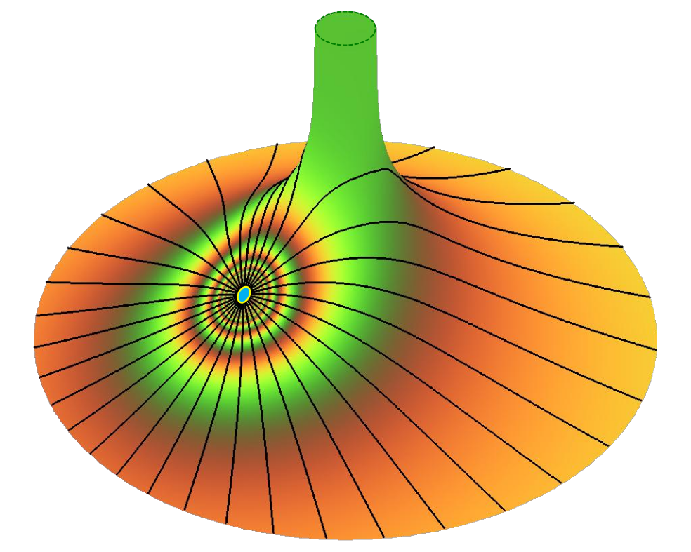
Figure 1: This figure depicts the scalar field force lines created by a charge in the extremal Reissner-Nordström black hole. The surface represents the embedding of the geometry of the equatorial section of the black hole to a three-dimensional flat space. Color function corresponds to the value of the scalar field $\varphi$, so that the lines of the same color would correspond to the equipotential lines. Near the charge the potential monotonically grows to infinity.

The static scalar Green function then reads

$${\cal G}(\boldsymbol{x},\boldsymbol{x^{\prime}})={\Gamma\left({n\over 2}\right)\over 4\pi^{1+{n\over 2}}}\,\cdot{1\over R^{n}}\,,$$ (43)

where the function $R$ in the isotropic spherical coordinates $(\rho,\boldsymbol{\theta})$ takes the form

$$\begin{split}R^{2}&=\rho^{2}+{\rho^{\prime}}^{2}-2\rho\rho^{\prime}\cos\lambda\,,\\ \cos\lambda&=\cos\theta\cos\theta^{\prime}+\sin\theta\sin\theta^{\prime}\,\cos\lambda_{n}\,,\\ \cos\lambda_{n}&=\cos\theta_{n}\cos\theta_{n}^{\prime}+\sin\theta_{n}\sin\theta_{n}^{\prime}\,\cos\lambda_{n-1}\,,\\ \theta_{1}&=\phi\,,\hskip 17.07182pt\theta_{n+1}=\theta\,,\hskip 17.07182pt\lambda_{n+1}=\lambda\,.\end{split}$$ (44)

The meaning of the functions $\lambda$ is the length of the arc of a great circle connecting two points $\boldsymbol{\theta}=(\theta_{1},\dots,\theta_{n},\theta)$ and $\boldsymbol{\theta^{\prime}}=(\theta^{\prime}_{1},\dots,\theta^{\prime}_{n},\theta^{\prime})$ on the surface of $n+1$-dimensional unit sphere. The same distance expressed in terms of the curvature coordinates $(r,\boldsymbol{\theta})$ (see Eq.(10)) reads

$$\begin{split}R^{2}&=\left(r^{n}-r_{{\mbox{\tiny g}}}^{n}\right)^{2/n}+\left({r^{\prime}}^{n}-r_{{\mbox{\tiny g}}}^{n}\right)^{2/n}\\ &-2\left(r^{n}-r_{{\mbox{\tiny g}}}^{n}\right)^{1/n}\left({r^{\prime}}^{n}-r_{{\mbox{\tiny g}}}^{n}\right)^{1/n}\cos\lambda\,,\\ \cos\lambda&=\cos\theta\cos\theta^{\prime}+\sin\theta\sin\theta^{\prime}\,\cos\lambda_{n}\,.\end{split}$$ (45)

If the charge $q^{\prime}$ is located at the point $\boldsymbol{x^{\prime}}$ then the corresponding scalar field is given by the formula Eq.(46)

$$\varphi(\boldsymbol{x})=4\pi q^{\prime}\,U^{-1}(\boldsymbol{x}^{\prime})\,{\cal G}(\boldsymbol{x},{\boldsymbol{x}^{\prime}})\,.$$ (46)

This special case reproduces the result by Linet Linet:05 for the scalar field near higher-dimensional extremal Reissner-Nordström black hole.

III.4.2 Scalar field in the spacetime of compactified extremally charged black hole

When written in the coordinates Eq.(2) the equation for the static Green function of the scalar field does not depend on the function $U$. Therefore, on a compact space one can independently derive the corresponding Green function ${\cal G}_{\mbox{\tiny(L)}}$ by a similar summation over images of a scalar charge

$${\cal G}_{{\mbox{\tiny(L)}}}(\boldsymbol{x},\boldsymbol{x^{\prime}})=\sum_{k=-\infty}^{\infty}{\cal G}(\boldsymbol{x},\boldsymbol{x^{\prime}}+k\boldsymbol{L})\,,$$ (47)

$${\cal G}_{\mbox{\tiny(L)}}(\boldsymbol{x},\boldsymbol{x^{\prime}})={\Gamma\left({n\over 2}\right)\over 4\pi^{1+{n\over 2}}}\,\cdot\sum_{k=-\infty}^{\infty}{1\over R_{k}^{n}}\,,$$ (48)

where

$$R_{k}(\boldsymbol{x},\boldsymbol{x^{\prime}})=|\boldsymbol{x}-\boldsymbol{x^{\prime}}-k\boldsymbol{L}|\,.$$ (49)

In 5D spacetime we get

$${\cal G}_{\mbox{\tiny(L)}}(\boldsymbol{x},\boldsymbol{x^{\prime}})={1\over 4\pi\,{\cal L}L}\,{\sinh{(2\pi{\cal L}/L)}\over\cosh{(2\pi{\cal L}/L)}-\cos{(2\pi(z-z^{\prime})/L)}}\,.$$ (50)

where

$$\begin{split}z&\equiv x^{n+2}\,,\hskip 17.07182ptz^{\prime}\equiv{x^{\prime}}^{n+2}\,,\hskip 17.07182pt\boldsymbol{L}=(0,\dots,0,L)\,,\\ {\cal L}^{2}&\equiv\delta_{ij}(x^{i}-{x^{\prime}}^{i})(x^{j}-{x^{\prime}}^{j})\,,\hskip 17.07182pti,j=(1,\dots,n+1)\,.\end{split}$$ (51)

IV Maxwell field of pointlike charge in Majumdar-Papapetrou spacetimes

IV.1 Reduction of the field equations

The Maxwell equations

$$F^{\mu\epsilon}{}_{;\epsilon}=4\pi J^{\mu}\,,\hskip 17.07182ptF_{\alpha\beta}=\nabla_{\alpha}A_{\beta}-\nabla_{\beta}A_{\alpha}\,,$$ (52)

for a static source $J^{\mu}=\delta^{\mu}_{0}J^{0}$ reduce to a single equation for the potential $A_{0}$

$${1\over\sqrt{-g}}\,\partial_{\epsilon}\left(\sqrt{-g}g^{00}g^{\epsilon\beta}\partial_{\beta}A_{0}\right)=-4\pi J^{0}\,,$$ (53)

or

$$\delta^{ab}\,\partial_{a}\left(U^{2}\partial_{b}A_{0}\right)=4\pi U^{2/n}\,J^{0}\,.$$ (54)

Substituting

$$A_{0}=-U^{-1}\psi\,,$$ (55)

we obtain

$$-\psi\bigtriangleup U+U\bigtriangleup\psi=-4\pi U^{2/n}\,J^{0}\,,$$ (56)

or

$$\left[\bigtriangleup-({U^{-1}\bigtriangleup U})\right]\psi=-4\pi U^{-1+{2\over n}}\,J^{0}\,.$$ (57)

For a point-like static source with the total charge $e^{\prime}=(4\pi)^{-1}$ located at the point $\boldsymbol{x^{\prime}}$

$$\sqrt{-g}\,J^{0}=U^{{2\over n}}\,J^{0}={1\over 4\pi}\,\delta^{n+2}(\boldsymbol{x}-\boldsymbol{x^{\prime}})\,,$$ (58)

$$U\bigtriangleup\psi-\psi\bigtriangleup U=-\delta^{n+2}(\boldsymbol{x}-\boldsymbol{x^{\prime}})\,,$$ (59)

and the vector potential $A_{0}=-U^{-1}\psi$ gives the static Maxwell Green function ${\cal G}_{00}(\boldsymbol{x},\boldsymbol{x^{\prime}})$. The function $\psi$ satisfies Eq.(57) which is different from the scalar case because it contains extra $\delta$-function-like potential terms. Though these potential terms are localized on the black hole horizons and are multiplied by an extra factor $U^{-1}$ which vanishes on the horizon, one has to be careful in dealing with this equation because $\psi$ itself may diverge on the horizon.

IV.2 Field of a pointlike charge: general case

Considering the class of functions $\psi$ which are not necessarily regular on the horizon, it is suggestive to look for a solution of the form

$$\begin{split}\psi(\boldsymbol{x},\boldsymbol{x^{\prime}})&={1\over U(\boldsymbol{x^{\prime}})}{\Gamma\left({n\over 2}\right)\over 4\pi^{1+{n\over 2}}}\left[{1\over R^{n}}+B(\boldsymbol{x},\boldsymbol{x^{\prime}})\right]\,,\\ B(\boldsymbol{x},\boldsymbol{x^{\prime}})&=b+\sum_{i}{C_{i}(\boldsymbol{x^{\prime}})\over\rho_{i}^{n}}\,.\end{split}$$ (60)

It is easy to check that

$$\bigtriangleup\psi=-{1\over U(\boldsymbol{x^{\prime}})}\left[\delta^{n+2}(\boldsymbol{x}-\boldsymbol{x^{\prime}})+\sum_{i}C_{i}(\boldsymbol{x^{\prime}})\,\delta^{n+2}(\boldsymbol{x}-\boldsymbol{x}_{i})\right]$$ (61)

and

$$U=1+\sum_{k}{M_{k}\over\rho_{k}^{n}}\,,\hskip 17.07182pt\bigtriangleup U=-{4\pi^{1+{n\over 2}}\over\Gamma\left({n\over 2}\right)}\sum_{k}M_{k}\,\delta^{n+2}(\boldsymbol{x}-\boldsymbol{x}_{k})\,.$$ (62)

Substitution of these relations to Eq.(59) gives the constraints on the $C_{i}(\boldsymbol{x^{\prime}})$

$$\begin{split}&-\left\{1+\sum_{k}{M_{k}\over\rho_{k}^{n}}\right\}\\ &\times\left\{\delta^{n+2}(\boldsymbol{x}-\boldsymbol{x^{\prime}})+\sum_{i}C_{i}(\boldsymbol{x^{\prime}})\,\delta^{n+2}(\boldsymbol{x}-\boldsymbol{x}_{i})\right\}\\ &+\left\{{1\over R^{n}}+b+\sum_{i}{C_{i}(\boldsymbol{x^{\prime}})\over\rho_{i}^{n}}\right\}\left\{\sum_{k}M_{k}\,\delta^{n+2}(\boldsymbol{x}-\boldsymbol{x}_{k})\right\}\\ &=-U(\boldsymbol{x^{\prime}})\delta^{n+2}(\boldsymbol{x}-\boldsymbol{x^{\prime}})\,.\end{split}$$ (63)

Taking into account the identity

$${1\over R^{n}}\delta^{n+2}(\boldsymbol{x}-\boldsymbol{x}_{k})={1\over{\rho^{\prime}}_{k}^{\,n}}\delta^{n+2}(\boldsymbol{x}-\boldsymbol{x}_{k})$$ (64)

we obtain the condition

$$C_{k}=M_{k}\left({1\over{\rho^{\prime}}_{k}^{n}}+b\right)\,.$$ (65)

The meaning of this condition is that the vector potential $A_{0}$ has only one pole, which is located at the position of a test charge. All other poles located at $\boldsymbol{x}_{k}$, which may appear in the case of arbitrary $C_{k}$, have to cancel each other. So that the charges of the black holes remain the same as in the original background Majumdar-Papapetrou spacetime.

Thus

$$B(\boldsymbol{x},\boldsymbol{x^{\prime}})=b\,U(\boldsymbol{x})+\sum_{k}{M_{k}\over\rho_{k}^{n}{\rho^{\prime}}_{k}^{n}}\,.$$ (66)

Because the vector potential $A_{0}=-\psi/U$, we obtain the static Green function for the Maxwell field

$$\begin{split}{\cal G}_{00}(\boldsymbol{x},\boldsymbol{x^{\prime}})&=-{\Gamma\left({n\over 2}\right)\over 4\pi^{1+{n\over 2}}}\cdot{\left[\displaystyle{1\over R^{n}}+\sum_{k}\displaystyle{M_{k}\over\rho_{k}^{n}{\rho^{\prime}}_{k}^{\,n}}\right]\over U(\boldsymbol{x})U(\boldsymbol{x^{\prime}})}\\ &-b{\Gamma\left({n\over 2}\right)\over 4\pi^{1+{n\over 2}}}\cdot{1\over U(\boldsymbol{x^{\prime}})}\,.\end{split}$$ (67)

The last term does not depend on $\boldsymbol{x}$ and, hence, it is a pure gauge. We fix it by the requirement $A_{0}(\boldsymbol{x},\boldsymbol{x^{\prime}})\rightarrow 0$ when $x^{a}\rightarrow\infty$. It leads to $b=0$. Finally we get

$${\cal G}_{00}(\boldsymbol{x},\boldsymbol{x^{\prime}})=-{\Gamma\left({n\over 2}\right)\over 4\pi^{1+{n\over 2}}}\cdot{1\over U(\boldsymbol{x})U(\boldsymbol{x^{\prime}})}\left[{1\over R^{n}}+\sum_{k}{M_{k}\over\rho_{k}^{n}{\rho^{\prime}_{k}}^{n}}\right]\,,$$ (68)

$$U(\boldsymbol{x})=1+\sum_{k}{M_{k}\over\rho_{k}^{n}}\,,\hskip 11.38092pt\rho_{k}=|\boldsymbol{x}-\boldsymbol{x}_{k}|\,,\hskip 11.38092ptR=|\boldsymbol{x}-\boldsymbol{x}^{\prime}|\,.$$ (69)

The total vector potential, which includes the contribution Eq.(3) of charged black holes and of a test electric charge, is the sum

$${\cal A}_{0}(\boldsymbol{x})+A_{0}(\boldsymbol{x})=\sqrt{{n+1\over 2n}}\,U^{-1}(\boldsymbol{x})+4\pi e^{\prime}\,{\cal G}_{00}(\boldsymbol{x},{\boldsymbol{x}^{\prime}})\,.$$ (70)

The charge of a test particle is assumed to be much less than the charges of the black holes. The back reaction of the spacetime on the presence of the test charged particle is considered to be negligible.

IV.3 Special cases

IV.3.1 Higher dimensional extremally charged black hole

For a single higher dimensional extremally charged black hole (see Eq.(15) and Eq.(10)) one has

$$U(\boldsymbol{x})=1+{r^{n}_{\mbox{\tiny g}}\over\rho^{n}}=\left(1-{r^{n}_{\mbox{\tiny g}}\over r^{n}}\right)^{-1}\,.$$ (71)

The static Green function for the vector potential is

$$\begin{split}{\cal G}_{00}(\boldsymbol{x},\boldsymbol{x^{\prime}})&=-{\Gamma\left({n\over 2}\right)\over 4\pi^{1+{n\over 2}}}\cdot{1\over U(\boldsymbol{x})U(\boldsymbol{x^{\prime}})}\left[{1\over R^{n}}+{M\over\rho^{n}{\rho^{\prime}}^{n}}\right]\,,\\ &=-{\Gamma\left({n\over 2}\right)\over 4\pi^{1+{n\over 2}}}\cdot\left[{1\over U(\boldsymbol{x})U(\boldsymbol{x^{\prime}})}{1\over R^{n}}+{M\over r^{n}{r^{\prime}}^{n}}\right]\,,\end{split}$$ (72)

where the function $R$ is given by the Eq.(44)-Eq.(45).

The vector potential at the point $\boldsymbol{x}$ created by the electric charge $e^{\prime}$ located at the point $\boldsymbol{x^{\prime}}$ is given by

$$A_{0}(\boldsymbol{x})=4\pi e^{\prime}\,{\cal G}_{00}(\boldsymbol{x},{\boldsymbol{x}^{\prime}})\,.$$ (73)

This formula reproduces the result by Linet Linet:05 for the Maxwell field created by a test electric charge near higher-dimensional extremal Reissner-Nordström black hole. The force exerting by the electric charge $e^{\prime}$ on the charge $e$ is given by

$$f_{\mu}=eF_{\mu 0}=4\pi ee^{\prime}\,\partial_{\mu}{\cal G}_{00}(\boldsymbol{x},{\boldsymbol{x}^{\prime}})\,.$$ (74)

where the gradient is taken at the point $\boldsymbol{x}$.

IV.3.2 Maxwell field in compactified spacetimes

In contrast to the scalar case the Green function of the Maxwell field Eq.(68) depends on the metric function $U(\boldsymbol{x})$. However, by construction this function itself is periodic $U(\boldsymbol{x}+k\boldsymbol{L})=U(\boldsymbol{x})$ with the same period $L$. Therefore method of images still works and

$${\cal G}_{{\mbox{\tiny(L)}}00}(\boldsymbol{x},\boldsymbol{x^{\prime}})=\sum_{k=-\infty}^{\infty}{\cal G}_{00}(\boldsymbol{x},\boldsymbol{x^{\prime}}+k{\bf L})\,.$$ (75)

$$\begin{split}&{\cal G}_{{\mbox{\tiny(L)}}00}(\boldsymbol{x},\boldsymbol{x^{\prime}})=-{\Gamma\left({n\over 2}\right)\over 4\pi^{1+{n\over 2}}}\cdot{1\over U(\boldsymbol{x})U(\boldsymbol{x^{\prime}})}\\ &\times\left[\sum_{k=-\infty}^{\infty}{1\over R_{k}^{n}}+M\left(\sum_{k=-\infty}^{\infty}{1\over\rho_{k}^{n}}\right)\left(\sum_{l=-\infty}^{\infty}{1\over{\rho^{\prime}_{l}}^{n}}\right)\right]\,,\end{split}$$ (76)

$$\begin{split}U(\boldsymbol{x})&=1+M\sum_{k=-\infty}^{\infty}{1\over\rho_{k}^{n}}\\ \rho_{k}&=|\boldsymbol{x}-\boldsymbol{x}_{\mbox{\tiny BH}}-k\boldsymbol{L}|\,,\hskip 17.07182ptR=|\boldsymbol{x}-\boldsymbol{x^{\prime}}-k\boldsymbol{L}|\,.\end{split}$$ (77)

In five dimensions $(n=2)$ we can perform summations and get explicit formulas

$$\begin{split}\sum_{k=-\infty}^{\infty}{1\over R_{k}^{2}}&={\pi\over{\cal L}L}\,{\sinh{(2\pi{\cal L}/L)}\over\cosh{(2\pi{\cal L}/L)}-\cos{(2\pi(z-z^{\prime})/L)}}\,,\\ \sum_{k=-\infty}^{\infty}{1\over\rho_{k}^{2}}&={\pi\over\ell L}\,{\sinh{(2\pi\ell/L)}\over\cosh{(2\pi\ell/L)}-\cos{(2\pi z/L)}}\,,\\ \sum_{l=-\infty}^{\infty}{1\over{\rho^{\prime}}_{l}^{2}}&={\pi\over\ell^{\prime}L}\,{\sinh{(2\pi\ell^{\prime}/L)}\over\cosh{(2\pi\ell^{\prime}/L)}-\cos{(2\pi z^{\prime}/L)}}\,.\end{split}$$ (78)

Here

$$\begin{split}z&\equiv x^{n+2}\,,\hskip 17.07182ptz^{\prime}\equiv{x^{\prime}}^{n+2}\,,\hskip 17.07182ptL^{a}=(0,\dots,L)\,,\\ \ell^{2}&\equiv\delta_{ij}x^{i}x^{j}\,,\hskip 17.07182pt{\ell^{\prime}}^{2}\equiv\delta_{ij}{x^{\prime}}^{i}{x^{\prime}}^{j}\\ {\cal L}^{2}&\equiv\delta_{ij}(x^{i}-{x^{\prime}}^{i})(x^{j}-{x^{\prime}}^{j})\,,\hskip 17.07182pti,j=(1,\dots,n+1)\,.\end{split}$$ (79)

The obtained exact solutions for scalar and electric fields of a static point-like sources allows one to calculate the self-energy of particles in the presence of one or several extremally charged black holes and an additional force acting on charges in the presence of black holes. We are going to study this problem in a separate paper.

References

• (1) K. S. Thorne, R. H. Price, and D. A. Macdonald, Black Holes: The Membrane Paradigm,
Yale Univ. Press, New Haven and London (1986)
• (2) E. Fermi, On the Electrostatics of a Homogeneous Gravitational Field and on the Weight of Electromagnetic Masses, Nuovo Cimento, 22 (1921) 176–188
• (3) A.G. Smith and C.M. Will, Force On A Static Charge Outside A Schwarzschild Black Hole, Phys. Rev. D22 (1980) 1276–1284
• (4) A.I. Zelnikov, V.P. Frolov, Influence of gravitation on the self-energy of charged particles,
Sov. Phys. JETP 55 (1982) 191–198
• (5) Daksh Lohiya, Classical Selfforce On An Electron Near A Charged, Rotating Black Hole,
J. Phys. A15 (1982) 1815–1823
• (6) D.H.J. Cho, A.A. Tsokaros, A.G. Wiseman, The self-force on a non-minimally coupled static scalar charge outside a Schwarzschild black hole, Class. Quant. Grav. 24 (2007) 1035–1048
• (7) E. T. Copson, Electrostatics in a gravitational field,
Proc. R. Soc. London A 118 (1928) 184-194
• (8) B. Leaute and B. Linet, Electrostatics in a Reissner-Nordström spacetime,
Phys. Lett. A58 (1976) 5–6
• (9) B. Linet, Electrostatics and magnetostatics in the Schwarzschild metric,
J. Phys. A 9 (1976) 1081-1087
• (10) B. Linet, Scalar or electric charge at rest in a black hole space-time,
C.R. Acad. Sci. A284 (1977) 215–217
• (11) G.W. Gibbons and C. M. Warnick,
Universal properties of the near-horizon optical geometry,
Phys. Rev. D79 (2009) 064031
• (12) B. Linet, Black holes in which the electrostatic or scalar equation is solvable in closed form,
Gen. Rel. Grav. 37 (2005) 2145–2163
• (13) T. Ortín, Gravity and Strings, Cambridge Univ.Press. (2004)
• (14) K.-I. Maeda and M. Nozawa, Black hole solutions in string theory,
Prog. Theor. Phys. Suppl. 189 (2011) 310-350
• (15) Jose P.S. Lemos and Vilson T. Zanchin,
Electrically charged fluids with pressure in Newtonian gravitation and general relativity in d spacetime dimensions: Theorems and results for Weyl type system,
Phys. Rev. D80 (2009) 024010
• (16) Hong-Yee Chiu and William F. Hoffmann, Gravitation and relativity,
W. A. Benjamin Inc., New York – Amsterdam (1964)
• (17) R.C. Myers, Higher-dimensional black holes in compactified space-times,
Phys. Rev. D35 (1987) 455–466