Large deviations in boundary-driven systems: Numerical evaluation and effective large-scale behavior

Abstract

We study rare events in systems of diffusive fields driven out of equilibrium by the boundaries. We present a numerical technique and use it to calculate the probabilities of rare events in one and two dimensions. Using this technique, we show that the probability density of a slowly varying configuration can be captured with a small number of long wave-length modes. For a configuration which varies rapidly in space this description can be complemented by a local equilibrium assumption.

year number number identifier LABEL:FirstPage1 LABEL:LastPage#16

In many cases the typical size of fluctuations in a physical system with $N$ degrees of freedom is of order $1/\sqrt{N}$. Larger fluctuations are rare, and their probability scales as $P\left[\rho\right]\sim\exp\left(-N\phi\left[\rho\right]\right)\,$, where $\phi$ is an intensive function of the state $\rho$. The function $\phi\left[\rho\right]$ is known as the large-deviation function (LDF) and is of fundamental interest in statistical mechanics. In equilibrium systems, $\phi$ is equal to the free-energy density. Away from equilibrium, a simple expression for $\phi$ is in general not known, and it may be affected by details of the system’s dynamics. Besides its fundamental interest for non-equilibrium physics, the function $\phi$ is important in various applications, e.g. for calculating escape rates from metastable states, with applications ranging from chemistry and population dynamics to cosmology transition_path ; population_dynamics ; colman ; Noise_non_lin_book ; analog_exp ; Maier_Stein ; Touchette .

In a non-equilibrium steady-state, to compute the probability of a rare-event, one must calculate the dynamics leading up to that event Freidlin_Wentzell . This is in general a difficult task, even more so for spatially extended systems, where only a handful of analytical solutions exist Derrida_review . If a general understanding is to emerge, additional methods beyond exact solutions need to be considered. Indeed, recent years have seen a considerable effort to develop numerical techniques to calculate the LDF in a variety of systems Giardina ; TV_simulation_cont_t ; Giardina_review ; current_large_dev_review ; MAM_fin_dim .

In this Letter, we study the LDF in bulk-conserving diffusive systems, which are driven out of equilibrium by the boundaries. These describe a broad range of transport phenomena, including electronic systems, ionic conductors, and heat conduction shot_noise ; KMP . We show that the LDF in such systems can be efficiently evaluated numerically for a general interacting system in one and two dimensions, giving us access to previously unavailable information. This is done by searching for the most probable history $\rho\left(x,t\right)$ of the conserved density function $\rho$ leading to a rare state $\rho_{f}\left(x\right)$. Importantly, using the numerical technique we show that for many non-trivial cases, the LDF of a slowly varying configuration $\rho_{f}\left(x\right)$ can be calculated by considering only histories $\rho\left(x,t\right)$ which are slowly varying in space, i.e. which are given by the sum of only a few long wave-length modes. This implies that the long wave-length structure of the LDF can be understood using an effective finite-dimensional theory, instead of the full infinite dimensional one. In addition, we find that a local equilibrium assumption can capture much of the short wave length structure. This could suggest a simple framework to treat the LDF in these systems.

In bulk conserving diffusive systems, the conserved density $\rho\left(\mathbf{x},t\right)$, representing e.g. charge or energy density, is related to the current $\mathbf{J}\left(\mathbf{x},t\right)$ by

$$\partial_{t}\rho+\mathbf{\nabla}\cdot\mathbf{J}=0\ ,$$ (1)

where the current is given by

$$\mathbf{J=-}D\left(\rho\left(\mathbf{x},t\right)\right)\mathbf{\nabla}\rho\left(\mathbf{x},t\right)+\sqrt{\sigma\left(\rho\left(\mathbf{x},t\right)\right)}\boldsymbol{\eta}\left(\mathbf{x},t\right)\ .$$ (2)

$D\left(\rho\left(x,t\right)\right)$ is a density-dependent diffusivity function, while $\sigma\left(\rho\left(\mathbf{x},t\right)\right)$ controls the size of the white noise $\boldsymbol{\eta}\left(\mathbf{x},t\right)$, which in $d$ dimensions satisfies $\left\langle\eta_{a}\left(\mathbf{x},t\right)\right\rangle=0$ and $\left\langle\eta_{a}\left(\mathbf{x},t\right)\eta_{b}\left(\mathbf{x}^{\prime},t^{\prime}\right)\right\rangle=N^{-1}\delta_{ab}\delta^{d}\left(\mathbf{x}-\mathbf{x}^{\prime}\right)\delta\left(t-t^{\prime}\right)$. The prefactor $N^{-1}$ in the noise variance results from the fact that we have scaled distances by $L=N^{1/d}$ the system size, and time by $L^{2}$. After this rescaling the noise is small as a consequence of the coarse graining. $D\left(\rho\right)$ and $\sigma\left(\rho\right)$ are related via a fluctuation-dissipation relation (Nyquist noise in electronic systems), which for particle systems reads $\sigma\left(\rho\right)=2k_{B}T\rho^{2}\kappa\left(\rho\right)D\left(\rho\right)$ where $\kappa\left(\rho\right)$ is the compressibility Derrida_review . Here we study a system on a domain $A$ connected to reservoirs which fix the density at the boundary $\partial A$,

$$\left.\rho\left(\mathbf{x},t\right)\right|_{\mathbf{x}\in\partial A}=\left.\rho_{B}\left(\mathbf{x}\right)\right|_{\mathbf{x}\in\partial A}\ .$$ (3)

If the boundary density is not constant a current is induced through the system, driving it out of equilibrium.

The average, or most probable density profile for the system $\bar{\rho}$, is obtained by solving $\mathbf{\nabla}\cdot\left[D\left(\bar{\rho}\right)\mathbf{\nabla}\bar{\rho}\right]=0$, with $\bar{\rho}\left(\mathbf{x}\right)=\rho_{B}\left(\mathbf{x}\right)$ at the boundaries. In equilibrium (i.e. when $\rho_{B}$ is constant), the steady-state probability of any other density profile $\rho\left(\mathbf{x}\right)$ is easy to obtain: the large deviation functional $\phi\left[\rho\right]$ is then given by the free-energy, which is local in $\rho$. By contrast, the steady-state probability distribution away from equilibrium is notoriously hard to compute. In general, it is known that despite the local nature of the dynamics, $\phi\left[\rho\right]$ is non-local in $\rho$, leading to generic long-range correlations Derrida_review . Analytical results for $\phi\left[\rho\right]$ are known only for a few models of interacting systems, corresponding to specific choices of $D\left(\rho\right)$ and $\sigma\left(\rho\right)$, and almost exclusively in one dimension (1d). The only known example in higher dimensions is the zero-range process, which admits a trivial product measure ZRP ; BertiniPRL . Hence, despite the central role that $\phi\left[\rho\right]$ plays in the understanding of non-equilibrium phenomena, little is known about its properties.

To compute the large deviation for the model described above, we first note that the probability of a noise realization $\boldsymbol{\eta}\left(\mathbf{x},t\right)$ is Gaussian, $P\sim\exp\left(-N\frac{1}{2}\int\boldsymbol{\eta}^{2}d\mathbf{x}dt\right)$. Using this expression together with Eq. (2), the probability of a history $\left\{\rho\left(\mathbf{x},t\right),\mathbf{J}\left(\mathbf{x},t\right)\right\}$ during time $\tau\leq t\leq 0$ is $P\sim\exp\left(-NS\right)$, where the action $S$ is given by

$$S=\int_{\tau}^{0}dt\int_{A}d\mathbf{x}\frac{\left[\mathbf{J}\left(\mathbf{x},t\right)+D\left(\rho\left(\mathbf{x},t\right)\right)\mathbf{\nabla}\rho\left(\mathbf{x},t\right)\right]^{2}}{2\sigma\left(\rho\left(\mathbf{x},t\right)\right)}\ .$$ (4)

As the noise is small, the system spends most of the time close to $\bar{\rho}$, the unique fixed point of the diffusion equation at zero noise. To calculate the steady-state probability of a rare event, $\rho_{f}\left(\mathbf{x}\right)$, we consider trajectories $\rho\left(\mathbf{x},t\right)$ starting from $\bar{\rho}$ in the distant past $t\rightarrow-\infty$ and ending at $\rho_{f}\left(\mathbf{x}\right)$ at $t=0$. For large $N$, its probability $P\sim\exp\left\{-N\phi\left[\rho_{f}\right]\right\}$ is given by BertiniPRL ; BertiniJstat ; JSP_quantum ; TKL_long ; Freidlin_Wentzell

$$\phi\left[\rho_{f}\right]=\inf_{\rho,\mathbf{J}}S\ ,$$ (5)

where the infimum is over histories satisfying Eq. (1), with initial and final conditions $\rho\left(\mathbf{x},t\rightarrow-\infty\right)=\bar{\rho}\left(\mathbf{x}\right)$, $\rho\left(\mathbf{x},t=0\right)=\rho_{f}\left(\mathbf{x}\right)$, and the boundary conditions, Eq. (3). We now describe a numerical method which utilizes this formulation to evaluate the large deviation $\phi\left[\rho_{f}\right]$.

To calculate numerically the large deviation, we directly minimize the action, Eq. (4). We present a simple algorithm, which efficiently finds minima of the action for such systems. The algorithm is based on starting with a problem where the solution is known and gradually modifying it while maintaining a minimizing solution. Specifically, we start with a problem where the initial and final states are identical, $\rho\left(\mathbf{x},t\rightarrow\tau\right)=\rho\left(\mathbf{x},t=0\right)=\bar{\rho}\left(\mathbf{x}\right)$. In the exact solution $\tau=-\infty$; here we take a sufficiently early time $\tau$, before any significant evolution has begun, and check for convergence. Eq. (4) has a unique minimum to this problem, $\rho\left(\mathbf{x},t\right)=\bar{\rho}\left(\mathbf{x}\right)$ and $\mathbf{J=-}D\left(\bar{\rho}\right)\mathbf{\nabla}\bar{\rho}$, for which the action vanishes, hence $\phi\left[\bar{\rho}\right]=0$. We now gradually change the final condition: define a series of gradually changing profiles $\rho^{\left(m\right)}\left(\mathbf{x}\right)$, $m=1..n$, with $\rho^{\left(1\right)}=\bar{\rho}$, and $\rho^{\left(n\right)}=\rho_{f}$. We call the series $\left\{\rho^{\left(m\right)}\right\}$ the final-state trajectory. The solution for the problem with $\rho^{\left(1\right)}\left(\mathbf{x}\right)$ is known. In the next iteration we solve the same problem as above, only with final conditions $\rho\left(\mathbf{x},t=0\right)=\rho^{\left(2\right)}\left(\mathbf{x}\right)$, using as an initial guess $\rho\left(\mathbf{x},t\right)$ as obtained from the previous iteration. This procedure is iterated until we reach the final condition $\rho^{\left(n\right)}\left(\mathbf{x}\right)=\rho_{f}\left(\mathbf{x}\right)$. Standard algorithms can be used for the minimization at each step; we have experimented with different algorithms, and the final results did not depend on this choice, but computational efficiency did. Since $S$ is a sum of squares, non-linear least-squares methods are applicable and were found to be efficient.

Within each iteration, we minimize the action $\inf_{\rho,\mathbf{J}}S\left[\rho,\mathbf{J}\right]=\inf_{\rho}\tilde{S}\left[\rho\right]$, where $\tilde{S}\left[\rho\right]\equiv\inf_{\mathbf{J}}S\left[\rho,\mathbf{J}\right]$. To evaluate $\tilde{S}\left[\rho\right]$ we take into account the constraint Eq. (1), by introducing a Lagrange multiplier $\hat{\rho}\left(\mathbf{x},t\right)$, and optimizing $G=S+\int\hat{\rho}\left(\mathbf{x},t\right)\left(\partial_{t}\rho+\mathbf{\nabla}\cdot\mathbf{J}\right)d\mathbf{x}dt$ with respect to $\mathbf{J}$ and $\hat{\rho}$. $\delta G/\delta\mathbf{J}=0$ gives $\mathbf{J}=$ $-D\left(\rho\right)\mathbf{\nabla}\rho+\sigma\left(\rho\right)\mathbf{\nabla}\hat{\rho}$, which together with Eq. (1) reads

$$\partial_{t}\rho=\mathbf{\nabla}\cdot\left(D\left(\rho\right)\mathbf{\nabla}\rho\right)-\mathbf{\nabla}\cdot\left(\sigma\left(\rho\right)\mathbf{\nabla}\hat{\rho}\right)\ ,$$ (6)

with boundary conditions $\left.\hat{\rho}\right|_{\mathbf{x}\in\partial A}=0$ BertiniJstat . This is a linear equation for $\hat{\rho}\left(\mathbf{x},t\right)$ in terms of $\rho\left(\mathbf{x},t\right)$, which can easily be solved numerically.  Substituting the expression for $\mathbf{J}$ into Eq. (4), we find that $\tilde{S}\left[\rho\right]=\frac{1}{2}\int dtd\mathbf{x}\sigma\left(\rho\right)\left(\mathbf{\nabla}\hat{\rho}\right)^{2}$. In practice this is carried out numerically by discretizing the equations, as is described in detail in the Appendix. For reference below, we note that on the minimal path $\delta G\left(\rho,J\right)/\delta\rho=0$ also holds, which yields an equation of motion for $\hat{\rho}$:

$$\partial_{t}\hat{\rho}=-D\left(\rho\right)\nabla^{2}\hat{\rho}-\frac{1}{2}\sigma^{\prime}\left(\rho\right)\left(\mathbf{\nabla}\hat{\rho}\right)^{2}$$ (7)

Note that the $\hat{\rho}$ field is the momentum conjugate to $\rho$ in a Hamiltonian formulation of the problem BertiniJstat .

In the context of boundary driven-diffusive systems numerical techniques were used to study current large deviations (and similar quantities) Giardina ; TV_simulation_cont_t ; Giardina_review ; current_large_dev_review ; hurtado_PNAS ; hurtado2 . Algorithms have also been devised to calculate generating functions in related systems Kamenaev . However, both of these quantities do not yield direct information on the probability density at a specific state. Our algorithm directly minimizes the action, as do MAM_fin_dim . A key feature of our algorithm is the gradual change of the final state, which makes it both stable and insensitive to the choice of optimization algorithm. The algorithm is easy to implement. As a further advantage, the algorithm is easily modified to use only a small number of modes, as explored below.

The numerics were tested against the known 1d and two dimensional (2d) models for which analytical expressions for large deviation and the trajectory minimizing the action exist. As a first demonstration, we consider the simple symmetric exclusion process (SSEP) in 1d BertiniJstat ; SSEP_spohn ; SSEP_large_dev . The model describes a lattice gas with hard-core exclusion, and in the continuum limit leads to $D=1$, $\sigma\left(\rho\right)=2\rho\left(1-\rho\right)$ with $0\leq\rho\leq 1$. We take the domain $0<x<1$, and the boundary conditions are $\rho_{B}\left(0\right),\rho_{B}\left(1\right)$. When $\rho_{B}\left(0\right)\neq\rho_{B}\left(1\right)$ the system is driven out of equilibrium. The most probable state is $\bar{\rho}\left(x\right)=\left(1-x\right)\rho_{B}\left(0\right)+x\rho_{B}\left(1\right)$.

Fig. 1 shows an example of a path $\rho\left(x,t\right)$ minimizing the action for the SSEP, with a given final state $\rho_{f}$. In this case it is known SSEP_large_dev that there is a unique local minimizer for the action, and indeed we find a single solution, independent of the different final state trajectories tested. Shown is the trajectory from the initial state $\bar{\rho}$ to the final state $\rho_{f}$ at different times, compared with the numerical solution, showing close agreement. The inset shows the contribution to the large deviation (the action integral, Eq. (4)), integrated up to time $t$. The numerics where carried out with $N_{x}=48$ space divisions and $N_{t}=30$ time divisions. In order to capture the time evolution more exactly, the size of the time intervals $\Delta t_{i}=t_{i+1}-t_{i}$ was taken to be a geometric series, where the last division is $40$ times smaller than the first. The initial time was $\tau=-0.5$. As is clear from the inset, contributions from earlier time are negligible. The relative error in the large deviation is $4\cdot 10^{-3}$. By taking $N_{x}=150,N_{t}=70$ the error is reduced to $10^{-3}$.

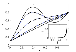
Figure 1: Optimal trajectory in the 1d SSEP for a given final state $\rho_{f}$. Solid lines are $\bar{\rho},\rho_{f}$ and the exact $\rho\left(x,t\right)$ at $t=-0.01,-0.05,-0.2$. Numerical results are shown as dots. Inset: the contribution to the action up to intermediate times.

We now show that the dynamics of the large deviations of slowly varying configurations can be captured by a small number of variables, which describe the long wave-length behavior. This provides an effective large-scale description of $\phi$ in terms of a small number of degrees of freedom. To this end we define a family of functions $\left\{\rho_{i}\left(\mathbf{x}\right)\right\}$ which span the function space, ordered such that $\rho_{1}\left(\mathbf{x}\right)$ is the slowest varying in space, followed by $\rho_{2}\left(\mathbf{x}\right)$, etc.. We then consider an approximation in which the configurations leading to $\rho_{f}$ are restricted to be linear combinations of a finite number of the slowest-varying $\rho_{i}$,

$$\rho_{M}\left(x,t\right)=\bar{\rho}\left(x\right)+\sum_{i=1}^{M}a_{i}\left(t\right)\rho_{i}\left(x\right)\ .$$ (8)

For $M\rightarrow\infty$ this recovers the exact extremal solutions. For finite $M$, when $\rho_{f}$ is itself of the form of Eq. (8) the solutions give upper bounds for the exact value of $\phi\left[\rho_{f}\right]$, since the minimization is only on a subset all histories $\rho\left(x,t\right)$. Below we are interested in how well they approximate the exact solutions.

A natural choice of the functions $\left\{\rho_{i}\left(x\right)\right\}$ are the normal modes of the linearized Hamilton evolution, Eqs. (6) and (7), linearized around $\rho=\bar{\rho}$ and $\hat{\rho}=0$ other_modes . These are obtained by substituting $\rho\left(x,t\right)=\bar{\rho}\left(x\right)+\sum_{i}\rho_{i}\left(x\right)e^{\lambda_{i}t}$, $\hat{\rho}\left(x,t\right)=\sum_{i}\hat{\rho}_{i}\left(x\right)e^{\lambda_{i}t}$ and keeping only linear terms in $\rho_{i}\left(x\right)$ and $\hat{\rho}_{i}\left(x\right)$

$$\lambda_{i}\rho_{i} =\mathbf{\nabla}\cdot\left(D\left(\bar{\rho}\right)\mathbf{\nabla}\rho_{i}\right)-\mathbf{\nabla}\cdot\left(\sigma\left(\bar{\rho}\right)\mathbf{\nabla}\hat{\rho}_{i}\right)\ ,$$ (9a)

$$\lambda_{i}\hat{\rho}_{i} =-D\left(\bar{\rho}\right)\nabla^{2}\hat{\rho}_{i}\ ,$$ (9b)

with boundary conditions $$\rho_{i}=0=\hat{\rho}_{i} \rho\left(x,t\right) \rho \bar{\rho} \hat{\rho}_{i} t\rightarrow-\infty \rho_{f}=\bar{\rho} \hat{\rho}_{i} \rho_{i} \lambda_{i},\hat{\rho}_{i} \rho_{i}\left(x\right) \rho_{i} \int\rho_{i}^{2}dx=1 x=0$$. The solution of these equations is the optimal trajectory of Eq. (4) for small fluctuations of around . These equations admit two types of solutions. In one type, vanish identically. These solutions correspond to the zero-noise evolution, and do not satisfy the initial condition at (except in the trivial case ). The other set of solutions is obtained by first solving Eq. (9b), which is an eigenvalue problem for , independently of . The resulting are then substituted into Eq. (9a), and is solved for. As a convention, we take all functions to be normalized with , and in 1d have a positive slope at .

As a first example we return to the profile $\rho_{f}$ given in Fig. 1, which is of the form $\rho_{f}=\bar{\rho}+\alpha_{1}\rho_{1}+\alpha_{2}\rho_{2}$, where $\lambda_{1,2}$ are the two lowest eigenvalues, $\lambda_{i}=\left(\pi i\right)^{2}$, and $\alpha_{1}=-0.256$, $\alpha_{2}=-0.214$. The modes $\rho_{i}$, for $i=1,2,3$ are shown in Fig. 2(a). We now minimize the action with histories constrained to be of the form of Eq. (8), with $M=2,3,..$. Fig. 2(b) shows the histories for $M=2$ (dashed lines). Even for $M=2$, the large deviation is obtained to within 2%, see Fig. 2(c), suggesting that even at this level the system’s behavior can be captured by an effective model with only two degrees of freedom. Such a small error is striking considering the highly non-linear nature of the problem (as $\rho_{f}$ is far from $\bar{\rho}$), which is generically expected to mix higher modes in significant amounts. By comparison, a local equilibrium approximation (where a space-dependent chemical potential is set to reproduce $\bar{\rho}$) gives a relative error of 16%, whereas extending the linearized dynamics to the full evolution SSEP_spohn gives an error in the large deviation of 67% (mostly due to the long-range Gaussian corrections). This highlights both the importance of non-linearities in this problem, and the success of the truncated approximation.

The mode approximation can also be used as a high precision numerical method. As shown in Fig. 2(c), for $M=15$, the relative error is reduced to $\sim 10^{-5}$, well below the error obtained by a straightforward discretization of space. Indeed similar approaches have been used as numerical tools to improve accuracy in MAM_fin_dim .

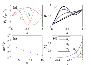
Figure 2: (a) The modes $\rho_{1},\rho_{2},\rho_{3}$. (b) The exact evolution (solid lines) and the evolution with $M=2$ (dashed lines). (c) The relative error $\left(\phi_{M}\left[\rho_{f}\right]-\phi\left[\rho_{f}\right]\right)/\phi\left[\rho_{f}\right]$ for different numbers of modes $M$. (d) The time evolution of $a_{i}$ for $i=1..9$. Modes $a_{5}$ and above cannot be seen on this scale.

The low mode approximation is also useful in cases where an exact analytical solution does not exist. For example, our method allows us to study two-dimensional (2d) systems. In 2d analytic solutions are only known for a set of models which exhibit no long-range correlations. We used one such model, with $D=1$ and $\sigma\left(\rho\right)=2\rho$, corresponding to a model of non-interacting particles, as a benchmark for our method, and found agreement between the numerics and the exact solution (see the Appendix). In what follows we present results for an interacting system, the SSEP in 2d, for which an exact expression for the large deviation is not known. This exhibits the real power of the numerics. To show the generality of the low mode approximation, we take a somewhat arbitrary choice of boundary conditions, $\rho\left(x,y\right)=0.25\sin(3\operatorname{atan}\left(y/x\right))+0.55+0.5y$, on the square domain $A=\left[-1/2,1/2\right]^{2}$, see Fig. 3. The most probable density profile $\bar{\rho}$ is shown in Fig. 3(a), and we present results for the profile $\rho_{f}$ shown in Fig. 3(b), which, as in the 1d discussion, is of the form $\rho_{f}=\bar{\rho}+\alpha_{1}\rho_{1}+\alpha_{2}\rho_{2}$, where $\rho_{1},\rho_{2}$ are the lowest modes in this system, and $\alpha_{1}=0.097,\alpha_{2}=0.128$. Similar results were obtained for other profiles. Fig. 3(c) shows the growth of the modes for $M=2..10$. The first two modes give the exact large deviation to within $2\cdot 10^{-3}$, as estimated by $\left(\phi_{2}\left[\rho_{f}\right]-\phi_{14}\left[\rho_{f}\right]\right)/\phi_{14}\left[\rho_{f}\right]$, see Fig. 3(d). Once more, as in 1d, this means that the evolution is well described by a two-parameter space $\left(a_{1}\left(t\right),a_{2}\left(t\right)\right)$, despite the non-linear nature of the problem. Interestingly, a local equilibrium approximation gives a relatively low error of 1.2%.

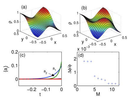
Figure 3: (a) $\bar{\rho}$ and (b) $\rho_{f}$ for a 2d SSEP example. (c) The modes evolution. Solid lines: Amplitudes $a_{i}$ for $i=1..10$. $a_{3}$ and above are hard to distinguish in the scale of the graph. Dashed lines (almost indistinguishable): 2 modes. (d) The relative error $\left(\phi_{M}\left[\rho_{f}\right]-\phi\left[\rho_{f}\right]\right)/\phi\left[\rho_{f}\right]$.

We have shown so far that the large deviation function is well-approximated using only a few modes, provided that $\rho_{f}$ itself is a slowly-varying function of space. Here we discuss how to extend these results to cases where $\rho_{f}$ is not necessarily slowly varying, but has some high-mode content. Recalling that the bulk behavior is governed by equilibrium dynamics, one might expect that small, high-mode perturbations around the low mode behavior would be captured by a local equilibrium theory. In particular, define a local free-energy density $f_{eq,\bar{\rho}}\left(\rho\right)\equiv\int_{\bar{\rho}}^{\rho}d\rho^{\prime}\int_{\bar{\rho}}^{\rho^{\prime}}\frac{2D\left(\rho^{\prime\prime}\right)}{\sigma\left(\rho^{\prime\prime}\right)}d\rho^{\prime\prime}$. In equilibrium, when all boundary densities are equal, this is precisely the free-energy density. We then expect

$$\phi\left[\rho_{f}\right]-\phi\left[\rho_{f,M}\right]\simeq\int\left[f_{eq,\bar{\rho}}\left(\rho_{f}\right)-f_{eq,\bar{\rho}}\left(\rho_{f,M}\right)\right]dx\ ,$$ (10)

where $\rho_{f,M}$ is $\rho_{f}$ projected to the subspace spanned by $\left\{\bar{\rho},\rho_{1},..,\rho_{M}\right\}$. In other words, the error due to truncation of the high modes is approximately accounted for by a local equilibrium theory. We now show that this is indeed the case in an example on the Kipnis–Marchioro–Presutti (KMP) model for heat transfer KMP , whose continuum limit KMP_large_dev gives $D=1$ and $\sigma\left(\rho\right)=2\rho^{2}$ (similar results are obtained for other models). In Fig. 4, we take $\rho_{f}$ of the form $\bar{\rho}+0.463\rho_{1}+0.507\rho_{2}-0.1\left(\rho_{5}+\rho_{6}+\rho_{7}\right)$. For this profile, the LHS of Eq. (10) for $M=2$ equals -0.03667 and the RHS equals -0.03623. Thus Eq. (10) is satisfied with relative accuracy of 1.2%. Hence, for profiles with high mode content the effective low mode description can be corrected for using Eq. (10).

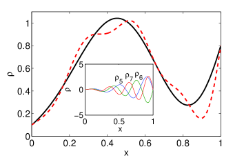
Figure 4: A profile containing only the two lowest KMP modes (solid), and one contaning modes up to 7 modes (dashed). Inset: plot of KMP modes 5,6 and 7.

In summary, our findings suggest that the evolution leading to a “smooth” rare event is smooth: the continuous diffusion $\partial_{t}\rho=\mathbf{\nabla}\cdot\left(D\left(\rho\right)\mathbf{\nabla}\rho\right)+\left\langle small\ noise\right\rangle$, makes an enduring high frequency perturbation highly unlikely. Indeed we show that even when the evolution leading to the rare event is restricted to profiles involving just a few modes, good quantitative agreement with the exact large deviation may be found. This means that the large deviation is well-described in a space involving just a few variables.

Finally, we note that in general the action may have more than a single local minimum, an effect which is well-known in finite-dimensional systems Noise_non_lin_book ; analog_exp ; Maier_Stein ; Graham_Tel ; Dykman . While this does not happen in the well-known models used above in our comparisons, it does in fact exist in other models, and can be studied using the numerical method described here by considering various different final-state trajectories. For example, when two solutions are present, different choices of final-state trajectories will lead to the different local minima local_min_footnote . A detailed account of this issue and its physical implications is beyond the scope of the present work, and will be disscussed elsewhere ours .

I Appendix

I.1 Action evaluation

The action evaluation, including the Lagrange multipliers, is implemented directly in the discrete setting, which gives discrete variants of Eq. (6), along with the boundary conditions. In the numerical implementation, time and space are discretized, and $\rho$ is kept at points $\rho_{i,k}=\rho\left(x_{i},t_{k}\right)$ in 1d, and $\rho_{i,j,k}=\rho\left(x_{i},y_{j},t_{k}\right)$ in 2d. We start by describing the method in 2d, and then discuss the simplifications which occur in 1d.

The action, Eq. (4), is discretized as $S=\sum_{k}\Delta S_{k}$ where $\Delta S_{k}$ is the value of $S$ associated with the time interval $\left[t_{k},t_{k+1}\right]$. This allows for the time resolution to vary. For each $k$ separately, $\Delta S_{k}$ is evaluated as

$$\Delta S_{k}=\Delta t\sum_{i,j}\left(S_{i+1/2,j}^{x}+S_{i,j+1/2}^{y}\right)\ ,$$ (11)

where $\Delta t=t_{k+1}-t_{k}$. $S_{i+1/2,j}^{x}$ corresponds to the bond connecting $\left(i,j\right)$ to $\left(i+1,j\right)$ (and similarly for other half-integer indices).

Let $\rho_{i,j}\equiv\frac{1}{2}\left(\rho_{i,j,k+1}+\rho_{i,j,k}\right)$. Then $S_{i+1/2,j}^{x}$ is given by

$$S_{i+1/2,j}^{x}=\frac{\left(J_{i+1/2,j}^{x}+D\left(\rho_{i+1/2,j}\right)\left(\partial_{x}\rho\right)_{i+1/2,j}\right)^{2}}{2\sigma\left(\rho_{i+1/2,j}\right)}$$ (12)

with $\rho_{i+1/2,j}\equiv\frac{1}{2}\left(\rho_{i,j}+\rho_{i+1,j}\right)$, $\left(\partial_{x}\rho\right)_{i+1/2,j}\equiv\left(\rho_{i+1,j}-\rho_{i,j}\right)/\Delta x$, and a similar expression for $S_{i,j+1/2}^{y}$. The currents $J^{x},J^{y}$ are constrained to satisfy a discretized version of the continuity equation, Eq. (1),

$$0 =R_{ij}\equiv\left(\partial_{t}\rho\right)_{i,j}$$

$$+\frac{J_{i+1/2,j}^{x}-J_{i-1/2,j}^{x}}{\Delta x}+\frac{J_{i,j+1/2}^{y}-J_{i,j-1/2}^{y}}{\Delta y}\ ,$$ (13)

where $\left(\partial_{t}\rho\right)_{i,j}\equiv\left(\rho_{i,j,k+1}-\rho_{i,j,k}\right)/\Delta t$, and $\Delta x,\Delta y$ are the (constant) spacings in the $x$- and $y$-directions. To minimize the currents subject to Eq. (13), we define $\Delta G_{k}=\Delta S_{k}-\sum_{ij}\hat{\rho}_{ij}R_{ij}$. Differentiating $\Delta G_{k}$ with respect to the currents gives

$$J_{i+1/2,j}^{x} =-D\left(\rho_{i+1/2,j}\right)\left(\partial_{x}\rho\right)_{i+1/2,j}$$ (14)

$$+\sigma\left(\rho_{i+1/2,j}\right)\frac{\hat{\rho}_{i+1,j}-\hat{\rho}_{i,j}}{\Delta x}$$

with a similar expression for $J_{i,j+1/2}^{y}$. This is a discrete variant of $\mathbf{J}=$ $-D\left(\rho\right)\mathbf{\nabla}\rho+\sigma\left(\rho\right)\mathbf{\nabla}\hat{\rho}$. Substituting Eq. (14) into Eq. (13), one obtains a linear set of equations for the $\hat{\rho}$-variables, which corresponds to Eq. (6). These are solved to find the $\hat{\rho}$-variables. Note that on boundary sites Eq. (13) involves only three currents (or two at corners of the lattice), which is equivalent to setting $\hat{\rho}_{i,j}=0$ for $i,j$ outside the lattice. This corresponds to the boundary conditions $\left.\hat{\rho}\left(x,t\right)\right|_{x\in\partial A}=0$ in the continuum.

Given the $\hat{\rho}$ values, the final expression for $S$ is obtained by combining Eqs. (11),(12) and (14), and reads

$$\Delta S_{k}=\frac{1}{2}\Delta t\Delta x\Delta y\sum_{i,j}\left[\begin{array}[c]{c}\sigma\left(\rho_{i+1/2,j}\right)\left(\frac{\hat{\rho}_{i+1,j}-\hat{\rho}_{i,j}}{\Delta x}\right)^{2}\\ +\sigma\left(\rho_{i,j+1/2}\right)\left(\frac{\hat{\rho}_{i,j+1}-\hat{\rho}_{i,j}}{\Delta y}\right)^{2}\end{array}\right]\ ,$$ (15)

which serves as the discrete analog of $\tilde{S}\left[\rho\right]=\frac{1}{2}\int dtd\mathbf{x}\sigma\left(\rho\right)\left(\mathbf{\nabla}\hat{\rho}\right)^{2}$. This concludes the evaluation of the action $S$ for a given $\rho$. This procedure is used as a building block in the optimization algorithm, where $S$ is evaluated for different histories $\rho\left(x,t\right)$, see the main text.

In 1d the above scheme is somewhat simplified. Of course, only terms in the $x$ direction appear. The continuity Eq. (13) is now $J_{i+1/2}^{x}=J_{i-1/2}^{x}-\Delta x\left(\partial_{t}\rho\right)_{i}$, so $J_{i+1/2}^{x}=J_{c}-\Delta x\sum_{n=1}^{i}\,\left(\partial_{t}\rho\right)_{n}$, where $J_{c}$ is independent of the position $i$ (but may depend on time). Summing over Eq. (14), and using $\hat{\rho}_{0}=0$ we find

$$\hat{\rho}_{i}=\Delta x\sum_{m=0}^{i-1}\frac{D\left(\rho_{m+1/2}\right)\left(\partial_{x}\rho\right)_{m+1/2}+J_{c}-\Delta x\sum_{n=1}^{m}\,\left(\partial_{t}\rho\right)_{n}}{\sigma\left(\rho_{m+1/2}\right)}\ ,$$ (16)

where $J_{c}$ is fixed by requiring that the boundary condition $\hat{\rho}_{N_{x}+1}=0$ holds.

As an additional tool to improve accuracy, it is possible to interpolate $\rho\left(x,t\right)$ onto a finer grid in $\left(x,t\right)$ before evaluating the action. This simple step improves accuracy and stability at low resolutions. In the example presented below, we use this technique to double the time resolution.

Computations involving modes use exactly the same action evaluation scheme, and only differ in the profiles $\rho\left(x,t\right)$ allowed in the density optimization process.

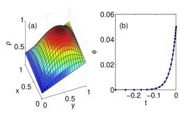
Figure 5: Comparison of numerical results with a 2d non-interacting model. (a) The profile tested. (b) The exact evolution of the large deviation (solid line) compared with the numerics (points).

I.2 Benchmark for 2d numerical method

The algorithm was tested in 2d against the model $\sigma=2\rho$ and $D=1$. This model is a particular case of the open boundary Zero Range process ZRP ; BertiniPRL , and its large deviation is given by

$$\phi\left[\rho_{f}\right]=\int d^{2}x\left(\rho_{f}\ln\frac{\rho_{f}}{\bar{\rho}}+\bar{\rho}-\rho_{f}\right)\ .$$ (17)

$\phi\left[\rho_{f}\right]$ was calculated for $\rho_{f}$ in Fig. 5(a). Fig. 5(b) shows a comparison of the numerical method with the exact result at a relatively low resolution, with $N_{x}=N_{y}=8$ divisions in each space dimension and $N_{t}=25$ divisions in time, starting from $\tau=-0.3$. The profiles were interpolated onto a grid with twice the time resolution before the action evaluation. The relative error in $\phi\left[\rho_{f}\right]$ was $5\cdot 10^{-4}$.

References

- (1) P. G. Bolhuis, D. Chandler, C. Dellago, P. L. Geissler, Annu. Rev. Phys. Chem. 53, 291-318 (2002)
- (2) A. Kamenev and B. Meerson, Phys. Rev. E. 77, 061107 (2008)
- (3) S. Coleman, Phys. Rev. D 15, 2929–2936 (1977)
- (4) F. Moss and P. V. E. McClintock, ed., Noise in Nonlinear Dynamical Systems, Cambridge University Press, Cambridge (1989)
- (5) D. G. Luchinsky, P. V. E. McClintock, and M. I. Dykman, Rep. Prog. Phys., 61(8):889-997 (1998)
- (6) R. S. Maier and D. L. Stein, Phys. Rev. E, 48(2):931-938 (1993)
- (7) R. Graham and T. Tél, Phys. Rev. Lett. 52, 9–12 (1984)
- (8) M.I. Dykman, M.M. Millonas and V.N. Smelyanskiy, Phys. Lett. A, 195 (1994), 53
- (9) H. Touchette, R. J. Harris, Large deviation approach to nonequilibrium systems, in R. Klages, W. Just, C. Jarzynski (eds), Nonequilibrium Statistical Physics of Small Systems: Fluctuation Relations and Beyond, Wiley-VCH, Weinheim (2012)
- (10) M. I. Freidlinand A. D. Wentzell, Random Perturbations of Dynamical Systems, Springer-Verlag (1984)
- (11) B. Derrida, J. Stat. Mech. P07023 (2007)
- (12) C. Giardinà, J. Kurchan, and L. Peliti, Phys. Rev. Lett. 96, 120603 (2006)
- (13) V. Lecomte and J. Tailleur, J. Stat. Mech. P03004 (2007)
- (14) J. Tailleur and V. Lecomte, AIP Conf. Proc. 1091, 212-219 (2008)
- (15) C. Giardina, J. Kurchan, V. Lecomte, J. Tailleur, J. Stat. Mech. 45 4 (2011)
- (16) D. Passerone and M. Parrinello, Phys. Rev. Lett. 87, 108302 (2001). W. E, W. Ren and E. Vanden-Eijnden, Commun. Pure Appl. Math. 57, 637 (2004). X. Wan, J. Comp. Phys. 230 (2011) 8669–8682. F. Bouchet, J. Laurie and O. Zaboronski, J. Phys. Conf. Ser. 318 (2011) 022041
- (17) Ya. M. Blanter and M. Büttiker, Physics Reports, 336, 1-2 (2000), W. Dieterich, P. Fulde and I. Peschel, Adv. in Phys. 29, 527-605 (1980)
- (18) C. Kipnis, C. Marchioro and E. Presutti, J. Stat. Phys. 27 65 (1982)
- (19) C. Kipnis and C. Landim, Scaling Limits of Interacting Particle Systems (Springer, New York, 1999)
- (20) L. Bertini, A. De Sole, D. Gabrielli, G. Jona-Lasinio, and C. Landim, Phys. Rev. Lett. 87, 040601 (2001)
- (21) L. Bertini, A. De Sole, D. Gabrielli, G. Jona-Lasinio, and C. Landim, J. Stat. Phys. 107, P07014 (2002)
- (22) A. N. Jordan, E. V. Sukhorukov and S. Pilgram, J. Math. Phys. 45 4386-4417 (2004)
- (23) J. Tailleur, J. Kurchan and V. Lecomte, J. Phys. A: Math. Theor. 41 505001 (2008)
- (24) P. I. Hurtado and P. L. Garrido, Phys. Rev. Lett. 107, 180601 (2011)
- (25) P. I. Hurtado et. al., Proc. Natl. Acad. Sci. USA. 108(19) 7704–7709 (2011)
- (26) V. Elgart and A. Kamenev, Phys. Rev. E 70, 041106 (2004)
- (27) G. Bunin, Y. Kafri, D. Podolsky, in preparation.
- (28) Every history which locally minimizes the action will be found by a final state trajectory which follows this history.
- (29) H. Spohn, J. Phys. A: Math. Gen. 16 4275 (1983)
- (30) B. Derrida, J. L. Lebowitz, and E. R. Speer, J. Stat. Phys. 107 775-810 (2002)
- (31) Other choices of modes, such as simple plane waves were also tested, and also give good results, but with slower convergence.
- (32) L. Bertini, D. Gabrielli and J. Lebowitz, J. Stat. Phys. 121 843 (2005)