All Curled Up: A Numerical Investigation of Shock-Bubble Interactions and the Role of Vortices in Heating Galaxy Clusters

Abstract

Jets from active galactic nuclei in the centers of galaxy clusters inflate cavities of low density relativistic plasma and drive shock and sound waves into the intracluster medium. When these waves overrun previously inflated cavities, they form a differentially rotating vortex through the Richtmyer-Meshkov instability. The dissipation of energy captured in the vortex can contribute to the feedback of energy into the atmospheres of cool core clusters. Using a series of hydrodynamic simulations we investigate the efficiency of this process: we calculate the kinetic energy in the vortex by decomposing the velocity field into its irrotational and solenoidal parts. Compared to the two-dimensional case, the 3-dimensional Richtmyer-Meshkov instability is about a factor of 2 more efficient. The energy in the vortex field for weak shocks is $E_{vortex}\approx\rho_{ICM}\Delta\,v_{shock}^{2}V_{bubble}$ (with dependence on the geometry, density contrast, and shock width). For strong shocks, the vortex becomes dynamically unstable, quickly dissipating its energy via a turbulent cascade. We derive a number of diagnostics for observations and laboratory experiments of shock-bubble interactions, like the shock-vortex standoff distance, which can be used to derive lower limits on the Mach number. The differential rotation of the vortex field leads to viscous dissipation, which is sufficiently efficient to react to cluster cooling and to dissipate the vortex energy within the cooling radius of the cluster for a reasonable range of vortex parameters. For sufficiently large filling factors (of order a few percent or larger), this process could thus contribute significantly to AGN feedback in galaxy clusters.

1. Introduction

While the gaseous atmospheres of galaxy clusters are virialized, they are often far from relaxed. Cooling gas can condense, form stars, and funnel down to the central galaxy to feed the supermassive black hole in its center. Gas can enter the intra-cluster medium (ICM) through accretion from cosmic filaments, ram pressure stripping of galaxies, jets emanating from active galactic nuclei (AGN), and galactic outflows due to supernova explosions.

The ICM has characteristic temperatures $\gtrsim 2$ keV and central densities of order $\lesssim 0.01\,{\rm cm}^{-3}$, implying that the cooling time of the central cluster gas in many clusters is much shorter than the Hubble time.

However, observations with XMM-Newton and the Chandra X-ray telescope (CXO) over the past decade have shown that cooling to temperatures below about 1.5 keV is suppressed. In order for the gas in the ICM to maintain its temperatures over time, energy must be added to counterbalance the radiative energy losses.

Extragalactic jets from AGN can provide this counterbalance due to the very large energies injected into the ICM. McNamara & Nulsen (2007) provide an excellent overview of the current paradigm of AGN feedback.

It is now well established that jet feedback happens through inflation of X-ray cavities (e.g., Churazov et al., 2000; McNamara et al., 2000; Fabian et al., 2000; Blanton et al., 2001; Heinz et al., 2002; Rafferty et al., 2006, and references therein). At a minimum, the jets have to supply enough energy to create the enthalpy associated with the radio bubbles / X-ray cavities they inflate in the ICM by pushing aside the ICM and filling these cavities with synchrotron emitting particles.

The estimates of the enthalpy ($4pV$) from observed cavities suggest that AGN can indeed provide sufficient energy, though much of this energy has a non-thermal form: The bubbles store up to 75% of it as non-thermal internal energy. Depending on the inflation dynamics, an appreciable fraction of the remaining energy can go into sound or shock waves. In order to understand how feedback works as a process, it is important to understand how much of this energy is thermalized, and where.

AGN are among the most highly variable phenomena, and jets in particular are well known for being non-stationary. It has been suggested that observations of multiple generations of cavities and successive concentric shock and sound waves in many clusters are evidence for strong variability on duty-cycle time scales of order 1-10 million years, though dynamic instabilities, buoyancy, and shear within the jets themselves can also account for some of these observations (Morsony et al., 2010; Soker et al., 2009).

A detached cavity/bubble will buoyantly rise through the ICM, moving further away from the central AGN, while the AGN creates a new bubble and an associated outgoing shock wave. While individual clusters only afford us a snapshot view of this process, the multiple generations of bubbles and waves observed in a number of nearby clusters, and the high frequency of bubbles in cool core clusters suggest that this process is constantly ongoing, filling the cluster with a spectrum of bubbles and waves (Begelman, 2001).

An increasing body of observations provides direct evidence of weak shocks and non-linear sound waves in clusters with central radio galaxies (Fabian et al., 2006; Forman et al., 2007; Graham et al., 2008; Blanton et al., 2009; Million et al., 2010). As they propagate outward, these waves must interact with previously inflated bubbles. This interaction and the possible effect it can have on the thermodynamics of the cluster is the subject of this paper.

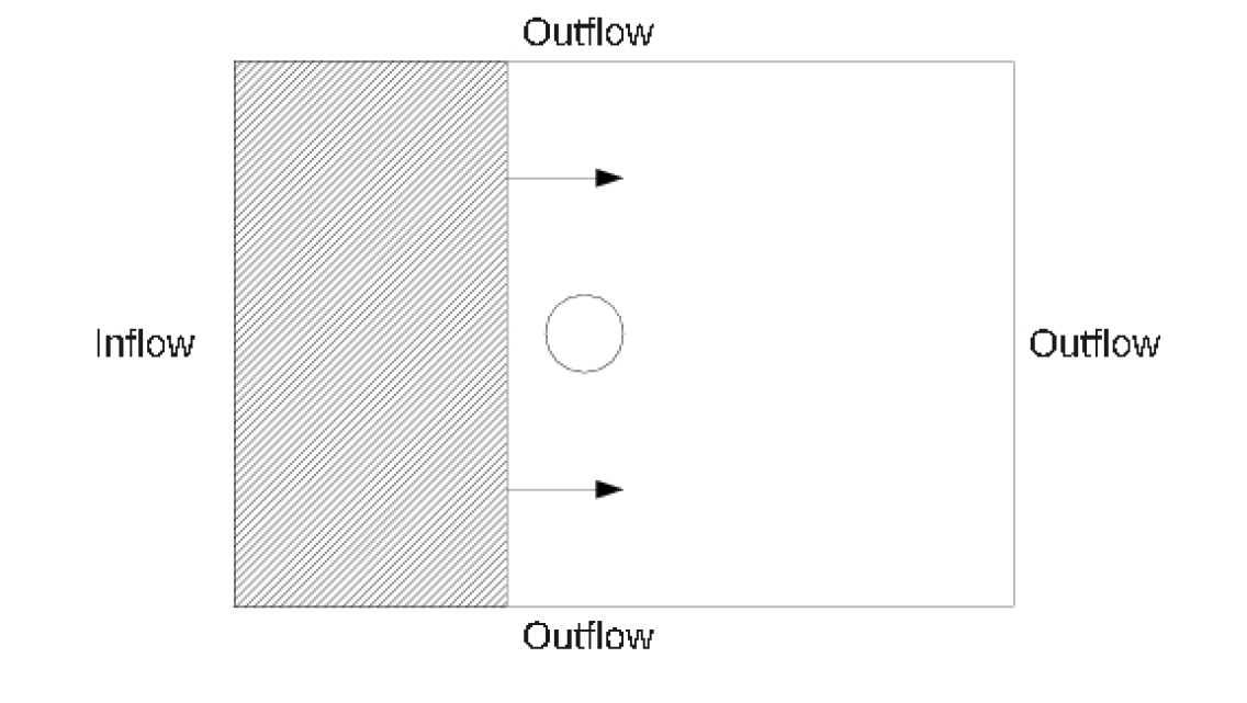
Figure 1.— Boundary Conditions. $x$-axis has mixed inflow/outflow boundary conditions, while the $y$- and $z$-axes have outflow boundary conditions.

Heinz & Churazov (2005) (henceforth abbreviated as HC05) provided a two dimensional study of shock–bubble interactions. While sound waves and weak shocks themselves have low efficiencies for (non-adiabatic) dissipation (sound waves are completely non-dissipative in the absence of viscosity or thermal conduction), HC05 suggested that the dynamics of the interaction of waves with previously inflated bubbles could extract energy from the shock/sound wave and transform it to heat.

This potential heating mechanism for the ICM derives from the Richtmyer-Meshkov Instability (RMI) (Richtmyer, 1960; Meshkov, 1969; Brouillette, 2002) which operates when a shock encounters a curved interface between two fluids. The proposed mechanism could work in concert with other forms of ICM heating by shock waves and bubbles previously proposed in the literature (e.g., McNamara et al., 2005; Mathews et al., 2006).

The interaction of a shock wave with underdense bubbles has been investigated in a broad body of work in the broader fluid dynamical community, both experimentally and theoretically (Picone & Boris, 1988; Quirk & Karni, 1996; Bagabir & Drikakis, 2001; Layes et al., 2005; Giordano & Burtschell, 2006; Ranjan et al., 2007, 2008a, 2008b; Niederhaus et al., 2008; Layes et al., 2009). However, none of these papers discuss the prospect of the ensuing visco-rotational heating, and the extraction of rotational kinetic energy suggested by HC05.

Many previous studies examined the RMI through the use of 2D simulations (e.g. Picone & Boris (1988)). Such a treatment necessarily excludes the impact of any movement of material through the plane of simulation, eliminating some important aspects of vorticity generation, as we will show in this paper.

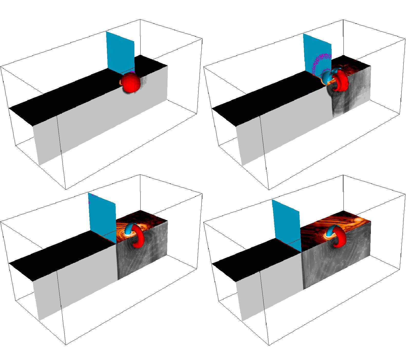
Figure 2.— 3D renderings of the shock–bubble interaction. The short vertical plane that moves across the box is an iso-pressure contour that represents the shock front; the red surface is an iso-density contour that shows the under-dense sphere/vortex ring; the long (light-grey) vertical plane shows a cut through the baroclinic term, $|\nabla p\times\nabla\rho|$, and the long (dark-grey) horizontal plane show a cut through the enstrophy $\rho\omega^{2}$ (a proxy for the energy in the rotational velocity field). Behind the blue-gree pressure contour, we show a magenta iso-density contour. In locations where the two surfaces cross, the density and pressure gradient are mis-aligned, indication locations where vorticity is generated.

Returning to the astrophysical context, other studies have followed the evolution of X-ray cavities / radio bubbles under the influence of buoyancy, using both hydrodynamic and MHD simulation, (Churazov et al., 2001; Gardini & Ricker, 2004; Reynolds et al., 2005; Jones & De Young, 2005; Ruszkowski et al., 2007; Liu et al., 2008; Sternberg & Soker, 2008; Pavlovski et al., 2008; O’Neill et al., 2009; Dong & Stone, 2009).

The effect of shock-bubble interaction in the context of radio relics in the outer cluster was considered by Enßlin & Brüggen (2002). However, outside of Heinz & Churazov (2005), none have investigated the effects of shock traversal of a cavity in the core of a cluster, and the associated transfer of energy into the vortex.

Name	Size [$R_{\rm bub}$]	Properties
Varying density	16x8x8	Density Ratios $\rho_{\text{ICM}}/\rho_{\text{bub}}$ of 50, 20, 10, 5, & 2
Varying Mach Numbers	64x8x8	Mach 1.02, 1.07, 1.25, 1.5, 1.75, 2*, 4*, & 8*
Varying Mach (2.5D)	128x8	Mach 2, 4, & 8
Multiple Bubbles	64x16x16	Impact Parameter of $0,1,2,3,4\;R_{\text{bub}}$
Multiple Bubbles	64x8x8	3 Families of 2, 4, & 8 bubbles
Top-hat widths	16x8x8	Widths of $\lambda=0.5,0.6,1,1.2,2\;R_{\text{bub}}$

Table 1List of simulation parameters. All simulations, except for the starred ones, have a maximum effective refinement of 5 levels (corresponding to a resolution of 32 cells across a bubble diameter). The starred simulations, Mach 2, 4, and 8, have a maximum refinements of 7, 6, and 7, respectively. Simulations indicated as 2.5D are axi-symmetric. Box sizes are given in units of bubble radii (the simulations are scale free).

The observational appearance of shock-generated vortices in clusters was described in a companion paper (Heinz et al., 2011), showing that, while the interaction of waves and cavities in clusters is unavoidable, a direct detection with X-ray methods will be difficult (the so-called “radio ear” in the Virgo cluster might be the best example of a vortex ring, given that it is trailing relatively closely behind a moderate Mach number shock - see Owen et al. 2000; Heinz et al. 2011).

In this paper, we extend the study of HC05 to 3D, derive conditions under which the RMI can effectively dissipate wave energy and heat a cluster on a time scale shorter than the cooling time, and compare our results to the general body of work on the RMI beyond the context of clusters, both in the laboratory and in theory and simulation. We ignore conduction, viscosity, gravity, and magnetic fields in the simulations themselves, but we extend our discussion to an estimate of the viscous dissipation rate of cluster-scale vortices. We also limit ourselves to the case of underdense bubbles. For a study of the inverse density scenario of shock-cloud interactions, we refer the reader to, for example, Klein et al. (1994).

In §2, we describe the methods used for our setup and analysis. Section 3 discusses our results, §4 discusses dissipation in the ICM, and §5 presents our conclusions.

2. Methods

We performed a large set of 3D simulations, spanning a range in important simulation parameters. Before describing the results in general, we will first describe our simulation setup in §2.1 and our analysis methods in §2.2. For reference, our fiducial simulation is a Mach 2 shock running over an underdense bubble. We will use this simulation as a baseline to compare to other cases and to make the connection to HC05.

We present a description and list of our entire set of simulations and describe in §2.4, followed by a discussion of the results.

2.1. Simulation setup

We use the publicly available hydro code FLASH 3.3 (Fryxell et al., 2000; Dubey et al., 2008) which solves the hydrodynamic equations on an adaptive Eulerian grid (in our case, without gravity):

$$\frac{\partial\rho}{\partial t}+\nabla\cdot\left(\rho\mathbf{v}\right) = 0$$ (1)

$$\frac{\partial\rho\mathbf{v}}{\partial t}+\nabla\cdot\left(\rho\mathbf{v}\mathbf{v}\right)+\nabla P = 0$$ (2)

$$\frac{\partial\left(\epsilon+\rho\left|\mathbf{v}\right|^{2}/2\right)}{\partial t}+\ \ \ \$$

$$\nabla\cdot\left[\left(\epsilon+\rho\left|\mathbf{v}\right|^{2}/2+P\right)\mathbf{v}\right] = 0$$ (3)

for the fluid density $\rho$, pressure $P$, velocity $\mathbf{v}$, and internal energy density $\epsilon$.

FLASH employs the piece-wise parabolic method (PPM) to solve the Riemann problem to second order (Colella & Woodward, 1984; Woodward & Colella, 1984). PPM uses a shock capturing scheme to treat shocks.

We include a tracer fluid inside the bubble so that we can easily track material initially inside the bubble as the simulation evolves. Throughout the simulations presented in this paper, we use an adiabatic equation of state, $P=\left(\gamma-1\right)\epsilon$ with ratio of specific heats of $\gamma=5/3$.

The numerical setup used in this paper is similar to that described in HC05: An underdense bubble (typically with density contrast 100 unless otherwise indicated) is introduced to be at rest in, and in pressure equilibrium with a uniform, stationary background medium.

We introduce a shock of Mach number $M$ traveling along the x-direction downstream of the bubble such that it will overrun the bubble in the course of the simulation. The shock satisfies the Rankine-Hugoniot jump conditions and sets the inflow boundary conditions on the upstream x-axis to continually inject shocked gas into the computational box, following the classic semi-infinite shock-tube prescription. We use outflow boundary conditions for the remaining faces of the grid (see the sketch of the simulation setup in Fig 1).

We set the size of of the $y$- and $z$-axes equal to $8R_{\text{bub}}$ and we vary the length of the $x$-axis to ensure the relevant dynamics of the bubble are captured within the simulation box, with a minimum value of $8R_{\text{bub}}$. Unless otherwise noted, we used a maximum refinement level of 5, corresponding to a resolution of 32 grid points across the bubble diameter and an effective grid size of $(256+)\times 128\times 128$. We used density as our refinement variable in order to refine both on the shock front and the bubble.

For translation into physical units, a gas density of $n=0.01\,{\rm cm^{-3}}$, a bubble radius of $R=10\,{\rm kpc}$, and a gas temperature of $T=5keV$ give typical box sizes of $80\,{\rm kpc}$ on a side and lengths from $240\,{\rm kpc}$ upward and characteristic time (the sound crossing time of the bubble) of $1.8\times 10^{7}\,{\rm yrs}$.

In this investigation, we vary the shock Mach number, the shape of the bubble (we consider spherical and cylindrical bubble), the density contrast, and the number of bubbles, and also investigate the effect of changing the width of the shock (from semi-infinite to finite).

Because we were aiming to extend the 2D study from HC05 to three dimensions, and because we are aiming to study a very basic hydrodynamic scenario using a new analysis tool (Helmholtz decomposition of the velocity field), we specifically kept the numerical setup very simply, as described above: We did not include gravity in the simulations, as we wished to investigate the efficiency of the RMI, not of the buoyancy instability. We also excluded magnetic fields from this particular investigation, and we kept the simulations as inviscid as possible, given the level of numerical viscosity at the resolution allowed by our computational limitations, i.e., we did not include a prescription for fluid viscosity in the code.

Most of the simulations were run in-house on a 72 node Beowulf cluster, typically using 64 cores and 128 GBytes of ram. We estimate a total runtime of 150,000 CPU hours, including analysis.

Name	Size [$R_{\rm cyl}$]	Properties
Varying Mach Numbers	Varied	Mach 1.02, 1.07, 1.25, 1.5, 1.75, 2, 4, & 8
Varying Angles	32x16x16	$L=4\;R_{\text{bub}}$, Angles = 0, 30, 60, 90 degrees
Varying Lengths	256x(16/32)2	$x$-axis: $1,2,4,8\;R_{\text{bub}}$
Varying Lengths	256x16x16	$y$-axis: $1,2,4,8\;R_{\text{bub}}$

Table 2List of simulation parameters for shock-cylinder interactions. All simulations have a maximum effective refinement of 5 levels. sizes are measured in cylinder radii. For the various Mach numbers, some simulations have shorter sides parallel to the cylinder axis and use periodic boundary conditions. Simulations of cylinders with axes parallel to the $x$-axis (i.e., the shock normal), the box size in the $y$ and $z$ directions is set to 32 cylinder radii to ensure we contained all of the relevant dynamics within our simulation volume.

2.2. Velocity decomposition

Throughout this paper we will analyze simulations with the aim of characterizing the energy extracted from the passing shock wave and deposited in the vortex, following HC05.

We use Helmholtz’s theorem to split up a 3D velocity field into two components: an irrotational part and a rotational (solenoidal) part. We can thus write the velocity field as:

$$\mathbf{v} =\mathbf{v}_{I}+\mathbf{v}_{R} \nabla\times\mathbf{v}_{I} =0 \nabla\cdot\mathbf{v}_{R} =0$$ (4)

In essence, this method of extracting the rotational velocity and, consequently, the rotational kinetic energy (RKE), is equivalent to divergence cleaning of the 3D velocity field (Balsara, 1998).

While we use discrete Fourier transforms for this decomposition (which is strictly only applicable in the case of periodic boundary conditions), we show in a separate paper (Friedman & Heinz, In Prep.) that this technique provides an excellent approximation of the rotational velocity field in cases where the vorticity, $\omega\equiv\nabla\times\mathbf{v}$ vanishes near the edges of the simulation. To ensure that we satisfy this condition we use a sufficiently large grid around the bubble/vortex.

2.3. Rotational kinetic energy

Following HC05, it is straight forward to estimate the scale on which the RMI can extract energy from the passing wave. For a bubble overrun by a shock with velocity jump $\Delta v=v_{1}-v_{2}$, we can express the kinetic energy density of the density perturbation, seen from the downstream/shocked frame, as $e_{\rm kin}=(\rho_{1}-\rho_{\rm bubble})\Delta v^{2}/2\sim\rho_{1}\Delta v^{2}/2$. For a bubble with an initial volume of $V_{\rm bubble}$, the fiducial energy scale of the problem is therefore simply

$$E_{\rm fid}=e_{\rm kin}V_{\rm bubble}=\rho_{1}\frac{\Delta v^{2}}{2}V_{\rm bubble}$$ (5)

After measuring the actual extracted kinetic energy $E_{\rm rot}$ in the vortex in the downstream frame as

$$E_{\rm rot}=\int dV\,\rho\frac{v_{\rm rot}^{2}}{2}$$ (6)

from our simulation, we can define an efficiency factor, $g_{2}$, as

$$g_{2}\equiv\frac{E_{\text{rot}}}{E_{\text{fid}}}=\frac{E_{\text{rot}}}{\frac{1}{2}V_{\text{bubble}}\rho_{1}\Delta v^{2}}$$ (7)

Given the shift to the rest frame to the upstream/unshocked material, we have:

$$\Delta v \equiv v_{1}-v_{2}=c_{s}M\left[\frac{\frac{2}{M^{2}}+\left(\gamma-1\right)}{\gamma+1}-1\right]$$ (8)

We can derive an alternative representation for $g$ by expressing the energy density of the approaching shocked gas in the upstream material,

$$g_{1} \equiv\frac{E_{\text{rot}}}{\frac{1}{2}V_{\text{bubble}}\rho_{2}{\Delta v}^{2}}$$ (9)

$$=g_{2}\frac{\left(\gamma+1\right)+\left(\gamma-1\right)\left(M^{2}-1\right)}{\left(\gamma+1\right)M^{2}}<g_{2}$$

$g_{1}$ is associated with $\rho_{2}$, the downstream/shocked density, and $g_{2}$ is associated with $\rho_{1}$, the upstream/unshocked density. In other words, $g_{2}$ measures the bubble energy from the point of view of the shocked, downstream/shocked medium, compared to the kinetic energy missing from the evacuated bubble volume approaching the shock. $g_{1}$ represents the ratio of the rotational kinetic energy to the kinetic energy in the downstream/shocked volume contained within the bubble volume (i.e., from the point of view of the upstream/unshocked , unshocked medium). We will use $g_{1}$ throughout the rest of the paper unless otherwise noted, with easy conversion given eq. (9).

2.3.1 Vorticity Evolution

To illuminate the development of the RMI, it is instructive to consider the vorticity equation (the curl of the Euler equation):

$$\frac{D\mathbf{\omega}}{Dt} =\underbrace{(\mathbf{\omega}\cdot\mathbf{\nabla})\mathbf{v}}_{\text{Vortex Stretching}}-\underbrace{\mathbf{\omega}(\mathbf{\nabla}\cdot\mathbf{v})}_{\text{Vortex Compression}}$$ (10)

$$\quad+\underbrace{\frac{1}{\rho^{2}}(\nabla\rho\times\nabla p)}_{\text{Baroclinic}}$$

The last term in 10 is commonly referred to as the baroclinic term, and it is present in both 2D and 3D. While the vortex compression term is present in both 2D and 3D simulations, the vortex stretching term is present only in the 3D case. It represents $m\geq 1$ modes, since for the $m=0$ mode the $\phi$-derivatives vanish (this is the axi-symmetric 2.5D case described in §2.4).

2.4. Simulation table

Using our fiducial run as a baseline, we modified the simulations by changing the number of bubbles, the Mach number, the width of shocked material ($\lambda$), the bubble density, and the bubble geometry relative to the shock front. The grid of simulations discussed in the following is laid out in tables 1 and 2.

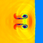
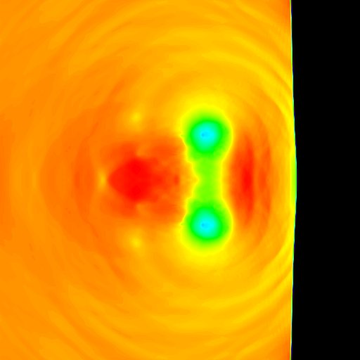
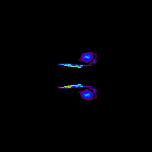
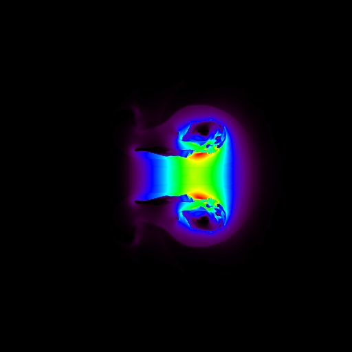
Figure 3.— 2D slices through the center of the simulations box show density (top left), pressure (top right), tracer fluid mass fraction (bottom left), and rotational kinetic energy (bottom right) for a Mach 2 shock, spherical bubble, simulated in a uniform grid ($1024\times 512\times 512$) grid. The acoustic velocity field is visible as roughly spherical outgoing waves, while the primary and secondary vortex rings (PVR and SVR, respectively) are visible as dark, low-density enclosures in the density.

In simulations with cylindrical bubbles instead of spheres, we label cylinders with axes perpendicular to the shock normal “infinite” cylinders because they represent a 3D extension of the plane-parallel 2D circular bubble in HC05. The main families of simulations investigate the dependence of $g$ on fundamental parameters of the hydrodynamics: Mach number, density ratio of bubble to environment, and shock thickness.

Due to the strong long–term time dependence we find in the case of high Mach number shocks (see Fig. 9) that was absent in the 2D simulations of HC05, we decided to investigate a 2.5 dimensional (axi-symmetric) analog of the three dimensional spherical bubble case. Using cylindrical coordinates, $(r,z)$, and placing the center of the bubble at $r=0$, we reproduced the set of simulations of spherical bubbles for different Mach numbers. To calculate the RKE we then mapped the 2.5D cylindrical velocities onto a 3D Cartesian grid and treated them the same way as we treat our 3D regular simulations.

Throughout most of our simulations we use a shock driven by a semi-infinite piston, i.e., a shock with thickness $\lambda\gg R_{\text{bub}}$. As shown in HC05, the efficiency of the RMI depends on $\lambda$ when $\lambda\sim R$. Extending this test to 3D, we simulate shocks with finite width. The resulting shock has a top-hat structure at $t=0$. At later times, the back end of the shock expands into a rarefaction wave.

2.5. Description of bulk dynamical properties

The general evolution of a bubble subject to the RMI has been described in numerous publications. In the context of clusters, we refer the reader to HC05 and (Enßlin & Brüggen, 2002). We will only briefly review the evolution, illustrating a few noteworthy points using rendered images from our simulations.

2.5.1 Fiducial Run

Fig. 2 shows the interaction of a single spherical bubble with a Mach 2 shock, our fiducial case. As expected, the shock enters the bubble and the pressure increase quickly and traverses the bubble, in effect “smearing out” the shock across the entire bubble surface. At the same time, the bubble has negligible inertial density, implying that the shocked material travels quickly through the bubble, which leads to the formation of a vortex ring such that $\hat{\vec{r}}\cdot\left(\vec{\omega}\times\hat{\vec{n}}\right)>0$, where $\hat{\vec{r}}$ is the vector from the vortex axis to the vortex ring, $\vec{\omega}$ is the vorticity inside the vortex, and $\hat{\vec{n}}$ is the shock normal, aligned with the shock velocity. Figure 2 shows the primary vortex ring as a red density contour surface.

The figure also shows the magnitude of the baroclinic term and the local enstrophy, $\rho\omega^{2}$ (related to the rotational kinetic energy). The interaction generates vorticity whenever the baroclinic term in equation 10 does not vanish.

Figure 3 shows 2D slices through some of the relevant fluid variables in our fiducial Mach 2 run.

2.5.2 Non-Linear Vortex Interaction: Simulations of Multiple Bubbles

While the simulation of a single spherical bubble presents the cleanest possible numerical laboratory to study the efficiency of the RMI, one of the questions we aimed to investigate is whether and how $g_{1}$ depends on complications like non-sphericity of the bubble and non-linear interaction of vortex rings from multiple neighboring bubbles.

We designed two sets of numerical experiments to investigate the interaction of multiple vortex rings and its effect on $g_{1}$. To facilitate comparison with other simulation series and with the fiducial run, we simulated a Mach 2 shock.

The first approach places two bubbles offset from each other by $4\;R_{\text{bub}}$ in the $x$ direction (the shock-propagation direction) and displaced in the $y$ direction (perpendicular to $v$) by integer increments of $R_{\text{bub}}$ (see Figure 4).

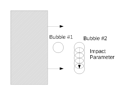
Figure 4.— Multiple bubbles with two bubbles and a varying impact parameter. We adjust the position of bubble #2 in increments of $R_{\text{bub}}$ while keeping the position of bubble #1 the same.

The second approach simulates three families each of 2, 4, or 8 non-overlapping bubbles, randomly placed in a box of volume $8^{3}R_{\text{bub}}^{3}$ with periodic boundary conditions along the $y$- and $z$-axes. Figure 5 provides before and after surface renderings of a simulation of a shock interacting with four bubbles.

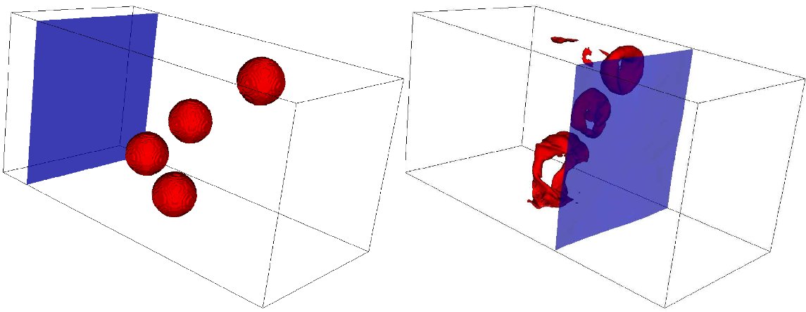
Figure 5.— Multiple bubbles with four bubbles randomly placed. At the far end of the box is a Mach 2 shock approaching the bubbles.

2.5.3 Resolution Study

To ensure that we have simulated the relevant dynamics and that numerical resolution effects did not influence our results, we performed a resolution study by increasing the refinement in our adaptive mesh, the results of which are presented in Figure 6.

It is clear from the figure that the value of $g$ determined from the simulation converges at a maximum refinement level of 5 at the surface of the bubble, i.e., at an effective resolution of 32 cells across the bubble. In other words, $g_{1}$ measured in our simulations is robust.

A high-resolution 2.5D axi- symmetric simulation in a uniform grid also shows excellent convergence with the 3D simulation at refinement level 5 and above, corresponding to a resolution of 32 cells across the bubble, as can be seen in Figure 11. The highest resolution simulations we ran of the Mach 2 case have an effective resolution of 128 cells across the bubble, corresponding to a numerical Reynolds number of order $Re\sim 10^{4}$. For low Mach numbers, we are therefore confident that our simulations fully resolve the gross vortex dynamics and that the numerical values we determine for $g_{1}$ are correct.

The situation changes at high Mach number: The highly turbulent and fragment flow around the Mach 8 vortex shown in Figure 10 exhibits structure all the way to the resolution limit and the vortex breaks apart (see discussion in §3.2 and 5).

In terms of the evolution of $g_{1}$, our resolution study shows that simulations at Mach numbers well above 2 have not converged, as might be expected from the degree of turbulence present in the flow and we limit discussion of these cases to a phenomenological description of the dynamics observed in our simulations for the interested reader, since higher resolution simulations would be computationally unfeasible given reasonable resources.

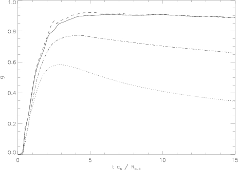
Figure 6.— Resolution study for a Mach 2 sphere. We represent maximum refinement levels of 3, 4, 5, and 6 with dotted, dot dashed, solid and dashed lines respectively. Level 5 appears to have the minimum necessary resolution to refine the relevant dynamics, corresponding to a resolution of 32 cells across the bubble.

3. The Efficiency of the Richtmyer-Meshkov Instability in 3D

Before discussing the relevance of vortex creation to the thermal evolution of galaxy clusters and AGN feedback, we will discuss our simulation results in the context of traditional fluid dynamics and compare them to experiments and previous theoretical and numerical work.

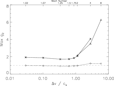
Figure 7.— RMI efficiency factor $g_{2}$ as a function of Mach number. The stars represent spheres, diamonds represent “infinite” cylinders, and triangles represent spheres in the 2.5D axi-symmetric simulations. The dashed line represents the approximation given by HC05, corresponding to the kinetic energy contained in a bubble of volume $V_{\rm bub}$ in the upstream/unshocked medium, as seen from the downstream/shocked frame.

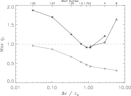
Figure 8.— RMI efficiency factor $g_{1}$ as a function of Mach number. Same symbols and Mach numbers as those in Figure 8. The dashed line represents the kinetic energy of a bubble with volume $V_{\text{bub}}$ in the downstream/shocked material, as seen from the upstream/unshocked frame.

Having introduced the RKE as a measure of the efficiency of the RMI in §2.3, we will first draw a comparison to the previous 2D results from HC05 and then discuss an extension of the investigation to a broader set of questions in a general fluid mechanics context, such as the non-linear interaction between vortices, and a comparison to previous studies.

3.1. Low Mach numbers

In their 2D investigation of the RMI, HC05 showed that, in 2D, vortex creation by the RMI can be surprisingly efficient, with $g_{2}\approx 1$ for bubbles much smaller than the depth $\lambda$ of the shock, but large compared to the shock thickness $\delta$. The efficiency depends on geometric factors, but HC05 showed that, over a range of Mach numbers from $M=1.01$ to $M=4$, the efficiency $g_{2}$ is independent of $M$.

However, as is well known in the case of other fluid processes, the behavior can be qualitatively different in three dimensions. The most obvious difference between the 2D and the 3D case is the fact that a spherical bubble has more surface area per volume, and a larger fraction of that surface area is oriented perpendicular to the shock normal.

Since vorticity is generated if and only if the baroclinic term $\nabla p\times\nabla\rho\not=0$ is non-vanishing, a larger fraction of bubble surface misaligned with the shock means a larger area over which the baroclinic term is non-vanishing. One should therefore expect a spherical (3D) bubble to have higher efficiency at generating vorticity than an infinite (2D) cylinder.

This can easily be verified from Fig. 7 which plots $g_{2}$ as a function of shock Mach number for spherical (3D) and cylindrical (2D) bubbles. Our 2D results reproduce the finding that $g_{2}=1$ for cylinders from HC05. For the spherical case, we find that $g_{2}\approx 2$ for Mach numbers smaller than $M<2$, confirming the significantly increased efficiency of the RMI in 3D.

For comparison, we have also plotted the peak value of $g_{1}$ in Figure 8. As expected, the two curves converge for low Mach numbers, where the shock compression ratio approaches unity.

3.2. High Mach numbers

For larger $M$, a second clear difference from 2D emerges: $g_{2}$ starts deviating significantly from a constant. The peak value of $g_{2}$ is strongly increased over $g_{2}=2$ at high Mach numbers. This occurs both in the full 3D simulations as well as in the 2.5D axi-symmetric simulations in the same geometry as the 3D case (i.e., a spherical bubble, triangles in Figures 7 and 8).

As expected for higher Mach number shocks, the increase in post-shock pressure implies that the vortex ring is becomes more strongly compressed, leading to the formation of a very thin vortex ring. Properly simulating the dynamics of such a ring requires a significantly higher maximum refinement level than is the case at low Mach numbers (see Table 1) and ultimately prohibited us from reaching convergence of our high Mach number simulations.

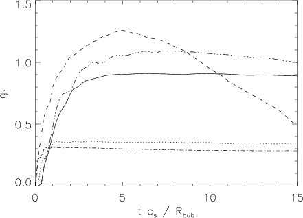
Figure 9.— $g_{1}$ vs. time for Mach 4 and Mach 8 simulations. The solid line represents a Mach 2 spherical bubble, the dash dot dotted line represents a Mach 4 spherical bubble, the dotted line represents a Mach 4 “infinite” cylinder, the short dashed line represents a Mach 8 spherical bubble with a maximum refinement level of 6, and the long dashed line represents a Mach 8 spherical bubble with a maximum refinement level of 7, and the dash dotted line represents a Mach 8 “infinite” cylinder.

In addition, the long term evolution of the vortex also changes at high Mach number, as shown in Figure 9. While in the $M<2$ case $g_{1}$ remains essentially constant for the entire duration of the simulation once the shock has crossed, $g_{1}$ shows a measurable decline in the Mach 4 case and an even more marked decline in the Mach 8 case, after reaching its significantly higher peak value. This behavior, however, is absent in the 2.5D case, as can be seen in the asymptotic behavior of $g_{1}$ in Figure 11.

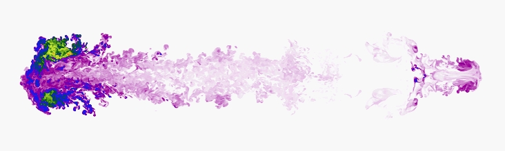
Figure 10.— Tracer fluid distribution for a full 3D Mach 8 simulation at $tc_{s}/R_{\text{bub}}\approx 12$. Note the high degree of complexity present in the flow, compared to the lower Mach number cases shown above.

The reason for the rapid decline in ordered vortex energy is the development of turbulence around the vortex, which completely disrupts the vortex ring fairly shortly after the shock crossing. This can be seen in Fig. 10, which shows the distribution of tracer fluid initially contained inside the bubble after $\sim 50$ shock crossing times. The vortex is completely disrupted and turbulence has cascaded down to the smallest resolved scales.

As stated in §2.5.3, our simulations are not fully resolving the flow at the highest Mach numbers and we will therefore defer a quantitative investigation of the efficiency of the high-Mach number RMI to future work.

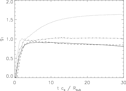
Figure 11.— $g_{1}$ vs. $t$ for spherical bubbles in a 2D axi-symmetric simulations. The dashed line represents a Mach 2 shock, the dash dotted line a Mach 4 shock, and the dotted line a Mach 8 shock. The solid line represents a spherical bubble with a Mach 2 shock in 3D.

3.3. The effects of geometry and non-linear vortex interactions on the RMI

Filamentary relativistic plasma in cluster atmospheres (as well as many other astrophysical objects) will often deviate from a purely spherical geometry. The increase in $g$ from 2D cylinders to 3D spheres demonstrates the effect of geometry on the efficiency of the RMI. Following HC05, we evaluated the dependence of $g$ on bubble aspect ratio and inclination.

Figure 12 shows that cylinders oriented perpendicular to the shock normal are less efficient than spheres (as already discussed above), and that cylinders oriented along the shock normal are more efficient. This makes intuitive sense, as vorticity generation is maximized when the portion of the bubble surface perpendicular to the pressure gradient is maximized.

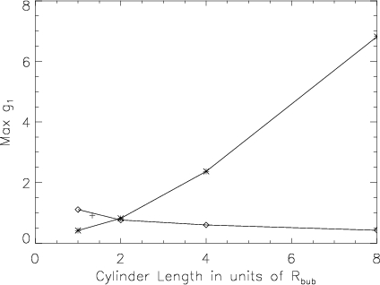
Figure 12.— Efficiency $g_{1}$ of the RMI for cylindrical bubbles of varying length and orientation for a Mach 2 shock, plotted against cylinder aspect ratio (length in units of radius). Cylinders perpendicular and parallel to the shock normal are shown as diamonds and stars, respectively. The cross indicates the value of $g_{1}$ for a spherical bubble.

It is reasonable to expect that $g$ should vary smoothly as we vary the inclination with the shock normal. This effect is shown in Fig. 13, along with an simple, ad-hoc parameterization as a sinusoid (in rough qualitative agreement with the data).

If we suppose that a sinusoid provides a good approximation and that a cylinder of aspect ratio $\mathcal{R}\gg 1$ has a minimum efficiency of $g_{2,{\rm min}}\approx 1$ and a maximum efficiency of $g_{2,{\rm max}}(\mathcal{R})$, the average efficiency for a randomly oriented set of filaments should be $\langle g_{2}\rangle\approx 0.5(0.5+g_{2,{\rm max}})$.

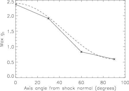
Figure 13.— Maximum $g_{1}$ value vs. axis angle of a cylinder from shock normal (degrees) for a Mach 2 shock. Cylinders have an axial length $L=4R_{\text{bub}}$. The dashed line is the curve given by $1.5+0.9\times\cos(\theta\pi/90)$.

The presence of multiple filaments or bubbles also implies that the individual vortices created in the interaction with a passing wave will interact with each other. Individual vortex velocity profiles can be expected to fall off roughly as $|v(r)|\propto r^{-3}$ with distance $r$ from the center at large $r\gg R$, where $R$ is the characteristic vortex size, (Batchelor, 1967; Heinz et al., 2011). Two vortices separated by a distance of order $R$ will interact strongly, while one can expect the interaction to be insignificant for large distances, given the steep dependence of $v$ or $r$.

We attempted to quantify this interaction with two numerical experiments. Figure 14 shows the results from the experiment described in Figure 4: two spherical bubbles placed behind each other with a varying lateral offset. Given the dependence of $g$ on cylinder inclination, one would expect an aligned configuration (with zero lateral offset) to have higher efficiency than a configuration in which two vortices are laterally offset by some impact parameter $b>0$.

This is supported by the simulations. For two aligned bubbles (with longitudinal offset of 4 bubble radii), the net efficiency is larger than for two individual bubbles, while the net efficiency is reduced for bubbles with a lateral offset. Figure 14 shows the temporal evolution of the interaction: As we reduce the impact parameter, the efficiency decreases from that of two isolated vortices as the inter-vortex interaction increases.

With increasing offset, the effect appears later and becomes weaker, as expected. At an impact parameter of 4 bubble radii, the result becomes virtually identical to the isolated case. This has implications for the effect of bubble filling factor on the efficiency $g$ of the RMI: For volume filling fractions below $\approx 2\%$, we expect relatively little non-linear interaction between vortices (corresponding roughly to the offset of 4 bubble radii both laterally and longitudinally for which we measured little effect on $g$), while for filling factors larger than about 2%, we should expect a measurable effect.

Since, on average, two randomly placed vortices will be aligned at an angle relative to the shock normal, this effect will reduce the average efficiency $g$. This can be seen in Fig. 15, which shows the results of our simulations of ensembles of randomly placed bubbles. The hatched areas plotted show the envelope of $g$ spanned by the different realizations for filling factors of 1.5%, 3%, and 6% as a function of time, compared to a single bubble. The presence of multiple bubbles reduces the peak efficiency and introduces a temporal decline not present in the simulations of individual bubbles at the same Mach number.

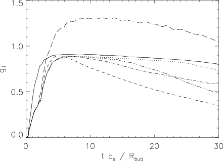
Figure 14.— Efficiency $g_{1}$ for two interacting bubbles, offset along the shock normal by 4 bubble radii and transverse to the shock normal by an increasing impact parameter for a Mach 2 shock; solid line: single bubble; long dashed: two bubbles, transverse offset $b=0{\,R_{\text{bub}}}$; short dashed: $b=1\,R_{\text{bub}}$; dash–dotted: $b=2\,R_{\text{bub}}$; dashed–triple–dotted: $b=3\,R_{\text{bub}}$; dotted: $b=4\,R_{\text{bub}}$.

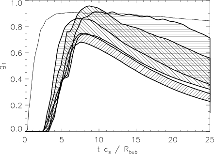
Figure 15.— $g$ vs. time for a Mach 2 shock with multiple, randomly placed bubbles (for the filling factors given below). Horizontally hatched: the two bubbles; upper-left to lower-right hatched: four bubbles; lower-left to upper-right: eight bubbles, compared to the single bubble case (thin solid line). The average filling factors for the different 2, 4, and 8 bubble realizations are approximately 1.5%, 3%, and 6% respectively.

3.4. Secondary effects

As discussed in HC05, the structure of the wave passing over a bubble and the density contrast affect the efficiency of the RMI. The bulk of the simulations in this paper were carried out under the assumption of having a small bubble radius compared to the pulse width of the shock (i.e., we simulated the shock as a semi-infinite piston) and a density contrast of 100.

3.4.1 Shock geometry

To investigate the effect of finite shock width on $g$, we injected a top-hat pressure and density perturbation (satisfying the shock jump conditions at the leading edge) to travel through the grid, with width, $\lambda\leq 2R$ (for $\lambda\gg R$, we expect the result of the semi-infinite piston to hold). The results are presented in Figs. 16 and 17.

As in the case of the non-linear interaction between vortices, $g_{1}$ reaches a peak value and declines as the inverted pressure gradient at the back of the perturbation reverses some of the vorticity generation of the shock. In the limit of narrow shocks (where the pulse width is small compared to the bubble size) we should expect that the peak in $g$ is significantly reduced compared to the semi-infinite piston case, as the shock has signficantly reduced energy compared to the maximum possible. This is borne out by the results shown in Fig. 16. Similar to the 2D case presented in HC05, smaller bubbles relative to the pulse width are more efficient at generating vorticity.

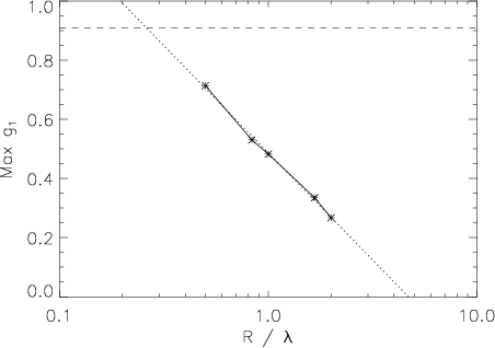
Figure 16.— $g_{1}$ as a function of pulse width for a Mach 2 top-hat shock. The dashed line represents a top-hat shock with infinite length or a infinitely long piston. The dotted line represents the fit to the data given by $g_{1}=0.49-0.31\times\ln({R_{\text{bub}}}/{\lambda})$.

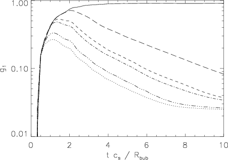
Figure 17.— $g_{1}$ as a function of time for a Mach 2 top-hat shock of width $\lambda=2R_{\text{bub}}$ (long dashed), $\lambda=1.2R_{\text{bub}}$ (short dashed), $\lambda=1.0R_{\text{bub}}$ (dash-dotted), $\lambda=0.6R_{\text{bub}}$ (dashed-triple-dotted), and $\lambda=0.5R_{\text{bub}}$ (dotted). The solid line represents the semi-infinite piston.

3.4.2 Density Contrast

The X-ray cavities in the centers of cool core clusters discussed in this paper are generally filled with radio synchrotron emitting plasma. While it is reasonable to assume that the density contrast between the radio plasma and the thermal ICM gas is very large (validating our choice of $\rho_{\rm bub}\ll\rho_{\rm ICM}$), the best observational upper limits of the filling fraction of thermal gas inside the bubbles are about an order or magnitude larger: Sanders & Fabian (2007) report an upper limit of 15% on the filling factor of thermal gas inside the inner cavities in the Perseus cluster at a temperature of 10 keV or below, which translates into a limit of $\rho_{\rm bub}/\rho_{\rm ICM}\leq 0.15$ assuming pressure equilibrium between the cavity and the surrounding ICM.

Since the efficiency of the RMI must approach zero as the density contrast approaches unity, we expect $g_{1}$ to decrease as $\rho_{\rm bub}/\rho_{\rm ICM}$ increases. In order to quantify this decrease, we ran a set of simulations spanning a range of $10^{-2}\leq\rho_{\rm bub}/\rho_{\rm ICM}\leq 0.5$. We plotted the resulting dependence of $g_{1}$ on the density contrast in Fig. 18. Given the upper limits on the filling factor of thermal gas inside cavities by Sanders & Fabian (2007), the effect of mixing in cluster will, at most, reduce the effect of the RMI on cavities by $\sim$30%. The dependence of $g$ on $\rho_{\rm buble}/\rho_{\rm ICM}$ is well fit by the ad-hoc expression

$$g_{1} =g_{\infty}\times e^{-4.32\times\rho_{\text{bubble}}/\rho_{\text{ICM}}} g_{\infty} =0.960$$ (11)

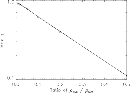
Figure 18.— $g_{1}$ as a function of bubble density contrast ($\rho_{\text{bub}}/\rho_{\text{ICM}}$) for a Mach 2 shock. Dashed line is the fit to the data as expressed in equation 11.

3.5. Placing This Investigation into a Broader Fluid Mechanics Context

We can derive a number of easily measurable quantities from our set of simulations that allow comparison to other studies in the fluid mechanics literature and are useful experimental diagnostics of the RMI.

3.5.1 Vortex velocities

When a shock encounters a bubble it creates at least one, often two, vortex rings. The upstream vortex, which contains most of the RKE, always forms and, following literature convention, we refer to this vortex as the primary vortex ring (PVR). A downstream/shocked vortex sometimes forms with a usually smaller radius, which we refer to as the secondary vortex ring (SVR). We can clearly see these vortex rings in Figure 3; at that time for the Mach 2 case, the SVR has just started to form, as noted by the curl-up downstream from the PVR.

We note that a SVR does not always occur in a sub-set of our simulations, in particular:

• at low Mach numbers ($M\lesssim 1.07$), mainly because it takes so long for vortices to form

• in the case of multiple bubbles

• in simulations of cylinders with axes parallel to the shock normal

• at high Mach numbers (e.g. Mach 8).

We track the locations and velocities of both PVR and SVR by finding the peak values of the tracer fluid (projected onto the vortex axis). Figure 19 shows the resulting locations for our fiducial Mach 2 simulation, indicating that the the SVR slowly drifts away from the PVR and that both move at near constant velocity.

In Fig. 20 we plot the best fit PVR velocities from linear regressions to the positions of the tracer maxima (the variance in $v_{\rm PVR}$ is reflected in the error bars). It is clear from the figure that the PVR generally slows down relative to the downstream/shocked velocity as the Mach number increases.

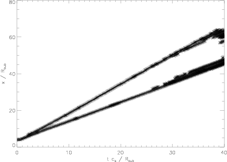
Figure 19.— Location of maxima in fluid tracer distribution vs. time for our fiducial Mach 2 run. Only those maxima with a maximum value with 3% of the global maximum for each time are plotted. The top line corresponds to the movement of the PVR, whereas the bottom line corresponds to the movement of the SVR.

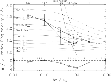
Figure 20.— Measured velocity of the primary vortex ring (triangles) as a function of Mach number, compared to the prediction from eq. (12) and the measured vortex radii $R_{\rm PVR}$ (stars). For comparison, the dashed line represents the speed of the shock front for a given $\Delta v$, whereas the the dashed-dotted line represents the upstream/unshocked sound speed, $c_{s}$. The bottom portion of the plot represents the difference between the two lines divided by the uncertainty of both curves added in quadrature.

Ranjan et al. (2008a, §VI) provide an analytic estimate of the velocity of the PVR as a function of the vortex ring radius $R_{\rm PVR}$, based on the model from Picone & Boris (1988).

$$\frac{v_{\text{PVR}}}{\Delta v} =1+\frac{R_{\text{PVR}}}{2\pi D_{V}}\left(1-\frac{\Delta v}{2Mc_{s}}\right)\ln\left(\frac{\rho_{\text{ICM}}}{\rho_{\text{bub}}}\right)$$ (12)

To compare our work to prior results (Ranjan et al., 2008a), we converted their data using eq. 12 for a fluid with adiabatic index $\gamma=5/3$ and a density contrast of $\rho_{\text{ICM}}/\rho_{\text{bub}}=100$ and measured radii $R_{\rm PVR}$ for the vortex rings for different Mach numbers.

This model provides a reasonable approximation for the PVR velocities for low Mach numbers, as shown in Fig. 20. The top panel of the figure shows the measured PVR velocity (triangles) and the predicted values from eq. (12).

To calculate the errors in $v_{\rm PVR}$, we selected points that belonged to the PVR in a figure like Fig. 19 and performed a linear regression of those points. From the fit, we obtain a slope and an error for our fit. To measure the ring radii, we performed a weighted average on the tracer fluid. The variance in these measurements is reflected in the error bars in the stars in Fig. 20.

In the lower panel of Fig. 20, we plot the difference between the model and the measurements for $v_{\rm PVR}$ ($\Delta$) divided by the estimated uncertainty ($\sigma$).

3.5.2 Vortex turnover locations and times

The time it takes for the vortex to form after the shock first encounters the bubble provides an important diagnostic, both astrophysically and in laboratory experiments.

The distance traveled by the shock at the time the vortex forms — the minimum stand-off distance between vortex and shock — provides another diagnostic that can be applied directly to astrophysical observations. The stand-off distance is also a direct measure of the vortex velocity relative to the shock velocity in the downstream frame.

The criterion for vortex formation in the simulations is most easily defined as the condition that a spine of high-density, shocked material passes all the way through the bubble. Technically, this criterion is satisfied when no more tracer fluid can be found along the axis.

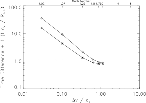
Figure 21.— Time elapsed between when shock front passes location where vortex will form and when the vortex forms. The dashed horizontal line represents when the shock front reaches the location of vortex formation at the time the vortex forms. Stars represent spheres and diamonds represent cylinders.

The turnover time is shown in Figure 21, measured in units of shock crossing times of the bubble.

A plot of the stand-off distance as a function of Mach number is shown in Fig. 22, in units of initial bubble radii. Given an observational estimate of the stand-off distance, it is possible to derive a lower limit on the Mach number from this figure, since the minimum stand-off distance decreases with increasing Mach number.

Figure 22.— Plot of the distance between shock front and vortex at the time of vortex formation. The dashed horizontal line represents when the shock front reaches the location of vortex formation at the time the vortex forms. Stars represent spheres and diamonds represent cylinders. Since the vortex, has to travel more slowly than the shock, this is the minimum distance that can be observed between a shock and a vortex.

4. Dissipation of wave energy in the intracluster medium

As originally suggested in HC05, the kinetic energy contained in the vortex field generated in the wake of a shock or steepened sound wave passing over filaments of hot/relativistic gas in galaxy cluster cores might be dissipated on time scales long compared to the shock passage time but short compared to the cluster cooling time. The presence of multiple generations of cavities of relativistic plasma in the cluster could thus enhance the dissipation of acoustic energy released by the generation of subsequent cavities through the activity of the AGN.

A vortex created by this process exhibits a differentially rotating velocity profile, which can be seen from the radial decline in the vortex energy density in Fig. 3. In the presence of microscopic or turbulent viscosity, the induced strain in the velocity field will ultimately lead to dissipation of the kinetic energy in the vortex.

Based on the results of our 3D parameter study of the efficiency of the RMI, we can estimate the dissipation rate for the vortex energy and determine under which conditions we might expect it to contribute significantly to the thermodynamics of the cluster gas.

4.1. Viscous Dissipation of Vortex Rings

As we discussed in §3.2, strong shocks generate vortices that are inherently dynamically unstable on a shock passage timescale. The vortex field generated by the shock thus dissipates in a turbulent cascade quickly after the shock passed, with high efficiency. Strong shocks are also inherently dissipative, and any region of the cluster subject to such a shock will be heated efficiently regardless of the presence or absence of the RMI.

However, given the well known evolution of expanding AGN driven cavities in clusters (e.g. Heinz et al., 1998), only a small volume and mass fraction of the cluster will be subject to such strong shocks, while most of the cluster only experiences relatively weak shocks, consistent with the observations of shock Mach numbers in the range of 1-2 in clusters where shocks have been discovered.

As demonstrated above, the vortices generated for such weak to moderate shocks are dynamically stable for times much longer than the shock crossing time, and the shock or sound wave itself will not contribute sufficiently to the heating of the gas to offset cooling unless the viscosity is close to the Spitzer value (Reynolds et al., 2005).

However, the vortex ring itself is differentially rotating. As originally suggested in HC05, viscous dissipation due to the shear in this flow will transfer some of the rotational kinetic energy in the vortex to heat in the cluster gas on a viscous dissipation time scale $\tau_{\rm diss}$.

It is easy to derive the natural scaling of $\tau_{\rm diss}$ with vortex parameters: Following equations 5 and 7, the vortex energy is given by $E_{\rm rot}=V_{\rm bubble}\rho_{2}\frac{(\Delta v)^{2}}{2}g_{1}$.

The characteristic velocity of the vortex is simply $\Delta v$; the velocity decreases from $\sim\Delta v$ outward from the vortex surface. It is clear that $\Delta v$ must be the velocity scale imposed by the initial conditions and our simulations confirm this (see Picone & Boris (1988); Batchelor (1967) for a more rigorous motivation).

The characteristic volume inside which most of the vortex is contained must be of the order of $V_{\rm bubble}$. Finally, the vortex must have a characteristic scale length of the order of the initial bubble radius, $r_{\text{bub}}$.

Consequently, the shear inside this volume is of the order of

$$\frac{\partial v_{\rm rot}}{\partial r}\sim\frac{\Delta v}{r_{\rm bubble}}$$ (13)

Following (Reynolds et al., 2005), we write the viscosity in terms of the Spitzer-Braginsky value (Braginskii, 1958; Spitzer, 1962)

$$\mu =2.21\times 10^{-15}\frac{T^{5/2}}{Z^{4}\ln\Lambda}\frac{\text{g}}{\text{cm s}}$$ (14)

$$=1.88\times 10^{3}T_{5}^{5/2}\text{g cm}^{-1}\text{ s}^{-1}$$

where we have introduced a fiducial cluster temperature of $kT=5T_{5}\text{ keV}$ and used $\ln\Lambda\approx 30$.

We also define a fractional viscosity parameter (i.e., the viscosity measured in units of the Spitzer value) as

$$f_{\rm Sp}\equiv\frac{\mu}{\mu_{\rm Spizter}}$$ (15)

The dissipation rate for a vortex with these characteristic parameters will then be of the order of

$$\left.\frac{dE}{dt}\right|_{\rm diss} = \int dV\Pi:\nabla\vec{v}$$ (16)

$$= \int dV\mu\left(\frac{\partial v_{i}}{\partial x_{j}}+\frac{\partial v_{j}}{\partial x_{i}}-\frac{2}{3}\nabla\cdot\vec{v}\right)$$

$$\times\left(\frac{\partial v_{i}}{\partial v_{j}}+\frac{\partial v_{j}}{\partial x_{i}}\right)$$

$$\equiv 2V_{\rm bubble}\mu\left(\frac{\Delta v}{R}\right)^{2}\xi_{\rm diss}$$ (18)

where we introduced the dissipation efficiency coefficient $\xi_{\rm diss}$, to be evaluated from the actual shear and vortex volume measured in the simulation.

The dissipation time, using eqs. 5 and 7, will then be of the order of

$$\tau_{\rm diss} \equiv \frac{E_{\rm rot}}{dE/dt}$$ (19)

$$\sim \frac{V_{\rm bubble}\rho_{2}\frac{(\Delta v)^{2}}{2}g_{1}}{\mu\frac{(\Delta v)^{2}}{R^{2}}V_{\rm bubble}}\xi_{\rm diss}^{-1}=\frac{R_{\text{bub}}^{2}g_{1}\rho_{2}}{2\mu\xi_{\rm diss}}$$ (20)

$$\sim 1.3\times 10^{6}\,{\rm yrs}\,\frac{R_{\rm kpc}^{2}\rho_{0.01}g_{1}}{f_{\rm Sp}T_{5}^{5/2}\xi_{\rm diss}}$$ (21)

which we use as our fiducial reference scale to plot the numerically determined dissipation rates against.

While our simulations were inviscid (with the exception of numerical viscosity and artificial viscosity employed in the shock-capturing scheme), we can calculate the viscous dissipation rate and thus $\xi_{\rm diss}$ a posteriori, using a finite-difference representation of eq. 4.1.

Our simulations approximate the relativistic, non-thermal plasma inside the vortex as hot, thermal gas. Given the steep temperature dependence in $\mu$, and given the high temperatures inside the vortex, care must be taken in excluding any contribution to the dissipation rate from inside the vortex itself, which would be unphysical.

To this end, we impose a temperature cutoff on the gas, motivated by the fact that the post-shock gas around the vortex occupies a relatively narrow range in temperature, clearly separate from the much hotter vortex. We chose a conservative cut of $T_{\rm cut}=1.25T_{2}$, which effectively excludes most of the hot vortex.

We performed this analysis on both the entire velocity field, $\mathbf{v}$, and just the rotational component of the velocity field, $\mathbf{v}_{R}$. If the analysis is limited to exclude the shock (which contributes to the viscous dissipation rate of the full velocity field but is naturally absent in the rotational component of the flow), we find that the late-time difference between the dissipation rates for the rotational and the full velocity field is less than 5%. This is consistent with the absence of any significant viscous dissipation in the acoustic part of the velocity field.

The viscous dissipation rate in units of $\left.dE/dt\right|_{\rm diss}$ from eq. (4.1 for different Mach numbers as a function of time is shown in Fig. 23. Figure 24 plots the inferred dissipation time in units of $\tau_{\rm diss}$ from eq. (21).

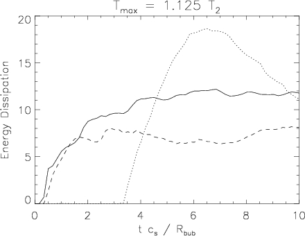
Figure 23.— Viscous Energy Dissipation Rate, $\xi_{\text{diss}}$, in units of the fiducial dissipation rate from eq. (4.1), plotted against simulation time in units of bubble sound crossing times. The solid line represents a Mach 2 shock interacting with a spherical bubble; the short dashed line corresponds to a Mach 1.5 shock, and the dotted line to a Mach 1.07 shock.

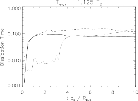
Figure 24.— Viscous Energy Dissipation Time in units of the fiducial dissipation time from eq. (21), equal to the ratio of the dimensionless factors $g_{1}/\xi_{\text{diss}}$ (same line styles as Fig. 23

As can be seen from Fig. 23, the dissipation rate inferred from strain and vortex volume measured in the simulations is about an order of magnitude larger than the natural scaling derived in eq. 4.1, i.e., $\xi_{\rm diss}\sim 10$, and we will use $\xi_{\rm diss}\equiv 10\xi_{10}$ as our fiducial value through the rest of the discussion. We attribute this to the fact that the velocity gradients inside the vortex are, in fact, significantly steeper and more concentrated than the simple estimate of $\Delta v/r_{\rm bubble}$ would suggest (which we confirmed by inspection of individual frames of the simulation).

This carries over to the estimated dissipation times of vortices in clusters, which is also about an order of magnitude shorter than the fiducial rate.

4.2. Application to Galaxy Clusters

The dissipation time should be compared to the residence time of the vortex (i.e., the travel time through the cooling region) and the cluster cooling time in order to assess the viability of this process to contribute to the thermalization of AGN energy in clusters. Technically, these depend on the cluster properties, but given that cooling times in the centers of cool core clusters are of the order of a few hundred million years.

Taking the viscous dissipation efficiency plotted in Fig. 24, and denoting the cooling function of the gas as $\Lambda(T)\equiv 10^{-23}\,{\rm ergs\,cm^{3}\,s^{-1}}\Lambda_{-23}(T)$, the cooling time is longer than the dissipation time if

$$\frac{\Lambda_{-23}(T)\,R_{\rm kpc}^{2}\,\rho_{0.01}^{2}g_{1}}{f_{\rm Sp}T_{5}^{7/2}}<3\times 10^{4}$$ (22)

If the dissipation time is long compared to the cooling time, an AGN driven feedback loop will not be able to counteract the onset of cooling rapidly enough to maintain thermal balance of the cluster. Whether the condition $\tau_{\rm diss}<\tau_{\rm cool}$ evaluation in equation 22 is satisfied (i.e., whether the onset of AGN activity occurs at high enough temperatures for dissipation in the IGM to be efficient) will depend on the details of gas supply to the black hole as a function of central cluster temperature, given the strong temperature sensitivity of eq. 22.

Note, however, that the condition $\tau_{\rm diss}<\tau_{\rm cool}$ is not a strict requirement for feedback to work, as long as a sufficient fraction of the vortex energy is dissipated in the cooling region to offset cooling in an average sense, as eventually, a sufficient amount of energy will be liberated by the AGN to counteract cooling.

A more important requirement for effective heating is that the vortex remain in the cluster core long enough to dissipate a significant fraction of its energy. The vortex residence time in the cluster is more difficult to estimate than the dissipation time: Our simulations are idealized in that they model the shock as a semi-infinite piston. And shocks and non-linear sound waves in clusters are impulsive, and thus the long term dynamics of the vortex might be different from our idealized simulations.

With this caveat in mind, we conservatively use our estimates of the primary vortex velocities from Fig. 20 to derive a rough estimate of the residence time. The figure shows that the velocity of the primary vortex ring (which contains the bulk of the vortex energy) travels at velocities between 1.4 and 2.5 times the velocity differential $\Delta v$, with vortices produced by weaker shocks traveling relatively faster compared to $\Delta v$.

While for strong shocks this implies that the vortex travels close to the shock speed (consistent with the fact that the standoff distance between vortex and shock can be very small, as seen in Fig. 22), for weaker shocks, the vortex travels significantly more slowly than the shock, which travels essentially at the sound speed, while $\Delta v$ is much smaller than $c_{\rm s}$.

From Fig. 20, we can see that the vortex velocity is smaller than the sound speed of the cluster for shocks with Mach number below about 1.6, with vortices created by weak shocks traveling at very sub-sonic speeds. For most of its propagation through a cluster, an AGN driven shock will be below this critical Mach number.

Taking the conservative upper limit on the PVR velocity to be about $v_{\rm PVR}\lesssim 2.5\Delta v$, the actual velocity through the ICM will be

$$\frac{v_{\rm PVR}}{c_{\rm s}} \lesssim 2.5\frac{\Delta v}{c_{\rm s}}=2.5\times\frac{3}{4}\left(M-\frac{1}{M}\right)$$ (23)

where $c_{\text{s}}$ is the upstream/unshocked sound speed and we have used $\gamma=5/3$ in calculating $\Delta v$ as a function of $M$.

For a cluster with cooling radius $r_{\rm cool}\equiv 50\,{\rm kpc}\,r_{50}$, the travel time through the cooling region is then

$$\tau_{\rm travel} \sim\frac{r_{\text{cool}}}{v_{\text{PVR}}}\sim\frac{r_{\rm cool}}{2.5c_{\rm s}}\frac{4}{3}\frac{M}{M^{2}-1}$$ (24)

$$\sim 2\times 10^{7}\,{\rm yrs}\frac{r_{50}}{T_{5}^{1/2}}\frac{M}{M^{2}-1}$$

and the dissipation time is smaller than the travel time if

$$\frac{R_{\rm kpc}^{2}\rho_{0.01}g_{1}}{f_{\rm Sp}T_{5}^{2}r_{50}\xi_{10}}\left(M-1/M\right)\lesssim 150$$ (25)

We can compare the viscous dissipation time to the eddy turnover time (i.e., the turbulent dissipation time),

$$\tau_{\rm turb}\sim\frac{R_{\rm bub}}{\Delta v}=7\times 10^{6}\,{\rm yrs}\frac{R_{\rm kpc}}{T_{5}^{1/2}\left(M_{1}-1/M_{1}\right)}$$ (26)

which is shorter than the viscous dissipation time if

$$\frac{f_{\rm Sp}T_{5}^{2}\xi_{10}}{R_{\rm kpc}\rho_{0.01}g_{1}\left(M_{1}-1/M_{1}\right)}\lesssim 0.02$$ (27)

which, not surprisingly, is the case for large bubbles and strong shocks.

Whether the dissipation of vortex energy contributes significantly to cluster heating will, of course, ultimately depend on the energy released by the AGN. Even if the dissipation time is short compared to the travel time and the cooling time, a sufficient amount of energy has to be injected into waves and then extracted into the vortex field, which depends on the filling factor of cavities in clusters and the on AGN energy output relative to the cooling rate.

As already shown in HC05, the attenuation length of a wave with width $\lambda\gg R_{\rm bubb}$ interacting with a field of underdense bubbles of filling factor $f$ is roughly

$$L\sim\frac{\lambda}{2g_{1}f}$$ (28)

where we have included the factor 2 increase in efficiency introduced by extending the analysis to 3D. For the wave to lose most of its energy within the cooling radius, the filling factor would have to be larger than

$$f\gtrsim\frac{10\%}{g_{1}}\left(\frac{50\,{\rm kpc}}{r_{\rm cool}}\frac{\lambda}{10\,{\rm kpc}}\right)$$ (29)

Given that all cool core clusters show clear evidence of bubbles, and in cases where statistics allow, multiple generations thereof, such large filling factors are not unreasonable and consistent with estimates of the amount of non-thermal pressure present in the ICM of nearby clusters.

While the uncertainty in the relevant parameters (namely, the distribution of $R_{\rm bubb}$ of radio plasma, and the filling factor $f$, the Spitzer fraction $f_{\rm SP}$) is too large to conclude that visco-rotational heating is an important contributor to the thermal evolution, the study shows that the process should be studied further: It is clear that it must happen at some level when AGN-driven waves pass over the existing pockets of radio plasma, and under the right conditions, it can be very important in the extraction of energy from sound and shock waves in clusters.

5. Conclusions

We presented a detailed numerical investigation of the efficiency of the Richtmyer-Meshkov instability in the context of shocks passing over radio plasma filaments and cavities in galaxy cluster atmospheres. We investigated the possibility that extraction and dissipation of energy from weak shocks and non-linear sound waves often found in the centers of cool core clusters could contribute significantly to the heating of cool core clusters.

We introduced a 3D solenoidal/Helmholtz decomposition as an analytic tool to study the efficiency of vortex generation and to quantify the energy deposited in the vortex field upon passage of the shock over a bubble.

We generally confirmed the previous calculations of HC05 in the 2D limit and extended the analysis to full 3D simulations. We found that, for roughly spherical bubbles, the efficiency of vortex generation, as measured by the kinetic energy in the vortex field, is increased by a factor of 2 over the 2D case.

In the case of high Mach numbers ($M\gtrsim 4$), we found that the simulated vortices are not stable and degenerate into turbulence. The vortex energy is quickly dissipated and the vortex shredded (this can be clearly seen from Figure 10). Generally, strong shocks are not observed in the centers of clusters ICM, so we should expect RMI generated vortices in cluster atmospheres to be stable, though this might not be the case in the very centers of clusters in the presence of powerful, young radio galaxies. Lastly, strong shocks will raise the temperature of the gas on their own can, eliminating the requirement for additional dissipation mechanisms to facilitate AGN energy deposition in response to cluster cooling.

We found that non-linear interactions of multiple vortices can dynamically disrupt the vortices, leading to enhanced dissipation and a rapid decline in the kinetic energy in the vortex field, similar to what is seen in the case of large Mach numbers. While further investigation of this effect is necessary, we speculate that this is similarly due to the development of turbulence, as was found in the 2D case of random two-phase gas distributions in HC05. As a result of this effect, the efficiency of vortex generation and dissipation will depend on the average distance between vortices, i.e., the volume filling factor of low density plasma, with values significantly in excess of a few % indicating strongly non-linear interaction between vortices.

Since the vortex is a differentially rotating flow, it must be subject to viscous dissipation. We found that viscous dissipation of the vortex is about an order of magnitude more efficient than would be expected from a simple dimensional scaling argument. We showed that the viscous dissipation time is shorter for smaller vortices (i.e., bubbles) and that, in general, it can be smaller than the cluster crossing time and the ICM cooling time for bubbles smaller than about 10 kpc if the viscosity is at the few percent level of the Spitzer value. Observations of the center of nearby clusters (Fabian et al., 2005; Forman et al., 2005; Young et al., 2002) indicate that the multi-phase gas in cluster centers might have the right properties for viscous dissipation to contribute to cluster heating.

For this process to be thermodynamically relevant to the ICM within the cooling radius, the filling factor of non-thermal plasma must be significant (again of the order of a few percent). An investigation of how the non-linear interaction of closely spaced vortices will affect the heating of the ICM via the RMI is beyond the scope of this paper.

In order to compare our results to the existing experimental and numerical body of work on the RMI, we examined the velocities of the vortex rings in our simulations. We found that the velocities of the primary vortex ring (PVR) roughly match those predicted by Picone & Boris (1988) and expressed in equation 12, with some significant deviations at intermediate Mach numbers.

Finally, we introduced a new diagnostic for constraining the Mach number of shock waves present in the ICM: The stand-off distance between shock and vortex (see Fig. 22). Since vortex formation is slower, relative to shock passage, for weaker shocks, an observed stand-off distance can provide a lower limit on the Mach number.

5.1. Acknowledgements

We would like to thank Mateusz Ruszkowski, Marcus Brüggen, Ellen Zweibel, Rich Townsend, Eric Wilcots, and Riccardo Bonazza for helpful comments and discussions. The software used in this work was in part developed by the DOE-supported ASC / Alliance Center for Astrophysical Thermonuclear Flashes at the University of Chicago. Thank you to the CHTC for computational resources. SH and SHF acknowledge support from NASA through Chandra theory grant TM9-0007X and from NSF through grant AST0707682.

References

- Bagabir & Drikakis (2001) Bagabir, A., & Drikakis, D. 2001, Shock Waves, 11, 209
- Balsara (1998) Balsara, D. S. 1998, ApJS, 116, 133
- Batchelor (1967) Batchelor, G. 1967, An Introduction To Fluid Dynamics (Cambridge University Press, Cambridge, UK)
- Begelman (2001) Begelman, M. C. 2001, in Astronomical Society of the Pacific Conference Series, Vol. 240, Gas and Galaxy Evolution, ed. J. E. Hibbard, M. Rupen, & J. H. van Gorkom, 363–+
- Blanton et al. (2009) Blanton, E. L., Randall, S. W., Douglass, E. M., Sarazin, C. L., Clarke, T. E., & McNamara, B. R. 2009, ApJ, 697, L95
- Blanton et al. (2001) Blanton, E. L., Sarazin, C. L., McNamara, B. R., & Wise, M. W. 2001, ApJ, 558, L15
- Braginskii (1958) Braginskii, S. I. 1958, Soviet Journal of Experimental and Theoretical Physics, 6, 358
- Brouillette (2002) Brouillette, M. 2002, Annual Review of Fluid Mechanics, 34, 445
- Churazov et al. (2000) Churazov, E., Forman, W., Jones, C., Böhringer, H. 2000, A&A, 356, 788
- Churazov et al. (2001) Churazov, E., Brüggen, M., Kaiser, C. R., Böhringer, H., & Forman, W. 2001, ApJ, 554, 261
- Colella & Woodward (1984) Colella, P., & Woodward, P. R. 1984, Journal of Computational Physics, 54, 174
- Dong & Stone (2009) Dong, R., & Stone, J. M. 2009, ApJ, 704, 1309
- Dubey et al. (2008) Dubey, A., Reid, L. B., & Fisher, R. 2008, Physica Scripta Volume T, 132, 014046
- Enßlin & Brüggen (2002) Enßlin, T. A., & Brüggen, M. 2002, MNRAS, 331, 1011
- Fabian et al. (2000) Fabian, A. C., Sanders, J. S., Ettori, S., Taylor, G. B., Allen, S. W., Crawford, C. S., Iwasawa, K., Johnstone, R. M., & Ogle, P. M. 2000, MNRAS, 318, L65
- Fabian et al. (2005) Fabian, A. C., Sanders, J. S., Taylor, G. B., & Allen, S. W. 2005, MNRAS, 360, L20
- Fabian et al. (2006) Fabian, A. C., Sanders, J. S., Taylor, G. B., Allen, S. W., Crawford, C. S., Johnstone, R. M., & Iwasawa, K. 2006, MNRAS, 366, 417
- Forman et al. (2005) Forman, W., Nulsen, P., Heinz, S., Owen, F., Eilek, J., Vikhlinin, A., Markevitch, M., Kraft, R., Churazov, E., & Jones, C. 2005, ApJ, 635, 894
- Forman et al. (2007) Forman, W., et al. 2007, ApJ, 665, 1057
- Friedman & Heinz (In Prep.) Friedman, S. H., & Heinz, S. In Prep., ApJS
- Fryxell et al. (2000) Fryxell, B., Olson, K., Ricker, P., Timmes, F. X., Zingale, M., Lamb, D. Q., MacNeice, P., Rosner, R., Truran, J. W., & Tufo, H. 2000, ApJS, 131, 273
- Gardini & Ricker (2004) Gardini, A., & Ricker, P. M. 2004, Modern Physics Letters A, 19, 2317
- Giordano & Burtschell (2006) Giordano, J., & Burtschell, Y. 2006, Physics of Fluids, 18, 036102
- Graham et al. (2008) Graham, J., Fabian, A. C., & Sanders, J. S. 2008, MNRAS, 386, 278
- Heinz et al. (2011) Heinz, S., Brüggen, M., & Friedman, S. 2011, ApJS, 194, 21
- Heinz et al. (2002) Heinz, S., Choi, Y., Reynolds, C. S., & Begelman, M. C. 2002, ApJ, 569, L79
- Heinz & Churazov (2005) Heinz, S., & Churazov, E. 2005, ApJ, 634, L141
- Heinz et al. (1998) Heinz, S., Reynolds, C. S., & Begelman, M. C. 1998, ApJ, 501, 126
- Jones & De Young (2005) Jones, T. W., & De Young, D. S. 2005, ApJ, 624, 586
- Klein et al. (1994) Klein, R. I., McKee, C. F., & Colella, P. 1994, ApJ, 420, 213
- Layes et al. (2005) Layes, G., Jourdan, G., & Houas, L. 2005, Physics of Fluids, 17, 028103
- Layes et al. (2009) —. 2009, Physics of Fluids, 21, 074102
- Liu et al. (2008) Liu, W., Li, H., Li, S., & Hsu, S. C. 2008, ApJ, 684, L57
- Mathews et al. (2006) Mathews, W. G., Faltenbacher, A., & Brighenti, F. 2006, ApJ, 638, 659
- McNamara & Nulsen (2007) McNamara, B. R., & Nulsen, P. E. J. 2007, ARA&A, 45, 117
- McNamara et al. (2005) McNamara, B. R., Nulsen, P. E. J., Wise, M. W., Rafferty, D. A., Carilli, C., Sarazin, C. L., & Blanton, E. L. 2005, Nature, 433, 45
- McNamara et al. (2000) McNamara, B. R., Wise, M., Nulsen, P. E. J., David, L. P., Sarazin, C. L., Bautz, M., Markevitch, M., Vikhlinin, A., Forman, W. R., Jones, C., & Harris, D. E. 2000, ApJ, 534, L135
- Meshkov (1969) Meshkov, E. E. 1969, Fluid Dynamics, 4, 101, 10.1007/BF01015969
- Million et al. (2010) Million, E. T., Werner, N., Simionescu, A., Allen, S. W., Nulsen, P. E. J., Fabian, A. C., Bohringer, H., & Sanders, J. S. 2010, ArXiv e-prints
- Morsony et al. (2010) Morsony, B. J., Heinz, S., Brüggen, M., & Ruszkowski, M. 2010, MNRAS, 407, 1277
- Niederhaus et al. (2008) Niederhaus, J. H. J., Greenough, J. A., Oakley, J. G., Ranjan, D., Anderson, M. H., & Bonazza, R. 2008, Journal of Fluid Mechanics, 594, 85
- O’Neill et al. (2009) O’Neill, S. M., De Young, D. S., & Jones, T. W. 2009, ApJ, 694, 1317
- Owen et al. (2000) Owen, F. N., Eilek, J. A., & Kassim, N. E. 2000, ApJ, 543, 611
- Pavlovski et al. (2008) Pavlovski, G., Kaiser, C. R., Pope, E. C. D., & Fangohr, H. 2008, MNRAS, 384, 1377
- Picone & Boris (1988) Picone, J. M., & Boris, J. P. 1988, Journal of Fluid Mechanics, 189, 23
- Quirk & Karni (1996) Quirk, J. J., & Karni, S. 1996, Journal of Fluid Mechanics, 318, 129
- Rafferty et al. (2006) Rafferty, D. A., McNamara, B. R., Nulsen, P. E. J., & Wise, M. W. 2006, ApJ, 652, 216
- Ranjan et al. (2007) Ranjan, D., Niederhaus, J., Motl, B., Anderson, M., Oakley, J., & Bonazza, R. 2007, Physical Review Letters, 98, 024502
- Ranjan et al. (2008a) Ranjan, D., Niederhaus, J. H. J., Oakley, J. G., Anderson, M. H., Bonazza, R., & Greenough, J. A. 2008a, Physics of Fluids, 20, 036101
- Ranjan et al. (2008b) Ranjan, D., Niederhaus, J. H. J., Oakley, J. G., Anderson, M. H., Greenough, J. A., & Bonazza, R. 2008b, Physica Scripta Volume T, 132, 014020
- Reynolds et al. (2005) Reynolds, C. S., McKernan, B., Fabian, A. C., Stone, J. M., & Vernaleo, J. C. 2005, MNRAS, 357, 242
- Richtmyer (1960) Richtmyer, R. D. 1960, Communications on Pure and Applied Mathematics, 13, 297
- Ruszkowski et al. (2007) Ruszkowski, M., Enßlin, T. A., Brüggen, M., Heinz, S., & Pfrommer, C. 2007, MNRAS, 378, 662
- Sanders & Fabian (2007) Sanders, J. S., & Fabian, A. C. 2007, MNRAS, 381, 1381
- Soker et al. (2009) Soker, N., Sternberg, A., & Pizzolato, F. 2009, in American Institute of Physics Conference Series, Vol. 1201, American Institute of Physics Conference Series, ed. S. Heinz & E. Wilcots, 321–325
- Spitzer (1962) Spitzer, L. 1962, Physics of Fully Ionized Gases, 2nd edn. (Interscience, New York)
- Sternberg & Soker (2008) Sternberg, A., & Soker, N. 2008, MNRAS, 389, L13
- Woodward & Colella (1984) Woodward, P., & Colella, P. 1984, Journal of Computational Physics, 54, 115
- Young et al. (2002) Young, A. J., Wilson, A. S., & Mundell, C. G. 2002, ApJ, 579, 560