Chaotic mixing and fractals in a geophysical jet current

Abstract

We model Lagrangian lateral mixing and transport of passive scalars in meandering oceanic jet currents by two-dimensional advection equations with a kinematic stream function with a time-dependent amplitude of a meander imposed. The advection in such a model is known to be chaotic in a wide range of the meander’s characteristics. We study chaotic transport in a stochastic layer and show that it is anomalous. The geometry of mixing is examined and shown to be fractal-like. The scattering characteristics (trapping time of advected particles and the number of their rotations around elliptical points) are found to have a hierarchical fractal structure as functions of initial particle’s positions. A correspondence between the evolution of material lines in the flow and elements of the fractal is established.

1 Introduction

Major western boundary currents in the ocean are meandering jets separating water masses with different physical and biogeochemical characteristics. The prominent examples are the Gulf Stream in the Atlantic Ocean and the Kuroshio in the Pacific Ocean. These and similar "heat engines" define the climate in large regions of the planet. Similar jets in the stratosphere play important role in transport and distribution of chemical substances. From the hydrodynamic point of view, they may be considered as jet flows with running waves of different wave lengths and phase velocities imposed. The simplest kinematic model of such a flow is a two-dimensional jet of an ideal fluid with a given velocity profile that is perturbed by an amplitude-modulated wave traveling from the west to the east. The problem of transport and mixing of passive scalars in meandering jets has been considered by many authors in the context of atmospheric and oceanic physics [1, 2, 3, 4, 5, 6, 7, 8].

The typical phase portrait (Fig. 1) consists of two chains of circulations with a zigzag-like jet between them and resembles the phase portrait of a particle in the field of two running waves. In the frame moving with the velocity of one of the waves, the problem is topologically equivalent to the motion of a periodically perturbed nonlinear physical pendulum that is known to demonstrate chaotic oscillations [9, 10]. Different aspects of chaotic mixing of passive particles in meandering jets in the atmosphere and the ocean have been studied in the papers [1, 2, 3, 4, 5, 6, 7, 8].

In the paper we focus on topological and statistical aspects of the chaotic transport and mixing in a specific kinematic model of an eastward meandering jet which has been introduced in Refs. [2, 3] some years ago. We are motivated by the desire to get a more deep insight into the evolution of material lines in the flow and to establish a connection between dynamical, topological and statistical characteristics of the flow. The equations of motion of passive particles advected by a planar incompressible flow is known to have a Hamiltonian form

$$\dot{x} =u(x,y,\,t)=-\frac{\partial\Psi}{\partial y},$$ (1)

$$\dot{y} =v(x,y,\,t)=\frac{\partial\Psi}{\partial x},$$

with the streamfunction $\Psi$ playing the role of a Hamiltonian and the coordinates $(x,y)$ of a particle being canonically conjugated variables. Thus, nonstationary two-dynamical advection is equivalent to a Hamiltonian system with one and half degrees of freedom whose phase space coincides with its configuration space. This property is very useful in visualizing geometric invariant sets in real and numerical experiments.

2 Model flow

To be specific we consider a two-dimensional Bickley jet with the velocity profile $u_{0}\operatorname{sech}^{2}y$ whose argument is modulated by a zonal running wave [3]. The streamfunction in the fixed frame reference is the following:

$$\psi^{\prime}(x^{\prime},y^{\prime},\tau)=-\psi_{0}\tanh{\left(\frac{y^{\prime}-a\cos{k(x^{\prime}-c\tau)}}{\lambda\sqrt{1+k^{2}a^{2}\sin^{2}{k(x^{\prime}-c\tau)}}}\right)},$$ (2)

where $a$, $k$ and $c$ are amplitude, wavenumber and phase velocity respectively, $\lambda$ is a measure of the jet’s width. After introducing the following notations:

$$x =k(x^{\prime}-c\tau), y =ky^{\prime}, t =\psi_{0}k^{2}\tau,$$ (3)

$$x^{\prime} =\frac{x}{k}+c\tau, y^{\prime} =\frac{y}{k}, \tau =\frac{t}{\psi_{0}k^{2}}.$$

and

$$A=ak,\qquad L=\lambda k,\qquad C=\frac{c}{\psi_{0}k},$$ (4)

we get the advection equations (1) in the frame moving with the phase velocity $c$:

$$\begin{aligned} \dot{x}&=\frac{1}{L\sqrt{1+A^{2}\sin^{2}x}\cosh^{2}\theta}-C,\\ \dot{y}&=-\frac{A\sin x(1+A^{2}-Ay\cos x)}{L\left(1+A^{2}\sin^{2}x\right)^{3/2}\cosh^{2}\theta},\end{aligned}\qquad\theta=\frac{y-A\cos x}{L\sqrt{1+A^{2}\sin^{2}x}}.$$ (5)

Figure 1: Streamlines of the unperturbed system (5) in the frame moving with the meander’s phase velocity $c$.

The respective streamfunction

$$\psi(x,y)=-\tanh{\left(\frac{y-A\cos x}{L\sqrt{1+A^{2}\sin^{2}x}}\right)}+Cy$$ (6)

has three normalized control parameters: $L$, $A$ and $C$ are the jet’s width, meander’s amplitude and its phase velocity. The scaling chosen results in translational invariance of the phase portrait along the $x$-axis with the period $2\pi$.

The detailed analysis of stationary points and bifurcations of Eqs. (5) has been done in Ref. [11]. Stationary points may exist only under the condition $LC\leqslant 1$. There are four stationary points, two of them are always stable and the other ones are stable under the condition $AL\operatorname{Arcosh}\sqrt{1/LC}>1$. If the additional condition $C<1/L\cosh^{2}(1/AL)$ is fulfilled, there are additional four unstable saddle points. Resuming one gets:

1. $C>C_{\text{cr1}}=1/L$, there are no stationary points.

2. $C_{\text{cr1}}>C>C_{\text{cr2}}=1/L\cosh^{2}(1/AL)$ and $C>C_{\text{cr3}}$, there are two centers and two saddles with two separatrices connecting the saddles. There are two separatrices each of which passes through its own saddle. The jet between the separatrices is westward.

3. $C_{\text{cr1}}>C>C_{\text{cr2}}$ and $C<C_{\text{cr3}}$, the jet is eastward with the same stationary points as in the case 2.

4. $C_{\text{cr2}}>C>C_{\text{cr3}}$, there are eight stationary points and two separatrices. There are two separatrices, each of which connects two saddle points. The jet is westward.

5. $C_{\text{cr2}}>C$ and $C<C_{\text{cr3}}$, the jet is eastward with the same stationary points as in the case 4.

Therefore, from the point of view of existence and stability of stationary states, there are three possibilities: 1) there are no stationary points; 2) there are four stationary points, two centers and two saddles; 3) there are eight stationary points, four centers and four saddles. A bifurcation between the first and second regimes consists in arising two pairs ‘‘saddle-center’’. A bifurcation between the second and third regimes consists in arising two saddles and a center between them instead of one saddle (a fork-type bifurcation).

There is one more bifurcation that does not change the number and stability of stationary points but changes the topology of the flow. The values of the streamfunction on the separatrices are equal on modulo but of opposite signs. There is a critical value of the phase velocity $C=C_{\text{cr3}}$ under which the separatrices coincide and the respective streamfunction is equal to zero. If $C>C=C_{\text{cr3}}$, a free flow between the separatrices is westward, whereas with $C<C=C_{\text{cr3}}$ it is eastward. It is difficult to find $C=C_{\text{cr3}}$ analytically but it may be shown [11] that $C_{\text{cr3}}>C_{\text{cr2}}$, if

$$\frac{2(1+A^{2})}{AL\sinh(2/AL)}<1.$$ (7)

Otherwise $C_{\text{cr3}}<C_{\text{cr2}}$.

The respective phase portraits are typical with Hamiltonian systems with running waves in shear flows [6, 12]. In dependence on the values of the phase velocity $C$ one can get different topologies: a homoclinic connection, a heteroclinic connection and a separatrix reconnection. Being motivated by eastward jet currents in the ocean and atmosphere, we deal in this paper with the case 3 (see the phase portrait in Fig. 1).

3 Chaotic mixing and transport

Streamlines with the streamfunction (6), that is time-independent in the moving frame, are shown in Fig. 1. The plot demonstrates three different regions of the flow: a central eastward jet (J), north and south circulations (C) and peripheral westward currents (P). The centers of the circulations are at critical lines to be defined by the condition $u(y_{c})=c_{x}$, $v(y_{c})=0$, and they are divided by two separatrices connecting saddle points. No exchange between the north and south circulations is possible in the unperturbed system.

Even the simplest periodic perturbation of the meander’s amplitude, $A=A_{0}+\varepsilon\cos(\omega t+\varphi)$, results in spitting stable and unstable manifolds of the saddle points. There arise stochastic layers with chaotic mixing and transport of water masses fluxes of which depend on the width of a layer, a number of overlapping resonances and other factors. As an example, we plot in Fig. 2 the Poincaré section of the perturbed flow. The control parameters throughout the paper are chosen as follows: $A=0.785$, $C=0.1168$, $L=0.628$, $\varepsilon=0.0785$, $\omega=0.2536$ and $\varphi=\pi/2$.

Figure 2: General view of the Poincaré section of the system with a periodically modulated meander’s amplitude.

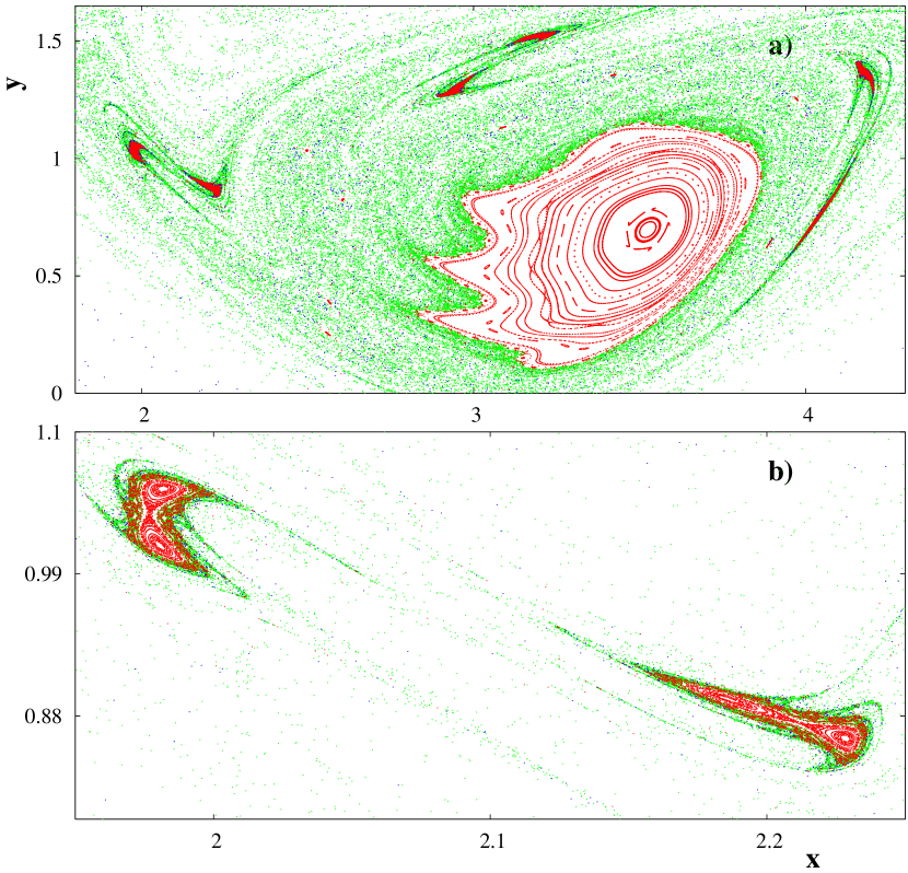
Figure 3: (a) Poincaré sections in the northern part of the first eastern frame, (b) stickiness to the island’s border.

Due to the zonal and meridian symmetries it is enough to consider mixing in the northern part of the first eastern frame only $0\leqslant x\leqslant 2\pi$. In Fig. 3a we plot the respective Poincaré section. The vortex core, that survives under the perturbation, is immersed into a stochastic sea where one can see 6 small islands belonging to the same resonance. Particles, belonging to these islands, rotate around the elliptic point of the vortex core. Zoom of the section nearby two of the islands is shown in Fig. 3b. The feature we want to pay attention to is a stickiness to the boundaries of the vortex core and of the islands that is visualized by increasing the density of points near the respective boundaries. It is a typical phenomenon with Hamiltonian systems [10] which influences essentially the transport of passive particles.

Figure 4: (a) Probability distribution functions (PDFs) of lengths of eastward (triangles) and westward (squares) flights obtained with $10$ chaotic trajectories for $5\cdot 10^{6}$ steps. The parameters are: $\varepsilon=0.0785$ and $\omega=0.2536$. (b) For short eastward flights, $12\leqslant x_{f}\leqslant 90$, the PDF decays exponentially. (c) The tails of both the PDFs decay as a power law with the slope $\nu=1.94\pm 0.09$ obtained with westward (squares) long flights $|x_{f}|>25$.

Without perturbation, the transport properties are very simple: particles either rotate in circulations C or move eastward in the jet J and westward in the peripheral currents P. Under a perturbation, the motion in the stochastic layers become extremely sensitive to small variations in initial conditions, and one is forced to use an statistical approach to describe transport. A commonly used statistical measure of transport is the variance $\sigma^{2}(t)=<x^{2}>$, where the averaging is supposed to be done over an ensemble of particles. Long time behavior of $\sigma^{2}(t)$ and of the probability density function of particle’s displacement $P(x,t)$ may be anomalous with typical chaotic Hamiltonian systems [13]. When $\sigma^{2}(t)\sim t$ and $P(x,t)$ is a Gaussian distribution, the advection is known to be normal with a well-defined diffusion coefficient $D=\lim_{t\to\infty}\sigma^{2}/2t$. When $\sigma^{2}(t)\sim t^{\gamma}$, with $\gamma\neq 1$, $D$ is either zero or infinite [13], and one gets either subdiffusion ($\gamma<1$) or super-diffusion ($\gamma>1$). If the trajectories are dominated by sticking regions nearby boundaries of islands, where particles spend a long time, subdiffusion results. Superdiffusion occurs when particles in the jet travel long distances between sticking events. The respective length and time PDFs are expected to be non Gaussian.

We will call ‘‘a flight’’ any event between two successive changes of signs of the particle’s zonal velocity. In this terminology a sticking consists of a number of flights with approximately equal flight times. The Poincaré section of the flow with the perturbation strength $\varepsilon=0.0785$ and frequency $\omega=0.2536$ is shown in Fig. 3a. The flight PDFs are computed with $10$ particles (initially placed in the first east frame inside a stochastic layer) up to the time $t=5\cdot 10^{6}$. The PDF of the lengths of flights is shown in Fig. 4a for both the directions. The asymmetry between the eastward (‘‘positive’’) and westward (‘‘negative’’) flights is evident. Both the PDFs can be roughly split into three distinctive regions. The very short flights with small values of $|x_{f}|$ ($<2\pi$) are supposed to be dominated by sticking to the boundaries of the vortex core and oscillatory islands. The PDF for eastward flights with the lengths in the range $12\leqslant x_{f}\leqslant 90$ decays exponentially (Fig. 4b). The tails of both the PDFs are close to a power-law decay $P(x_{f})\sim|x_{f}|^{-\nu}$. In Fig. 4c we estimate the exponent for long westward flights, $|x_{f}|>25$, with corresponding error by least-square fitting of the straight line to the log-log plot of the data to be $\nu=1.94\pm 0.09$.

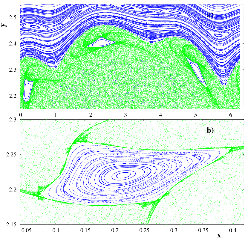
Figure 5: (a) The northern border between the circulation (C) and the peripheral current (P), (b) stickiness to the border of a ballistic island.

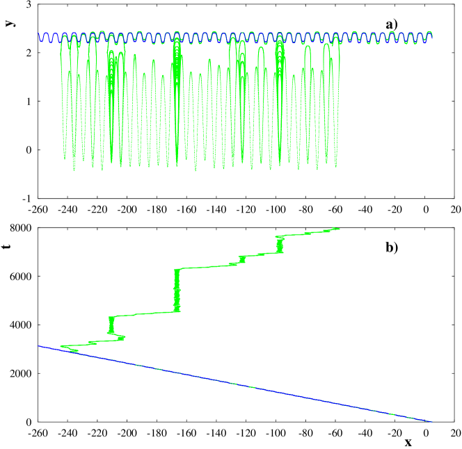
Figure 6: Examples of ballistic trajectories: the blue and regular trajectory, which is the upper one in (a) and the lower one in (b), is inside a ballistic island, the green and weakly chaotic trajectory, which is the lower one in (a) and the upper one in (b), is just outside the island. (a) $x-y$ plane, (b) dependence of the zonal position on time. Stickiness and flight events are evident with the green chaotic trajectory.

Besides resonant islands with particles moving around the elliptic point in the same frame (Fig. 3), we have found so-called ballistic islands which were situated both in the chaotic sea and in the peripheral jets (Fig. 5a). Ballistic modes [10, 14, 15] correspond to the stable periodic motion of particles from one frame to another. Particles, belonging to a ballistic island, move with a constant zonal velocity from one frame to another. When mapping their positions at the moments $t=2k\pi/\omega$ $(k=1,2,\dots)$ onto the first frame, we see a chain of islands which are visible in Fig. 5a. In Fig. 5b a zoom of the ballistic island is shown. Stickiness to the island’s border is evident. In Fig. 6 we demonstrate two ballistic trajectories corresponding to the ballistic island shown in Fig. 5b. If a particle at $t=0$ is placed inside the island, it travels to the west in a regular way (the upper blue trajectory in Fig. 6a). Its zonal position $x$ grows linearly with time (the lower blue trajectory in Fig. 6b). The lower green trajectory in Fig. 6a corresponds to a particle placed initially nearby the border of the same ballistic island from outside. Intermittent flight and sticking events are evident in Fig. 6b (the upper green curve in that figure).

4 Fractal geometry of mixing

Figure 7: Fractal set of initial positions $y_{0}$ of particles that reach the lines $x=0,\pm 2\pi$ after $n/2$ turns around the elliptic points. $T$ is a time particles need to reach the lines $x=0,\pm 2\pi$. Indices $e$ and $w$ mean particles moving in the eastward and westward directions, respectively.

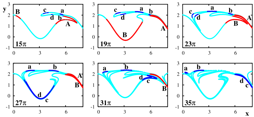
Figure 8: Fragments of the evolution of a material line in the first eastern frame. The fragments of the fractal in Fig. 7 with $n_{e}=1,2,3$ are marked by the respective letters.

Poincaré sections provide good impression about the structure of the phase space but not about geometry of mixing. In this section we consider the evolution of a material line consisting of a large number of particles distributed initially on a straight line that transverses the stochastic layer at $x=0$. A typical stochastic layer consists of an infinite number of unstable periodic and chaotic orbits with islands of regular motion to be imbeded. All the unstable invariant sets are known to possess stable and unstable manifolds. When time progresses particle’s trajectories nearby a stable manifold of an invariant set tend to approach the set whereas the trajectories close to an unstable manifold go away from the set. Because of such a very complicated heteroclinic structure, we expect a diversity of particle’s trajectories. Some of them are trapped forever in the first eastern frame $0\leqslant x\leqslant 2\pi$ rotating around the elliptic point along heteroclinic orbits. Other ones quit the frame through the lines $x=0$ or $x=2\pi$, and then either are trapped there or move to the neighbor frames (including the first one), and so on to infinity.

To get a more deep insight into the geometry of chaotic mixing we follow the methodology of our works [16, 17] and compute the time $T$, particles spend in the neighbor circulation zones $-2\pi\leqslant x\leqslant 2\pi$ before reaching the critical lines $x=0,x=\pm 2\pi$, and the number of times $n/2$ they wind crossing the lines $x=\pm\pi$. In the upper panel in Fig. 7 the functions $n(y_{0})$ and $T(y_{0})$ are shown. The upper parts of each function (with $n>0$ and $T>0$) represent the results for the particles with initial positive zonal velocities which they have simply due to their locations on the material line at $x=0$. These particles enter the eastern frame and may change the direction of their motion many times before leaving the frame through the lines $x=0$ or $x=2\pi$. The time moments of those events we fix for all the particles with $1.9\leqslant y_{0}\leqslant 2.045$. The lower "negative" parts of the functions $n(y_{0})$ and $T(y_{0})$ represent the results for the particles with initial negative zonal velocities ($y_{0}\geqslant 2.045$) which move initially to the first western frame ($-2\pi\leqslant x\leqslant 0$). In fact, $T_{e}(y_{0})$ and $T_{w}(y_{0})$ are the time moments when a particle with the initial position $y_{0}$ quits the eastern or western frames, respectively. Both the functions consist of a number of smooth U-like segments intermittent with poorly resolved ones. Border points of each U-like segments separate particles belonging to stable and unstable manifolds of the heteroclinic structure. The corresponding initial $y$-positions is a set (of zero measure) of particles to be trapped forever in the respective frame. A fractal-like structure of chaotic advection in both the frames is shown in the upper panel in Fig. 7, and its fragments for the first levels are shown in the middle panel for the eastern and the western fragments separately. Particles with even values of $n$ quit one the frames through the border $x=0$, those with odd $n$ – through the border $x=2\pi$ for the eastern frame and $x=-2\pi$ for the western one.

Let us consider in detail the fractal-like structure in the eastern frame keeping in mind that the results are similar with any other frame. The $n_{e}(y_{0})$-dependence is a complicated hierarchy of sequences of segments of the material line. Following to the authors of the paper [18], we call as an epistrophe a sequence of segments of the $(n+1)$-level, converging to the ends of a segment of a sequence of the $n$-th level, whose length decrease in accordance with a law. At $n_{e}=1$ we see in Fig. 7 an epistrophe with segment’s length A, B, C, D and so on decreasing as $l_{m}=l_{0}q^{m}$ with $q\approx 0.46$. Letters a and b in Fig. 7 denote the first segments of the epistrophes at the level $n_{e}=2$, whereas d and c —the first segments of the epistrophes at the level $n_{e}=3$. The respective laws for all those epistrophes are not exponential.

In Fig. 8 we demonstrate fragments of the evolution of the material line in the first eastern frame at the moments indicated in the figure. Letters on the line mark the corresponding segments of the $n_{e}(y_{0})$ and $T_{e}(y_{0})$ functions in Fig. 7. As an example, let us explain formation of the epistrophe ABCD at the level $n_{e}=1$. With the period of perturbation $T_{0}=2\pi/\omega\simeq 8\pi$, a portion from the north end of the material line leaves the frame through its eastern border. Look at the segments A and B at $t=15\pi$ and $t=23\pi$. They quit the first frame as a fold through the period $T_{0}\simeq 8\pi$. The other segments – C, and D (not shown in Fig. 8) do the same job. The epistrophe’s segments at the odd levels ($n=2k-1>1$) quit the frame with the period of perturbation $T_{0}$ one by one being folded (c and d segments). The folds of the segments of the $(2k-1)$-level are exterior with respects to the folds of the segments of the $(2k+1)$-level. The following empirical law is valid: $T_{2k-1}-T_{2k+1}\simeq 2T_{0}$, where $T_{2k-1}$ is a time when the first segments of the epistrophes at the level $(2k-1)$ (A with $n_{e}=1$) reach the line $x=2\pi$, and $T_{2k+1}$ the respective time for the first segments of the epistrophes at the level $2k+1$ (c and d segments with $n_{e}=3$).

Segments of the epistrophes of the even levels ($n=2k$) leave the frame with the period $T_{0}$ as well but through the border $x=0$ moving to the west. We show the evolution of some of them at the moments $t=31\pi$ and $t=35\pi$ in Fig. 8. Thus, the material line evolves by stretching and folding, and folds quit the frame in both directions with the period of perturbation.

5 Conclusion

We have treated the problem of mixing and transport of passive particles in a kinematic model of a meandering oceanic jet current from the point of view of dynamical system’s theory. A careful simulation of the Hamiltonian equations of advection has shown a complicated character of mixing under a time-dependent perturbation of the meander’s parameters. Both the oscillatory and ballistic resonant islands and sticking of trajectories to their boundaries have been found. The transport has benn shown to be anomalous. The geometry of mixing has been shown to be fractal-like. The trapping time of advected particles and the number of their rotations around elliptical points have been found to have a hierarchical fractal structure as functions of initial particle’s positions. A correspondence between the evolution of material lines in the flow and elements of the fractal has been established.

6 Acknowledgments

This work was supported by the Russian Foundation for Basic Research (Project no.06-05-96032), by the Program ‘‘Mathematical Methods in Nonlinear Dynamics’’ of the Russian Academy of Sciences and by the Program for Basic Research of the Far Eastern Division of the Russian Academy of Sciences.

References

- [1] J. Sommeria, S.D. Meyers, Y.L. Swinney, Laboratory model of a planetary eastward jet, Nature, 337 (1989) 58–62.
- [2] A.S. Bower, A simple kinematic mechanism for mixing fluid parcels across a meandering jet, J. Phys. Oceanogr., 21 (1989) 173-180.
- [3] R.M. Samelson, Fluid exchange across a meandering jet, J. Phys. Oceanogr., 22 (1992) 431–440.
- [4] T.H. Solomon, E.R. Weeks, H.L. Swinney, Observation of anomalous diffusion and Levy flights in a two-dimensional rotating flow, Phys. Rev. Lett., 71 (1993) 3975–3978.
- [5] D. Del-Castillo-Negrete, P.J. Morrison, Chaotic transport by Rossby waves in shear flow, Phys. Fluids A, 5 (1993) 948–965.
- [6] J.B. Weiss, E. Knobloch, Mass transport by modulated traveling waves, Phys. Rev.A., 42 (1989) 2579–2589.
- [7] K. Ngan, T. Shepherd, Chaotic mixing and transport in Rossby-wave critical layers, J. Fluid Mech., 334 (1997) 315–351.
- [8] J.Q. Duan, S. Wiggins, Fluid exchange across a meandering jet with quasi-periodic time variability, J. Phys. Oceanogr., 26 (1996) 1176-1188.
- [9] B.V. Chirikov, A universal instability of many-dimensional oscillator systems, Phys. Rep., 52 (1979) 263–379.
- [10] G.M. Zaslavsky, Hamiltonian Chaos and Fractional Dynamics, Oxford, Oxford University Press, 2005.
- [11] M.Yu. Uleysky, M.V. Budyansky, S.V. Prants, Chaotic advection in a meandering jet current, Nonlinear Dynamics, 1 (2006) is.2 [in Russian].
- [12] J.E. Howard, S.M Hohs, Stochasticity and reconnection in Hamiltonian systems, Phys. Rev.A, 29 (1984) 418–421.
- [13] M.F. Shlesinger, G.M. Zaslavsky, J. Klafter, Strange kinetics, Nature, 363 (1993) 31–38.
- [14] V. Rom-Kedar and G. Zaslavsky, Chaos, 9 (1999) 697–705.
- [15] A. Iomin, D. Gangardt, and S. Fishman, Phys. Rev. E. 57,(1998) 4054–4062.
- [16] M. Budyansky, M. Uleysky, S. Prants, Hamiltonian fractals and chaotic scattering by a topographical vortex and an alternating current, Physica D, 195 (2004) 369-378.
- [17] M.V. Budyansky, M.Yu. Uleysky, S.V. Prants, Chaotic scattering, transport, and fractals in a simple hydrodynamic flow, Zh. Eksp. Teor. Fiz., 126 (2004) 1167-1179 [JETP, 99 (2004) 1018-1027].
- [18] K.A. Mitchell, J.P. Handley, B. Tighe, J.B. Delos and S.K. Knudson, Geometry and topology of escape, Chaos, 13 (2003) 880-891.