The next-to-leading order forward jet vertex in the small-cone approximation

D.Yu. Ivanov^2¶ and A. Papa^1‡

¹ Dipartimento di Fisica, Università della Calabria,

and Istituto Nazionale di Fisica Nucleare, Gruppo collegato di Cosenza,

Arcavacata di Rende, I-87036 Cosenza, Italy

² Sobolev Institute of Mathematics and Novosibirsk State University,

630090 Novosibirsk, Russia

We consider within QCD collinear factorization the process $p+p\to{\rm jet}+{\rm jet}+X$, where two forward high-$p_{T}$ jets are produced with a large separation in rapidity $\Delta y$ (Mueller-Navelet jets). In this case the (calculable) hard part of the reaction receives large higher-order corrections $\sim\alpha^{n}_{s}(\Delta y)^{n}$, which can be accounted for in the BFKL approach. In particular, we calculate in the next-to-leading order the impact factor (vertex) for the production of a forward high-$p_{T}$ jet, in the approximation of small aperture of the jet cone in the pseudorapidity-azimuthal angle plane. The final expression for the vertex turns out to be simple and easy to implement in numerical calculations.

$\begin{array}[]{ll}{}^{\P}\mbox{{\it e-mail address:}}&\mbox{d-ivanov@math.nsc.ru}\\ {}^{\ddagger}\mbox{{\it e-mail address:}}&\mbox{papa@cs.infn.it}\\ \end{array}$

1 Introduction

The production of two forward high-$p_{T}$ jets in the fragmentation region of two colliding hadrons at high energies, the so called Mueller-Navelet jets [1], is considered an important process for the manifestation of the BFKL [2] dynamics at hadron colliders, such as Tevatron and LHC.

The theoretical investigation of this process implies a combined use of collinear and BFKL factorization: the process is started by two hadrons each emitting one parton, according to its parton distribution function (PDF), which obeys the standard DGLAP evolution [3]. On the other side, at large squared center of mass energy $\sqrt{s}$, i.e. when the rapidity gap between the two produced jets is large, the BFKL resummation comes into play, since large logarithms of the energy compensate the small QCD coupling and must be resummed to all orders of perturbation theory.

The BFKL approach provides a general framework for this resummation in the leading logarithmic approximation (LLA), which means resummation of all terms $(\alpha_{s}\ln(s))^{n}$, and in the next-to-leading logarithmic approximation (NLA), which means resummation of all terms $\alpha_{s}(\alpha_{s}\ln(s))^{n}$. Such resummation is process-independent and is encoded in the Green’s function for the interaction of two Reggeized gluons. The Green’s function is determined through the BFKL equation, which is an iterative integral equation, whose kernel is known at the next-to-leading order (NLO) both for forward scattering (i.e. for $t=0$ and color singlet in the $t$-channel) [4, 5] and for any fixed (not growing with energy) momentum transfer $t$ and any possible two-gluon color state in the $t$-channel [6].

The process-dependent part of the information needed for constructing the cross section for the production of Mueller-Navelet jets is contained in the impact factors for the transition from the colliding parton to the forward jet (the so called “jet vertex”).

Such impact factors were calculated with NLO accuracy in [7], where a careful analysis was performed, based on the separation of the various rapidity regions and on the isolation of the collinear divergences to be adsorbed in the renormalization of the PDFs. The results of [7] were then used in [8] for a numerical estimation in the NLA of the cross section for Mueller-Navelet jets at LHC and for the analysis of the azimuthal correlation of the produced jets. This numerical analysis followed previous ones [9, 10] based on the inclusion of NLO effects only in the Green’s functions. Recently we performed a new calculation [11] of the jet impact factor, confirming the results of  [7].

In this paper we recalculate the NLO impact factor for the production of forward jets in the “small-cone” approximation (SCA) [12, 13], i.e. for small jet cone aperture in the rapidity-azimuthal angle plane. Our starting point are the totally inclusive NLO parton impact factors calculated in [14], according to the general definition in the BFKL approach given in Ref. [15]. The calculation is lengthy, but straightforward, since the standard BFKL definition of impact factor provides the route to be followed. The use of the SCA, moreover, allows to get a simple analytic result for the jet vertices, easily implementable in numerical calculations and therefore particularly suitable for a semi-analytical cross-check of the numerical approaches which treat the cone size exactly.

The paper is organized as follows. In the next Section we will present the factorization structure of the cross section, recall the definition of BFKL impact factor and discuss the treatment of the divergences arising in the calculation; in Section 3 we describe the procedure for the jet definition and the SCA; in Section 4 and 5 we present the details of the calculation at LO and NLO, respectively; in Section 6 we draw some conclusions.

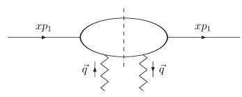
Figure 1: Diagrammatic representation of the forward parton impact factor.

2 General framework

We consider the process

$$p(p_{1})+p(p_{2})\to{\rm jet}(k_{1})+{\rm jet}(k_{2})+X\$$ (1)

in the kinematical region where the jets have large transverse momenta, $\vec{k}_{1}^{\,2}\sim\vec{k}_{2}^{\,2}\gg\Lambda_{\rm QCD}^{2}$. This provides the hard scale, $Q^{2}\sim\vec{k}_{1,2}^{\,2}$, which makes perturbative QCD methods applicable. Moreover, the energy of the proton collision is assumed to be much bigger than the hard scale, $s=2p_{1}\cdot p_{2}\gg\vec{k}_{1,2}^{\,2}$.

We consider the leading behavior in the $1/Q$-expansion (leading twist approximation). With this accuracy one can neglect the masses of initial protons. The state of the jets can be described completely by their (pseudo)rapidities $y_{1,2}$ and transverse momenta $\vec{k}_{1,2}$. Moreover, we denote the azimuthal angles of the jets as $\phi_{1,2}$.

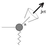
Figure 2: Parton-Reggeon collision, the jet is formed by a single parton.

In QCD collinear factorization the cross section of the process reads

$$\frac{d\sigma}{dy_{1}dy_{2}d^{2}\vec{k}_{1}d^{2}\vec{k}_{2}}=\sum_{i,j=q,g}\int\limits^{1}_{0}\int\limits^{1}_{0}dx_{1}dx_{2}f_{i}(x_{1},\mu_{F})f_{j}(x_{2},\mu_{F})\frac{d\hat{\sigma}(x_{1}x_{2}s,\mu_{F})}{dy_{1}dy_{2}d^{2}\vec{k}_{1}d^{2}\vec{k}_{2}}\;,$$ (2)

where the $i,j$ indices specify parton types, $i,j=q,\bar{q},g$, $f_{i}(x,\mu_{F})$ are the proton PDFs, the longitudinal fractions of the partons involved in the hard subprocess are $x_{1,2}$, $\mu_{F}$ is the factorization scale and $d\hat{\sigma}(x_{1}x_{2}s,\mu_{F})$ is the partonic cross section for the jet production.

It is convenient to define the Sudakov decomposition for the jet momenta,

$$k_{1}=\alpha_{1}p_{1}+\frac{\vec{k}^{\,2}_{1}}{\alpha_{1}s}p_{2}+k_{1,\,\perp}\ ,\quad k_{1,\,\perp}^{2}=-\vec{k}_{1}^{\,2}\ ,$$ (3)

$$k_{2}=\frac{\vec{k}^{\,2}_{2}}{\alpha_{2}s}p_{1}+\alpha_{2}p_{2}+k_{2,\,\perp}\ ,\quad k_{2,\,\perp}^{2}=-\vec{k}_{2}^{\,2}\ ,$$

where the jet longitudinal fractions $\alpha_{1,2}$ are related to the jet rapidities by

$$y_{1}=\frac{1}{2}\ln\frac{\alpha^{2}_{1}s}{\vec{k}^{\,2}_{1}}\ ,\quad y_{2}=-\frac{1}{2}\ln\frac{\alpha^{2}_{2}s}{\vec{k}^{\,2}_{2}}\,,$$ (4)

and $dy_{1}=\frac{d\alpha_{1}}{\alpha_{1}}$, $dy_{2}=-\frac{d\alpha_{2}}{\alpha_{2}}$ in the center of mass system.

We consider the kinematics when the interval of rapidity between the two jets,

$$\Delta y=y_{1}-y_{2}=\ln\frac{\alpha_{1}\alpha_{2}s}{|\vec{k}_{1}||\vec{k}_{2}|}\ ,$$ (5)

is large. Since the jet longitudinal fractions are equal or smaller (in the case of additional QCD radiation) than the ones of the participating partons, $\alpha_{1}\leq x_{1}$, $\alpha_{2}\leq x_{2}$, we are in a situation where the energy of the partonic subprocess is much larger than jet transverse momenta, $x_{1}x_{2}s\gg\vec{k}^{\,2}_{1,2}$ ($\vec{k}^{\,2}_{1}$ and $\vec{k}^{\,2}_{2}$ are considered to be of similar order $\sim\vec{k}^{\,2}$). In this region the perturbative partonic cross section receives at higher orders large contributions $\sim\alpha^{n}_{s}\ln^{n}\frac{s}{\vec{k}^{\,2}}$, related with large energy logarithms. It is the aim of this paper to elaborate the resummation of such enhanced contributions with NLA accuracy using the BFKL approach.

Let us remind some generalities of the BFKL method. Due to the optical theorem, the cross section is related to the imaginary part of the forward proton-proton scattering amplitude,

$$\sigma=\frac{{\cal I}m_{s}A}{s}\ .$$ (6)

In the BFKL approach the kinematic limit $s\gg\vec{k}^{\,2}$ of the forward amplitude may be presented in $D$ dimensions as follows:

$${\cal I}m_{s}\left({\cal A}\right)=\frac{s}{(2\pi)^{D-2}}\int\frac{d^{D-2}\vec{q}_{1}}{\vec{q}_{1}^{\,\,2}}\Phi_{1}(\vec{q}_{1},s_{0})\int\frac{d^{D-2}\vec{q}_{2}}{\vec{q}_{2}^{\,\,2}}\Phi_{2}(-\vec{q}_{2},s_{0})\int\limits^{\delta+i\infty}_{\delta-i\infty}\frac{d\omega}{2\pi i}\left(\frac{s}{s_{0}}\right)^{\omega}G_{\omega}(\vec{q}_{1},\vec{q}_{2})\,,$$ (7)

where the Green’s function obeys the BFKL equation

$$\omega\,G_{\omega}(\vec{q}_{1},\vec{q}_{2})=\delta^{D-2}(\vec{q}_{1}-\vec{q}_{2})+\int d^{D-2}\vec{q}\,K(\vec{q}_{1},\vec{q})\,G_{\omega}(\vec{q},\vec{q}_{1})\;.$$ (8)

What remains to be calculated are the NLO impact factors $\Phi_{1}$ and $\Phi_{2}$ which describe the inclusive production of the two jets, with fixed transverse momenta $\vec{k}_{1}$, $\vec{k}_{2}$ and rapidities $y_{1}$, $y_{2}$, in the fragmentation regions of the colliding protons with momenta $p_{1}$ and $p_{2}$, respectively. The energy scale parameter $s_{0}$ is arbitrary, the amplitude, indeed, does not depend on its choice within NLA accuracy due to the properties of NLO impact factors to be discussed below.

For definiteness, we will consider the case when the jet belongs to the fragmentation region of the proton with momentum $p_{1}$, i.e. the jet is produced in the collision of the proton with momentum $p_{1}$ off a Reggeon with incoming (transverse) momentum $q$ and denote for shortness in what follows its transverse momentum and longitudinal fraction by $\vec{k}$ and $\alpha$, respectively.

Technically, this is done using as starting point the definition of inclusive parton impact factor, given in Ref. [14], for the cases of incoming quark(antiquark) and gluon, respectively (see Fig. 1). Here we review the important steps and give the formulae for the LO parton impact factors.

Note that both the kernel of the equation for the BFKL Green’s function and the parton impact factors can be expressed in terms of the gluon Regge trajectory,

$$j(t)\;=\;1\>+\>\omega(t)\;,$$ (9)

and the effective vertices for the Reggeon-parton interaction.

To be more specific, we will give below the formulae for the case of forward quark impact factor considered in $D=4+2\epsilon$ dimensions of dimensional regularization. We start with the LO, where the quark impact factors are given by

$$\Phi_{q}^{(0)}(\vec{q}\,)\;=\;\sum_{\{a\}}\>\int\>\frac{dM_{a}^{2}}{2\pi}\>\Gamma_{aq}^{(0)}(\vec{q}\,)\>[\Gamma_{aq}^{(0)}(\vec{q}\,)]^{*}\>d\rho_{a}\;,$$ (10)

where $\vec{q}$ is the Reggeon transverse momentum, and $\Gamma^{(0)}_{aq}$ denotes the Reggeon-quark vertices in the LO or Born approximation. The sum $\{a\}$ is over all intermediate states $a$ which contribute to the $q\rightarrow q$ transition. The phase space element $d\rho_{a}$ of a state $a$, consisting of particles with momenta $\ell_{n}$, is ($p_{q}$ is initial quark momentum)

$$d\rho_{a}\;=\;(2\pi)^{D}\>\delta^{(D)}\left(p_{q}+q-\sum_{n\in a}\ell_{n}\right)\>\prod_{n\in a}\>\frac{d^{D-1}\ell_{n}}{(2\pi)^{D-1}2E_{n}}\;,$$ (11)

while the remaining integration in (10) is over the squared invariant mass of the state $a$,

$$M_{a}^{2}\;=\;(p_{q}+q)^{2}\;.$$

In the LO the only intermediate state which contributes is a one-quark state, $\{a\}=q$. The integration in Eq. (10) with the known Reggeon-quark vertices $\Gamma_{qq}^{(0)}$ is trivial and the quark impact factor reads

$$\Phi_{q}^{(0)}(\vec{q}\,)\;=g^{2}\frac{\sqrt{N^{2}-1}}{2N}\;,$$ (12)

where $g$ is QCD coupling, $\alpha_{s}=g^{2}/(4\pi)$, $N=3$ is the number of QCD colors.

In the NLO the expression (10) for the quark impact factor has to be changed in two ways. First one has to take into account the radiative corrections to the vertices,

$$\Gamma_{qq}^{(0)}\to\Gamma_{qq}=\Gamma_{qq}^{(0)}+\Gamma_{qq}^{(1)}\;.$$

Secondly, in the sum over $\{a\}$ in (10), we have to include more complicated states which appear in the next order of perturbative theory. For the quark impact factor this is a state with an additional gluon, $a=qg$. However, the integral over $M_{a}^{2}$ becomes divergent when an extra gluon appears in the final state. The divergence arises because the gluon may be emitted not only in the fragmentation region of initial quark, but also in the central rapidity region. The contribution of the central region must be subtracted from the impact factor, since it is to be assigned in the BFKL approach to the Green’s function. Therefore the result for the forward quark impact factor reads

$$\Phi_{q}(\vec{q}\,,s_{0})=\left(\frac{s_{0}}{\vec{q}^{\>2}}\right)^{\omega(-\vec{q}^{\>2})}\>\sum_{\{a\}}\>\int\>\frac{dM_{a}^{2}}{2\pi}\>\Gamma_{aq}(\vec{q}\,)\>[\Gamma_{aq}(\vec{q}\,)]^{*}\>d\rho_{a}\>\theta(s_{\Lambda}-M_{a}^{2})$$

$$-\frac{1}{2}\int d^{D-2}k\frac{\vec{q}^{\,\,2}}{\vec{k}^{\,2}}\Phi_{q}^{(0)}(\vec{k})\mathcal{K}_{r}^{(0)}(\vec{k},\vec{q}\,)\ln\left(\frac{s_{\Lambda}^{2}}{(\vec{k}-\vec{q}\,)^{2}s_{0}}\right)\;.$$ (13)

The second term in the r.h.s. of Eq. (2) is the subtraction of the gluon emission in the central rapidity region. Note that, after this subtraction, the intermediate parameter $s_{\Lambda}$ in the r.h.s. of Eq. (2) should be sent to infinity. The dependence on $s_{\Lambda}$ vanishes because of the cancellation between the first and second terms. $K_{r}^{(0)}$ is the part of LO BFKL kernel related to real gluon production,

$$K_{r}^{(0)}(\vec{k},\vec{q}\,)\;=\;\frac{2g^{2}N}{(2\pi)^{D-1}}\frac{1}{(\vec{k}-\vec{q}\,)^{2}}\;.$$ (14)

The factor in Eq. (2) which involves the Regge trajectory arises from the change of energy scale ($\vec{q}^{\>2}\to s_{0}$) in the vertices $\Gamma$. The trajectory function $\omega(t)$ can be taken here in the one-loop approximation ($t=-\vec{q}^{\,\,2}$),

$$\omega(t)\;=\;\frac{g^{2}t}{(2\pi)^{D-1}}\frac{N}{2}\int\frac{d^{D-2}k}{\vec{k}^{2}(\vec{q}-\vec{k})^{2}}\;=\;-\;g^{2}N\frac{\Gamma(1-\varepsilon)}{(4\pi)^{D/2}}\frac{\Gamma^{2}(\varepsilon)}{\Gamma(2\varepsilon)}(\vec{q}^{\,\,2})^{\varepsilon}\;.$$ (15)

In the Eqs. (10) and (2) we suppress for shortness the color indices (for the explicit form of the vertices see [14]). The gluon impact factor $\Phi_{g}(\vec{q}\,)$ is defined similarly. In the gluon case only the single-gluon intermediate state contributes in the LO, $a=g$, which results in

$$\Phi_{g}^{(0)}(\vec{q}\,)\;=\frac{C_{A}}{C_{F}}\Phi_{q}^{(0)}(\vec{q}\,)\;,$$ (16)

here $C_{A}=N$ and $C_{F}=(N^{2}-1)/(2N)$. Whereas in NLO additional two-gluon, $a=gg$, and quark-antiquark, $a=q\bar{q}$, intermediate states have to be taken into account in the calculation of the gluon impact factor.

The definition of inclusive parton impact factors involves the integration over all possible intermediate states appearing in the parton-Reggeon collision. Up to the next-to-leading order, this means that we can have one or two partons in the intermediate state. Then, in order to allow for the inclusive production of a jet, these integrations must be suitably constrained to take into account that the kinematics of the parton or the pair of partons which generate the jet is fixed by the jet kinematics.

3 Jet definition and small-cone approximation

At LO the (totally inclusive) parton impact factor takes contribution from a one-particle intermediate state; equivalently, only one parton is produced in the collision between the incoming parton and the Reggeon, as shown in Fig. 2. Therefore, the kinematics of the produced parton is totally fixed by the jet kinematics. At NLO we have both the virtual corrections (which have the kinematical structure shown in Fig. 2) and also two-particle production in the parton-Reggeon collision. The jet in the latter case can be either produced by one of the two partons or by both together. If we call the produced partons $a$ and $b$, we have the following contributions, as shown in Fig. 3 (see, for instance, Ref. [16]):

1. the parton $a$ generates the jet, while the parton $b$ can have arbitrary kinematics, provided that it lies outside the jet cone;

2. similarly with $a\leftrightarrow b$;

3. the two partons $a$ and $b$ both generate the jet.

The cases 1. and 2. are replaced in the actual calculation by the following two (as illustrated in Fig. 4):

1. the parton $a$ generates the jet, while the parton $b$ can have arbitrary kinematics (“inclusive” jet production by the parton $a$); then, the case when the parton $b$ lies inside the jet cone is subtracted;

2. similarly with $a\leftrightarrow b$.

Let us introduce now the “small-cone” approximation (SCA). In view of the discussion above, we should define it in the two cases of jet generated by one parton or by two partons.

The relative rapidity and azimuthal angle between the two partons are

$$\Delta y=\frac{1}{2}\ln\frac{\zeta^{2}(\vec{k}-\vec{q})^{2}}{\bar{\zeta}^{2}\vec{k}^{\,2}}\;,\;\;\;\;\;\Delta\phi=\arccos\frac{\vec{q}\cdot\vec{k}-\vec{k}^{\,2}}{|\vec{k}||\vec{q}-\vec{k}|}\;,\;\;\;\;\;\bar{\zeta}\equiv 1-\zeta\;.$$

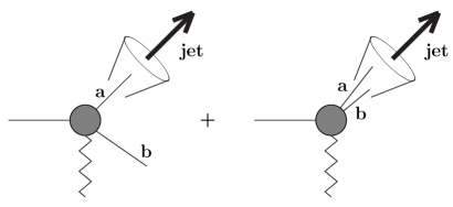
Figure 3: Parton-Reggeon collision, two partons are produced and the jet is formed either by one of the partons or by both partons.

Let the parton with momentum $\vec{k}$ and longitudinal fraction $\zeta$ generate the jet, whereas the other parton (with momentum $\vec{q}-\vec{k}$ and longitudinal fraction $\bar{\zeta}$) is a spectator. We introduce the vector $\vec{\Delta}$ such that

$$\vec{q}=\frac{\vec{k}}{\zeta}+\vec{\Delta}\;.$$

Then, for $\vec{\Delta}\to 0$ we have

$$\Delta\phi^{2}=\frac{\zeta^{2}}{\bar{\zeta}^{2}}\left(\frac{\vec{\Delta}^{2}}{\vec{k}^{\,2}}-\frac{(\vec{k}\cdot\vec{\Delta})^{2}}{\vec{k}^{\,4}}\right)\;,\;\;\;\;\;\Delta y=\frac{\zeta}{\bar{\zeta}}\frac{(\vec{k}\cdot\vec{\Delta})}{\vec{k}^{\,2}}\;,$$

thus the condition of cone with aperture smaller than $R$ in the rapidity-azimuthal angle plane becomes

$$\Delta\phi^{2}+\Delta y^{2}=\frac{\zeta^{2}}{\bar{\zeta}^{2}}\frac{\vec{\Delta}^{2}}{\vec{k}^{2}}\leq R^{2}$$

and therefore

$$|\vec{\Delta}|\leq\frac{\bar{\zeta}}{\zeta}|\vec{k}|R\;.$$

The situation is different when both partons form a jet. In this case the jet momentum is $\vec{k}=\vec{k}_{1}+\vec{k}_{2}$ and the jet fraction is $1=\zeta+\bar{\zeta}$. The relative rapidity and azimuthal angle between the jet and the first (second) parton are

$$\Delta y_{1}=\frac{1}{2}\ln\frac{\vec{k}_{1}^{\,2}}{\zeta^{2}\vec{k}^{\,2}}\;,\;\;\;\;\;\Delta\phi_{1}=\arccos\frac{\vec{k}\cdot\vec{k}_{1}}{|\vec{k}_{1}||\vec{k}|}\;,$$

$$\Delta y_{2}=\frac{1}{2}\ln\frac{(\vec{k}_{1}-\vec{k})^{2}}{\bar{\zeta}^{2}\vec{k}^{\,2}}\;,\;\;\;\;\;\Delta\phi_{2}=\arccos\frac{\vec{k}\cdot(\vec{k}-\vec{k}_{1})}{|\vec{k}||\vec{k}-\vec{k}_{1}|}\;.$$

Introducing now the vector $\vec{\Delta}$ as

$$\vec{k}_{1}=\zeta\vec{k}+\vec{\Delta}\;,$$

we find

$$\Delta y_{1}^{2}+\Delta\phi_{1}^{2}=\frac{\vec{\Delta}^{2}}{\zeta^{2}\vec{k}^{\,2}}\;,\;\;\;\;\;\Delta y_{2}^{2}+\Delta\phi_{2}^{2}=\frac{\vec{\Delta}^{2}}{\bar{\zeta}^{2}\vec{k}^{\,2}}\;,$$

so that the requirement that both partons are inside the cone is now

$$|\vec{\Delta}|\leq R\,|\vec{k}|\,\min(\zeta,\bar{\zeta})\;.$$

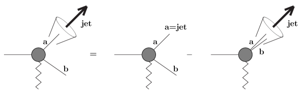
Figure 4: The production of the jet by one parton when the second one is outside the cone can be seen as the “inclusive” production minus the contribution when the second parton is inside the cone.

4 Impact Factor in the LO

The inclusive LO impact factor of proton may be thought of as the convolution of quark and gluon impact factors, given in Eqs. (12,16), with the corresponding proton PDFs,

$$d\Phi={\cal C}\,dx\left(\frac{C_{A}}{C_{F}}f_{g}(x)+\sum_{a=q,\bar{q}}f_{a}(x)\right)\ ,\quad{\cal C}=g^{2}\frac{\sqrt{N^{2}-1}}{2N}=2\pi\alpha_{s}\sqrt{\frac{2\,C_{F}}{C_{A}}}\;.$$ (17)

In order to establish the proper normalization for the jet impact factor, we insert into the inclusive impact factor (17) the delta functions which depend on the jet variables, transverse momentum $\vec{k}$ and longitudinal fraction $\alpha$:

$$\frac{d\Phi^{J}}{\vec{q}^{\,\,2}}={\cal C}\int\,d\alpha\frac{d^{2}\vec{k}}{\vec{k}^{\,2}}\,dx\,\delta^{(2)}\left(\vec{k}-\vec{q}\right)\delta(\alpha-x)\left(\frac{C_{A}}{C_{F}}f_{g}(x)+\sum_{a=q,\bar{q}}f_{a}(x)\right)\;.$$ (18)

In what follows we will calculate the projection of the impact factor on the eigenfunctions of LO BFKL kernel, i.e. the impact factor in the so called $(\nu,n)$-representation,

$$\Phi(\nu,n)=\int d^{2}\vec{q}\,\frac{\Phi(\vec{q})}{\vec{q}^{\,\,2}}\frac{1}{\pi\sqrt{2}}\left(\vec{q}^{\,\,2}\right)^{i\nu-\frac{1}{2}}e^{in\phi}\;.$$ (19)

Here $\phi$ is the azimuthal angle of the vector $\vec{q}$ counted from some fixed direction in the transverse space.

5 NLO calculation

We will work in $D=4+2\epsilon$ dimensions and calculate the NLO impact factor directly in the $(\nu,n)$-representation (19), working out separately virtual corrections and real emissions. To this purpose we introduce the “continuation” of the LO BFKL eigenfunctions to non-integer dimensions,

$$\left(\vec{q}^{\,\,2}\right)^{\gamma}e^{in\phi}\to\left(\vec{q}^{\,\,2}\right)^{\gamma-{n\over 2}}\left(\vec{q}\cdot\vec{l}\,\,\right)^{n}\;,$$ (20)

where $\gamma=i\nu-\frac{1}{2}$ and $\vec{l}^{\>2}=0$. It is assumed that the vector $\vec{l}$ lies only in the first two of the $2+2\epsilon$ transverse space dimensions, i.e. $\vec{l}=\vec{e}_{1}+i\,\vec{e}_{2}$, with $\vec{e}_{1,2}^{\>2}=1$, $\vec{e}_{1}\cdot\vec{e}_{2}=0$. In the limit $\epsilon\to 0$ the r.h.s. of Eq. (20) reduces to the LO BFKL eigenfunction. This technique was used recently in Ref. [17]. An even more general method, based on an expansion in traceless products, was uses earlier in Ref. [18] for the calculation of NLO BFKL kernel eigenvalues. In the case of interest, $\vec{l}^{\>2}=0$, these two approaches lead, actually, to similar formulas.

Thus, for the case of non-integer dimension the LO result for the impact factor reads

$$\frac{d\Phi^{J}}{\vec{q}^{\,\,2}}={\cal C}\,d\alpha\frac{d^{2+2\epsilon}\vec{k}}{\vec{k}^{\,2}}\,\delta^{(2+2\epsilon)}\left(\vec{k}-\vec{q}\right)\left(\frac{C_{A}}{C_{F}}f_{g}(\alpha)+\sum_{a=q,\bar{q}}f_{a}(\alpha)\right)\;,$$ (21)

which in the $(\nu,n)$-representation gives the result

$$\frac{\pi\sqrt{2}\,\vec{k}^{\,2}}{{\cal C}}\frac{d\Phi^{J}(\nu,n)}{d\alpha d^{2+2\epsilon}\vec{k}}=\left(\frac{C_{A}}{C_{F}}f_{g}(\alpha)+\sum_{a=q,\bar{q}}f_{a}(\alpha)\right)\left(\vec{k}^{\,2}\right)^{\gamma-{n\over 2}}\left(\vec{k}\cdot\vec{l}\,\,\right)^{n}\;.$$ (22)

Collinear singularities which appear in the NLO calculation are removed by the renormalization of PDFs. The relations between the bare and renormalized quantities are

$$f_{q}(x)=f_{q}(x,\mu_{F})-\frac{\alpha_{s}}{2\pi}\left(\frac{1}{\hat{\epsilon}}+\ln\frac{\mu_{F}^{2}}{\mu^{2}}\right)\int\limits^{1}_{x}\frac{dz}{z}\left[P_{qq}(z)f_{q}(\frac{x}{z},\mu_{F})+P_{qg}(z)f_{g}(\frac{x}{z},\mu_{F})\right]\;,$$

$$f_{g}(x)=f_{g}(x,\mu_{F})-\frac{\alpha_{s}}{2\pi}\left(\frac{1}{\hat{\epsilon}}+\ln\frac{\mu_{F}^{2}}{\mu^{2}}\right)\int\limits^{1}_{x}\frac{dz}{z}\left[P_{gq}(z)f_{q}(\frac{x}{z},\mu_{F})+P_{gg}(z)f_{g}(\frac{x}{z},\mu_{F})\right]\;,$$ (23)

where $\frac{1}{\hat{\epsilon}}=\frac{1}{\epsilon}+\gamma_{E}-\ln(4\pi)\approx\frac{\Gamma(1-\epsilon)}{\epsilon(4\pi)^{\epsilon}}$, and the DGLAP kernels are given by

$$P_{gq}(z) = C_{F}\frac{1+(1-z)^{2}}{z}\;,$$ (24)

$$P_{qg}(z) = T_{R}\left[z^{2}+(1-z)^{2}\right]\;,$$ (25)

$$P_{qq}(z) = C_{F}\left(\frac{1+z^{2}}{1-z}\right)_{+}=C_{F}\left[\frac{1+z^{2}}{(1-z)_{+}}+{3\over 2}\delta(1-z)\right]\;,$$ (26)

$$P_{gg}(z) = 2C_{A}\left[\frac{1}{(1-z)_{+}}+\frac{1}{z}-2+z(1-z)\right]+\left({11\over 6}C_{A}-\frac{n_{f}}{3}\right)\delta(1-z)\;,$$ (27)

with $T_{R}=1/2$. Here and below we always adopt the $\overline{\rm{MS}}$ scheme.

Now we can calculate the collinear counterterms which appear due to the renormalization of the bare PDFs. Inserting the expressions given in Eqs. (23) into the LO impact factor (22), we obtain

$$\frac{\pi\sqrt{2}\,\vec{k}^{\,2}}{{\cal C}}\frac{d\Phi^{J}(\nu,n)|_{\rm{collinear\ c.t.}}}{d\alpha d^{2+2\epsilon}\vec{k}}=-\frac{\alpha_{s}}{2\pi}\left(\frac{1}{\hat{\epsilon}}+\ln\frac{\mu_{F}^{2}}{\mu^{2}}\right)\left(\vec{k}^{\,2}\right)^{\gamma-{n\over 2}}\left(\vec{k}\cdot\vec{l}\,\,\right)^{n}\int\limits^{1}_{\alpha}\frac{dz}{z}$$ (28)

$$\times\left[\sum_{a=q,\bar{q}}\left(P_{qq}(z)f_{a}\left(\frac{\alpha}{z}\right)+P_{qg}(z)f_{g}\left(\frac{\alpha}{z}\right)\right)+\frac{C_{A}}{C_{F}}\left(P_{gg}(z)f_{g}\left(\frac{\alpha}{z}\right)+P_{gq}(z)\sum_{a=q,\bar{q}}f_{a}\left(\frac{\alpha}{z}\right)\right)\right]\;.$$

The other counterterm is related with the QCD charge renormalization,

$$\alpha_{s}=\alpha_{s}(\mu_{R})\left[1+\frac{\alpha_{s}(\mu_{R})}{4\pi}\beta_{0}\left(\frac{1}{\hat{\epsilon}}+\ln\frac{\mu_{R}^{2}}{\mu^{2}}\right)\right]\,,\quad\beta_{0}=\frac{11C_{A}}{3}-\frac{2n_{f}}{3}\;,$$ (29)

and is given by

$$\frac{\pi\sqrt{2}\,\vec{k}^{\,2}}{{\cal C}}\frac{d\Phi^{J}(\nu,n)|_{\rm{charge\ c.t.}}}{d\alpha d^{2+2\epsilon}\vec{k}}=\frac{\alpha_{s}}{2\pi}\left(\frac{1}{\hat{\epsilon}}+\ln\frac{\mu_{R}^{2}}{\mu^{2}}\right)\left(\vec{k}^{\,2}\right)^{\gamma-{n\over 2}}\left(\vec{k}\cdot\vec{l}\,\,\right)^{n}\int\limits^{1}_{\alpha}\frac{dz}{z}\,\delta(1-z)$$

$$\times\left(\sum_{a=q,\bar{q}}f_{a}\left(\frac{\alpha}{z}\right)+\frac{C_{A}}{C_{F}}f_{g}\left(\frac{\alpha}{z}\right)\right)\left(\frac{11C_{A}}{6}-\frac{n_{f}}{3}\right)\;.$$ (30)

To simplify formulae, from now on we put the arbitrary scale of dimensional regularization equal to the unity, $\mu=1$.

In what follows we will present intermediate results always for $\frac{\pi\sqrt{2}\,\vec{k}^{\,2}}{{\cal C}}\frac{d\Phi^{J}(\nu,n)}{d\alpha d^{2+2\epsilon}\vec{k}}$, which we denote for shortness as

$$\frac{\pi\sqrt{2}\,\vec{k}^{\,2}}{{\cal C}}\frac{d\Phi^{J}(\nu,n)}{d\alpha d^{2+2\epsilon}\vec{k}}\equiv I\,.$$ (31)

Moreover, $\alpha_{s}$ with no argument can always be understood as $\alpha_{s}(\mu_{R})$.

We will consider separately the subprocesses initiated by a quark and a gluon PDF, and denote

$$I=I_{q}+I_{g}\,.$$ (32)

We start with the case of incoming quark.

5.1 Incoming quark

We distinguish virtual corrections and real emission contributions,

$$I_{q}=I_{q}^{V}+I_{q}^{R}\;.$$ (33)

Virtual corrections are the same as in the case of the inclusive quark impact factor, therefore we have

$$I_{q}^{V}=-\frac{\alpha_{s}}{2\pi}\frac{\Gamma[1-\epsilon]}{(4\pi)^{\epsilon}}\frac{1}{\epsilon}\frac{\Gamma^{2}(1+\epsilon)}{\Gamma(1+2\epsilon)}\left(\vec{k}^{\,2}\right)^{\gamma+\epsilon-{n\over 2}}\left(\vec{k}\cdot\vec{l}\,\,\right)^{n}\int\limits^{1}_{\alpha}\frac{d\zeta}{\zeta}\,\delta(1-\zeta)\sum_{a=q,\bar{q}}f_{a}\left(\frac{\alpha}{\zeta}\right)$$

$$\times\left\{C_{F}\left(\frac{2}{\epsilon}-\frac{4}{1+2\epsilon}+1\right)\right.-n_{f}\frac{1+\epsilon}{(1+2\epsilon)(3+2\epsilon)}+C_{A}\left(\ln\frac{s_{0}}{\vec{k}^{\,2}}+\psi(1-\epsilon)-2\psi(\epsilon)+\psi(1)\right.$$

$$\left.\left.+\frac{1}{4(1+2\epsilon)(3+2\epsilon)}-\frac{2}{\epsilon(1+2\epsilon)}-\frac{7}{4(1+2\epsilon)}-\frac{1}{2}\right)\right\}\;.$$ (34)

Note that the contribution $\sim\ln\frac{s_{0}}{\vec{k}^{\,2}}$ in Eq. (34) originates from the factor $\left(\frac{s_{0}}{\vec{q}^{\>2}}\right)^{\omega(-\vec{q}^{\>2})}$ in the definition of the NLO impact factor, see Eq. (2), which is accounted for virtual corrections in the BFKL approach.

We expand (34) in $\epsilon$ and present the result as a sum of the singular and the finite parts. The singular contribution reads

$$\left(I_{q}^{V}\right)_{s}=-\frac{\alpha_{s}}{2\pi}\frac{\Gamma[1-\epsilon]}{(4\pi)^{\epsilon}}\frac{1}{\epsilon}\frac{\Gamma^{2}(1+\epsilon)}{\Gamma(1+2\epsilon)}\left(\vec{k}^{\,2}\right)^{\gamma+\epsilon-{n\over 2}}\left(\vec{k}\cdot\vec{l}\,\,\right)^{n}\int\limits^{1}_{\alpha}\frac{d\zeta}{\zeta}\,\delta(1-\zeta)\sum_{a=q,\bar{q}}f_{a}\left(\frac{\alpha}{\zeta}\right)$$

$$\times\left\{C_{F}\left(\frac{2}{\epsilon}-3\right)-\frac{n_{f}}{3}+C_{A}\left(\ln\frac{s_{0}}{\vec{k}^{\,2}}+\frac{11}{6}\right)\right\}\;,$$ (35)

whereas for the regular part we obtain

$$\left(I_{q}^{V}\right)_{r}=-\frac{\alpha_{s}}{2\pi}\left(\vec{k}^{\,2}\right)^{\gamma-{n\over 2}}\left(\vec{k}\cdot\vec{l}\,\,\right)^{n}\int\limits^{1}_{\alpha}\frac{d\zeta}{\zeta}\,\delta(1-\zeta)\sum_{a=q,\bar{q}}f_{a}\left(\frac{\alpha}{\zeta}\right)$$

$$\times\left\{8C_{F}+\frac{5n_{f}}{9}-C_{A}\left(\frac{85}{18}+\frac{\pi^{2}}{2}\right)\right\}\;.$$ (36)

Note that $\left(I_{q}^{V}\right)_{s}+\left(I_{q}^{V}\right)_{r}$ differs from $I_{q}^{V}$ by terms which are ${\cal O}(\epsilon)$.

5.1.1 Quark-gluon intermediate state

The starting point here is the quark-gluon intermediate state contribution to the inclusive quark impact factor,

$$\Phi^{\{QG\}}=\Phi_{q}g^{2}\vec{q}^{\,\,2}\frac{d^{2+2\epsilon}\vec{k}_{1}}{(2\pi)^{3+2\epsilon}}\frac{d\beta_{1}}{\beta_{1}}\frac{[1+\beta_{2}^{2}+\epsilon\beta_{1}^{2}]}{\vec{k}_{1}^{\,2}\vec{k}_{2}^{\,2}(\vec{k}_{2}\beta_{1}-\vec{k}_{1}\beta_{2})^{2}}\left\{C_{F}\beta_{1}^{2}\vec{k}_{2}^{\,2}+C_{A}\beta_{2}\left(\vec{k}_{1}^{\,2}-\beta_{1}\vec{k}_{1}\cdot\vec{q}\right)\right\}\;,$$ (37)

where $\beta_{1}$ and $\beta_{2}$ are the relative longitudinal momenta ($\beta_{1}+\beta_{2}=1$) and $\vec{k}_{1}$ and $\vec{k}_{2}$ are the transverse momenta ($\vec{k}_{1}+\vec{k}_{2}=\vec{q}$) of the produced gluon and quark, respectively.

We need to consider separately the “inclusive” situations when either the quark or the gluon generate the jet, with the kinematics of the other parton taken arbitrary. We denote the corresponding contributions as $I^{R}_{q;q}$ and $I^{R}_{q;g}$,

$$I^{R}_{q}=I^{R}_{q;q}+I^{R}_{q;g}\;.$$

We start with the case of inclusive jet generation by the gluon, $I_{q;g}^{R}$.

a) gluon “inclusive” jet generation

The jet variables are $\vec{k}=\vec{k}_{1}$, $\zeta=\beta_{1}$ ($\beta_{2}=\bar{\zeta}\equiv 1-\zeta$, $\vec{k}_{2}=\vec{q}-\vec{k}$), therefore we have

$$I^{R}_{q;g}=\frac{\alpha_{s}}{2\pi(4\pi)^{\epsilon}}\int\frac{d^{2+2\epsilon}\vec{q}}{\pi^{1+\epsilon}}\left(\vec{q}^{\,\,2}\right)^{\gamma-{n\over 2}}\left(\vec{q}\cdot\vec{l}\,\,\right)^{n}\int\limits^{1}_{\alpha}\frac{d\zeta}{\zeta}\sum_{a=q,\bar{q}}f_{a}\left(\frac{\alpha}{\zeta}\right)$$

$$\times\frac{1+\bar{\zeta}^{2}+\epsilon\zeta^{2}}{\zeta}\left[C_{F}\frac{1}{\left(\vec{q}-\frac{\vec{k}}{\zeta}\right)^{2}}+C_{A}\frac{\bar{\zeta}}{\zeta}\frac{\frac{\vec{k}^{\,2}}{\zeta}-\vec{k}\cdot\vec{q}}{(\vec{q}-\vec{k})^{2}\left(\vec{q}-\frac{\vec{k}}{\zeta}\right)^{2}}\right]\;.$$ (38)

It is worth stressing the difference between the previous calculations of NLO inclusive parton impact factors and the present case of production of a jet with fixed momentum. In the parton impact factor case, one keeps fixed the Reggeon transverse momentum $\vec{q}$ and integrates over the allowed phase space of the produced partons, i.e. the integration is of the form $\int\frac{d\zeta}{2\zeta(1-\zeta)}d^{2+2\epsilon}\vec{k}\dots$ In the jet production case, instead, we keep fixed the momentum of the parent parton $\zeta,\vec{k}$, and allow the Reggeon momentum $\vec{q}$ to vary. Indeed, the expression (38) contains the explicit integration over the momentum $\vec{q}$ with the LO BFKL eigenfunctions, which is needed in order to obtain the impact factor in the $(\nu,n)$-representation.

The $\vec{q}$-integration in (38) generates $1/\epsilon$ poles due to the integrand singularities at $\vec{q}\to\vec{k}/\zeta$ for the contribution proportional to $C_{F}$ and at $\vec{q}\to\vec{k}$ for the one proportional to $C_{A}$. Accordingly we split the result of the $\vec{q}$-integration into the sum of two terms: “singular” and “non-singular” parts. The non-singular part is defined as

$$\frac{\alpha_{s}}{2\pi(4\pi)^{\epsilon}}\int\limits^{1}_{\alpha}\frac{d\zeta}{\zeta}\sum_{a=q,\bar{q}}f_{a}\left(\frac{\alpha}{\zeta}\right)C_{A}\frac{\bar{\zeta}}{\zeta}\left(\frac{1+\bar{\zeta}^{2}+\epsilon\zeta^{2}}{\zeta}\right)$$

$$\times\int\frac{d^{2+2\epsilon}\vec{q}}{\pi^{1+\epsilon}}\frac{\frac{\vec{k}^{\,2}}{\zeta}-\vec{k}\cdot\vec{q}}{(\vec{q}-\vec{k})^{2}\left(\vec{q}-\frac{\vec{k}}{\zeta}\right)^{2}}\left[\left(\vec{q}^{\,\,2}\right)^{\gamma-{n\over 2}}\left(\vec{q}\cdot\vec{l}\,\,\right)^{n}-\left(\vec{k}^{\,2}\right)^{\gamma-{n\over 2}}\left(\vec{k}\cdot\vec{l}\,\,\right)^{n}\right]$$

$$=\frac{\alpha_{s}}{2\pi(4\pi)^{\epsilon}}\int\limits^{1}_{\alpha}\frac{d\zeta}{\zeta}\sum_{a=q,\bar{q}}f_{a}\left(\frac{\alpha}{\zeta}\right)C_{A}\frac{\bar{\zeta}}{\zeta}\left(\frac{1+\bar{\zeta}^{2}+\epsilon\zeta^{2}}{\zeta}\right)\left(\vec{k}^{\,2}\right)^{\gamma+\epsilon-{n\over 2}}\left(\vec{k}\cdot\vec{l}\,\,\right)^{n}$$

$$\times\int\frac{d^{2+2\epsilon}\vec{a}}{\pi^{1+\epsilon}}\frac{\frac{1}{\zeta}-\vec{n}\cdot\vec{a}}{(\vec{a}-\vec{n})^{2}\left(\vec{a}-\frac{\vec{n}}{\zeta}\right)^{2}}\left[\left(\vec{a}^{\,2}\right)^{\gamma-{n\over 2}}\left(\frac{\vec{a}\cdot\vec{l}}{\vec{n}\cdot\vec{l}\,\,}\right)^{n}-1\right]\;,$$

where $\vec{n}$ is a unit vector, $\vec{n}^{\,2}=1$. Taking this expression for $\epsilon=0$ we have

$$\left(I^{R}_{q;g}\right)_{r}=\frac{\alpha_{s}}{2\pi}\left(\vec{k}^{\,2}\right)^{\gamma-{n\over 2}}\left(\vec{k}\cdot\vec{l}\,\,\right)^{n}\int\limits^{1}_{\alpha}\frac{d\zeta}{\zeta}\sum_{a=q,\bar{q}}f_{a}\left(\frac{\alpha}{\zeta}\right)C_{A}\frac{\bar{\zeta}}{\zeta}\left(\frac{1+\bar{\zeta}^{2}}{\zeta}\right)I_{1}\;,$$

where we define the function

$$I_{1}=I_{1}(n,\gamma,\zeta)=\int\frac{d^{2}\vec{a}}{\pi}\frac{\frac{1}{\zeta}-\vec{n}\cdot\vec{a}}{(\vec{a}-\vec{n})^{2}\left(\vec{a}-\frac{\vec{n}}{\zeta}\right)^{2}}\left[\left(\vec{a}^{\,2}\right)^{\gamma}e^{in\phi}-1\right]\;,$$

with the azimuth $\phi$ of the vector $\vec{a}$ counted from the direction of the unit vector $\vec{n}$.

For the singular contribution we obtain

$$\frac{\alpha_{s}}{2\pi}\frac{\Gamma[1-\epsilon]}{(4\pi)^{\epsilon}}\frac{1}{\epsilon}\frac{\Gamma^{2}(1+\epsilon)}{\Gamma(1+2\epsilon)}\left(\vec{k}^{\,2}\right)^{\gamma+\epsilon-{n\over 2}}\left(\vec{k}\cdot\vec{l}\,\,\right)^{n}\int\limits^{1}_{\alpha}\frac{d\zeta}{\zeta}\sum_{a=q,\bar{q}}f_{a}\left(\frac{\alpha}{\zeta}\right)$$

$$\times\frac{1+\bar{\zeta}^{2}+\epsilon\zeta^{2}}{\zeta}\left[C_{F}\frac{\Gamma(1+2\epsilon)\Gamma(\frac{n}{2}-\gamma-\epsilon)\Gamma(\frac{n}{2}+1+\gamma+\epsilon)}{\Gamma(1+\epsilon)\Gamma(1-\epsilon)\Gamma(\frac{n}{2}-\gamma)\Gamma(\frac{n}{2}+1+\gamma+2\epsilon)}\zeta^{-2\epsilon-2\gamma}+C_{A}\left(\frac{\bar{\zeta}}{\zeta}\right)^{2\epsilon}\right]\;.$$

Expanding it in $\epsilon$ we get

$$\left(I^{R}_{q;g}\right)_{s}=\frac{\alpha_{s}}{2\pi}\frac{\Gamma[1-\epsilon]}{\epsilon(4\pi)^{\epsilon}}\frac{\Gamma^{2}(1+\epsilon)}{\Gamma(1+2\epsilon)}\left(\vec{k}^{\,\,2}\right)^{\gamma+\epsilon-{n\over 2}}\left(\vec{k}\cdot\vec{l}\,\,\right)^{n}\int\limits^{1}_{\alpha}\frac{d\zeta}{\zeta}\sum_{a=q,\bar{q}}f_{a}\left(\frac{\alpha}{\zeta}\right)$$

$$\times\left\{P_{gq}(\zeta)\left[\frac{C_{A}}{C_{F}}+\zeta^{-2\gamma}\right]\right.$$ (39)

$$\left.+\epsilon\left(\frac{1+\bar{\zeta}^{2}}{\zeta}\left[C_{F}\zeta^{-2\gamma}(\chi(n,\gamma)-2\ln\zeta)+2C_{A}\ln\frac{\bar{\zeta}}{\zeta}\right]+\zeta(C_{F}\zeta^{-2\gamma}+C_{A})\right)\right\}\;,$$

where

$$\chi(n,\gamma)=2\psi(1)-\psi\left(\frac{n}{2}-\gamma\right)-\psi\left(\frac{n}{2}+1+\gamma\right)$$ (40)

is the eigenvalue of the LO BFKL kernel, up to the factor $N\alpha_{s}/\pi$.

b) quark “inclusive” jet generation

Now the jet variables are $\vec{k}=\vec{k}_{2}$, $\zeta=\beta_{2}$ ($\beta_{1}=\bar{\zeta}$, $\vec{k}_{1}=\vec{q}-\vec{k}$). The corresponding contribution reads

$$I^{R}_{q;q}=\frac{\alpha_{s}}{2\pi(4\pi)^{\epsilon}}\int\frac{d^{2+2\epsilon}\vec{q}}{\pi^{1+\epsilon}}\left(\vec{q}^{\,\,2}\right)^{\gamma-{n\over 2}}\left(\vec{q}\cdot\vec{l}\,\,\right)^{n}\int\limits^{1}_{\alpha}\frac{d\zeta}{\zeta}\sum_{a=q,\bar{q}}f_{a}\left(\frac{\alpha}{\zeta}\right)$$

$$\times\frac{1+\zeta^{2}+\epsilon\bar{\zeta}^{2}}{(1-\zeta)}\left[C_{F}\frac{\bar{\zeta}^{2}}{\zeta^{2}}\frac{\vec{k}^{\,2}}{(\vec{q}-\vec{k})^{2}\left(\vec{q}-\frac{\vec{k}}{\zeta}\right)^{2}}+C_{A}\frac{\vec{q}^{\,\,2}-\vec{k}\cdot\vec{q}\,\frac{1+\zeta}{\zeta}+\frac{\vec{k}^{\,2}}{\zeta}}{(\vec{q}-\vec{k}\,)^{2}\left(\vec{q}-\frac{\vec{k}}{\zeta}\right)^{2}}\right]\;.$$ (41)

We will consider separately the contributions proportional to $C_{F}$ and $C_{A}$.

b₁) quark “inclusive” jet generation: $C_{F}$-term

Note that the integrand of the $C_{F}$-term is not singular at $\zeta\to 1$. We use the decomposition

$$\frac{\vec{k}^{\,2}}{(\vec{q}-\vec{k})^{2}\left(\vec{q}-\frac{\vec{k}}{\zeta}\right)^{2}}=\frac{\vec{k}^{\,2}}{(\vec{q}-\vec{k})^{2}+\left(\vec{q}-\frac{\vec{k}}{\zeta}\right)^{2}}\left(\frac{1}{(\vec{q}-\vec{k})^{2}}+\frac{1}{\left(\vec{q}-\frac{\vec{k}}{\zeta}\right)^{2}}\right)$$

in order to separate the regular and singular contributions. The regular part is given by

$$\frac{\alpha_{s}}{2\pi(4\pi)^{\epsilon}}\left(\vec{k}^{\,2}\right)^{\gamma+\epsilon-{n\over 2}}\left(\vec{k}\cdot\vec{l}\,\,\right)^{n}\int\limits^{1}_{\alpha}\frac{d\zeta}{\zeta}\sum_{a=q,\bar{q}}f_{a}\left(\frac{\alpha}{\zeta}\right)\frac{\bar{\zeta}}{\zeta}\left(\frac{1+\zeta^{2}+\epsilon\bar{\zeta}^{2}}{\zeta}\right)$$

$$\times C_{F}\int\frac{d^{2+2\epsilon}\vec{a}}{\pi^{1+\epsilon}}\frac{1}{(\vec{a}-\vec{n})^{2}+\left(\vec{a}-\frac{\vec{n}}{\zeta}\right)^{2}}\left[\frac{\left(\vec{a}^{\,2}\right)^{\gamma-{n\over 2}}\left(\frac{\vec{a}\cdot\vec{l}}{\vec{n}\cdot\vec{l}\,\,}\right)^{n}-1}{(\vec{a}-\vec{n})^{2}}+\frac{\left(\vec{a}^{\,2}\right)^{\gamma-{n\over 2}}\left(\frac{\vec{a}\cdot\vec{l}}{\vec{n}\cdot\vec{l}\,\,}\right)^{n}-\zeta^{-2\gamma}}{(\vec{a}-\frac{\vec{n}}{\zeta})^{2}}\right]\;.$$ (42)

Therefore for $\epsilon=0$ we have

$$\left(I_{q}^{q}\right)_{r}^{C_{F}}=\frac{\alpha_{s}}{2\pi}\left(\vec{k}^{\,2}\right)^{\gamma-{n\over 2}}\left(\vec{k}\cdot\vec{l}\,\,\right)^{n}\int\limits^{1}_{\alpha}\frac{d\zeta}{\zeta}\sum_{a=q,\bar{q}}f_{a}\left(\frac{\alpha}{\zeta}\right)\frac{\bar{\zeta}(1+\zeta^{2})}{\zeta^{2}}C_{F}I_{2}\;,$$ (43)

where we define the function

$$I_{2}=I_{2}(n,\gamma,\zeta)=\int\frac{d^{2}\vec{a}}{\pi}\frac{1}{(\vec{a}-\vec{n})^{2}+\left(\vec{a}-\frac{\vec{n}}{\zeta}\right)^{2}}\left[\frac{\left(\vec{a}^{\,2}\right)^{\gamma}e^{in\phi}-1}{(\vec{a}-\vec{n})^{2}}+\frac{\left(\vec{a}^{\,2}\right)^{\gamma}e^{in\phi}-\zeta^{-2\gamma}}{(\vec{a}-\frac{\vec{n}}{\zeta})^{2}}\right]\;.$$ (44)

The singular part is proportional to the integral

$$\int\frac{d^{2+2\epsilon}\vec{q}}{\pi^{1+\epsilon}}\frac{\vec{k}^{\,2}}{(\vec{q}-\vec{k})^{2}+\left(\vec{q}-\frac{\vec{k}}{\zeta}\right)^{2}}\left[\frac{\left(\vec{k}^{\,2}\right)^{\gamma-{n\over 2}}\left(\vec{k}\cdot\vec{l}\,\,\right)^{n}}{(\vec{q}-\vec{k})^{2}}+\frac{\left(\left({\vec{k}\over\zeta}\right)^{2}\right)^{\gamma-{n\over 2}}\left({\vec{k}\over\zeta}\cdot\vec{l}\,\,\right)^{n}}{(\vec{q}-{\vec{k}\over\zeta})^{2}}\right]$$

$$=\frac{\Gamma(1-\epsilon)\Gamma^{2}(1+\epsilon)}{\epsilon\Gamma[1+2\epsilon]}\left(\vec{k}^{\,2}\right)^{\gamma+\epsilon-{n\over 2}}\left(\vec{k}\cdot\vec{l}\,\,\right)^{n}\left(\frac{\bar{\zeta}}{\zeta}\right)^{2\epsilon-2}\left(1+\zeta^{-2\gamma}\right)\;,$$

therefore, for the singular part of the $C_{F}$-term we have

$$\frac{\alpha_{s}}{2\pi}\frac{\Gamma(1-\epsilon)}{\epsilon(4\pi)^{\epsilon}}\frac{\Gamma^{2}(1+\epsilon)}{\Gamma(1+2\epsilon)}\int\limits^{1}_{\alpha}\frac{d\zeta}{\zeta}\left(\vec{k}^{\,2}\right)^{\gamma+\epsilon-{n\over 2}}\left(\vec{k}\cdot\vec{l}\,\,\right)^{n}\sum_{a=q,\bar{q}}f_{a}\left(\frac{\alpha}{\zeta}\right)$$

$$\times C_{F}\frac{\left(1+\zeta^{2}+\epsilon\bar{\zeta}^{2}\right)}{(1-\zeta)}\left(\frac{\bar{\zeta}}{\zeta}\right)^{2\epsilon}\left(1+\zeta^{-2\gamma}\right)\;.$$

The next step is to introduce the plus-prescription, which is defined as

$$\int\limits^{1}_{a}d\zeta\frac{F(\zeta)}{(1-\zeta)_{+}}=\int\limits^{1}_{a}d\zeta\frac{F(\zeta)-F(1)}{(1-\zeta)}-\int\limits^{a}_{0}d\zeta\frac{F(1)}{(1-\zeta)}\;,$$ (45)

for any function $F(\zeta)$, regular at $\zeta=1$. Note that

$$(1-\zeta)^{2\epsilon-1}=(1-\zeta)^{2\epsilon-1}_{+}+\frac{1}{2\epsilon}\delta(1-\zeta)=\frac{1}{2\epsilon}\delta(1-\zeta)+\frac{1}{(1-\zeta)_{+}}+2\epsilon\left(\frac{\ln(1-\zeta)}{1-\zeta}\right)_{+}+{\cal O}(\epsilon^{2})\;.$$

Using this result, one can write

$$C_{F}\frac{\left(1+\zeta^{2}+\epsilon\bar{\zeta}^{2}\right)}{(1-\zeta)}\left(\frac{\bar{\zeta}}{\zeta}\right)^{2\epsilon}\left(1+\zeta^{-2\gamma}\right)=C_{F}\left[\frac{2}{\epsilon}\delta(1-\zeta)+\frac{1+\zeta^{2}}{(1-\zeta)_{+}}\left(1+\zeta^{-2\gamma}\right)\right.$$

$$\left.+\epsilon(1+\zeta^{-2\gamma})\left(\bar{\zeta}+2(1+\zeta^{2})\left(\frac{\ln(1-\zeta)}{1-\zeta}\right)_{+}-2(1+\zeta^{2})\frac{\ln\zeta}{(1-\zeta)}\right)+{\cal O}(\epsilon^{2})\right]$$

$$=C_{F}\left[\left(\frac{2}{\epsilon}-3\right)\delta(1-\zeta)+\left(\frac{1+\zeta^{2}}{(1-\zeta)_{+}}+\frac{3}{2}\delta(1-\zeta)\right)\left(1+\zeta^{-2\gamma}\right)+{\cal O}(\epsilon)\right]$$

$$=C_{F}\left(\frac{2}{\epsilon}-3\right)\delta(1-\zeta)+P_{qq}(\zeta)\left(1+\zeta^{-2\gamma}\right)+{\cal O}(\epsilon)\;.$$

Taking this into account and expanding in $\epsilon$ the singular part of the $C_{F}$-term, one gets the following result for the divergent contribution:

$$\left(I^{R}_{q;q}\right)_{s}^{C_{F}}=\frac{\alpha_{s}}{2\pi}\frac{\Gamma[1-\epsilon]}{\epsilon(4\pi)^{\epsilon}}\frac{\Gamma^{2}(1+\epsilon)}{\Gamma(1+2\epsilon)}\left(\vec{k}^{\,2}\right)^{\gamma+\epsilon-{n\over 2}}\left(\vec{k}\cdot\vec{l}\,\,\right)^{n}\int\limits^{1}_{\alpha}\frac{d\zeta}{\zeta}\sum_{a=q,\bar{q}}f_{a}\left(\frac{\alpha}{\zeta}\right)$$

$$\times\left\{C_{F}\left(\frac{2}{\epsilon}-3\right)\delta(1-\zeta)+P_{qq}(\zeta)\left(1+\zeta^{-2\gamma}\right)\right.$$

$$\left.+\,\epsilon\,C_{F}\,(1+\zeta^{-2\gamma})\,\left(\bar{\zeta}+2(1+\zeta^{2})\left(\frac{\ln(1-\zeta)}{1-\zeta}\right)_{+}-2(1+\zeta^{2})\frac{\ln\zeta}{(1-\zeta)}\right)\right\}\;.$$ (46)

b₂) quark “inclusive” jet generation: $C_{A}$-term

The $C_{A}$-contribution needs a special treatment due to the behavior of (41) in the region $\zeta\to 1$. We use the following decomposition:

$$\frac{C_{A}}{(1-\zeta)}\left(\frac{\vec{q}^{\,\,2}-\vec{k}\cdot\vec{q}\,\frac{1+\zeta}{\zeta}+\frac{\vec{k}^{\,2}}{\zeta}}{(\vec{q}-\vec{k}\,)^{2}\left(\vec{q}-\frac{\vec{k}}{\zeta}\right)^{2}}\right)=\frac{C_{A}}{2}\frac{2}{(\vec{q}-\vec{k})^{2}}\frac{1}{(1-\zeta)}$$

$$+\frac{C_{A}}{2(1-\zeta)}\left[\frac{1}{(\vec{q}-\frac{\vec{k}}{\zeta})^{2}}-\frac{1}{(\vec{q}-\vec{k})^{2}}-\left(\frac{\bar{\zeta}}{\zeta}\right)^{2}\frac{\vec{k}^{\,2}}{(\vec{q}-\vec{k})^{2}(\vec{q}-\frac{\vec{k}}{\zeta})^{2}}\right]\;.$$

The second term in the r.h.s. is regular for $\zeta\to 1$ and can be treated similarly to what we did above in the case of the $C_{F}$-contribution. The first term is singular and the integration over $\zeta$ has to be restricted, according to definition of NLO impact factor, see Eq. (2), by the requirement

$$M^{2}_{QG}\leq s_{\Lambda}\,,\quad M^{2}_{QG}=\frac{\vec{k}_{1}^{\,2}}{\beta_{1}}+\frac{\vec{k}_{2}^{\,2}}{\beta_{2}}-\vec{q}^{\,\,2}=\frac{(\vec{q}-\vec{k})^{2}}{1-\zeta}+\frac{\vec{k}^{\,2}}{\zeta}-\vec{q}^{\,\,2}\;,$$

and assuming the $s_{\Lambda}$ parameter to be much larger than any scale involved, $s_{\Lambda}\gg\vec{q}^{\,2},\vec{k}^{\,\,2}_{1,2}$. Therefore the $\zeta$ integral has the form

$$\int\limits^{1-\zeta_{0}}_{a}d\zeta\frac{F(\zeta)}{1-\zeta}\,,\quad{\rm for}\quad\zeta_{0}=\frac{(\vec{q}-\vec{k})^{2}}{s_{\Lambda}}\to 0\;.$$

Using the plus-prescription (45) one can write

$$\int\limits^{1-\zeta_{0}}_{a}d\zeta\frac{F(\zeta)}{1-\zeta}=\int\limits^{1}_{a}d\zeta\frac{F(\zeta)}{(1-\zeta)_{+}}+F(1)\ln\frac{1}{\zeta_{0}}\,,\quad{\rm for}\quad\zeta_{0}\to 0\;,$$ (47)

for any function $F(\zeta)$ not singular in the limit $\zeta\to 1$, and

$$\frac{C_{A}}{(1-\zeta)}\left(\frac{\vec{q}^{\,\,2}-\vec{k}\cdot\vec{q}\,\frac{1+\zeta}{\zeta}+\frac{\vec{k}^{\,2}}{\zeta}}{(\vec{q}-\vec{k}\,)^{2}\left(\vec{q}-\frac{\vec{k}}{\zeta}\right)^{2}}\right)=\frac{C_{A}}{2}\delta(1-\zeta)\frac{2}{(\vec{q}-\vec{k})^{2}}\ln\frac{s_{\Lambda}}{(\vec{q}-\vec{k})^{2}}$$

$$+\frac{C_{A}}{2}\frac{2}{(\vec{q}-\vec{k})^{2}}\frac{1}{(1-\zeta)_{+}}+\frac{C_{A}}{2(1-\zeta)}\left[\frac{1}{(\vec{q}-\frac{\vec{k}}{\zeta})^{2}}-\frac{1}{(\vec{q}-\vec{k})^{2}}-\left(\frac{\bar{\zeta}}{\zeta}\right)^{2}\frac{\vec{k}^{\,2}}{(\vec{q}-\vec{k})^{2}(\vec{q}-\frac{\vec{k}}{\zeta})^{2}}\right]\;.$$

We remind that the definition of NLO impact factor requires the subtraction of the contribution coming from the gluon emission in the central rapidity region, given by the last term in Eq. (2), which we call below “BFKL subtraction term”. After this subtraction the parameter $s_{\Lambda}$ should be sent to infinity, $s_{\Lambda}\to\infty$. Our simple treatment of the invariant mass constraint, $M^{2}_{QG}\leq s_{\Lambda}$, anticipates this limit $s_{\Lambda}\to\infty$, therefore we neglect all contributions which are suppressed by powers of $1/s_{\Lambda}$. Moreover, the first term in the r.h.s. of the above equation should be naturally combined with the BFKL subtraction term, giving finally

$$\frac{C_{A}}{(1-\zeta)}\left(\frac{\vec{q}^{\,\,2}-\vec{k}\cdot\vec{q}\,\frac{1+\zeta}{\zeta}+\frac{\vec{k}^{\,2}}{\zeta}}{(\vec{q}-\vec{k}\,)^{2}\left(\vec{q}-\frac{\vec{k}}{\zeta}\right)^{2}}\right)\to\frac{C_{A}}{2}\delta(1-\zeta)\frac{1}{(\vec{q}-\vec{k})^{2}}\ln\frac{s_{0}}{(\vec{q}-\vec{k})^{2}}$$

$$+\frac{C_{A}}{2}\frac{2}{(\vec{q}-\vec{k})^{2}}\frac{1}{(1-\zeta)_{+}}+\frac{C_{A}}{2(1-\zeta)}\left[\frac{1}{(\vec{q}-\frac{\vec{k}}{\zeta})^{2}}-\frac{1}{(\vec{q}-\vec{k})^{2}}-\left(\frac{\bar{\zeta}}{\zeta}\right)^{2}\frac{\vec{k}^{\,2}}{(\vec{q}-\vec{k})^{2}(\vec{q}-\frac{\vec{k}}{\zeta})^{2}}\right]\;,$$

a result where the artificial parameter $s_{\Lambda}$ cancels out, as expected.

After that, we are ready to perform the $\vec{q}$-integration, which naturally introduces the separation into singular and non-singular contributions. The singular contribution reads

$$\frac{\alpha_{s}}{2\pi}\frac{\Gamma(1-\epsilon)}{\epsilon(4\pi)^{\epsilon}}\frac{\Gamma^{2}(1+\epsilon)}{\Gamma(1+2\epsilon)}\left(\vec{k}^{\,2}\right)^{\gamma+\epsilon-{n\over 2}}\left(\vec{k}\cdot\vec{l}\,\,\right)^{n}\int\limits^{1}_{\alpha}\frac{d\zeta}{\zeta}\sum_{a=q,\bar{q}}f_{a}\left(\frac{\alpha}{\zeta}\right)$$

$$\times\frac{C_{A}}{2}\left(1+\zeta^{2}+\epsilon\bar{\zeta}^{2}\right)\left\{\frac{\Gamma(1+2\epsilon)\Gamma(\frac{n}{2}-\gamma-\epsilon)\Gamma(\frac{n}{2}+1+\gamma+\epsilon)}{\Gamma(1+\epsilon)\Gamma(1-\epsilon)\Gamma(\frac{n}{2}-\gamma)\Gamma(\frac{n}{2}+1+\gamma+2\epsilon)}\right.$$

$$\times\left.\left[\delta(1-\zeta)\left(\ln\frac{s_{0}}{\vec{k}^{\,2}}+\psi\left(\frac{n}{2}-\gamma-\epsilon\right)+\psi\left(1+\gamma+\frac{n}{2}+2\epsilon\right)-\psi(\epsilon)-\psi(1)\right)+\frac{2}{(1-\zeta)_{+}}\right.\right.$$

$$\left.\left.+\frac{(\zeta^{-2\epsilon-2\gamma}-1)}{1-\zeta}\right]-\bar{\zeta}^{2\epsilon-1}\left(\zeta^{-2\epsilon}+\zeta^{-2\gamma-2\epsilon}\right)\right\}\;.$$

Expanding this expression in $\epsilon$ and using that

$$\frac{(\zeta^{-2\epsilon-2\gamma}-1)}{1-\zeta}=\frac{(\zeta^{-2\epsilon-2\gamma}-1)}{(1-\zeta)_{+}}$$

and

$$\bar{\zeta}^{2\epsilon-1}\left(\zeta^{-2\epsilon}+\zeta^{-2\gamma-2\epsilon}\right)=\left(\zeta^{-2\epsilon}+\zeta^{-2\gamma-2\epsilon}\right)\left(\frac{\delta(1-\zeta)}{2\epsilon}+\frac{1}{(1-\zeta)_{+}}+{\cal O}(\epsilon)\right)\;,$$

we get the divergent term

$$\left(I^{R}_{q;q}\right)_{s}^{C_{A}}=\frac{\alpha_{s}}{2\pi}\frac{\Gamma(1-\epsilon)}{\epsilon(4\pi)^{\epsilon}}\frac{\Gamma^{2}(1+\epsilon)}{\Gamma(1+2\epsilon)}\left(\vec{k}^{\,2}\right)^{\gamma+\epsilon-{n\over 2}}\left(\vec{k}\cdot\vec{l}\,\,\right)^{n}\int\limits^{1}_{\alpha}\frac{d\zeta}{\zeta}\sum_{a=q,\bar{q}}f_{a}\left(\frac{\alpha}{\zeta}\right)$$

$$\times\left\{C_{A}\delta(1-\zeta)\ln\frac{s_{0}}{\vec{k}^{\,2}}\right.$$

$$+\,\epsilon\,C_{A}\left[\delta(1-\zeta)\left(\chi(n,\gamma)\ln\frac{s_{0}}{\vec{k}^{\,2}}+\frac{1}{2}\left(\psi^{\prime}\left(1+\gamma+\frac{n}{2}\right)-\psi^{\prime}\left(\frac{n}{2}-\gamma\right)-\chi^{2}(n,\gamma)\right)\right)\right.$$

$$\left.\left.+\,(1+\zeta^{2})\left((1+\zeta^{-2\gamma})\left(\frac{\chi(n,\gamma)}{2(1-\zeta)_{+}}-\left(\frac{\ln(1-\zeta)}{1-\zeta}\right)_{+}\right)+\frac{\ln\zeta}{(1-\zeta)}\right)\right]\right\}\;.$$ (48)

The regular contribution differs from (42) only by one factor and reads

$$\left(I^{R}_{q;q}\right)_{r}^{C_{A}}=\frac{\alpha_{s}}{2\pi}\left(\vec{k}^{\,2}\right)^{\gamma-{n\over 2}}\left(\vec{k}\cdot\vec{l}\,\,\right)^{n}\int\limits^{1}_{\alpha}\frac{d\zeta}{\zeta}\sum_{a=q,\bar{q}}f_{a}\left(\frac{\alpha}{\zeta}\right)\frac{\bar{\zeta}}{\zeta}\left(\frac{1+\zeta^{2}}{\zeta}\right)\left(-\frac{C_{A}}{2}\right)I_{2}\;.$$

c) both quark and gluon generate the jet

In this case the jet momentum is $\vec{k}=\vec{k}_{1}+\vec{k}_{2}$ and the jet fraction is $1=\zeta+\bar{\zeta}$. Introducing the vector $\vec{\Delta}$ as

$$\vec{k}_{1}=\zeta\vec{k}+\vec{\Delta}\;,$$

the contribution reads

$$I^{R}_{q;q+g}=\frac{\alpha_{s}}{2\pi(4\pi)^{\epsilon}}\left(\vec{k}^{\,2}\right)^{\gamma-{n\over 2}}\left(\vec{k}\cdot\vec{l}\,\,\right)^{n}\sum_{a=q,\bar{q}}f_{a}\left(\alpha\right)\int\frac{d^{2+2\epsilon}\vec{\Delta}}{\pi^{1+\epsilon}}\int\limits^{1}_{0}d\zeta$$

$$\times\frac{1+\bar{\zeta}^{2}+\epsilon\zeta^{2}}{\zeta}\left[C_{F}\frac{\zeta^{2}\vec{k}^{\,2}}{\vec{\Delta}^{2}(\zeta\vec{k}+\vec{\Delta})^{2}}+C_{A}\frac{\bar{\zeta}\vec{k}^{\,2}(\zeta\vec{k}\cdot\vec{\Delta}+\vec{\Delta}^{2})}{\vec{\Delta}^{2}(\zeta\vec{k}+\vec{\Delta})^{2}(\bar{\zeta}\vec{k}-\vec{\Delta})^{2}}\right]\;.$$ (49)

In the small-cone approximation (SCA) we need to consider only

$$\frac{\alpha_{s}}{2\pi(4\pi)^{\epsilon}}\left(\vec{k}^{\,2}\right)^{\gamma-{n\over 2}}\left(\vec{k}\cdot\vec{l}\,\,\right)^{n}\sum_{a=q,\bar{q}}f_{a}\left(\alpha\right)C_{F}\int\limits^{1}_{0}d\zeta\frac{1+\bar{\zeta}^{2}+\epsilon\zeta^{2}}{\zeta}\int\limits^{\vec{\Delta}^{2}_{\rm{max}}}\frac{d^{2+2\epsilon}\vec{\Delta}}{\pi^{1+\epsilon}}\frac{1}{\vec{\Delta}^{2}}\;,$$ (50)

where $|\vec{\Delta}_{\rm{max}}|=|\vec{k}|R\min(\zeta,\bar{\zeta})$. Using that

$$\int\limits^{\vec{\Delta}^{2}_{\rm{max}}}\frac{d^{2+2\epsilon}\vec{\Delta}}{\pi^{1+\epsilon}}\frac{1}{\vec{\Delta}^{2}}=\frac{1}{\epsilon\Gamma(1+\epsilon)}(\vec{\Delta}_{\rm{max}}^{2})^{\epsilon}\approx\frac{\Gamma(1-\epsilon)\Gamma^{2}(1+\epsilon)}{\epsilon\Gamma(1+2\epsilon)}(\vec{\Delta}_{\rm{max}}^{2})^{\epsilon}\;,$$

we get

$$I^{R}_{q;q+g}=\frac{\alpha_{s}}{2\pi}\frac{\Gamma(1-\epsilon)}{\epsilon(4\pi)^{\epsilon}}\frac{\Gamma^{2}(1+\epsilon)}{\Gamma(1+2\epsilon)}\left(\vec{k}^{\,2}\right)^{\gamma+\epsilon-{n\over 2}}\left(\vec{k}\cdot\vec{l}\,\,\right)^{n}\sum_{a=q,\bar{q}}f_{a}\left(\alpha\right)C_{F}R^{2\epsilon}$$

$$\times\int\limits^{1}_{0}d\zeta(\min(\zeta,\bar{\zeta}))^{2\epsilon}\frac{1+\bar{\zeta}^{2}+\epsilon\zeta^{2}}{\zeta}$$ (51)

$$\approx\frac{\alpha_{s}}{2\pi}\frac{\Gamma(1-\epsilon)}{\epsilon(4\pi)^{\epsilon}}\frac{\Gamma^{2}(1+\epsilon)}{\Gamma(1+2\epsilon)}\left(\vec{k}^{\,2}\right)^{\gamma+\epsilon-{n\over 2}}\left(\vec{k}\cdot\vec{l}\,\,\right)^{n}$$

$$\times\sum_{a=q,\bar{q}}f_{a}\left(\alpha\right)C_{F}R^{2\epsilon}\left[\frac{1}{\epsilon}-\frac{3}{2}+\epsilon\left(\frac{7}{2}-\frac{\pi^{2}}{3}+3\ln 2\right)\right]\;.$$

d) gluon “inclusive” jet generation with the quark in the jet cone

We introduce the vector $\vec{\Delta}$ such that

$$\vec{q}=\frac{\vec{k}}{\zeta}+\vec{\Delta}\;,$$

where $\vec{k}$ coincides with $\vec{k}_{1}$, the transverse momentum of the gluon generating the jet. The contribution reads

$$I^{R}_{q;g,-q}=-\frac{\alpha_{s}}{2\pi(4\pi)^{\epsilon}}\left(\vec{k}^{\,2}\right)^{\gamma-{n\over 2}}\left(\vec{k}\cdot\vec{l}\,\,\right)^{n}\int\limits^{1}_{\alpha}\frac{d\zeta}{\zeta}\zeta^{-2\gamma}\sum_{a=q,\bar{q}}f_{a}\left(\frac{\alpha}{\zeta}\right)C_{F}$$

$$\times\frac{1+\bar{\zeta}^{2}+\epsilon\zeta^{2}}{\zeta}\int\limits^{\vec{\Delta}^{2}_{\rm{max}}}\frac{d^{2+2\epsilon}\vec{\Delta}}{\pi^{1+\epsilon}}\frac{1}{\vec{\Delta}^{2}}\;,$$ (52)

where now $|\vec{\Delta}_{\rm{max}}|=|\vec{k}|R\frac{\bar{\zeta}}{\zeta}$. We get

$$I^{R}_{q;g,-q}=-\frac{\alpha_{s}}{2\pi}\frac{\Gamma(1-\epsilon)}{\epsilon(4\pi)^{\epsilon}}\frac{\Gamma^{2}(1+\epsilon)}{\Gamma(1+2\epsilon)}\left(\vec{k}^{\,2}\right)^{\gamma+\epsilon-{n\over 2}}\left(\vec{k}\cdot\vec{l}\,\,\right)^{n}C_{F}R^{2\epsilon}$$

$$\times\int\limits^{1}_{\alpha}\frac{d\zeta}{\zeta}\zeta^{-2\gamma}\sum_{a=q,\bar{q}}f_{a}\left(\frac{\alpha}{\zeta}\right)\left(\frac{\bar{\zeta}}{\zeta}\right)^{2\epsilon}\frac{1+\bar{\zeta}^{2}+\epsilon\zeta^{2}}{\zeta}$$ (53)

$$\approx-\frac{\alpha_{s}}{2\pi}\frac{\Gamma(1-\epsilon)}{\epsilon(4\pi)^{\epsilon}}\frac{\Gamma^{2}(1+\epsilon)}{\Gamma(1+2\epsilon)}\left(\vec{k}^{\,2}\right)^{\gamma+\epsilon-{n\over 2}}\left(\vec{k}\cdot\vec{l}\,\,\right)^{n}R^{2\epsilon}\int\limits^{1}_{\alpha}\frac{d\zeta}{\zeta}\zeta^{-2\gamma}\sum_{a=q,\bar{q}}f_{a}\left(\frac{\alpha}{\zeta}\right)$$

$$\times\left(P_{gq}(\zeta)\left[1+2\epsilon\ln\frac{\bar{\zeta}}{\zeta}\right]+\epsilon C_{F}\zeta\right)\;.$$

Note the overall minus sign, which means that this contribution is a subtractive term to the gluon “inclusive” jet generation.

e) quark “inclusive” jet generation with the gluon in the jet cone

In this case we have

$$\vec{q}=\frac{\vec{k}}{\zeta}+\vec{\Delta}\;,$$

with $\vec{k}$ identified with $\vec{k}_{2}$, the transverse momentum of the quark generating the jet. The contribution reads

$$I^{R}_{q;q,-g}=-\frac{\alpha_{s}}{2\pi(4\pi)^{\epsilon}}\left(\vec{k}^{\,2}\right)^{\gamma-{n\over 2}}\left(\vec{k}\cdot\vec{l}\,\,\right)^{n}\int\limits^{1}_{\alpha}\frac{d\zeta}{\zeta}\zeta^{-2\gamma}\sum_{a=q,\bar{q}}f_{a}\left(\frac{\alpha}{\zeta}\right)C_{F}$$

$$\times\frac{1+\zeta^{2}+\epsilon\bar{\zeta}^{2}}{(1-\zeta)}\int\limits^{\vec{\Delta}^{2}_{\rm{max}}}\frac{d^{2+2\epsilon}\vec{\Delta}}{\pi^{1+\epsilon}}\frac{1}{\vec{\Delta}^{2}}\;,$$ (54)

where $|\vec{\Delta}_{\rm{max}}|=|\vec{k}|R\frac{\bar{\zeta}}{\zeta}$. We get

$$I^{R}_{q;q,-q}=-\frac{\alpha_{s}}{2\pi}\frac{\Gamma(1-\epsilon)}{\epsilon(4\pi)^{\epsilon}}\frac{\Gamma^{2}(1+\epsilon)}{\Gamma(1+2\epsilon)}\left(\vec{k}^{\,2}\right)^{\gamma+\epsilon-{n\over 2}}\left(\vec{k}\cdot\vec{l}\,\,\right)^{n}C_{F}R^{2\epsilon}$$

$$\times\int\limits^{1}_{\alpha}\frac{d\zeta}{\zeta}\zeta^{-2\gamma}\sum_{a=q,\bar{q}}f_{a}\left(\frac{\alpha}{\zeta}\right)\left(\frac{\bar{\zeta}}{\zeta}\right)^{2\epsilon}\frac{1+\zeta^{2}+\epsilon\bar{\zeta}^{2}}{(1-\zeta)}$$ (55)

$$\approx-\frac{\alpha_{s}}{2\pi}\frac{\Gamma(1-\epsilon)}{\epsilon(4\pi)^{\epsilon}}\frac{\Gamma^{2}(1+\epsilon)}{\Gamma(1+2\epsilon)}\left(\vec{k}^{\,2}\right)^{\gamma+\epsilon-{n\over 2}}\left(\vec{k}\cdot\vec{l}\,\,\right)^{n}R^{2\epsilon}\int\limits^{1}_{\alpha}\frac{d\zeta}{\zeta}\zeta^{-2\gamma}\sum_{a=q,\bar{q}}f_{a}\left(\frac{\alpha}{\zeta}\right)$$

$$\times\left(P_{qq}(\zeta)+C_{F}\delta(1-\zeta)\left(\frac{1}{\epsilon}-\frac{3}{2}\right)+\epsilon C_{F}\left(\bar{\zeta}-2\frac{(1+\zeta^{2})\ln\zeta}{(1-\zeta)}+2(1+\zeta^{2})\left(\frac{\ln(1-\zeta)}{(1-\zeta)}\right)_{+}\right)\right)\;.$$

5.1.2 Final result for the case of incoming quark

Collecting all the contributions calculated in this Section and taking into account the PDFs’ renormalization counterterm (28) and the charge counterterm (30), we find that all singular contributions cancel and the result is

$$I_{q}=\frac{\alpha_{s}}{2\pi}\left(\vec{k}^{\,2}\right)^{\gamma-{n\over 2}}\left(\vec{k}\cdot\vec{l}\,\,\right)^{n}\int\limits^{1}_{\alpha}\frac{d\zeta}{\zeta}\sum_{a=q,\bar{q}}f_{a}\left(\frac{\alpha}{\zeta}\right)$$ (56)

$$\times\left[\left\{P_{qq}(\zeta)+\frac{C_{A}}{C_{F}}P_{gq}(\zeta)\right\}\ln\frac{\vec{k}^{\,2}}{\mu_{F}^{2}}-2\zeta^{-2\gamma}\ln R\,\left\{P_{qq}(\zeta)+P_{gq}(\zeta)\right\}-\frac{\beta_{0}}{2}\ln\frac{\vec{k}^{\,2}}{\mu_{R}^{2}}\delta(1-\zeta)\right.$$

$$+C_{A}\delta(1-\zeta)\left\{\chi(n,\gamma)\ln\frac{s_{0}}{\vec{k}^{\,2}}+\frac{85}{18}+\frac{\pi^{2}}{2}+\frac{1}{2}\left(\psi^{\prime}\left(1+\gamma+\frac{n}{2}\right)-\psi^{\prime}\left(\frac{n}{2}-\gamma\right)-\chi^{2}(n,\gamma)\right)\right\}$$

$$+(1+\zeta^{2})\left\{C_{A}\left(\frac{(1+\zeta^{-2\gamma})\,\chi(n,\gamma)}{2(1-\zeta)_{+}}-\zeta^{-2\gamma}\left(\frac{\ln(1-\zeta)}{1-\zeta}\right)_{+}\right)+\left(C_{F}-\frac{C_{A}}{2}\right)\left[\frac{\bar{\zeta}}{\zeta^{2}}I_{2}-\frac{2\ln\zeta}{1-\zeta}\right.\right.$$

$$\left.\left.+2\left(\frac{\ln(1-\zeta)}{1-\zeta}\right)_{+}\right]\right\}+\delta(1-\zeta)\left(C_{F}\left(3\ln 2-\frac{\pi^{2}}{3}-\frac{9}{2}\right)-\frac{5n_{f}}{9}\right)$$

$$\left.+C_{A}\zeta+C_{F}\bar{\zeta}+\frac{1+\bar{\zeta}^{2}}{\zeta}\left\{C_{A}\frac{\bar{\zeta}}{\zeta}I_{1}+2C_{A}\ln\frac{\bar{\zeta}}{\zeta}+C_{F}\zeta^{-2\gamma}(\chi(n,\gamma)-2\ln\bar{\zeta})\right\}\right]\;.$$

5.2 Incoming gluon

We distinguish virtual corrections and real emission contributions,

$$I_{g}=I_{g}^{V}+I_{g}^{R}\;.$$

Virtual corrections are the same as in the case of inclusive gluon impact factor,

$$I^{V}_{g}=-\frac{\alpha_{s}}{2\pi}\frac{\Gamma[1-\epsilon]}{(4\pi)^{\epsilon}}\frac{1}{\epsilon}\frac{\Gamma^{2}(1+\epsilon)}{\Gamma(1+2\epsilon)}\left(\vec{k}^{\,2}\right)^{\gamma+\epsilon-{n\over 2}}\left(\vec{k}\cdot\vec{l}\,\,\right)^{n}f_{g}(\alpha)\frac{C_{A}}{C_{F}}$$

$$\times\left\{C_{A}\left(\ln\frac{s_{0}}{\vec{k}^{\,2}}+\frac{2}{\epsilon}-\frac{11+9\epsilon}{2(1+2\epsilon)(3+2\epsilon)}+\psi(1-\epsilon)-2\psi(1+\epsilon)+\psi(1)\right.\right.$$

$$\left.\left.+\frac{\epsilon}{(1+\epsilon)(1+2\epsilon)(3+2\epsilon)}\right)+n_{f}\left(\frac{(1+\epsilon)(2+\epsilon)-1-\frac{\epsilon}{1+\epsilon}}{(1+\epsilon)(1+2\epsilon)(3+2\epsilon)}\right)\right\}\;.$$ (57)

Expanding it in $\epsilon$ we obtain the following results for the singular,

$$\left(I^{V}_{g}\right)_{s}=-\frac{\alpha_{s}}{2\pi}\frac{\Gamma[1-\epsilon]}{(4\pi)^{\epsilon}}\frac{1}{\epsilon}\frac{\Gamma^{2}(1+\epsilon)}{\Gamma(1+2\epsilon)}\left(\vec{k}^{\,2}\right)^{\gamma+\epsilon-{n\over 2}}\left(\vec{k}\cdot\vec{l}\,\,\right)^{n}f_{g}(\alpha)\frac{C_{A}}{C_{F}}$$

$$\times\left\{C_{A}\left(\ln\frac{s_{0}}{\vec{k}^{\,2}}+\frac{2}{\epsilon}-\frac{11}{6}\right)+\frac{n_{f}}{3}\right\}\;,$$ (58)

and the finite parts,

$$\left(I^{V}_{g}\right)_{r}=-\frac{\alpha_{s}}{2\pi}\left(\vec{k}^{\,2}\right)^{\gamma-{n\over 2}}\left(\vec{k}\cdot\vec{l}\,\,\right)^{n}f_{g}(\alpha)\frac{C_{A}}{C_{F}}\left\{C_{A}\left(\frac{67}{18}-\frac{\pi^{2}}{2}\right)-\frac{5}{9}n_{f}\right\}\;.$$ (59)

For the corrections due to real emissions, one has to consider quark-antiquark and two-gluon intermediate states,

$$I_{g}^{R}=I^{R}_{g;q}+I^{R}_{g;g}\ .$$

5.2.1 Quark-antiquark intermediate state

The starting point here is the quark-antiquark intermediate state contribution to the inclusive gluon impact factor ($T_{R}=1/2$),

$$\Phi^{\{Q\bar{Q}\}}=\Phi_{g}g^{2}\vec{q}^{\,\,2}\frac{d^{2+2\epsilon}\vec{k}_{1}}{(2\pi)^{3+2\epsilon}}d\beta_{1}T_{R}\left(1-\frac{2\beta_{1}\beta_{2}}{1+\epsilon}\right)\left\{\frac{C_{F}}{C_{A}}\frac{1}{\vec{k}_{1}^{\,2}\vec{k}_{2}^{\,2}}+\beta_{1}\beta_{2}\frac{\vec{k}_{1}\cdot\vec{k}_{2}}{\vec{k}_{1}^{\,2}\vec{k}_{2}^{\,2}(\vec{k}_{2}\beta_{1}-\vec{k}_{1}\beta_{2})^{2}}\right\}\;,$$ (60)

where $\beta_{1}$ and $\beta_{2}$ are the relative longitudinal momenta ($\beta_{1}+\beta_{2}=1$) and $\vec{k}_{1}$ and $\vec{k}_{2}$ are the transverse momenta ($\vec{k}_{1}+\vec{k}_{2}=\vec{q}\,\,$) of the produced quark and antiquark, respectively.

a) quark “inclusive” jet generation

Taking into account the factor $n_{f}$ arising from the summation over all active quark flavors, we have the following contribution:

$$I^{R}_{g;q}=\frac{\alpha_{s}}{2\pi(4\pi)^{\epsilon}}\int\frac{d^{2+2\epsilon}\vec{q}}{\pi^{1+\epsilon}}\left(\vec{q}^{\,\,2}\right)^{\gamma-{n\over 2}}\left(\vec{q}\cdot\vec{l}\,\,\right)^{n}n_{f}\int\limits^{1}_{\alpha}\frac{d\zeta}{\zeta}f_{g}\left(\frac{\alpha}{\zeta}\right)\frac{C_{A}}{C_{F}}$$

$$\times T_{R}\left(1-\frac{2\zeta\bar{\zeta}}{1+\epsilon}\right)\left\{\frac{C_{F}}{C_{A}}\frac{1}{(\vec{q}-\vec{k})^{2}}+\frac{\bar{\zeta}}{\zeta}\frac{\vec{k}\cdot(\vec{q}-\vec{k})}{(\vec{q}-\vec{k})^{2}(\vec{q}-\frac{\vec{k}}{\zeta})^{2}}\right\}\;.$$ (61)

We can split this integral into the sum of singular and non-singular parts. For the singular contribution we have

$$\frac{\alpha_{s}}{2\pi}\frac{\Gamma[1-\epsilon]}{(4\pi)^{\epsilon}}\frac{1}{\epsilon}\frac{\Gamma^{2}(1+\epsilon)}{\Gamma(1+2\epsilon)}\left(\vec{k}^{\,2}\right)^{\gamma+\epsilon-{n\over 2}}\left(\vec{k}\cdot\vec{l}\,\,\right)^{n}n_{f}\int\limits^{1}_{\alpha}\frac{d\zeta}{\zeta}f_{g}\left(\frac{\alpha}{\zeta}\right)\frac{C_{A}}{C_{F}}$$

$$\times T_{R}\left(1-\frac{2\zeta\bar{\zeta}}{1+\epsilon}\right)\left[\frac{C_{F}}{C_{A}}\frac{\Gamma(1+2\epsilon)\Gamma(\frac{n}{2}-\gamma-\epsilon)\Gamma(\frac{n}{2}+1+\gamma+\epsilon)}{\Gamma(1+\epsilon)\Gamma(1-\epsilon)\Gamma(\frac{n}{2}-\gamma)\Gamma(\frac{n}{2}+1+\gamma+2\epsilon)}+\bar{\zeta}^{2\epsilon}\zeta^{-2\epsilon-2\gamma}\right]\;.$$

Expanding it in $\epsilon$ we obtain

$$\left(I^{R}_{g;q}\right)_{s}=\frac{\alpha_{s}}{2\pi}\frac{\Gamma[1-\epsilon]}{\epsilon(4\pi)^{\epsilon}}\left(\vec{k}^{\,2}\right)^{\gamma+\epsilon-{n\over 2}}\left(\vec{k}\cdot\vec{l}\,\,\right)^{n}\int\limits^{1}_{\alpha}\frac{d\zeta}{\zeta}f_{g}\left(\frac{\alpha}{\zeta}\right)\frac{C_{A}}{C_{F}}\,n_{f}\left\{P_{qg}(\zeta)\left[\frac{C_{F}}{C_{A}}+\zeta^{-2\gamma}\right]\right.$$

$$\left.+\,\epsilon\,\left(2\zeta\bar{\zeta}\,T_{R}\left[\frac{C_{F}}{C_{A}}+\zeta^{-2\gamma}\right]+P_{qg}(\zeta)\left[\frac{C_{F}}{C_{A}}\chi(\gamma,n)+2\zeta^{-2\gamma}\ln\frac{\bar{\zeta}}{\zeta}\right]\right)\right\}\;.$$

For the regular part of (61) we have

$$\frac{\alpha_{s}}{2\pi(4\pi)^{\epsilon}}\left(\vec{k}^{\,2}\right)^{\gamma+\epsilon-{n\over 2}}\left(\vec{k}\cdot\vec{l}\,\,\right)^{n}n_{f}\int\limits^{1}_{\alpha}\frac{d\zeta}{\zeta}f_{g}\left(\frac{\alpha}{\zeta}\right)\frac{C_{A}}{C_{F}}$$

$$\times T_{R}\left(1-\frac{2\zeta\bar{\zeta}}{1+\epsilon}\right)\frac{\bar{\zeta}}{\zeta}\int\frac{d^{2+2\epsilon}\vec{a}}{\pi^{1+\epsilon}}\left[\left(\vec{a}^{\,2}\right)^{\gamma-\frac{n}{2}}\left(\frac{\vec{a}\cdot\vec{l}\,\,}{\vec{n}\cdot\vec{l}\,\,}\right)^{n}-\zeta^{-2\gamma}\right]\frac{\vec{a}\cdot\vec{n}-1}{(\vec{a}-\vec{n})^{2}\left(\vec{a}-\frac{\vec{n}}{\zeta}\right)^{2}}\;.$$

Expanding it in $\epsilon$ we get

$$\left(I^{R}_{g;q}\right)_{r}=\frac{\alpha_{s}}{2\pi}\left(\vec{k}^{\,2}\right)^{\gamma-{n\over 2}}\left(\vec{k}\cdot\vec{l}\,\,\right)^{n}n_{f}\int\limits^{1}_{\alpha}\frac{d\zeta}{\zeta}f_{g}\left(\frac{\alpha}{\zeta}\right)\frac{C_{A}}{C_{F}}\frac{\bar{\zeta}}{\zeta}P_{qg}(\zeta)I_{3}\;,$$

where we define the function

$$I_{3}=I_{3}(n,\gamma,\zeta)=\int\frac{d^{2}\vec{a}}{\pi}\frac{\vec{a}\cdot\vec{n}-1}{(\vec{a}-\vec{n})^{2}\left(\vec{a}-\frac{\vec{n}}{\zeta}\right)^{2}}\left[\left(\vec{a}^{\,2}\right)^{\gamma}e^{in\phi}-\zeta^{-2\gamma}\right]\;.$$ (62)

The case of antiquark inclusive generation of the jet is identical to the case of the quark.

b) both quark and antiquark generate the jet

The jet momentum is $\vec{k}=\vec{k}_{1}+\vec{k}_{2}$ and the jet fraction is $1=\zeta+\bar{\zeta}$. Introducing $\vec{\Delta}$ as

$$\vec{k}_{1}=\zeta\vec{k}+\vec{\Delta}\;,$$

the contribution reads

$$I^{R}_{g;q+\bar{q}}=\frac{\alpha_{s}}{2\pi(4\pi)^{\epsilon}}\left(\vec{k}^{\,2}\right)^{\gamma-{n\over 2}}\left(\vec{k}\cdot\vec{l}\,\,\right)^{n}n_{f}f_{g}\left(\alpha\right)\frac{C_{A}}{C_{F}}\int\frac{d^{2+2\epsilon}\vec{\Delta}}{\pi^{1+\epsilon}}\int\limits^{1}_{0}d\zeta\,T_{R}\left(1-\frac{2\zeta\bar{\zeta}}{1+\epsilon}\right)$$

$$\times\left\{\frac{C_{F}}{C_{A}}\frac{\vec{k}^{\,2}}{(\zeta\vec{k}+\vec{\Delta})^{2}(\bar{\zeta}\vec{k}-\vec{\Delta})^{2}}+\zeta\bar{\zeta}\ \frac{\vec{k}^{\,2}\left(\zeta\vec{k}+\vec{\Delta}\right)\cdot\left(\bar{\zeta}\vec{k}-\vec{\Delta}\right)}{(\zeta\vec{k}+\vec{\Delta})^{2}(\bar{\zeta}\vec{k}-\vec{\Delta})^{2}\vec{\Delta}^{2}}\right\}\;.$$ (63)

In the SCA we need to consider only

$$\frac{\alpha_{s}}{2\pi(4\pi)^{\epsilon}}\left(\vec{k}^{\,2}\right)^{\gamma-{n\over 2}}\left(\vec{k}\cdot\vec{l}\,\,\right)^{n}n_{f}f_{g}\left(\alpha\right)\frac{C_{A}}{C_{F}}\!\int\limits^{1}_{0}d\zeta\,T_{R}\left(1-\frac{2\zeta\bar{\zeta}}{1+\epsilon}\right)\!\int\limits^{\vec{\Delta}^{2}_{\rm{max}}}\frac{d^{2+2\epsilon}\vec{\Delta}}{\pi^{1+\epsilon}}\frac{1}{\vec{\Delta}^{2}}\;,$$

where $|\vec{\Delta}_{\rm{max}}|=|\vec{k}|R\min(\zeta,\bar{\zeta})$. Using again that

$$\int\limits^{\vec{\Delta}^{2}_{\rm{max}}}\frac{d^{2+2\epsilon}\vec{\Delta}}{\pi^{1+\epsilon}}\frac{1}{\vec{\Delta}^{2}}=\frac{1}{\epsilon\Gamma(1+\epsilon)}(\vec{\Delta}^{2}_{\rm{max}})^{\epsilon}\approx\frac{\Gamma(1-\epsilon)\Gamma^{2}(1+\epsilon)}{\epsilon\Gamma(1+2\epsilon)}(\vec{\Delta}^{2}_{\rm{max}})^{\epsilon}\;,$$

we get

$$I^{R}_{g;q+\bar{q}}=\frac{\alpha_{s}}{2\pi}\frac{\Gamma(1-\epsilon)}{\epsilon(4\pi)^{\epsilon}}\frac{\Gamma^{2}(1+\epsilon)}{\Gamma(1+2\epsilon)}\left(\vec{k}^{\,2}\right)^{\gamma+\epsilon-{n\over 2}}\left(\vec{k}\cdot\vec{l}\,\,\right)^{n}n_{f}f_{g}\left(\alpha\right)\frac{C_{A}}{C_{F}}R^{2\epsilon}$$

$$\times\int\limits^{1}_{0}d\zeta\,T_{R}(\min(\zeta,\bar{\zeta}))^{2\epsilon}\left(1-\frac{2\zeta\bar{\zeta}}{1+\epsilon}\right)$$ (64)

$$\approx\frac{\alpha_{s}}{2\pi}\frac{\Gamma(1-\epsilon)}{\epsilon(4\pi)^{\epsilon}}\frac{\Gamma^{2}(1+\epsilon)}{\Gamma(1+2\epsilon)}\left(\vec{k}^{\,2}\right)^{\gamma+\epsilon-{n\over 2}}\left(\vec{k}\cdot\vec{l}\,\,\right)^{n}\,n_{f}f_{g}\left(\alpha\right)\frac{C_{A}}{C_{F}}R^{2\epsilon}\left[\frac{1}{3}-\epsilon\left(\frac{23}{36}+\frac{2}{3}\ln 2\right)\right]\;.$$

c) quark “inclusive” jet generation with the antiquark in the jet cone

We introduce the vector $\vec{\Delta}$ such that

$$\vec{q}=\frac{\vec{k}}{\zeta}+\vec{\Delta}\;,$$

where $\vec{k}$ coincides with $\vec{k}_{1}$, the transverse momentum of the quark generating the jet. The contribution reads

$$I^{R}_{q;q,-\bar{q}}=-\frac{\alpha_{s}}{2\pi(4\pi)^{\epsilon}}\left(\vec{k}^{\,2}\right)^{\gamma-{n\over 2}}\left(\vec{k}\cdot\vec{l}\,\,\right)^{n}\int\limits^{1}_{\alpha}\frac{d\zeta}{\zeta}\zeta^{-2\gamma}\,n_{f}f_{g}\left(\frac{\alpha}{\zeta}\right)\frac{C_{A}}{C_{F}}$$

$$\times T_{R}\left(1-\frac{2\zeta\bar{\zeta}}{1+\epsilon}\right)\int\limits^{\vec{\Delta}^{2}_{\rm{max}}}\frac{d^{2+2\epsilon}\vec{\Delta}}{\pi^{1+\epsilon}}\frac{1}{\vec{\Delta}^{2}}\;,$$ (65)

where now $|\vec{\Delta}_{\rm{max}}|=|\vec{k}|R\frac{\bar{\zeta}}{\zeta}$. We get

$$I^{R}_{q;q,-\bar{q}}=-\frac{\alpha_{s}}{2\pi}\frac{\Gamma(1-\epsilon)}{\epsilon(4\pi)^{\epsilon}}\frac{\Gamma^{2}(1+\epsilon)}{\Gamma(1+2\epsilon)}\left(\vec{k}^{\,2}\right)^{\gamma+\epsilon-{n\over 2}}\left(\vec{k}\cdot\vec{l}\,\,\right)^{n}R^{2\epsilon}$$

$$\times\int\limits^{1}_{\alpha}\frac{d\zeta}{\zeta}\,f_{g}\left(\frac{\alpha}{\zeta}\right)\frac{C_{A}}{C_{F}}\zeta^{-2\gamma}\left(\frac{\bar{\zeta}}{\zeta}\right)^{2\epsilon}T_{R}\,n_{f}\left(1-\frac{2\zeta\bar{\zeta}}{1+\epsilon}\right)$$ (66)

$$\approx-\frac{\alpha_{s}}{2\pi}\frac{\Gamma(1-\epsilon)}{\epsilon(4\pi)^{\epsilon}}\frac{\Gamma^{2}(1+\epsilon)}{\Gamma(1+2\epsilon)}\left(\vec{k}^{\,2}\right)^{\gamma+\epsilon-{n\over 2}}\left(\vec{k}\cdot\vec{l}\,\,\right)^{n}R^{2\epsilon}\int\limits^{1}_{\alpha}\frac{d\zeta}{\zeta}f_{g}\left(\frac{\alpha}{\zeta}\right)\frac{C_{A}}{C_{F}}$$

$$\times\zeta^{-2\gamma}\,n_{f}\left(P_{qg}(\zeta)\left[1+2\epsilon\ln\frac{\bar{\zeta}}{\zeta}\right]+\epsilon\,\zeta\bar{\zeta}\right)\;.$$

Note the overall minus sign, which means that this contribution is a subtractive term to the quark “inclusive” jet generation.

The case of antiquark “inclusive” jet generation with the quark in the jet cone gives the same contribution.

5.2.2 Two-gluon intermediate state

The starting point here is the gluon-gluon intermediate state contribution to the inclusive gluon impact factor,

$$\Phi^{\{GG\}}=\Phi_{g}g^{2}\vec{q}^{\,\,2}\frac{d^{2+2\epsilon}\vec{k}_{1}}{(2\pi)^{3+2\epsilon}}d\beta_{1}\frac{C_{A}}{2}\left[\frac{1}{\beta_{1}}+\frac{1}{\beta_{2}}-2+\beta_{1}\beta_{2}\right]$$

$$\times\left\{\frac{1}{\vec{k}_{1}^{\,2}\vec{k}_{2}^{\,2}}+\frac{\beta_{1}^{2}}{\vec{k}_{1}^{\,2}(\vec{k}_{2}\beta_{1}-\vec{k}_{1}\beta_{2})^{2}}+\frac{\beta_{2}^{2}}{\vec{k}_{2}^{\,2}(\vec{k}_{2}\beta_{1}-\vec{k}_{1}\beta_{2})^{2}}\right\}\;,$$

where $\beta_{1}$ and $\beta_{2}$ are the relative longitudinal momenta ($\beta_{1}+\beta_{2}=1$) and $\vec{k}_{1}$ and $\vec{k}_{2}$ are the transverse momenta ($\vec{k}_{1}+\vec{k}_{2}=\vec{q}$) of the two produced gluons.

a) gluon “inclusive” jet generation

We need to consider the case of a gluon which generates the jet, while the other is a spectator, the case when the other gluon generates the jet being taken into account by a factor 2. Thus, we obtain the following integral:

$$I^{R}_{g;g}=\frac{\alpha_{s}}{2\pi(4\pi)^{\epsilon}}\int d^{2+2\epsilon}\vec{q}\left(\vec{q}^{\,\,2}\right)^{\gamma-{n\over 2}}\left(\vec{q}\cdot\vec{l}\,\,\right)^{n}\int\limits^{1}_{\alpha}\frac{d\zeta}{\zeta}f_{g}\left(\frac{\alpha}{\zeta}\right)\frac{C_{A}}{C_{F}}$$

$$\times C_{A}\left[\frac{1}{\zeta}+\frac{1}{(1-\zeta)}-2+\zeta\bar{\zeta}\right]\left\{\frac{1}{(\vec{q}-\vec{k})^{2}}+\frac{1}{\left(\vec{q}-\frac{\vec{k}}{\zeta}\right)^{2}}+\frac{\bar{\zeta}^{2}}{\zeta^{2}}\frac{\vec{k}^{\,2}}{(\vec{q}-\vec{k})^{2}\left(\vec{q}-\frac{\vec{k}}{\zeta}\right)^{2}}\right\}\;.$$ (67)

The calculation goes along the same lines as in the Section 5.1.1 (case b₂). First, we separate the $\zeta\to 1$ singularity, then we add the BFKL subtraction term. Using (47) one obtains

$$\left[\frac{1}{\zeta}+\frac{1}{(1-\zeta)}-2+\zeta\bar{\zeta}\right]\left\{\frac{1}{(\vec{q}-\vec{k})^{2}}+\frac{1}{\left(\vec{q}-\frac{\vec{k}}{\zeta}\right)^{2}}+\frac{\bar{\zeta}^{2}}{\zeta^{2}}\frac{\vec{k}^{\,2}}{(\vec{q}-\vec{k})^{2}\left(\vec{q}-\frac{\vec{k}}{\zeta}\right)^{2}}\right\}$$

$$=\left[\frac{1}{\zeta}-2+\zeta\bar{\zeta}\right]\left\{\frac{1}{(\vec{q}-\vec{k})^{2}}+\frac{1}{\left(\vec{q}-\frac{\vec{k}}{\zeta}\right)^{2}}+\frac{\bar{\zeta}^{2}}{\zeta^{2}}\frac{\vec{k}^{\,2}}{(\vec{q}-\vec{k})^{2}\left(\vec{q}-\frac{\vec{k}}{\zeta}\right)^{2}}\right\}$$

$$+\frac{1}{(1-\zeta)}\left\{\frac{1}{\left(\vec{q}-\frac{\vec{k}}{\zeta}\right)^{2}}-\frac{1}{(\vec{q}-\vec{k})^{2}}+\frac{\bar{\zeta}^{2}}{\zeta^{2}}\frac{\vec{k}^{\,2}}{(\vec{q}-\vec{k})^{2}\left(\vec{q}-\frac{\vec{k}}{\zeta}\right)^{2}}\right\}+\frac{1}{(1-\zeta)}\frac{2}{(\vec{q}-\vec{k})^{2}}$$

$$\to\left[\frac{1}{\zeta}-2+\zeta\bar{\zeta}\right]\left\{\frac{1}{(\vec{q}-\vec{k})^{2}}+\frac{1}{\left(\vec{q}-\frac{\vec{k}}{\zeta}\right)^{2}}+\frac{\bar{\zeta}^{2}}{\zeta^{2}}\frac{\vec{k}^{\,2}}{(\vec{q}-\vec{k})^{2}\left(\vec{q}-\frac{\vec{k}}{\zeta}\right)^{2}}\right\}$$

$$+\frac{1}{(1-\zeta)}\left\{\frac{1}{\left(\vec{q}-\frac{\vec{k}}{\zeta}\right)^{2}}-\frac{1}{(\vec{q}-\vec{k})^{2}}+\frac{\bar{\zeta}^{2}}{\zeta^{2}}\frac{\vec{k}^{\,2}}{(\vec{q}-\vec{k})^{2}\left(\vec{q}-\frac{\vec{k}}{\zeta}\right)^{2}}\right\}+\frac{1}{(1-\zeta)_{+}}\frac{2}{(\vec{q}-\vec{k})^{2}}$$

$$+\delta(1-\zeta)\frac{1}{(\vec{q}-\vec{k})^{2}}\ln\frac{s_{0}}{(\vec{q}-\vec{k})^{2}}\;.$$

We can split the result into the sum of singular and non-singular parts. For the singular contribution we obtain

$$\frac{\alpha_{s}}{2\pi}\frac{\Gamma[1-\epsilon]}{(4\pi)^{\epsilon}}\frac{1}{\epsilon}\frac{\Gamma^{2}(1+\epsilon)}{\Gamma(1+2\epsilon)}\left(\vec{k}^{\,2}\right)^{\gamma+\epsilon-{n\over 2}}\left(\vec{k}\cdot\vec{l}\,\,\right)^{n}\int\limits^{1}_{\alpha}\frac{d\zeta}{\zeta}f_{g}\left(\frac{\alpha}{\zeta}\right)\frac{C_{A}}{C_{F}}C_{A}$$

$$\times\left\{\left[\frac{1}{\zeta}+\frac{1}{(1-\zeta)}-2+\zeta\bar{\zeta}\right]\left(\frac{\bar{\zeta}}{\zeta}\right)^{2\epsilon}\left(1+\zeta^{-2\gamma}\right)+\frac{\Gamma(1+2\epsilon)\Gamma(\frac{n}{2}-\gamma-\epsilon)\Gamma(\frac{n}{2}+1+\gamma+\epsilon)}{\Gamma(1+\epsilon)\Gamma(1-\epsilon)\Gamma(\frac{n}{2}-\gamma)\Gamma(\frac{n}{2}+1+\gamma+2\epsilon)}\right.$$

$$\times\left[\delta(1-\zeta)\left(\ln\frac{s_{0}}{\vec{k}^{\,2}}+\psi\left(\frac{n}{2}-\gamma-\epsilon\right)+\psi\left(1+\gamma+\frac{n}{2}+2\epsilon\right)-\psi(\epsilon)-\psi(1)\right)+\frac{2}{(1-\zeta)_{+}}\right.$$

$$\left.\left.+\frac{\left(\zeta^{-2\epsilon-2\gamma}-1\right)}{(1-\zeta)}+\left[\frac{1}{\zeta}-2+\zeta\bar{\zeta}\right]\left(1+\zeta^{-2\epsilon-2\gamma}\right)\right]\right\}\;.$$

Expanding this result in $\epsilon$ we obtain

$$\frac{\alpha_{s}}{2\pi}\frac{\Gamma[1-\epsilon]}{\epsilon(4\pi)^{\epsilon}}\frac{\Gamma^{2}(1+\epsilon)}{\Gamma(1+2\epsilon)}\left(\vec{k}^{\,2}\right)^{\gamma+\epsilon-{n\over 2}}\left(\vec{k}\cdot\vec{l}\,\,\right)^{n}\int\limits^{1}_{\alpha}\frac{d\zeta}{\zeta}f_{g}\left(\frac{\alpha}{\zeta}\right)\frac{C_{A}}{C_{F}}$$

$$\times C_{A}\left\{2\left[\frac{1}{\zeta}+\frac{1}{(1-\zeta)_{+}}-2+\zeta\bar{\zeta}\right]\left(1+\zeta^{-2\gamma}\right)+\delta(1-\zeta)\left(\ln\frac{s_{0}}{\vec{k}^{\,2}}+\frac{2}{\epsilon}\right)\right\}$$

$$=\frac{\alpha_{s}}{2\pi}\frac{\Gamma[1-\epsilon]}{\epsilon(4\pi)^{\epsilon}}\frac{\Gamma^{2}(1+\epsilon)}{\Gamma(1+2\epsilon)}\left(\vec{k}^{\,2}\right)^{\gamma+\epsilon-{n\over 2}}\left(\vec{k}\cdot\vec{l}\,\,\right)^{n}\int\limits^{1}_{\alpha}\frac{d\zeta}{\zeta}f_{g}\left(\frac{\alpha}{\zeta}\right)\frac{C_{A}}{C_{F}}$$

$$\times\left\{P_{gg}(\zeta)\left(1+\zeta^{-2\gamma}\right)+\delta(1-\zeta)\left[C_{A}\left(\ln\frac{s_{0}}{\vec{k}^{\,2}}+\frac{2}{\epsilon}-\frac{11}{3}\right)+\frac{2n_{f}}{3}\right]\right\}\;.$$

Finally, the $\epsilon$ expansion of the divergent part has the form

$$\left(I^{R}_{g;g}\right)_{s}=\frac{\alpha_{s}}{2\pi}\frac{\Gamma[1-\epsilon]}{\epsilon(4\pi)^{\epsilon}}\frac{\Gamma^{2}(1+\epsilon)}{\Gamma(1+2\epsilon)}\left(\vec{k}^{\,2}\right)^{\gamma+\epsilon-{n\over 2}}\left(\vec{k}\cdot\vec{l}\,\,\right)^{n}\int\limits^{1}_{\alpha}\frac{d\zeta}{\zeta}f_{g}\left(\frac{\alpha}{\zeta}\right)\frac{C_{A}}{C_{F}}$$

$$\times\left\{P_{gg}(\zeta)\left(1+\zeta^{-2\gamma}\right)+\delta(1-\zeta)\left[C_{A}\left(\ln\frac{s_{0}}{\vec{k}^{\,2}}+\frac{2}{\epsilon}-\frac{11}{3}\right)+\frac{2n_{f}}{3}\right]\right.$$

$$+\,\epsilon\,C_{A}\left[\delta(1-\zeta)\left(\chi(n,\gamma)\ln\frac{s_{0}}{\vec{k}^{\,2}}+\frac{1}{2}\left(\psi^{\prime}\left(1+\gamma+\frac{n}{2}\right)-\psi^{\prime}\left(\frac{n}{2}-\gamma\right)-\chi^{2}(n,\gamma)\right)\right)\right.$$

$$+\left(\frac{1}{\zeta}+\frac{1}{(1-\zeta)_{+}}-2+\zeta\bar{\zeta}\right)\left(\chi(n,\gamma)(1+\zeta^{-2\gamma})-2(1+2\zeta^{-2\gamma})\ln\zeta\right)$$

$$\left.\left.+2(1+\zeta^{-2\gamma})\left(\left(\frac{1}{\zeta}-2+\zeta\bar{\zeta}\right)\ln\bar{\zeta}+\left(\frac{\ln(1-\zeta)}{1-\zeta}\right)_{+}\right)\right]\right\}\;.$$ (68)

For the regular part, it differs from (42) only by a factor and reads

$$\frac{\alpha_{s}}{2\pi(4\pi)^{\epsilon}}\left(\vec{k}^{\,2}\right)^{\gamma+\epsilon-{n\over 2}}\left(\vec{k}\cdot\vec{l}\,\,\right)^{n}\int\limits^{1}_{\alpha}\frac{d\zeta}{\zeta}f_{g}\left(\frac{\alpha}{\zeta}\right)\,\frac{C_{A}}{C_{F}}\,\frac{\bar{\zeta}^{2}}{\zeta^{2}}\left[\frac{1}{\zeta}+\frac{1}{(1-\zeta)}-2+\zeta\bar{\zeta}\right]$$

$$\times C_{A}\int\frac{d^{2+2\epsilon}\vec{a}}{\pi^{1+\epsilon}}\frac{1}{(\vec{a}-\vec{n})^{2}+\left(\vec{a}-\frac{\vec{n}}{\zeta}\right)^{2}}\left[\frac{\left(\vec{a}^{\,2}\right)^{\gamma-{n\over 2}}\left(\frac{\vec{a}\cdot\vec{l}}{\vec{n}\cdot\vec{l}\,\,}\right)^{n}-1}{(\vec{a}-\vec{n})^{2}}+\frac{\left(\vec{a}^{\,2}\right)^{\gamma-{n\over 2}}\left(\frac{\vec{a}\cdot\vec{l}}{\vec{n}\cdot\vec{l}\,\,}\right)^{n}-\zeta^{-2\gamma}}{(\vec{a}-\frac{\vec{n}}{\zeta})^{2}}\right]\;.$$

Expanding it in $\epsilon$ one obtains

$$\left(I^{R}_{g;g}\right)_{r}=\frac{\alpha_{s}}{2\pi}\left(\vec{k}^{\,2}\right)^{\gamma-{n\over 2}}\left(\vec{k}\cdot\vec{l}\,\,\right)^{n}\int\limits^{1}_{\alpha}\frac{d\zeta}{\zeta}f_{g}\left(\frac{\alpha}{\zeta}\right)\frac{\bar{\zeta}^{2}}{\zeta^{2}}\left[\frac{1}{\zeta}+\frac{1}{(1-\zeta)}-2+\zeta\bar{\zeta}\right]\frac{C_{A}}{C_{F}}C_{A}I_{2}\;.$$ (69)

b) both gluons generate the jet

The jet momentum is $\vec{k}=\vec{k}_{1}+\vec{k}_{2}$ and the jet fraction is $1=\zeta+\bar{\zeta}$. Introducing $\vec{\Delta}$ as

$$\vec{k}_{1}=\zeta\vec{k}+\vec{\Delta}\;,$$

the contribution reads

$$I^{R}_{g;g+g}=\frac{\alpha_{s}}{2\pi(4\pi)^{\epsilon}}\left(\vec{k}^{\,2}\right)^{\gamma-{n\over 2}}\left(\vec{k}\cdot\vec{l}\,\,\right)^{n}f_{g}\left(\alpha\right)\frac{C_{A}}{C_{F}}\int\limits^{1}_{0}d\zeta\,\frac{C_{A}}{2}\left[\frac{1}{\zeta}+\frac{1}{(1-\zeta)}-2+\zeta\bar{\zeta}\right]$$

$$\times\int\frac{d^{2+2\epsilon}\vec{\Delta}}{\pi^{1+\epsilon}}\left\{\frac{\vec{k}^{\,2}}{(\zeta\vec{k}+\vec{\Delta})^{2}(\bar{\zeta}\vec{k}-\vec{\Delta})^{2}}+\frac{\zeta^{2}\vec{k}^{\,2}}{(\zeta\vec{k}+\vec{\Delta})^{2}\vec{\Delta}^{2}}+\frac{\bar{\zeta}^{2}\vec{k}^{\,2}}{(\bar{\zeta}\vec{k}-\vec{\Delta})^{2}\vec{\Delta}^{2}}\right\}\;.$$ (70)

In the SCA we need to consider only

$$\frac{\alpha_{s}}{2\pi(4\pi)^{\epsilon}}\left(\vec{k}^{\,2}\right)^{\gamma-{n\over 2}}\left(\vec{k}\cdot\vec{l}\,\,\right)^{n}f_{g}\left(\alpha\right)\frac{C_{A}}{C_{F}}\int\limits^{1}_{0}d\zeta\,C_{A}\left[\frac{1}{\zeta}+\frac{1}{(1-\zeta)}-2+\zeta\bar{\zeta}\right]\int^{\vec{\Delta}_{\rm max}^{2}}\frac{d^{2+2\epsilon}\vec{\Delta}}{\pi^{1+\epsilon}}\,\frac{1}{\vec{\Delta}^{2}}\;,$$

where $|\vec{\Delta}_{\rm{max}}|=|\vec{k}|R\min(\zeta,\bar{\zeta})$. Using

$$\int\limits^{\vec{\Delta}^{2}_{\rm{max}}}\frac{d^{2+2\epsilon}\vec{\Delta}}{\pi^{1+\epsilon}}\frac{1}{\vec{\Delta}^{2}}=\frac{1}{\epsilon\Gamma(1+\epsilon)}(\vec{\Delta}^{2}_{\rm{max}})^{\epsilon}\approx\frac{\Gamma(1-\epsilon)\Gamma^{2}(1+\epsilon)}{\epsilon\Gamma(1+2\epsilon)}(\vec{\Delta}^{2}_{\rm{max}})^{\epsilon}\;,$$

we get

$$I^{R}_{g;g+g}=\frac{\alpha_{s}}{2\pi}\frac{\Gamma(1-\epsilon)}{\epsilon(4\pi)^{\epsilon}}\frac{\Gamma^{2}(1+\epsilon)}{\Gamma(1+2\epsilon)}\left(\vec{k}^{\,2}\right)^{\gamma+\epsilon-{n\over 2}}\left(\vec{k}\cdot\vec{l}\,\,\right)^{n}f_{g}\left(\alpha\right)\frac{C_{A}}{C_{F}}C_{A}R^{2\epsilon}$$

$$\times\int\limits^{1}_{0}d\zeta\,(\min(\zeta,\bar{\zeta}))^{2\epsilon}\left[\frac{1}{\zeta}+\frac{1}{(1-\zeta)}-2+\zeta\bar{\zeta}\right]$$ (71)

$$\approx\frac{\alpha_{s}}{2\pi}\frac{\Gamma(1-\epsilon)}{\epsilon(4\pi)^{\epsilon}}\frac{\Gamma^{2}(1+\epsilon)}{\Gamma(1+2\epsilon)}\left(\vec{k}^{\,2}\right)^{\gamma+\epsilon-{n\over 2}}\left(\vec{k}\cdot\vec{l}\,\,\right)^{n}f_{g}\left(\alpha\right)$$

$$\times\frac{C_{A}}{C_{F}}C_{A}R^{2\epsilon}\left[\frac{1}{\epsilon}-\frac{11}{6}+\epsilon\left(\frac{137}{36}-\frac{\pi^{2}}{3}+\frac{11}{3}\ln 2\right)\right]\;.$$

c) gluon “inclusive” jet generation with the other gluon in the jet cone

We introduce the vector $\vec{\Delta}$ such that

$$\vec{q}=\frac{\vec{k}}{\zeta}+\vec{\Delta}\;,$$

where $\vec{k}$ coincides with $\vec{k}_{1}$, the transverse momentum of the gluon generating the jet. The contribution reads

$$I^{R}_{g;g,-g}=-\frac{\alpha_{s}}{2\pi(4\pi)^{\epsilon}}\left(\vec{k}^{\,2}\right)^{\gamma-{n\over 2}}\left(\vec{k}\cdot\vec{l}\,\,\right)^{n}\int\limits^{1}_{\alpha}\frac{d\zeta}{\zeta}\zeta^{-2\gamma}\,f_{g}\left(\frac{\alpha}{\zeta}\right)\frac{C_{A}}{C_{F}}C_{A}$$

$$\times\left[\frac{1}{\zeta}+\frac{1}{(1-\zeta)}-2+\zeta\bar{\zeta}\right]\int\limits^{\vec{\Delta}^{2}_{\rm{max}}}\frac{d^{2+2\epsilon}\vec{\Delta}}{\pi^{1+\epsilon}}\frac{2}{\vec{\Delta}^{2}}\;,$$ (72)

where now $|\vec{\Delta}_{\rm{max}}|=|\vec{k}|R\frac{\bar{\zeta}}{\zeta}$. We get

$$I^{R}_{g;g,-g}=-\frac{\alpha_{s}}{2\pi}\frac{\Gamma(1-\epsilon)}{\epsilon(4\pi)^{\epsilon}}\frac{\Gamma^{2}(1+\epsilon)}{\Gamma(1+2\epsilon)}\left(\vec{k}^{\,2}\right)^{\gamma+\epsilon-{n\over 2}}\left(\vec{k}\cdot\vec{l}\,\,\right)^{n}R^{2\epsilon}$$

$$\times\int\limits^{1}_{\alpha}\frac{d\zeta}{\zeta}\,f_{g}\left(\frac{\alpha}{\zeta}\right)\frac{C_{A}}{C_{F}}C_{A}\left(\frac{\bar{\zeta}}{\zeta}\right)^{2\epsilon}2\zeta^{-2\gamma}\left[\frac{1}{\zeta}+\frac{1}{(1-\zeta)}-2+\zeta\bar{\zeta}\right]$$ (73)

$$\approx-\frac{\alpha_{s}}{2\pi}\frac{\Gamma(1-\epsilon)}{\epsilon(4\pi)^{\epsilon}}\frac{\Gamma^{2}(1+\epsilon)}{\Gamma(1+2\epsilon)}\left(\vec{k}^{\,2}\right)^{\gamma+\epsilon-{n\over 2}}\left(\vec{k}\cdot\vec{l}\,\,\right)^{n}\int\limits^{1}_{\alpha}\frac{d\zeta}{\zeta}\,f_{g}\left(\frac{\alpha}{\zeta}\right)\frac{C_{A}}{C_{F}}C_{A}$$

$$\times R^{2\epsilon}\left\{\delta(1-\zeta)\frac{1}{\epsilon}+2\zeta^{-2\gamma}\left[\frac{1}{\zeta}+\frac{1}{(1-\zeta)_{+}}-2+\zeta\bar{\zeta}\right]\right.$$

$$\left.+\,4\,\epsilon\,\zeta^{-2\gamma}\left(\left(\frac{1}{\zeta}-2+\zeta\bar{\zeta}\right)\ln\frac{\bar{\zeta}}{\zeta}-\frac{\ln\zeta}{1-\zeta}+\left(\frac{\ln(1-\zeta)}{1-\zeta}\right)_{+}\right)\right\}\;.$$

Introducing the splitting function $P_{gg}$, we get

$$I^{R}_{g;g,-g}=-\frac{\alpha_{s}}{2\pi}\frac{\Gamma(1-\epsilon)}{\epsilon(4\pi)^{\epsilon}}\frac{\Gamma^{2}(1+\epsilon)}{\Gamma(1+2\epsilon)}\left(\vec{k}^{\,2}\right)^{\gamma+\epsilon-{n\over 2}}\left(\vec{k}\cdot\vec{l}\,\,\right)^{n}\int\limits^{1}_{\alpha}\frac{d\zeta}{\zeta}\,f_{g}\left(\frac{\alpha}{\zeta}\right)\frac{C_{A}}{C_{F}}$$

$$\times R^{2\epsilon}\left\{P_{gg}(\zeta)\zeta^{-2\gamma}+\delta(1-\zeta)\left[C_{A}\left(\frac{1}{\epsilon}-\frac{11}{6}\right)+\frac{n_{f}}{3}\right]\right.$$

$$\left.+\,\epsilon\,4C_{A}\,\zeta^{-2\gamma}\left(\left(\frac{1}{\zeta}-2+\zeta\bar{\zeta}\right)\ln\frac{\bar{\zeta}}{\zeta}-\frac{\ln\zeta}{1-\zeta}+\left(\frac{\ln(1-\zeta)}{1-\zeta}\right)_{+}\right)\right\}\;.$$

5.2.3 Final result for the case of incoming gluon

Collecting all the contributions calculated in this Section and taking into account the PDFs’ renormalization counterterm (28) and the charge counterterm (30), we find that all singular contributions cancel and the result is

$$I_{g}=\frac{\alpha_{s}}{2\pi}\left(\vec{k}^{\,2}\right)^{\gamma-{n\over 2}}\left(\vec{k}\cdot\vec{l}\,\,\right)^{n}\int\limits^{1}_{\alpha}\frac{d\zeta}{\zeta}f_{g}\left(\frac{\alpha}{\zeta}\right)\frac{C_{A}}{C_{F}}$$ (74)

$$\times\left\{\left\{P_{gg}(\zeta)+2\,n_{f}\frac{C_{F}}{C_{A}}P_{qg}(\zeta)\right\}\ln\frac{\vec{k}^{\,2}}{\mu_{F}^{2}}-2\zeta^{-2\gamma}\ln R\left\{P_{gg}(\zeta)+2\,n_{f}P_{qg}(\zeta)\right\}-\frac{\beta_{0}}{2}\ln\frac{\vec{k}^{\,2}}{4\mu_{R}^{2}}\delta(1-\zeta)\right.$$

$$+\,C_{A}\delta(1-\zeta)\left\{\chi(n,\gamma)\ln\frac{s_{0}}{\vec{k}^{\,2}}+\frac{1}{12}+\frac{\pi^{2}}{6}+\frac{1}{2}\left(\psi^{\prime}\left(1+\gamma+\frac{n}{2}\right)-\psi^{\prime}\left(\frac{n}{2}-\gamma\right)-\chi^{2}(n,\gamma)\right)\right\}$$

$$+\,2C_{A}(1-\zeta^{-2\gamma})\left(\left(\frac{1}{\zeta}-2+\zeta\bar{\zeta}\right)\ln\bar{\zeta}+\frac{\ln(1-\zeta)}{1-\zeta}\right)$$

$$+\,C_{A}\,\left[\frac{1}{\zeta}+\frac{1}{(1-\zeta)_{+}}-2+\zeta\bar{\zeta}\right]\left((1+\zeta^{-2\gamma})\chi(n,\gamma)-2\ln\zeta+\frac{\bar{\zeta}^{2}}{\zeta^{2}}I_{2}\right)$$

$$\left.+\,n_{f}\left[\,2\zeta\bar{\zeta}\,\frac{C_{F}}{C_{A}}+(\zeta^{2}+\bar{\zeta}^{2})\left(\frac{C_{F}}{C_{A}}\chi(n,\gamma)+\frac{\bar{\zeta}}{\zeta}I_{3}\right)-\frac{1}{12}\delta(1-\zeta)\right]\right\}\;.$$

For the $I_{1,2,3}$ functions, which enter our final expressions for the quark and gluon contributions, we obtain the following results:

$$I_{2}=\frac{\zeta^{2}}{\bar{\zeta}^{2}}\left[\zeta\left(\frac{{}_{2}F_{1}(1,1+\gamma-\frac{n}{2},2+\gamma-\frac{n}{2},\zeta)}{\frac{n}{2}-\gamma-1}-\frac{{}_{2}F_{1}(1,1+\gamma+\frac{n}{2},2+\gamma+\frac{n}{2},\zeta)}{\frac{n}{2}+\gamma+1}\right)\right.$$ (75)

$$\left.+\zeta^{-2\gamma}\left(\frac{{}_{2}F_{1}(1,-\gamma-\frac{n}{2},1-\gamma-\frac{n}{2},\zeta)}{\frac{n}{2}+\gamma}-\frac{{}_{2}F_{1}(1,-\gamma+\frac{n}{2},1-\gamma+\frac{n}{2},\zeta)}{\frac{n}{2}-\gamma}\right)\right.$$

$$\left.+\left(1+\zeta^{-2\gamma}\right)\left(\chi(n,\gamma)-2\ln\bar{\zeta}\right)+2\ln{\zeta}\right]\;,$$

$$I_{1}=\frac{\bar{\zeta}}{2\zeta}I_{2}+\frac{\zeta}{\bar{\zeta}}\left[\ln\zeta+\frac{1-\zeta^{-2\gamma}}{2}\left(\chi(n,\gamma)-2\ln\bar{\zeta}\right)\right]\;,$$ (76)

$$I_{3}=\frac{\bar{\zeta}}{2\zeta}I_{2}-\frac{\zeta}{\bar{\zeta}}\left[\ln\zeta+\frac{1-\zeta^{-2\gamma}}{2}\left(\chi(n,\gamma)-2\ln\bar{\zeta}\right)\right]\;.$$ (77)

Using the following property of the hypergeometric function,

$${}_{2}F_{1}(1,a,a+1,\zeta)=a\sum^{\infty}_{n=0}\frac{(a)_{n}}{n!}\left[\psi(n+1)-\psi(a+n)-\ln\bar{\zeta}\right]\,\bar{\zeta}^{n}\;,$$

one can easily see that for $\zeta\to 1$,

$$I_{2}={\cal O}\left(\ln\bar{\zeta}\right)\,,\quad I_{1}={\cal O}(\ln\bar{\zeta})\,,\quad I_{3}={\cal O}(\ln\bar{\zeta})\,,$$

which implies that the integral over $\zeta$ in (56) and in (74) is convergent on the upper limit.

6 Summary

In this paper we have calculated the NLO vertex (impact factor) for the forward production of high-$p_{T}$ jet from an incoming quark or gluon, emitted by a proton, in the “small-cone” approximation. This vertex is an ingredient for the calculation of the hard inclusive production of a pair of forward high-$p_{T}$ (or Mueller-Navelet) jets in proton collisions.

At the basis of the calculation of the hard part of the vertex was the definition of NLO BFKL parton impact factors; then the collinear factorization (in the $\overline{\rm{MS}}$ scheme) with the PDFs of the incoming partons was suitably considered.

We have presented our result for the vertex in the so called $(\nu,n)$-representation, which is the most convenient one in view of the numerical determination of the cross section for the production of a pair of rapidity-separated jets, along the same lines as in Ref. [19].

We have explicitly verified that soft and virtual infrared divergences cancel each other, whereas the infrared collinear ones are compensated by the PDFs’ renormalization counterterms, the remaining ultraviolet divergences being taken care of by the renormalization of the QCD coupling.

In our approach the energy scale $s_{0}$ is an arbitrary parameter, that need not be fixed at any definite scale. The dependence on $s_{0}$ will disappear in the next-to-leading logarithmic approximation in any physical cross section in which jet vertices are used. Indeed, our result for the NLO jet vertex, given by Eqs. (31), (32), (56) and (74) contains contributions $\sim\ln(s_{0})$ and these terms are proportional to the LO quark and gluon jet vertices multiplied by the BFKL kernel eigenvalue $\chi(n,\nu)$. This fact guarantees the independence of the jet cross section on $s_{0}$ within the next-to-leading logarithmic approximation. However, the dependence on this energy scale will survive in terms beyond this approximation and will provide a parameter to be optimized with the method adopted in Refs. [19].

The small-cone approximation, which we adopted here, allows us to obtain explicit analytical result for the jet impact factor. In the general case the dependence of the partonic cross section on the jet cone parameter has, in the limit $R\to 0$, the form $d\sigma\sim A\ln R+B+{\cal O}(R^{2})$ (see, for instance, [12] and Appendix C there). In fact, in our work we calculated the coefficients $A$ and $B$, neglecting all pieces ${\cal O}(R^{2})$. This can be seen directly from our formulas; for example in proceeding from Eq. (49) to Eq. (50) the contributions ${\cal O}(\Delta^{2})\sim{\cal O}(R^{2})$ were neglected. The quality of the small-cone approximation has been checked by comparison with the results of Monte Carlo calculations which treat the cone size exactly, both for the cases of unpolarized and polarized jet cross sections. Very good agreement between the results of the small-cone approximation and the Monte Carlo calculations was found even for cone sizes of up to $R=0.7$, see [16] for more details and references. Therefore having this experience with the jet production in Bjorken kinematics $s\sim Q^{2}$, there is the hope that the small-cone approximation could also be an adequate tool for describing Mueller-Navelet jets for an experimentally relevant choice of the jet cone parameter, $R\sim 0.5$. Another important application of the small-cone approximation method could be the possibility to perform a semi-analytical check of the complicated numerical approaches to Mueller-Navelet jet production which treat the cone size exactly, in the limit of small values of $R$.

A Appendix

We list here some useful integrals

$$\int\frac{d^{2+2\epsilon}\vec{k}^{\prime}}{\vec{k}^{\prime\,2}}\left(\frac{1}{\vec{k}^{\prime\,2}+(\vec{k}^{\prime}-\vec{k}\,)^{2}}\right)=\frac{1}{2}\int\frac{d^{2+2\epsilon}\vec{k}^{\prime}}{\vec{k}^{\prime\,2}(\vec{k}^{\prime}-\vec{k})^{2}}=\pi^{1+\epsilon}\left(\vec{k}^{\,2}\right)^{\epsilon-1}\frac{\Gamma(1-\epsilon)\Gamma^{2}(1+\epsilon)}{\epsilon\,\Gamma(1+2\epsilon)}\;,$$ (A.1)

$$\int\frac{d^{2+2\epsilon}\vec{k}^{\prime}(\vec{k}^{\prime\,2})^{\alpha}}{(\vec{k}-\vec{k}^{\prime})^{2}}=\pi^{1+\epsilon}\left(\vec{k}^{\,2}\right)^{\alpha+\epsilon}\frac{\Gamma(-\epsilon-\alpha)}{\Gamma(-\alpha)}\frac{\Gamma(\epsilon)\,\Gamma(1+\epsilon+\alpha)}{\Gamma(1+\alpha+2\epsilon)}\;.$$ (A.2)

In the integrals below, $\vec{l}^{\;2}=0$ is assumed

$$\int\frac{\displaystyle d^{2+2\epsilon}\vec{k}^{\prime}(\vec{k}^{\prime\,2})^{\alpha}(\vec{k}^{\prime}\cdot\vec{l}\,)^{\beta}}{\displaystyle(\vec{k}-\vec{k}^{\prime})^{2}}=\pi^{1+\epsilon}\left(\vec{k}\cdot\vec{l}\,\right)^{\beta}\left(\vec{k}^{\,2}\right)^{\alpha+\epsilon}\frac{\displaystyle\Gamma(-\alpha-\epsilon)}{\displaystyle\Gamma(-\alpha)}\frac{\displaystyle\Gamma(\epsilon)\,\Gamma(1+\epsilon+\alpha+\beta)}{\displaystyle\Gamma(1+\alpha+\beta+2\epsilon)}\;,$$ (A.3)

$${\displaystyle\int}\frac{\displaystyle d^{2+2\epsilon}\vec{k}^{\prime}\ln(\vec{k}-\vec{k}^{\prime})^{2}(\vec{k}^{\prime\,2})^{\alpha}(\vec{k}^{\prime}\cdot\vec{l}\,)^{\beta}}{\displaystyle(\vec{k}-\vec{k}^{\prime})^{2}}=\pi^{1+\epsilon}\left(\vec{k}\cdot\vec{l}\,\right)^{\beta}\left(\vec{k}^{\,2}\right)^{\alpha+\epsilon}$$ (A.4)

$$\times\frac{\displaystyle\Gamma(-\alpha-\epsilon)}{\displaystyle\Gamma(-\alpha)}\frac{\displaystyle\Gamma(\epsilon)\,\Gamma(1+\epsilon+\alpha+\beta)}{\displaystyle\Gamma(1+\alpha+\beta+2\epsilon)}$$

$$\times\left\{\ln\vec{k}^{\,2}+\psi(\epsilon)+\psi(1)-\psi(-\alpha-\epsilon)-\psi(1+\alpha+\beta+2\epsilon)\right\}\;,$$

$$\int\limits^{2\pi}_{0}d\phi\frac{\cos n\phi}{a^{2}-2ab\cos\phi+b^{2}}=\frac{2\pi}{b^{2}-a^{2}}\left(\frac{a}{b}\right)^{n}\ ,\quad a<b\,,\quad n\geq 0\;.$$ (A.5)

References

[1]
A.H. Mueller, H. Navelet, Nucl. Phys. B 282 (1987) 727.
[3]
V.N. Gribov, L.N. Lipatov, Sov. J. Nucl. Phys. 15 (1972) 438;
G. Altarelli, G. Parisi, Nucl. Phys. B 126 (1977) 298;
Y.L. Dokshitzer, Sov. Phys. JETP 46 (1977) 641.
[4]
V.S. Fadin, L.N. Lipatov, Phys. Lett. B 429 (1998) 127.
[5]
G. Camici and M. Ciafaloni, Phys. Lett. B 430 (1998) 349.
[6]
V.S. Fadin and R. Fiore, Phys. Lett. B 610 (2005) 61
[Erratum-ibid.621 (2005) 61]; Phys. Rev. D 72 (2005) 014018.
[7]
J. Bartels, D. Colferai and G.P. Vacca, Eur. Phys. J. C 24 (2002) 83;
Eur. Phys. J. C 29 (2003) 235;
[8]
D. Colferai, F. Schwennsen, L. Szymanowski, S. Wallon,
JHEP 1012 (2010) 026.
[9]
A. Sabio Vera, Nucl. Phys. B 746 (2006) 1;
A. Sabio Vera, F. Schwennsen, Nucl. Phys. B 776 (2007) 170.
[10]
C. Marquet, C. Royon, Phys. Rev. D 79 (2009) 034028.
[11]
F. Caporale, D.Yu. Ivanov, B. Murdaca, A. Papa and A. Perri,
JHEP 1202 (2012) 101.
[12]
M. Furman, Nucl. Phys. B 197 (1982) 413.
[13]
F. Aversa, P. Chiappetta, M. Greco, J.P. Guillet, Nucl. Phys. B 327
(1989) 105; Z. Phys. C 46 (1990) 253.
[14]
V.S. Fadin, R. Fiore, M.I. Kotsky and A. Papa, Phys. Rev. D 61 (2000)
094005; Phys. Rev. D 61 (2000) 094006.
[15]
V.S. Fadin and R. Fiore, Phys. Lett. B 440 (1998) 359.
[16]
B. Jäger, M. Stratmann, W. Vogelsang, Phys. Rev. D 70 (2004) 034010.
[17]
R. Kirschner, M. Segond, Eur. Phys. J. C 68 (2010) 425.
[18]
A.V. Kotikov and L.N. Lipatov, Nucl. Phys. B 582 (2000) 19.
[19]
D.Yu. Ivanov and A. Papa, Nucl. Phys. B 732 (2006) 183;
Eur. Phys. J. C 49 (2007) 947; F. Caporale, A. Papa and A. Sabio Vera,
Eur. Phys. J. C 53 (2008) 525.