Base station selection for energy efficient network operation with the majorization-minimization algorithm

Abstract

In this paper, we study the problem of reducing the energy consumption in a mobile communication network; we select the smallest set of active base stations that can preserve the quality of service (the minimum data rate) required by the users. In more detail, we start by posing this problem as an integer programming problem, the solution of which shows the optimal assignment (in the sense of minimizing the total energy consumption) between base stations and users. In particular, this solution shows which base stations can then be switched off or put in idle mode to save energy. However, solving this problem optimally is intractable in general, so in this study we develop a suboptimal approach that builds upon recent techniques that have been successfully applied to, among other problems, sparse signal reconstruction, portfolio optimization, statistical estimation, and error correction. More precisely, we relax the original integer programming problem as a minimization problem where the objective function is concave and the constraint set is convex. The resulting relaxed problem is still intractable in general, but we can apply the majorization-minimization algorithm to find good solutions (i.e., solutions attaining low objective value) with a low-complexity algorithm. In contrast to state-of-the-art approaches, the proposed algorithm can take into account inter-cell interference, is suitable for large-scale problems, and can be applied to heterogeneous networks (networks where base station consume different amounts of energy).

I Introduction

The information technology sector contributes to an increasingly portion of the world’s energy consumption, and thus there is an urge to improve the energy efficiency in communication networks. By improving the energy efficiency, network operators also reduce operational costs because energy constitutes a significant part of their expenditures. Recent studies [1, 2] have shown that there are large load fluctuations in time and space in mobile networks; the traffic demand is low at night time and high during working hours. Therefore, there is a huge potential to save energy by adapting the network to the demanded traffic. Unfortunately, current networks are typically configured to provide the best possible quality of service (QoS) by assuming that the largest expected traffic is always demanded. This assumption often implies that all base stations should be powered at all times, thus wasting too much energy because base stations are one of the most energy expensive components of a mobile cellular network (they consume over 50 % of the total energy budget [3]).

Against this background, current work has been considering to minimize the number of base stations to provide a given quality of service to users in order to save energy [4, 5]. In particular, the work in [4] has proposed a scheme to minimize the energy consumption by optimizing the number of base stations and their locations. The problem is posed as mixed integer programming problem, and the authors suggest to solve it with the simplex method and the branch and bound algorithm. Although this scheme has been originally proposed to find a fixed, non-adaptive network configuration, it can be easily extended to the case where the network configuration has to be modified according to changes in traffic demands during the day. However, this work focuses on the time division multiple access (TDMA) protocol, so it does not consider, for example, inter-cell interference, one of the major problems in modern systems [6]. In addition, algorithms based on branch and bound methods are known to run for a very long time, even with problems of moderate sizes [7]. In contrast, the work in [5] has proposed centralized and decentralized algorithms to address specifically the problem of base station selection in the present of traffic fluctuations in the network. These algorithms are fast, but they are based on heuristics and do not consider networks where base stations have different power consumption (which, in particular, is the case of modern networks consisting of hierarchical structures). Furthermore, no analytical justification is provided to support the good performance of the algorithms, and the dynamic power consumption of the base stations is also not considered.

To address the limitations of the above techniques, we propose an algorithm that tries to select the smallest number of base stations needed to provide a required data rate to all users in the system. In more detail, we model the base station selection problem as an integer programming problem, which is known to be intractable for large systems (thus we cannot expect to solve this problem optimally). Therefore, to find a fast (but not necessarily optimal) solution, we use ideas similar to those successfully applied in sparse optimization based on convex programming [7, 8, 9]. In more detail, building upon the results in [8, 10], we relax the integer programming problem by posing it as the minimization of a concave function constrained to a convex set, and we obtain a base station configuration attaining low objective value by using the majorization-minimization (MM) algorithm [11]. In doing so, we are able to devise an algorithm that is fast, has an analytical justification for its good performance, can easily consider heterogeneous networks, and can take into account inter-cell interference and the transmitted power of base stations.

The remainder of this paper is organized as follows. In Section II we present the system model. In Section III we show the optimization problem and derive the proposed algorithm, which is evaluated empirically in Section IV.

II Scenario and System Model

In this study, we consider a representative urban cellular network with a dense base station deployment. In more detail, we denote the set of all base stations as ${{\mathcal{M}}}=\left\{1,2,...,M\right\}$ and the set of all users in a cellular radio network as ${{\mathcal{N}}}=\left\{1,2,...,N\right\}$. As in [5], the channel state information (CSI) of the channels, and hence their spectral efficiency, is available at the base stations. We also assume that the spectral efficiency is known for any link at a central unit, and there is no intra-cell interference (the latter assumption is common in network planning of modern systems [6]). To account for inter-cell interference, we assume the worst case interference when computing the spectral efficiency. More precisely, we approximate the spectral efficiency of the link from base station $i$ to user $j$ by

$$\omega_{i,j}=\eta^{\text{BW}}_{i,j}\log\left(1+\frac{P_{i,j}}{\eta^{\text{SINR}}_{i,j}\left(\sum_{d\neq i}{P_{d,j}}+P_{j}^{\text{noise}}\right)}\right)$$ (1)

where $P_{j}^{\text{noise}}$ is the noise power for user $j$ and $\eta^{\text{BW}}_{i,j}$; $\eta^{\text{SINR}}_{i,j}$ are suitable scaling factors (known as the bandwidth efficiency and signal-to-interference-plus-noise ratio efficiency, respectively) [6]; and $P_{i,j}$ is the received signal power from base station $i$ to user $j$, which is determined by the ITU log-distance path loss model with shadow fading for urban macro cell environments [12].

All base stations report their CSI and the QoS requirements of the users to a central unit, which also knows the spatial traffic load distribution. All users have fixed QoS requirements represented by a minimum required data rate ${\mathbf{r}}=\left[r_{1},r_{2},\ldots,r_{N}\right]$. To support this data rate, base station $i$, to which user $j$ is connected, has to allocate bandwidth $b_{i,j}=\frac{r_{j}}{\omega_{i,j}}$, where $\omega_{i,j}$ is the $i$th row and $j$th column entry of the spectral efficiency matrix $\mbox{\boldmath$\omega$}\in{\mathbb{R}}^{M\times N}$ holding the spectral efficiency for all links. In addition to the QoS constraints for the users, each base station $i$ has only a limited amount of bandwidth $B_{i}$ to allocate to its users.

The problem we study in this paper is to find the set of base stations consuming the smallest amount of energy while providing the desired QoS level to each user. In the next section we formalize this problem and provide an efficient solution.

III Sparse Optimization for Increased Energy Efficiency

Let ${\mathbf{X}}\in\left\{0,1\right\}^{M\times N}$ be a 0-1 matrix where $x_{i,j}$ denotes its $i$th row and $j$th column. The parameter $x_{i,j}$ is $1$ if user $j$ is connected to base station $i$ and $0$ otherwise. To save energy by finding the minimum number of base stations necessary to provide the minimum QoS (data rate) to every user, we have to solve the following optimization problem:

$$\underset{{\mathbf{X}}\in{\mathbb{R}}^{M\times N}}{\mbox{min. }} c||{\mathbf{X}}\cdot\mathbf{1}||_{0}+f_{\text{\boldmath$\omega$},{\mathbf{r}}}({\mathbf{X}})$$ (2)

subject to $$\sum^{N}_{j=1}\frac{r_{j}}{\omega_{i,j}}x_{i,j}\leq B_{i} i\in{{\mathcal{M}}}$$ (3)

$$\sum^{M}_{i=1}x_{i,j}=1 j\in{{\mathcal{N}}}$$ (4)

$$x_{i,j}\in\left\{0,1\right\} i\in{{\mathcal{M}}},j\in{{\mathcal{N}}},$$ (5)

where $||\cdot||_{0}$ denotes the $l_{0}$-norm (the number of non-zero elements) and $\mathbf{1}\in{\mathbb{R}}^{N}$ denotes the vector of ones. (We assume that there is at least one feasible solution to problem (2)-(5).) The parameter $c$ is the static energy consumption per base station, and the function $f_{\text{\boldmath$\omega$},{\mathbf{r}}}({\mathbf{X}})$ is a suitable concave or convex function accounting for the dynamic energy consumption depending on the load at the base station. In the following, for the sake of simplicity, we neglect the dynamic part because, with current technology, the dynamic energy consumption is marginal compared to the static energy consumption for a typical base station [2]. (This assumption also enables us to compare the proposed scheme with the cell zooming approach in [5].) The constraints in (3) guarantee that users do not exceed the bandwidth available to the base stations, whereas the constraints in (4) force every user to be connected to exactly one base station. Each row of ${\mathbf{X}}$ corresponds to a base station, so we seek solutions ${\mathbf{X}}^{\star}$ with as many rows having all-zero entries as possible. These rows correspond to the base stations that will be deactivated. Note that problem (2)-(5) is a combinatorial problem, and thus intractable if $MN$ is large. Building upon the results in [8], we devise a low-complexity algorithm that tries to solve a problem strongly related to (2)-(5) and that is able to provide matrices ${\mathbf{X}}$ with good row sparsity patterns. To do so, we first rewrite (2) in a more convenient form for our purposes.

For mathematical convenience, define ${\mathbf{w}}:=\mathrm{vec}({\mathbf{X}})=:[w_{1}~{}\ldots~{}w_{MN}]^{T}\in{\mathbb{R}}^{MN}$ where $\mathrm{vec}(\cdot)$ is the operator vectorizing a matrix by stacking its columns. For any given ${\mathbf{h}}=[h_{1}\ldots h_{M}]^{T}\in{\mathbb{R}}^{M}$, we can verify the following simple relation [8, 10]:

$$\|{\mathbf{h}}\|_{0}=\lim_{\epsilon\to 0}\sum_{i=1}^{M}\dfrac{\log(1+|h_{i}|\epsilon^{-1})}{\log(1+\epsilon^{-1})}.$$

Therefore, problem (2)-(5) (ignoring $f_{\text{\boldmath$\omega$},{\mathbf{r}}}({\mathbf{X}})$ for the reasons described above) is equivalent to

$$\underset{{\mathbf{w}}\in{\mathbb{R}}^{MN}}{\mbox{min. }} \lim_{\epsilon\to 0}\sum_{i=1}^{M}\dfrac{\log(1+\epsilon^{-1}{\mathbf{s}}_{i}^{T}{\mathbf{w}})}{\log(1+\epsilon^{-1})}$$

s. t. $$\sum^{N}_{j=1}\frac{r_{j}}{\omega_{i,j}}w_{i+M(j-1)}\leq B_{i} i\in{{\mathcal{M}}}$$

$$\sum^{M}_{i=1}w_{i+M(j-1)}=1 j\in{{\mathcal{N}}}$$

$$w_{i}\in\{0,1\} i\in\{1,\ldots,MN\},$$

where ${\mathbf{s}}_{i}=\mathrm{vec}({\mathbf{S}}_{i})\in{\mathbb{R}}^{MN}$ and ${\mathbf{S}}_{i}\in{\mathbb{R}}^{M\times N}$ is a matrix of zeros, except for its $i$th row, which is a row of ones. For mathematical tractability, we relax the above problem by fixing $\epsilon>0$ and by using a convex relaxation of the last constraint. In doing so, we obtain the following problem:

$$\underset{{\mathbf{w}}\in{\mathbb{R}}^{MN}}{\mbox{min. }} \sum_{i=1}^{M}\dfrac{\log(\epsilon+{\mathbf{s}}_{i}^{T}{\mathbf{w}})-\log(\epsilon)}{\log(1+\epsilon^{-1})}$$ (6)

s. t. $$\sum^{N}_{j=1}\frac{r_{j}}{\omega_{i,j}}w_{i+M(j-1)}\leq B_{i} i\in{{\mathcal{M}}}$$ (7)

$$\sum^{M}_{i=1}w_{i+M(j-1)}=1 j\in{{\mathcal{N}}}$$ (8)

$$w_{i}\in[0,1] i\in\{1,\ldots,MN\}.$$ (9)

Alternatively, problem (6)-(9) (ignoring unnecessary constants) can be expressed more compactly as:

$$\underset{{\mathbf{w}}\in\mathcal{X}}{\mbox{min. }} \sum_{i=1}^{M}\log(\epsilon+{\mathbf{s}}_{i}^{T}{\mathbf{w}})$$ (10)

where $\mathcal{X}\subset{\mathbb{R}}^{MN}$ is the closed and convex set consisting of points satisfying the constraints in (7), (8), and (9). The problem in (10) (which is a relaxation of problem (2)-(5)) is the optimization problem we try to solve in this study. Unfortunately, it is still difficult to solve because we are minimizing a concave function. However, note that the concave objective function

$$f({\mathbf{w}}):=\sum_{i=1}^{M}\log(\epsilon+{\mathbf{s}}_{i}^{T}{\mathbf{w}})$$ (11)

is differentiable on $\mathcal{X}$ with gradient given by

$$\nabla f({\mathbf{w}})=\sum_{i=1}^{M}\dfrac{{\mathbf{s}}_{i}}{\epsilon+{\mathbf{s}}_{i}^{T}{\mathbf{w}}}.$$

As a result, we can use the majorization-minimization (MM) algorithm (shown in appendix Acknowledgements) to find a sequence of vectors ${\mathbf{w}}^{(n)}$ with non-increasing objective value; i.e., $f\left({\mathbf{w}}^{(n+1)}\right)\leq f\left({\mathbf{w}}^{(n)}\right)$. For sufficiently large $n$ we can expect to obtain solutions with good row sparsity patterns. More precisely, let

$$g({\mathbf{x}},{\mathbf{y}})=f({\mathbf{y}})+\nabla f({\mathbf{y}})^{T}({\mathbf{x}}-{\mathbf{y}}),$$

be the majorizing function of $f$ used by the MM algorithm. By doing so, the main iteration of the MM algorithm (which is obtained by substituting $g$ above into (16) shown in the appendix) reduces to

$${\mathbf{w}}^{(n+1)}\in\arg\min_{{\mathbf{w}}\in\mathcal{X}}\sum_{i=1}^{M}\dfrac{{\mathbf{s}}_{i}^{T}{\mathbf{w}}}{\epsilon+{\mathbf{s}}_{i}^{T}{\mathbf{w}}^{(n)}}.$$ (12)

where ${\mathbf{w}}^{(0)}$ is an arbitrary, feasible vector. The computation of the sequence from (12) is the core task we perform in our algorithm (summarized in Alg. 1). Note that (12) is a linear programming (LP) problem and hence it can be solved efficiently.

For the iteration in (12), given a small arbitrary value $\epsilon^{\star}>0$, we terminate the algorithm when either

$$f\left({\mathbf{w}}^{(n)}\right)-f\left({\mathbf{w}}^{(n+1)}\right)<\epsilon^{\star},$$ (13)

is valid or when the maximum number of iterations $\hat{n}$ is reached. Note that, even if we do not set the maximum number of iterations, the algorithm eventually terminates because $\left(f\left({\mathbf{w}}^{(n)}\right)\right)$ converges (see the appendix). Upon termination, because of constraint (9), we may obtain solutions ${\mathbf{X}}^{\star}$ where some entries are in the interval $\left(0,1\right)$ (though most entries of the results shown in section IV are in $\{0,1\}$). Unfortunately, simply rounding those entries to the set $\{0,1\}$ may lead to violations of the constraint in (7). Hence, here we use the heuristic outlined in Alg. 2. The main idea is to connect the users with entries from $\{0,1\}$ first. Then we try to connect the remaining users, starting from those corresponding to large entries $\omega_{i,j}$. New base stations are activated if the preceding operation fails.

Algorithm 1 Network reconfiguration for improved energy efficiency

0:  set of all users, set of all base stations, constraints

0:  optimized network configuration

1:  initialize ${\mathbf{w}}^{(0)}$ with a feasible point

2:  repeat

3:     compute ${\mathbf{w}}$ by solving the LP in (12)

4:     increment $n$

5:     update ${\mathbf{w}}^{(n)}:={\mathbf{w}}$

6:  until (13) is valid or $n=\hat{n}$

7:  use a heuristic to map ${\mathbf{w}}^{(n)}$ from $\left[0,1\right]^{MN}$ into $\{0,1\}^{MN}$.

8:  connect the users to base stations according to ${\mathbf{w}}^{(n)}$.

9:  deactivate all base stations no user is connected to.

Algorithm 2 User assignment to base stations

0:  solution ${\mathbf{X}}^{\star}$, set of all users, set of all base stations, constraints

0:  user assignment table

1:  assign users with entries $x_{i,j}\in\{0,1\}$ to the corresponding base stations.

2:  sort $x_{i,j}$ with values in $\left(0,1\right)$ in descending order

3:  for all users $j$ in the sorted set do

4:     assign user $j$ to base station $i$ corresponding to the largest entry $x_{i,j}$ that does not lead to a bandwidth violation at base station $i$.

5:  end for

6:  for all users $j$ not assigned to any active base station  do

7:     activate the closest non-active base station and assign user $j$ to it.

8:  end for

Remark: The initialization of the MM algorithm is crucial to the overall performance. A bad initialization can lead to bad performance. We observed that a good starting point is to initialize the weights with a feasible solution ${\mathbf{w}}^{(0)}$ obtained by connecting each user to its closest base station.

IV Empirical evaluation

The simulation environment is similar to that in [5], and it consists of 100 cells in a 10 by 10 hexagonal cell layout. To avoid boundary effects, we use a wrap around model. The inter cell distance is 500m, and all base stations have the same bandwidth limit $B=5\mbox{MHz}$. Furthermore, we use $c=400W$ as the typical power consumption for a running base station. For simplicity all users have the same rate requirement $r=122\mbox{kb/s}$. New users are arriving according to a Poisson process with arrival rate $\lambda$. To get a spatially fluctuating user pattern, we define three hotspots with high user density. Those hotspots are normally distributed in the area, and they have a radius of $500$m. New arriving users are dropped in a hotspot with a probability of 5% each. Their location within the hotspot is normally distributed around the center. The remaining area has a uniform user distribution (including the hotspot areas). The spectral efficiency of each link from all base stations to all users is calculated by (1), and the signal powers follow the ITU propagation model for urban macro cell environments [12]. Unless otherwise stated, we use for the LP in (12) $\epsilon=10^{-3}$ and for the stopping criteria of the proposed algorithm $\hat{n}=20$ and $\epsilon^{\star}=10^{-3}$.

In Fig. 1 we show that the proposed algorithm typically satisfies the stopping criterion (13) before reaching the maximum number of iterations. Note that, for visual clarity, we let the algorithm run for at least $\hat{n}$ iterations in Fig. 1, even if the alternative stopping criterion (13) is satisfied.

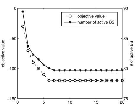
Figure 1: Objective value and number of active base stations as a function of the number of iterations (for one realization). The dashed curve shows the objective in (11). The solid line shows the corresponding number of active base stations for the result of each iteration.

For a fixed user arrival rate leading to a mean number of 400 users in the network, we have observed that, after six iterations, the objective value (11) improves only marginally. In addition to the objective value, we also plot in Fig. 1 the cardinality of the set of active base stations obtained at each iteration. It can be seen that it follows the same trend.

Curves for other user arrival rates have shown a similar pattern. We have always observed a high decreasing rate of the objective value within approximately the first ten iterations and only a marginal decrease afterwards. More iterations have not improved the solution significantly in our scenario.

In Fig. 2 we compare the proposed algorithm with the centralized cell zooming approach in [5]. The results are averaged over ten realizations for the same user arrival rate.

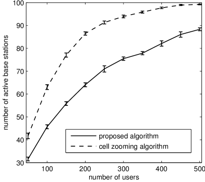
Figure 2: Cardinality of active base station set for different user arrival rates $\lambda$ needed to provide QoS to all users. The results are averaged over ten realizations for each user arrival rate and the height of the error bars shows the estimated error of the mean. The solid line shows our algorithm and the dashed line the cell zooming algorithm from [5]

The simulations show that the number of base stations increases as the user arrival rate increases. It can be observed that, compared with the cell zooming algorithm, our algorithm gives solutions that satisfy the user constraints and use fewer base stations. In addition, the proposed method has other major advantages over the cell zooming approach:

• It can be extended to heterogeneous networks, where we have different power consumption for different network elements.

• It can model the power consumption of the dynamic load, provided that it can be modeled as a concave or convex function.

• It has a strong analytical justification for its good performance.

V Conclusions

In this paper we have developed a novel approach to save energy in wireless networks by selecting a small number of active base stations that guarantees that the QoS (i.e., the minimum data rate) of all users is satisfied. We have shown that recent techniques that have been applied in, for example, compressed sensing can also be successfully applied in this application domain. In particular, the proposed algorithm needs to solve a simple LP at each iteration, so it can easily handle large-scale problems. Simulations show that good sparse solutions are obtained with few iterations. We have also shown that our technique can outperform recent methods such as the cell-zooming approach [5] in practical scenarios. Finally, in stark contrast with the work in [5], the proposed algorithm has other additional advantages such as a good analytical justification and the ability to consider heterogeneous networks and to consider the dynamic transmission power of base stations.

References

- [1] D. Willkomm, S. Machiraju, J. Bolot, and A. Wolisz, “Primary user behavior in cellular networks and implications for dynamic spectrum access,” IEEE Commun. Mag., vol. 47, no. 3, pp. 88 –95, march 2009.
- [2] A. Corliano and M. Hufschmid, “Energieverbrauch der mobilen Kommunikation - Schlussbericht,” Bundesamt für Energie, Schweizerische Eidgenossenschaft, Bern, Swiss, Tech. Rep., February 2008, (in German).
- [3] C. Han, T. Harrold, S. Armour, I. Krikidis, S. Videv, P. Grant, H. Haas, J. Thompson, I. Ku, C.-X. Wang, T. A. Le, M. Nakhai, J. Zhang, and L. Hanzo, “Green radio: radio techniques to enable energy-efficient wireless networks,” IEEE Commun. Mag., vol. 49, no. 6, pp. 46 –54, june 2011.
- [4] P. Gonzalez-Brevis, J. Gondzio, Y. Fan, H. Poor, J. Thompson, I. Krikidis, and P.-J. Chung, “Base station location optimization for minimal energy consumption in wireless networks,” in Vehicular Technology Conference (VTC Spring), 2011 IEEE 73rd, may 2011, pp. 1 –5.
- [5] Z. Niu, Y. Wu, J. Gong, and Z. Yang, “Cell zooming for cost-efficient green cellular networks,” IEEE Commun. Mag., vol. 48, no. 11, pp. 74 –79, november 2010.
- [6] K. Majewski and M. Koonert, “Conservative cell load approximation for radio networks with shannon channels and its application to LTE network planning,” in Telecommunications (AICT), 2010 Sixth Advanced International Conference on, may 2010, pp. 219 –225.
- [7] S. Joshi and S. Boyd, “Sensor selection via convex optimization,” IEEE Trans. Signal Processing, vol. 57, no. 2, pp. 451–462, Feb. 2009.
- [8] E. J. Candes, M. B. Wakin, and S. P. Boyd, “Enhancing sparsity by reweighted minimization,” J. Fourier Anal. Appl., vol. 14, no. 5, pp. 877–905, Dec. 2008.
- [9] I. Yamada, M. Yukawa, and M. Yamagishi, Minimizing the Moreau envelope of nonsmooth convex functions over the fixed point set of certain quasi-nonexpansive mappings, IN: Fixed-Point Algorithms for Inverse Problems in Science and Engineering, H. Bauschke, R. Burachick, P. L. Combettes, V. Elser, D. R. Luke, and H. Wolkowicz, Eds. Springer-Verlag, 2011.
- [10] B. K. Sriperumbudur, D. A. Torres, and G. R. G. Lackriet, “A majorization-minimization approach to the sparse generalized eigenvalue problem,” Machine Learning, vol. 85, no. 1-2, pp. 3–39, Oct. 2011.
- [11] D. R. Hunter and K. Lange, “A tutorial on MM algorithms,” The American Statistician, vol. 58, no. 1, pp. 30–37, Feb. 2004.
- [12] 3GPP, “Further advancements for EUTRA: Physical layer aspects (release 9), TR 36.814 v2.0.1,” http://www.3gpp.org, March 2010.