What is the dimension of a smooth family of complex Hadamard matrices including the Fourier matrix? We address this problem with a power series expansion. Studying all dimensions up to 100 we find that the first order result is misleading unless the dimension is 6, or a power of a prime. In general the answer depends critically on the prime number decomposition of the dimension. Our results suggest that a general theory is possible. We discuss the case of dimension 12 in detail, and argue that the solution consists of two 13-dimensional families intersecting in a previously known 9-dimensional family. A precise conjecture for all dimensions equal to a prime times another prime squared is formulated.

1. Introduction

A type of mathematical problem that arises very often is that one has a set of $M$ algebraic equations in $N$ variables,

$$f_{m}(x_{1},\dots,x_{N})=0\ ,\hskip 22.76219ptm=1,\dots,M\ .$$ (1)

One solution is known, and one asks whether this is an isolated solution, and if not one asks for the dimension of the solution space around that special solution. The problem to be discussed here is of that type, and our aim is to perform a perturbative expansion around the special solution, in order to learn something about the possible answers to the above questions. We will outline a systematic and completely general method to do so.

The particular problem that we will study concerns complex Hadamard matrices. By definition a complex Hadamard matrix is a unitary $N\times N$ matrix all of whose entries have the same modulus. The classification of such matrices has a long history [1]. It has been completed for $N\leq 5$ [2], and much partial information is available in higher dimensions [3, 4, 5]. This classification problem is of interest for many reasons. In quantum theory it is equivalent to the problem of classifying all complementary pairs of bases [6]—now known as Mutually Unbiased Bases [7]—and it can be used to give quantitative content to Bohr’s principle of complementarity [8]. It also forms part of the problem of classifying unitary operator bases [9], which is of importance in quantum information theory, and it arises in operator algebra [10], quantum groups [11], and elsewhere.

A complex Hadamard matrix that exists for any $N$ is the Fourier matrix, whose entries are

$$F_{ij}=\frac{\omega^{ij}}{\sqrt{N}}\ ,\hskip 22.76219pt0\leq i,j\leq N-1\ ,\hskip 22.76219pt\omega=e^{\frac{2\pi i}{N}}\ .$$ (2)

This is the special solution that we are going to expand around. Although we will proceed somewhat differently, in principle one can proceed with this problem by modifying all the matrix elements according to

$$\omega^{ij}\rightarrow\omega^{ij}e^{i\tau_{ij}}\ ,$$ (3)

expanding the phase factors in powers of $\tau_{ij}$, and then solving the unitarity equations order by order in $\tau_{ij}$. To first order in the perturbation this has been done by Tadej and Życzkowski [12], who found that the number of free parameters that survive to first order is

$$D_{1}=\sum_{n=0}^{N-1}\mbox{gcd}(n,N)\ ,$$ (4)

where gcd denotes the greatest common divisor. If $N$ is prime this means that the number of free parameters is $2N-1$. This is the number one would naively expect by counting the number of equations and the number of parameters in the matrix. However, for non-prime values of $N$ the number $D_{1}$ is larger than that.

We can multiply the rows and columns of a complex Hadamard matrix with $2N-1$ overall phase factors, while still preserving the Hadamard property. Hence $2N-1$ parameters are trivial, and it is customary to remove them by presenting complex Hadamard matrices in dephased form, such that the first row and the first column have real and positive entries. The number

$$d_{1}=D_{1}-(2N-1)=\sum_{n=1}^{N-1}(\mbox{gcd}(n,N)-1)$$ (5)

has been called the defect of the Fourier matrix [3], and gives an upper bound on the dimension of any smooth family of dephased complex Hadamard matrices passing through the Fourier matrix. Here we shall call it the linear defect since we found a way of defining order by order a number that is a natural generalization to higher orders of the defect and that coincides with it to first order; we shall then speak of the nth order defect. If $N=p^{k}$ is a prime power the situation is very satisfactory since explicit solutions for dephased Hadamard matrices with $d_{1}$ free parameters are known. These solutions are of an especially simple kind, known as affine families [3]. We are concerned with other values of $N$, for which very little is known. An exception is the special case $N=6$, for which $d_{1}=4$, a 3-dimensional family has been constructed explicitly [13], and a 4-dimensional family has been shown to exist [14, 5]. What is missing so far is a proof that the 4-dimensional family includes the Fourier matrix, and that it is smooth there. Numerical arguments for the truth of this have been presented [15], and we will confirm this conclusion in a perturbative expansion that we carried to order 100.

But it appears that the first order result is misleading in all other cases. Indeed for all values of $N$ less than 101 and not equal to 6 or to a prime power, we will prove that the dimension of the largest smooth family is strictly less than the linear defect.

What we really want to know is by how much the dimension of the solution space differs from $d_{1}$. For $N=12$, which is of some special interest [3], we find that the largest smooth family has dimension 13, while the linear defect is 17 and the largest explicitly known families have dimension 9. The solution in fact consists of two 13-dimensional families intersecting in a 9-dimensional affine family. Our evidence suggests that the situation is similar whenever $N$ is a product of three primes, two of them equal, and we are able to formulate an appealing conjecture of what the final picture is likely to be in this case.

While these results fall short of providing a general solution to our problem they do make us feel that a general solution of a reasonably simple sort does exist.

Most of the paper is devoted to explaining the procedure that leads to the results we have. In section 2 we give a bird’s eyes view of the general method. A linear system of equations has to be solved at each order of the expansion, but the problem is non-trivial because it can happen that a solution exists only if non-linear consistency conditions are imposed on the lower order solutions. In section 3 we begin our discussion of complex Hadamard matrices, and set up the equations that are to be solved perturbatively. In sections 4, 5, and 6 we describe how the general method applies to the problem at hand. In section 7 we investigate all $N\leq 100$, and find out when the dimension of any smooth family is indeed less than $d_{1}$. In section 8 we discuss the case of $N=12$ in full detail, and in section 9 we discuss the cases $N=18,20$, ending with a conjecture for all $N=p_{1}p_{2}^{2}$, where $p_{1},p_{2}$ are prime numbers.

The calculations were partly numerical, partly symbolical, and were performed using Mathematica. We warn the reader at the outset that our results rely on a considerable amount of calculational detail. Depending on interests the reader may therefore want to just glance at section 2—and perhaps at the toy model in Appendix D—and then go directly to section 10 where our conclusions are summarised (and where we offer some speculations concerning the final picture).

In Appendix A we give some background information concerning complex Hadamard matrices, we define the notion of affine families, and we prove some results concerning them that we need in the main text. Appendix B gives an explicit construction of affine families for $N$ equal to a prime power. Appendix C contains an exact second order calculation, valid for all $N$.

For ease of expression we refer to complex Hadamard matrices simply as “Hadamard matrices” from now on, and when we talk of “the dimension of the solution space” we refer to the dimension of the set of dephased Hadamard matrices connected to the Fourier matrix.

2. The method

Let us return to eqs. (1). It is assumed that we know one solution for the $N$ variables. By shifting the variables if necessary, we can arrange that $x_{n}=0$ is a solution of the equations. When we expand the system around this solution the equations take the form

$$f_{m}=A_{m;n}x_{n}+A_{m;n_{1}n_{2}}x_{n_{1}}x_{n_{2}}+...=0\ .$$ (6)

Summation over repeated indices is understood. Assume that the solution $x_{n}=0$ belongs to a family of solutions $x_{n}(\tau_{1},\dots,\tau_{D})$ with $D$ unknown parameters. If the variables are expanded in these parameters we will obtain an expansion of the form

$$x_{n}=x^{(1)}_{n}+x^{(2)}_{n}+x^{(3)}_{n}+...\ .$$ (7)

We do not explicitly write out the dependence on the parameters. Inserting this into eqs. (6) we obtain

$$f_{m}=A_{m;n}x^{(1)}_{n}+A_{m;n}x^{(2)}_{n}+A_{m;n_{1}n_{2}}x^{(1)}_{n_{1}}x^{(1)}_{n_{2}}+...=0\ .$$ (8)

This equation is now to be solved order by order in the hidden parameters. Thus we obtain

$$A_{m;n}x_{n}^{(1)}=0\hskip 256.0748pt$$ (9)

$$A_{m;n}x_{n}^{(2)}=-A_{m;n_{1}n_{2}}x_{n_{1}}^{(1)}x_{n_{2}}^{(1)}\hskip 179.25235pt$$ (10)

$$A_{m;n}x_{n}^{(3)}=-A_{m;n_{1}n_{2}}(x^{(2)}_{n_{1}}x^{(1)}_{n_{2}}+x^{(1)}_{n_{1}}x^{(2)}_{n_{2}})-A_{m;n_{1}n_{2}n_{3}}x^{(1)}_{n_{1}}x^{(1)}_{n_{2}}x^{(1)}_{n_{3}}\hskip 5.69054pt$$ (11)

$$A_{m;n}x^{(4)}_{n}=-A_{m;n_{1}n_{2}}(x^{(3)}_{n_{1}}x^{(1)}_{n_{2}}+x^{(1)}_{n_{1}}x^{(3)}_{n_{2}}+x_{n_{1}}^{(2)}x_{n_{2}}^{(2)})\hskip 71.13188pt$$

$$-A_{m;n_{1}n_{2}n_{3}}(x_{n_{1}}^{(2)}x_{n_{2}}^{(1)}x_{n_{3}}^{(1)}+x_{n_{1}}^{(1)}x_{n_{2}}^{(2)}x_{n_{3}}^{(1)}+x_{n_{1}}^{(1)}x_{n_{2}}^{(1)}x_{n_{3}}^{(2)})\hskip 8.53581pt$$ (12)

$$-A_{m;n_{1}n_{2}n_{3}n_{4}}x_{n_{1}}^{(1)}x_{n_{2}}^{(1)}x_{n_{3}}^{(1)}x_{n_{4}}^{(1)}\ ,\hskip 122.34685pt$$

and so on to higher orders. At each order then we are faced with a linear system; homogeneous to first order and heterogeneous to the higher orders. At each order higher than the first this linear system may or may not—depending on the form of the original equations—impose restrictions on the solutions obtained in lower orders.

To deal with these linear systems we introduce a pseudo-inverse of the $M\times N$ matrix $A_{m;n}$. This is a matrix $\hat{A}$ obeying $A\hat{A}A=A$. For this general discussion it is natural to choose the Moore-Penrose inverse for this purpose, since—due to some extra conditions—it is uniquely defined and easily computed [16]. The relevant theorem is that the linear system

$$AX=B$$ (13)

admits a solution if and only if

$$({\bf 1}-A\hat{A})B=0\ .$$ (14)

When this consistency condition is obeyed the general solution is

$$X=\hat{A}B+({\bf 1}-\hat{A}A)Z\ ,$$ (15)

where the $N$ components of the column vector $Z$ are arbitrary. The matrix ${\bf 1}-\hat{A}A$ typically has rank less than $N$, so the number of free parameters in the homogeneous solution is typically less than $N$.

The first order equations are homogeneous, and admit the homogeneous solution

$$x_{n}^{(1)}=(\delta_{nn_{1}}-\hat{A}_{n;m}A_{m;n_{1}})z^{(1)}_{n_{1}}\equiv h_{n}^{(1)}\ .$$ (16)

The number of free parameters in the solution gives an upper bound on the dimension of the solution space. To second order the solution is a sum of a homogeneous and a heterogeneous part,

$$x_{n}^{(2)}=h_{n}^{(2)}-\hat{A}_{n;m}A_{m;n_{1}n_{2}}h_{n_{1}}^{(1)}h_{n_{2}}^{(1)}\ ,$$ (17)

provided that the consistency condition

$$(\delta_{mm_{1}}-A_{m;n}\hat{A}_{n;m_{1}})A_{m_{1};n_{1}n_{2}}h_{n_{1}}^{(1)}h_{n_{2}}^{(1)}=0$$ (18)

holds. Assume for the sake of the argument that it does, and write the solution as

$$x_{n}^{(2)}=h_{n}^{(2)}+H_{n}^{(2)}\ ,$$ (19)

where the heterogeneous part is a known second order polynomial in $h_{n}^{(1)}$ (obeying $h_{n}^{(1)}\rightarrow\lambda h_{n}^{(1)}\Rightarrow H_{n}^{(2)}\rightarrow\lambda^{2}H_{n}^{(2)}$). To third order the heterogeneous part of the solution is

$$H_{n}^{(3)}=-\hat{A}_{n;m}A_{m;n_{1}n_{2}}(x^{(2)}_{n_{1}}x^{(1)}_{n_{2}}+x_{n_{1}}^{(1)}x_{n_{2}}^{(2)})-\hat{A}_{n;m}A_{m;n_{1}n_{2}n_{3}}x^{(1)}_{n_{1}}x_{n_{2}}^{(1)}x_{n_{3}}^{(1)}\ ,$$ (20)

provided that

$$({\bf 1}-A\hat{A})_{m,m_{1}}A_{m_{1};n_{1}n_{2}}(x^{(2)}_{n_{1}}x^{(1)}_{n_{2}}+x_{n_{1}}^{(1)}x_{n_{2}}^{(2)})+$$

(21)

$$+({\bf 1}-A\hat{A})_{m,m_{1}}A_{m_{1};n_{1}n_{2}n_{3}}x^{(1)}_{n_{1}}x^{(1)}_{n_{2}}x_{n_{3}}^{(1)}=0\ .$$

Due to the symmetrisation, and the second order consistency condition, this condition can be written as

$$({\bf 1}-A\hat{A})_{m,m_{1}}\left(A_{m_{1};n_{1}n_{2}}(H^{(2)}_{n_{1}}h^{(1)}_{n_{2}}+h_{n_{1}}^{(1)}H_{n_{2}}^{(2)})+A_{m_{1};n_{1}n_{2}n_{3}}h^{(1)}_{n_{1}}h^{(1)}_{n_{2}}h_{n_{3}}^{(1)}\right)=0\ .$$ (22)

This is a third order polynomial in $h_{n}^{(1)}$. As long as the consistency conditions continue to hold to order $s-1$, the consistency condition at order $s$ will always be a set of polynomial equations of order $s$ in $h_{n}^{(1)}$. If they hold to all orders the homogeneous solutions of order higher than one can be set to zero by means of a redefinition of the first order solution, and we are done.

Assume for the sake of the argument that the consistency conditions do break down at third order. Then one must solve a set of third order polynomial equations that will restrict the first order homogeneous solution. We cannot say by how much the upper bound on the dimension of the solution space drops until these equations have been solved.

When we continue to the next order we can still write

$$x_{n}^{(4)}=h_{n}^{(4)}+H_{n}^{(4)}\ ,$$ (23)

where the heterogeneous part is a polynomial of fourth order in the parameters and depending on $h_{n}^{(1)}$, $h_{n}^{(2)}$, and $h_{n}^{(3)}$. The consistency condition at fourth order is

$$({\bf 1}-A\hat{A})_{mm_{1}}\big{(}A_{m_{1};n_{1}n_{2}}(H^{(3)}_{n_{1}}h^{(1)}_{n_{2}}+h^{(1)}_{n_{1}}H^{(3)}_{n_{2}}+\hskip 85.35826pt$$

$$+h^{(2)}_{n_{1}}H^{(2)}_{n_{2}}+H^{(2)}_{n_{1}}h^{(2)}_{n_{2}}+H^{(2)}_{n_{1}}H^{(2)}_{n_{2}})+\hskip 42.67912pt$$

$$+A_{m_{1};n_{1}n_{2}n_{3}}(h^{(2)}_{n_{1}}h^{(1)}_{n_{2}}h^{(1)}_{n_{3}}+h^{(1)}_{n_{1}}h^{(2)}_{n_{2}}h^{(1)}_{n_{3}}+h^{(1)}_{n_{1}}h^{(1)}_{n_{2}}h^{(2)}_{n_{3}}+$$

(24)

$$+H^{(2)}_{n_{1}}h^{(1)}_{n_{2}}h^{(1)}_{n_{3}}+h^{(1)}_{n_{1}}H^{(2)}_{n_{2}}h^{(1)}_{n_{3}}+h^{(1)}_{n_{1}}h^{(1)}_{n_{2}}H^{(2)}_{n_{3}})\hskip 14.22636pt$$

$$+A_{m_{1};n_{1}n_{2}n_{3}n_{4}}h^{(1)}_{n_{1}}h^{(1)}_{n_{2}}h^{(1)}_{n_{3}}h^{(1)}_{n_{4}}\big{)}=0\ .\hskip 42.67912pt$$

Note that $h^{(3)}_{n}$ does not appear because the consistency condition is fullfilled at order two. This is a set of linear equations for the $h^{(2)}_{n}$, briefly $Uh^{(2)}_{n}=V$. The solution will be a quotient of two polynomials in $h^{(1)}_{n}$ which is homogeneous of order two in that variable. If the rank of the matrix $U$ is equal to the number $u$ of variables $h^{(1)}_{n}$ fixed by the third order consistency equations then the corresponding variables are fixed once and for all (it is easy to check that to fifth order one gets consistency equations of the type $Uh^{(3)}_{n}=W$, where $U$ is the same matrix). However these linear systems come with their own consistency conditions which, if not automatically satisfied, will further fix the $h^{(1)}_{n}$ and further lower the defect.

We have not investigated in any systematic manner what happens if these higher order consistency conditions break down at some higher order–although this does happen in some of the concrete cases that we study below. If the rank of $U$ is lower than $u$ then the remaining $h^{(2)}_{n}$ must be fixed at higher order by non-linear equations (as would be the case for systems having sets of solutions which are tangent at the point around which we are expanding). This did not happen in the particular cases under study; also the toy model in Appendix D provides a reassuring consistency check.

It is time to turn to the subject we want to deal with. We will then be able to adapt our method to the special form of the equations we encounter. In particular the Moore-Penrose inverse will not be needed.

3. The Hadamard equations

The equations ensuring that a matrix is a Hadamard matrix define an algebraic variety of some sort [18]. Since our aim is to solve these equations order by order in an expansion around the Fourier matrix $F$ we begin by performing a discrete Fourier transformation of all our matrices, that is

$$H\rightarrow M=HF^{\dagger}\ ,$$ (25)

where the dagger denotes hermitian conjugation. This means that the Fourier matrix itself is represented by the unit matrix. We prefer to represent the Fourier matrix with the zero matrix, so we shift the matrix to

$$X={\bf 1}-M\ .$$ (26)

We must now formulate the condition that $H$ be a Hadamard matrix as a set of equations for the matrix $X$. In order to be able to address the equations in an efficient way we aim for a subset of equations in which the complex conjugates of the matrix elements do not occur.

For this purpose we introduce the permutation matrix $P$ with matrix elements

$$P_{ij}=\delta_{i+1,j}\ .$$ (27)

This matrix generates the cyclic group of order $N$, and has the columns of the Fourier matrix as its eigenvectors. We denote the commutator of two matrices by $[A,B]$, and the vector of diagonal elements of a matrix by diag$(A)$.

Theorem 1: $H$ is a Hadamard matrix if and only if $M=HF^{\dagger}$ obeys

$$MM^{\dagger}={\bf 1}$$ (28)

$$\mbox{diag}(MP^{n}M^{\dagger})=0\ ,\hskip 22.76219ptn\neq 0\ \mbox{mod}\ N\ ,$$ (29)

where $P$ is the permutation matrix defined above. For the matrix $X={\bf 1}-M$ these equations read

$$X+X^{\dagger}=XX^{\dagger}$$ (30)

$$\mbox{diag}\left(\sum_{p=0}^{\infty}[P^{n},X]X^{p}\right)=0\ ,\hskip 22.76219ptn\neq 0\ \mbox{mod}\ N\ ,$$ (31)

at least in a neighbourhood of the Fourier matrix.

Proof: Direct calculation shows that

$$(MP^{n}M^{\dagger})_{ii}=\sum_{j}\omega^{nj}|H_{ij}|^{2}\ ,$$ (32)

and elementary properties of the discrete Fourier transform now establish that eq. (29) is necessary and sufficient, given that $M$ is unitary. Since unitarity is imposed separately we may replace the matrix $M^{\dagger}$ by the matrix $M^{-1}$ in eq. (29). Expanding $M^{-1}=({\bf 1}-X)^{-1}$ in a geometric series and using the property that

$$\mbox{diag}\left(P^{n}\sum_{p=0}^{\infty}X^{p}\right)=\mbox{diag}\left(P^{n}\sum_{p=0}^{\infty}X^{p+1}\right)$$ (33)

we arrive at eq. (31). The unitarity condition on $M$ is clearly equivalent to eq. (30). $\Box$

The plan now is to first solve eq. (31) order by order in a perturbative expansion, using complex entries with no complex conjugates appearing, and to impose the unitarity condition at the end. The alternative, to impose unitarity at each order from the beginning, is less convenient for symbolic calculations using Mathematica.

To deal with eq. (31) following the method outlined in section 2 the first step is to expand $X$ order by order in the unknown parameters. To follow the letter of the method we should reshape the matrix $X$ into a vector, but we will not actually do so since it will turn out that we can solve directly for the matrix $X$.

Thus we write

$$X=\sum_{s=1}^{\infty}X^{(s)}\ .$$ (34)

Inserting this into eq. (31), which itself contains an infinite sum to be expanded, we find that the equations at each order $s$ form the inhomogeneous linear system

$$\mbox{diag}\left([P^{n},X^{(s)}]+B^{(s,n)}\right)=0\ ,$$ (35)

where $B^{(s,n)}$ can be computed in terms of quantities determined at lower orders. The first few orders are

$$\mbox{diag}\left([P^{n},X^{(1)}]\right)=0\hskip 233.31259pt$$ (36)

$$\mbox{diag}\left([P^{n},X^{(2)}]+[P^{n},X^{(1)}]X^{(1)}\right)=0\hskip 153.64487pt$$ (37)

$$\mbox{diag}\left([P^{n},X^{(3)}]+[P^{n},X^{(2)}]X^{(1)}+[P^{n},X^{(1)}](X^{(2)}+X^{(1)}X^{(1)})\right)=0\ .$$ (38)

At each order $s$ this is a linear inhomogeneous equation in the unknown $X^{(s)}$. We record that

$$B^{(s,n)}=\sum_{p=1}^{s-1}\sum_{\begin{subarray}{c}s_{i}\geq 1\\ s_{0}+\dots+s_{p}=s\end{subarray}}[P^{n},X^{(s_{0})}]X^{(s_{1})}\dots X^{(s_{p})}\ .$$ (39)

We will need this result in the proofs of Theorems 4 and 5 below.

We end this section with two comments. The first concerns transposition of Hadamard matrices: If $H$ is a Hadamard matrix so is its transpose $H^{\rm T}$, a fact that will play a role when we discuss explicit solutions later on. It is easy to show that

$$H\rightarrow H^{\rm T}\hskip 14.22636pt\Leftrightarrow\hskip 14.22636ptX\rightarrow FX^{\rm T}F^{\dagger}\ .$$ (40)

Hence transposition is slightly obscured by the discrete Fourier transform.

The second comment concerns dephasing: In the introduction we observed that any Hadamard matrix admits $2N-1$ free parameters that are in a sense trivial, and that these trivial parameters can be removed by insisting that the first row and the first column of the matrix has entries equal to $1/\sqrt{N}$ only. If we dephase the first row of the matrix $H$ we will obtain a matrix $X$ whose first row contains zero entries only. If we also dephase the first column of $H$ we find that $X$ takes the form

$$X=\left[\begin{array}[]{cccc}0&0&\dots&0\\ 0&&&\\ \vdots&&\tilde{X}&\\ 0&&&\end{array}\right]\ ,\hskip 34.1433pt\sum_{j=1}^{N-1}\tilde{X}_{ij}=0\ .$$ (41)

In our calculations we did not impose this condition, but we will state our results in terms of the dimension of the set of dephased matrices.

4. The homogeneous system

We begin by solving the linear first order system ($n\neq 0$ mod $N$)

$$\mbox{diag}[P^{n},X^{(1)}]=0\hskip 14.22636pt\Leftrightarrow\hskip 14.22636ptX^{(1)}_{i+n,i}-X^{(1)}_{i,i-n}=0\ .$$ (42)

We observe that there is no condition on the diagonal elements of $X$, and that the equalities that do arise connect only elements on some given displaced diagonal. On the $n$th displaced diagonal we obtain the string of equalities

$$X_{i,i-n}=X_{i+n,i}=X_{i+2n,i+n}=...\ .$$ (43)

It pays to think of the matrix as built up from displaced diagonals rather than columns, so we introduce the parametrisation

$$X_{i,j}=x_{i,j-i}\ .$$ (44)

Recall that all matrix indices obey modulo $N$ arithmetic. Our string of equalities becomes

$$x_{i,-n}=x_{i+n,-n}=x_{i+2n,-n}=...\ .$$ (45)

Now let the greatest common divisor of $n$ and $N$ be denoted by $g$, so that

$$N=gr\ ,\hskip 22.76219ptn=gs\ .$$ (46)

Taking the modulo $N$ arithmetic into account we see that the string of equalities ends with an identity after $r$ steps,

$$x_{i,-n}=...=x_{i+rn,-n}\equiv x_{i+sN,-n}\equiv x_{i,-n}\ .$$ (47)

There are $r-1$ non-trivial equalities here. Written in a more transparent fashion they are

$$x_{i,-n}=x_{i+g,-n}=x_{i+2g,-n}=...=x_{i+(r-1)g,-n}\ .$$ (48)

See Fig. 1. This means that the $n$th displaced diagonal consists of $g$ sets of $r$ identical elements. Recalling that the elements on the main diagonal are unrestricted it follows that the number of free parameters at first order is

$$\sum_{n=0}^{N-1}\mbox{gcd}(n,N)=N+\sum_{n=1}^{N-1}\mbox{gcd}(n,N)\ .$$ (49)

This agrees with the result (4) due to Tadej and Życzkowski [12], except that at this stage our parameters are complex since we have not yet imposed condition (30). To linear order condition (30) evidently means that we end up with exactly this number of real parameters, so the agreement is in fact complete. If $N=p$ is a prime number all elements on each displaced diagonal are set equal. In this case then there are exactly $2N-1$ free parameters in the solution, $N$ of them coming from the unrestricted main diagonal, which means that the dephased Fourier matrix is isolated, not belonging to a continuous family of dephased Hadamard matrices.

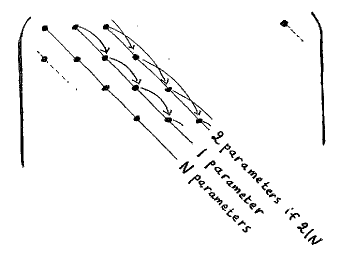
Figure 1: The proof of theorem 2; one should think of a matrix in terms of its diagonals, not in terms of its rows or columns.

In effect we have proved

Theorem 2: At any order, the homogeneous solution to our linear system can be written as

$$X^{(s)}_{i,j}=x^{(s)}_{i\ {\rm mod\ gcd}(j-i,N),j-i\ {\rm mod}\ N}\ .$$ (50)

An illustration of the proof is given in Fig. 1. If $N=p$ is a prime number $X$ is a circulant matrix, except that its main diagonal is unrestricted. Its dephased form is zero. A more interesting example is that of $N=6$, for which the first order solution is

$$X^{(1)}=\left(\begin{array}[]{cccccc}x_{0,0}&x_{0,1}&x_{0,2}&x_{0,3}&x_{0,4}&x_{0,5}\\ x_{0,5}&x_{1,0}&x_{0,1}&x_{1,2}&x_{1,3}&x_{1,4}\\ x_{0,4}&x_{0,5}&x_{2,0}&x_{0,1}&x_{0,2}&x_{2,3}\\ x_{0,3}&x_{1,4}&x_{0,5}&x_{3,0}&x_{0,1}&x_{1,2}\\ x_{0,2}&x_{1,3}&x_{0,4}&x_{0,5}&x_{4,0}&x_{0,1}\\ x_{0,1}&x_{1,2}&x_{2,3}&x_{1,4}&x_{0,5}&x_{5,0}\end{array}\right)\ .$$ (51)

When we remove the trivial parameters by dephasing the Hadamard matrix this is

$$X^{(1)}=\left(\begin{array}[]{cccccc}0&0&0&0&0&0\\ 0&d_{1}&0&x_{1,2}&x_{1,3}&x_{1,4}\\ 0&0&d_{2}&0&0&x_{2,3}\\ 0&x_{1,4}&0&d_{3}&0&x_{1,2}\\ 0&x_{1,3}&0&0&d_{4}&0\\ 0&x_{1,2}&x_{2,3}&x_{1,4}&0&d_{5}\end{array}\right)\ .$$ (52)

Now the diagonal elements $d_{i}$ are dependent parameters since dephasing the Hadamard matrix means that the column sums of $X$ vanish, so the number of free parameters equals $4$. The affine Fourier family (see Appendix A) is obtained by setting $x_{1,3}=x_{2,3}=0$, and its transpose by setting $x_{1,2}=x_{1,4}=0$; to see what eq. (40) implies for $X$ when $H$ is transposed it is helpful to begin with the observation that circulant matrices are diagonalised by the Fourier matrix.

5. The heterogeneous systems

The question now is whether there are non-trivial consistency conditions on the linear systems that appear when we insert the expansion (34) in eq. (31). If so the first order result is misleading, and the true dimension of the solution space is lower than the linear result suggests it should be. If $N$ is a prime or a power of a prime we know—see section 1—that this cannot happen, but for all other choices of $N$ we move on unknown ground.

The equations that we are faced with take the form (35). Our aim is to bring their solution to a form precise enough to enable us to implement it in Mathematica. This is achieved in the following two theorems.

Theorem 3: The general solution to the heterogeneous linear system (35) is

$$X^{(s)}_{i,j}=x^{(s)}_{i\ {\rm mod}\ {\rm gcd}(j-i,N),j-i}+\sum_{q=0}^{m[i,j,N]-1}B^{(s,i-j)}_{i+q(i-j),i+q(i-j)}\ ,$$ (53)

subject to the consistency conditions

$$\sum_{q=0}^{N/{\rm gcd}(n,N)-1}B^{(s,n)}_{i+q\ {\rm gcd}(n,N),i+q\ {\rm gcd}(n,N)}=0\ ,$$ (54)

where $n\in\{1,\dots,N-1\}$, $i\in\{0,\dots,\mbox{gcd}(n,N)-1\}$ in the consistency conditions, and the $x_{i,j-i}$ are free parameters. The integer $m=m[i,j,N]$ is given by

$$m=\frac{i\ \mbox{mod gcd}(i-j,N)-i}{\mbox{gcd}(i-j,N)}\left(\frac{i-j}{\mbox{gcd}(i-j,N)}\right)^{-1}\ \mbox{mod}\ \frac{N}{\mbox{gcd}(i-j,N)}\ ,$$ (55)

where the inverse is the multiplicative inverse modulo $N/\mbox{gcd}(i-j,N)$.

In words, the consistency conditions at order $s$ say that for each displaced diagonal labelled by $n$ the $B^{(s,n)}$ sum to zero when summed over a set of positions with equal values of the parameters in the homogeneous solution.

Proof: Using explicit matrix indices, always taken modulo $N$, eq. (35) becomes

$$X^{(s)}_{i,i-n}=X^{(s)}_{i+n,i}+B^{(s,n)}_{ii}\ .$$ (56)

Setting $n=i-j$ we find by iterating in $m$ steps that

$$X^{(s)}_{i,j}=X^{(s)}_{i+m(i-j),j+m(i-j)}+\sum_{q=0}^{m-1}B^{(s,i-j)}_{i+q(i-j),i+q(i-j)}\ .$$ (57)

When

$$m(i-j)=0\ \ \mbox{mod}\ N\hskip 14.22636pt\Leftrightarrow\hskip 14.22636ptm=\frac{kN}{\mbox{gcd}(i-j,N)}\ ,\ \ k\in{\bf Z}$$ (58)

we obtain a consistency condition which—after a slight reordering of the sum—is exactly eq. (54). This is the same reordering that was used to go from (47) to (48).

Now we must find a particular solution of the heterogeneous system. We begin by choosing all matrix elements corresponding to independent parameters in the homogeneous solution to zero, beginning with all elements in the upmost row and continuing downwards until the independent elements are exhausted. For this particular solution

$$i\mbox{\ mod gcd}(i-j,N)=i\hskip 14.22636pt\Rightarrow\hskip 14.22636ptX^{(s)}_{i,j}=0\ .$$ (59)

Coming back to eq. (57), which relates elements along the $(i-j)$th diagonal in steps of gcd$(i-j,N)$, we see that we obtain a particular solution fully determined by the lower order solution provided that the first term on the right hand side vanishes. Given the conditions (59) that we already imposed this will be ensured if we can find (for each $i,j,N$) an integer $m$ such that

$$i+m(i-j)=i+m(i-j)\ \mbox{mod gcd}(i-j,N)=i\ \mbox{mod gcd}(i-j,N)\ .$$ (60)

This is equivalent to

$$\left\{m\frac{i-j}{\mbox{gcd}(i-j,N)}=\frac{i\ \mbox{mod gcd}(i-j,N)-i}{\mbox{gcd}(i-j,N)}\right\}\ \mbox{mod}\frac{N}{\mbox{gcd}(i-j,N)}\ .$$ (61)

The solution in the range $\{0,...,N/\mbox{gcd}(i-j,N)\}$ is given in eq. (55). The modular multiplicative inverse used there exists since the numbers $(i-j)/\mbox{gcd}(i-j,N)$ and $N/\mbox{gcd}(i-j,N)$ are coprime. Using this value of $m$ in eq. (57) gives the particular solution, and we arrive at the general solution (53) by adding the general solution of the homogeneous equations. $\Box$

To illustrate the proof we give the particular solution for $N=6$:

$$\left(\begin{array}[]{cccccc}0&0&0&0&0&0\\ \\ \sum_{0}^{4}B_{1+q}^{(1)}&0&B_{1}^{(5)}&0&0&0\\ \\ \sum_{0}^{1}B_{2+2q}^{(2)}&\sum_{0}^{3}B_{2+q}^{(1)}&0&\sum_{0}^{1}B_{2-q}^{(5)}&B_{2}^{(4)}&0\\ \\ B_{3}^{(3)}&\sum_{0}^{1}B_{3+2q}^{(2)}&\sum_{0}^{2}B_{3+q}^{(1)}&0&\sum_{0}^{2}B_{3-q}^{(5)}&B_{3}^{(4)}\\ \\ \sum_{0}^{1}B_{4-2q}^{(4)}&B_{4}^{(3)}&B_{4}^{(2)}&\sum_{0}^{1}B_{4+4q}^{(1)}&0&\sum_{0}^{3}B_{4-q}^{(5)}\\ \\ \sum_{0}^{4}B_{5-q}^{(5)}&\sum_{0}^{1}B_{5-2q}^{(4)}&B_{5}^{(3)}&B_{5}^{(2)}&B_{5}^{(1)}&0\end{array}\right)$$ (62)

where (for typographical reasons) we let $B^{(s,n)}_{i,i}$ be denoted by $B_{i}^{(n)}$.

To make use of theorem 3 we must compute the inhomogeneous term $B^{(s,n)}_{i,i}$. This is achieved in the next theorem.

Theorem 4: The inhomogeneous part $B^{(s,n)}$ is given iteratively by

$$B^{(1,n)}=0$$ (63)

$$B^{(s,n)}=\sum_{r=1}^{s-1}\left([P^{n},X^{(r)}]+B^{(r,n)}\right)X^{(s-r)}\ .$$ (64)

The proof is straightforward, using expression (39).

It is hard to continue the discussion with any generality, but we have been able to prove that the consistency conditions arising at second order, eqs. (37), are identically satisfied for all $N$. We give a brief sketch of a proof in Appendix C. At third order the consistency conditions do break down for some values of $N$, as will be discussed in section 7.

6. The unitarity equations

We must now impose the unitarity condition (30) on the solutions obtained in section 5. When $X$ is expanded in a power series the unitarity condition at order $s$ reads

$$X^{(s)}+\left(X^{(s)}\right)^{\dagger}=\sum_{r=1}^{s-1}X^{(s-r)}\left(X^{(r)}\right)^{\dagger}\ .$$ (65)

We insert the solution

$$X^{(s)}_{i,j}=x_{i,j-i}^{(s)}+H^{(s)}_{i,j}(X^{(1)},\dots,X^{(s-1)})\ ,$$ (66)

where $H_{i,j}^{(s)}$ is the heterogeneous part as given in theorem 3, and $x^{(s)}_{i,j-i}$ is short for $x^{(s)}_{i\ {\rm mod\ gcd}(j-i,N),j-i\ {\rm mod}\ N}$. The equations to be solved are now

$$x^{(s)}_{i,j-i}+\bar{x}^{(s)}_{i,i-j}=F_{i,j}^{(s)}\ ,$$ (67)

where complex conjugation is denoted by an overbar. We used $i\ {\rm mod\ gcd}(j-i,N)=j\ {\rm mod\ gcd}(j-i,N)$, and we also defined

$$F^{(s)}=\sum_{r=1}^{s-1}X^{(s-r)}\left(X^{(r)}\right)^{\dagger}-H^{(s)}-\left(H^{(s)}\right)^{\dagger}\ .$$ (68)

Note that this depends on the solution only to orders less than $s$.

Theorem 5: The matrix $H=({\bf 1}-X)F$ is unitary order by order in the perturbative expansion provided that the following conditions are imposed on its matrix elements:

$$\mbox{Re}\left[x_{i,0}^{(s)}\right]=\frac{1}{2}F_{i,i}^{(s)}$$ (69)

$$\mbox{Re}\left[x_{i\mbox{{\small\ mod}}\ N/2,N/2}^{(s)}\right]=\frac{1}{2}F_{i,i+N/2}^{(s)}\hskip 14.22636pt\mbox{\sl if}\ N\ \mbox{\sl is even}$$ (70)

$$x^{(s)}_{i\mbox{{\small\ mod gcd}}(n,N),-n}=F_{i,j}^{(s)}-\bar{x}^{(s)}_{i\mbox{{\small\ mod gcd}}(n,N),n}\hskip 14.22636pt\mbox{\sl for}\ 0<n<N/2\ .$$ (71)

Proof: Most of the calculation is already done, but in eqs. (70-71) some equations are repeated as $i$ runs through its $N$ values and we must prove consistency, namely that $F^{(s)}$ solves the same linear system as does the homogeneous solution. Thus we require

$$\mbox{diag}[P^{n},F^{(s)}]=0\ .$$ (72)

Using the fact that diag$\{[P^{n},H^{(s)}]\}=-\mbox{diag}\{B^{(s,n)}\}$ and recalling that $(P^{n})^{\dagger}=P^{-n}$, a calculation shows that

$$\mbox{diag}[P^{n},F^{(s)}]=\mbox{diag}\left(\sum_{r=1}^{s-1}[P^{n},X^{(s-r)}]X^{(r)\dagger}+B^{(s,n)}\right)-\ \ \$$

(73)

$$\hskip 99.58464pt-\mbox{diag}\left(\sum_{r=1}^{s-1}[P^{-n},X^{(s-r)}]X^{(r)\dagger}+B^{(s,-n)}\right)^{\dagger}\ .$$

Next we show directly from eq. (65) that

$$X^{(s)\dagger}=-\sum_{p=1}^{s}\sum_{\begin{subarray}{c}s_{i}\geq 1\\ s_{1}+\dots+s_{p}=s\end{subarray}}X^{(s_{1})}\dots X^{(s_{p})}\ .$$ (74)

Using this result, and using eq. (39) to substitute for $B^{(s,n)}$, we see that the right hand side of eq. (73) vanishes, as was to be shown. $\Box$

We illustrate this by imposing unitarity on the first order result for $N=6$ given in eq. (51). It now reads

$$X^{(1)}=\left(\begin{array}[]{rrrrrr}y_{0,0}&x_{0,1}&x_{0,2}&y_{0,3}&-\bar{x}_{0,2}&-\bar{x}_{0,1}\\ -\bar{x}_{0,1}&y_{1,0}&x_{0,1}&x_{1,2}&y_{1,3}&-\bar{x}_{1,2}\\ -\bar{x}_{0,2}&-\bar{x}_{0,1}&y_{2,0}&x_{0,1}&x_{0,2}&y_{2,3}\\ y_{0,3}&-\bar{x}_{1,2}&-\bar{x}_{0,1}&y_{3,0}&x_{0,1}&x_{1,2}\\ x_{0,2}&y_{1,3}&-\bar{x}_{0,2}&-\bar{x}_{0,1}&y_{4,0}&x_{0,1}\\ x_{0,1}&x_{1,2}&y_{2,3}&-\bar{x}_{1,2}&-\bar{x}_{0,1}&y_{5,0}\end{array}\right)\ .$$ (75)

The matrix elements denoted $y_{i,j}$ are purely imaginary. The others are complex and related in pairs by complex conjugation.

The important point is that the unitarity condition simply cuts the number of free parameters in half; in other words if there were $d$ complex parameters in the perturbative solution of eq. (31) then we end up with $d$ real parameters after imposing unitarity. The difficult consistency conditions appear only in the solution of eq. (31).

We are unable to show in general that unitarity also cuts the number of variables fixed by a non-trivial consistency condition in half. Still, in section 8 we prove that this indeed happens for the particular case of $N=12$. We believe that the issue must be dealt with on a case-by-case basis.

7. When do the consistency conditions break down?

As was mentioned at the end of section 5 the consistency conditions always hold to second order. For third order and higher we have used Mathematica to perform the calculation numerically, using random values for the free parameters. For some dimensions to be discussed below the calculation was also performed symbolically. When $N$ is a power of a prime we found no breakdown in the consistency conditions to the orders we checked. This had to be so because in this case there do exist affine families of Hadamard matrices with their dimension given by the linear defect $d_{1}$. For $N=2\cdot 3=6$ we computed (numerically) the higher order contributions to order 100 in the perturbation series, without encountering any breakdown of the consistency conditions. There seemed to be no point in going further. The calculation clearly supports the extant conjecture that the $N=6$ Fourier matrix belongs to a smooth 4-parameter family of dephased Hadamard matrices.

For all other choices of $N\leq 100$ we found that the consistency conditions do break down at some order $s$, according to a definite pattern. Let $p_{1},p_{2},p_{3},\dots$ be different prime numbers. Then the consistency conditions

• hold to all orders if $N$ is a power of a prime (and to order 100 if $N=6)$

• break at order 11 if $N=10$

• break at order 7 if $N=2p_{1}$ and $p_{1}>5$ is odd

• break at order 5 if $N=p_{1}p_{2}$ is odd

• break at order 4 if $N=p_{1}^{k_{1}}p_{2}^{k_{2}}$ and $k_{1}k_{2}>1$

• break at order 3 if $N=p_{1}^{k_{1}}p_{2}^{k_{2}}p_{3}^{k_{3}}$.

For $N\leq 100$ there are no examples of an integer that is a product of four different primes, but we did check that the consistency conditions break at order 3 for $N=2\cdot 3\cdot 5\cdot 7=210$. Again, Appendix C contains a proof that the consistency conditions always hold to second order.

It is very encouraging that an orderly pattern emerges.

8. The $N=12$ case

What we really want to know is the dimension of the solution space to all orders. We will discuss the case $N=12$ in detail. The defect at linear order is $d_{1}=17$, and it is also known that the Fourier matrix belongs to seven distinct affine families of dimension $d_{A}=9$ [3]. Therefore we know at the outset that the dimension of the dephased solution space lies between these bounds.

When the calculation is continued beyond linear order we find that the consistency conditions for the linear system break down at fourth order in the perturbation, resulting in a set of fourth order polynomials to be solved.

There are 40 variables in the first order solution. 23 of those are trivial (since they determine the $2N-1$ free phases) so we expect the consistency conditions to depend on 17 variables. There are only 13 conditions that do not vanish automatically, and close inspection shows that only 13 linear combinations of the variables enter these equations. To be precise, the consistency conditions are fourth order polynomials in the 13 variables

$$\begin{array}[]{ll}x_{2}=x_{0,2}-x_{1,2}\\ x_{10}=x_{0,10}-x_{1,10}\\ x_{4a}=x_{0,4}-x_{2,4}\\ x_{4b}=x_{1,4}-x_{3,4}\\ x_{8a}=x_{0,8}-x_{2,8}\\ x_{8b}=x_{1,8}-x_{3,8}\\ x_{6a}=x_{0,6}-x_{3,6}\\ x_{6b}=x_{4,6}-x_{1,6}\\ x_{6c}=x_{2,6}-x_{5,6}\end{array}\hskip 28.45274pt\begin{array}[]{ll}x_{3a}=2x_{0,3}-x_{1,3}-x_{2,3}\\ x_{3b}=2x_{1,3}-x_{0,3}-x_{2,3}\\ x_{3c}=2x_{2,3}-x_{0,3}-x_{1,3}\\ x_{9a}=2x_{0,9}-x_{1,9}-x_{2,9}\\ x_{9b}=2x_{1,9}-x_{0,9}-x_{2,9}\\ x_{9c}=2x_{2,9}-x_{0,9}-x_{1,9}&\ .\end{array}$$ (76)

Note that there are only 13 independent variables, because $x_{3a}+x_{3b}+x_{3c}=x_{9a}+x_{9b}+x_{9c}=0$.

We next define the auxiliary polynomials

$$p_{1}=x_{3a}^{2}+x_{9a}^{2}\hskip 22.76219ptp_{2}=x_{3b}^{2}+x_{9b}^{2}\hskip 22.76219ptp_{3}=x_{3c}^{2}+x_{9c}^{2}$$ (77)

$$p_{4}=x_{4a}^{2}-x_{4b}^{2}\hskip 17.07164ptp_{5}=x_{8a}^{2}-x_{8b}^{2}\hskip 17.07164ptp_{6}=x_{4a}x_{8a}-x_{4b}x_{8b}\ .$$ (78)

The complete set of consistency conditions now takes the form

$$p_{1}p_{6}=p_{2}p_{6}=p_{3}p_{6}=0$$ (79)

$$(p_{1}+p_{2}+p_{3})p_{4}=(p_{1}+p_{2}+p_{3})p_{5}=0$$ (80)

$$x_{4a}x_{10}(p_{1}+p_{2}+p_{3})+x_{8a}(x_{6a}p_{1}+x_{6b}p_{2}+x_{6c}p_{3})=0$$ (81)

$$x_{4b}x_{10}(p_{1}+p_{2}+p_{3})+x_{8b}(x_{6a}p_{1}+x_{6b}p_{2}+x_{6c}p_{3})=0$$ (82)

$$x_{8a}x_{2}(p_{1}+p_{2}+p_{3})+x_{4a}(x_{6a}p_{1}+x_{6b}p_{2}+x_{6c}p_{3})=0$$ (83)

$$x_{8b}x_{2}(p_{1}+p_{2}+p_{3})+x_{4b}(x_{6a}p_{1}+x_{6b}p_{2}+x_{6c}p_{3})=0$$ (84)

$$3x_{3a}(x_{10}p_{4}+x_{2}p_{5})+2p_{6}\left(x_{3a}(2x_{6a}+x_{6c})+x_{3b}(x_{6c}-x_{6b})\right)=0\ \$$ (85)

$$3x_{3b}(x_{10}p_{4}+x_{2}p_{5})+2p_{6}\left(x_{3b}(2x_{6b}+x_{6c})+x_{3a}(x_{6c}-x_{6a})\right)=0\ \$$ (86)

$$3x_{9a}(x_{10}p_{4}+x_{2}p_{5})+2p_{6}\left(x_{9a}(2x_{6a}+x_{6c})+x_{9b}(x_{6c}-x_{6b})\right)=0\ \$$ (87)

$$3x_{9b}(x_{10}p_{4}+x_{2}p_{5})+2p_{6}\left(x_{9b}(2x_{6b}+x_{6c})+x_{9a}(x_{6c}-x_{6a})\right)=0\ .$$ (88)

There are three ways of satisfying these equations.

Solutions of type 1 are obtained if $p_{4}=p_{5}=p_{6}=0$. This implies that

$$\begin{array}[]{l}x_{4a}=x_{4b}\\ x_{8a}=x_{8b}\end{array}\hskip 19.91692pt\mbox{or}\hskip 19.91692pt\begin{array}[]{ll}x_{4a}=-x_{4b}\\ x_{8a}=-x_{8b}&\ .\end{array}$$ (89)

Two polynomial equations remain, so the dimension drops by 4. Note that the four conditions

$$x_{4a}=x_{4b}=x_{8a}=x_{8b}=0$$ (90)

solves the entire system. Call this special case the type I solution.

Solutions of type 2 are obtained if $p_{1}=p_{2}=p_{3}=0$. This implies that

$$\begin{array}[]{l}x_{3a}=ix_{9a}\\ x_{3b}=ix_{9b}\end{array}\hskip 19.91692pt\mbox{or}\hskip 19.91692pt\begin{array}[]{ll}x_{3a}=-ix_{9a}\\ x_{3b}=-ix_{9b}&\ .\end{array}$$ (91)

Two polynomial equations remain, so the dimension again drops by 4. Note that the four conditions

$$x_{3a}=x_{3b}=x_{9a}=x_{9b}=0$$ (92)

solves the entire system. Call this special case the type II solution.

When neither $p_{1},p_{2},p_{3}$ nor $p_{4},p_{5}$ are all zero the equations imply

$$\left\{\begin{array}[]{ll}p_{1}+p_{2}+p_{3}=0\\ \\ p_{6}=0\end{array}\right.\hskip 59.75078pt$$ (96)

$$\left\{\begin{array}[]{ll}x_{6a}p_{1}+x_{6b}p_{2}+x_{6c}p_{3}=0\\ \\ x_{10}p_{4}+x_{2}p_{5}=0&\ .\end{array}\right.$$ (100)

Hence the consistency conditions impose 4 independent conditions on our variables, meaning that the defect again drops from 17 to 13. Call these solutions type 3.

Solutions of type 2 are obtained by transposition from solutions of type 1, and similarly for types II and I. Some work is needed to verify this since transposing the Hadamard matrix leads to a slightly unobvious operation on the matrix $X$; see (40). Solutions of type 3 on the other hand form a self-cognate family (at least when considered as an algebraic variety), since transposition interchanges eqs. (96) and eqs. (100).

Let us now impose unitarity, following section 6. The consistency conditions we have encountered are quartic polynomials in the first order matrix elements, and we begin by imposing unitarity to first order. Then $x_{i,6}$ become purely imaginary, and the remaining parameters become related by complex conjugation ($x_{0,2}+\bar{x}_{0,10}=0$, …, $x_{0,3}+\bar{x}_{0,9}=0$, …, $x_{0,4}+\bar{x}_{0,8}=0$, …). Compare the simpler example given in eq. (75). This means that $p_{1},p_{2},p_{3},p_{6}$ are real, while $p_{5}=\bar{p}_{4}$. There are 8 polynomial equations remaining. Solving them one ends up with the same solutions as one obtains by imposing unitarity on the solutions of the complex equations. Thus the possible difficulty mentioned at the end of section 6 does not arise in this case.

Having solved the consistency conditions that arise at fourth order, we must now address the question whether the 13-dimensional dephased solutions found at fourth order are truly 13-dimensional, or whether their dimensions drop due to consistency conditions appearing in higher orders. To this end we continued the calculation numerically to order 11 for the solutions of type I and II. No further breakdown of any consistency condition was observed. For solutions of type 1 on the other hand a further breakdown of the consistency conditions occurs at order 6, which means that the dimension of this family of solutions drops below 13. Type 2 must behave similarly. For type 3 there is a further breakdown of the consistency conditions already at order 5. Thus the conclusion from these calculations is that the solutions of types 1, 2, and 3 have dimension smaller than 13. They may be entirely spurious. For types I and II no such conclusion can be drawn, the calculation simply shows that their dimension is at most 13.

Fortunately we can bound the dimension of the solutions from below as well. As noted by Karlsson [17] the Diţă construction [18] (see Appendix A) allows us to construct a 13-dimensional family of $N=12$ dephased Hadamard matrices once a 4-dimensional family of $N=6$ dephased Hadamard matrices is known. Indeed, for any Hadamard matrices $H_{1}$ and $H_{2}$ and any diagonal unitary matrix $D$ of order $N$ the matrix

$$H=\left(\begin{array}[]{cr}H_{1}&DH_{2}\\ H_{1}&-DH_{2}\end{array}\right)$$ (101)

is a Hadamard matrix of order $2N$. If $H_{1}$ and $H_{2}$ include the Fourier matrix of order $N$ this family includes a matrix which is permutation equivalent to the Fourier matrix of order $2N$. Given that the diagonal unitary $D$ contributes 5 free phases to the dephased matrix $H$, and that the existence of a 4 dimensional family for $N=6$ ensures that $H_{1}$ and $H_{2}$ can contribute 4 phases each, this implies that there exists at least one 13-dimensional family for $N=12$. The only candidates for such a family are the type I and II solutions. (Since they are related by transposition the existence of one implies the existence of the other.) Therefore it is only the slight uncertainty concerning $N=6$ that prevents us from stating as a theorem that these 13-dimensional solutions must exist to all orders.

This conclusion receives strong support from a different direction. For $N=12$ it is known that there exist exactly 7 affine families of dimension 9 [3]. Our perturbative solutions contain these families. The two 13-dimensional solutions of types I and II intersect in a 9-dimensional affine family called $F_{12A}$ [3], and each type contains one representative of each of three pairs of affine families related by transposition. For the self-cognate family $F_{12A}$ the parameters introduced by Tadej and Życzkowski [3] are explicitly given by

$$\begin{array}[]{ll}a=x_{1,2}(\omega^{5}+\omega^{9})+x_{1,4}(\omega^{7}+\omega^{9})+c.c.+2\alpha_{1}\\ b=x_{1,2}(\omega^{7}+\omega^{9})+x_{1,4}(\omega^{9}+\omega^{11})+c.c.\\ c=2x_{1,2}\omega^{9}+c.c.+2\alpha_{1}\\ d=x_{1,2}(\omega^{9}+\omega^{11})+x_{1,4}(\omega^{7}+\omega^{9})+c.c.\\ e=x_{1,2}(\omega+\omega^{9})+x_{1,4}(\omega^{9}+\omega^{11})+c.c.+2\alpha_{1}\\ f=2\alpha_{2}\\ g=x_{1,2}(\omega^{5}+\omega^{9})+x_{1,4}(\omega^{7}+\omega^{9})+c.c.+2\alpha_{3}\\ h=2\alpha_{4}\\ i=x_{1,2}(\omega^{5}+\omega^{9})+x_{1,4}(\omega^{7}+\omega^{9})+c.c.+2\alpha_{5}&\ ,\end{array}$$ (102)

where $\alpha_{i}=-ix_{i,6}$ is real and $c.c.$ denotes the complex conjugate of the preceding terms. We do not give the choices that reproduce the remaining affine families here. The picture that emerges is that of Fig. 2.

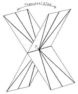
Figure 2: The type I and II solutions for $N=12$ form two sheets related by transposition. The sheets intersect in an affine family, and each sheet contains three additional affine families all passing through the Fourier matrix, where the linear span of the tangent vectors of the two sheets has a dimension equal to its linear defect.

Now we have computed the linear defect $d_{1}$ for a few randomly chosen members of each affine family. For the self-cognate family we find $d_{1}=17$. We observe that $13+13-9=17$, which means that the dimension of the linear span of the tangent vectors of the intersecting solutions of type I and II is equal to the linear defect $d_{1}=17$ of the self-cognate family in which they intersect. For the remaining affine families we find by sampling a large number of members that $d_{1}=13$ (except at the Fourier matrix itself), which is consistent with the fact that these families sit within a 13-dimensional family. It also provides some evidence that the solutions of types I and II exist also far away from the Fourier matrix.

9. $N=p_{1}p_{2}^{2}$, and other choices of $N$

Let us assume that $N=p_{1}p_{2}^{2}$, where $p_{1}$ and $p_{2}$ are prime numbers. We are then able to formulate a precise conjecture concerning how the type I and II solutions found for $N=12$ generalise. Thus we suggest that when $N=p_{1}p_{2}^{2}$ there are always two types of solutions, giving rise to families of Hadamard matrices related to each other by transposition. The conjectured solutions are given by

$$\mbox{Type I :}\hskip 25.60747ptx_{i,j}=x_{i+p_{2},j}\hskip 14.22636pt\mbox{if}\hskip 14.22636pt\mbox{gcd}(j,N)=p_{2}^{2}\$$ (103)

$$\mbox{Type II :}\hskip 22.76219ptx_{i,j}=x_{i+1,j}\hskip 14.22636pt\mbox{if}\hskip 14.22636pt\mbox{gcd}(j,N)=p_{1}\ .$$ (104)

The evidence for this conjecture is primarily that these conditions solve all consistency conditions up to fourth order not only for $N=12$—where they are equivalent to eqs. (90) and (92), respectively—but for all such $N\leq 50$ (namely for $N=3\cdot 2^{2},5\cdot 2^{2},7\cdot 2^{2},11\cdot 2^{2},2\cdot 3^{2},5\cdot 3^{2}$, and $2\cdot 5^{2}$). But we can add some additional evidence.

First of all, although we have continued the calculation to higher orders only for the case $N=12$, we note that the existence of a four parameter family for $N=6$ implies the existence of 22-dimensional family for $N=18$, via the Diţă construction. Compare eq. (101). This is precisely the dimension implied by our conjecture in this case.

Moreover the overall picture gained in the $N=12$ case seems to repeat itself. In general, eqs. (103) or (104) impose $(p_{1}-1)p_{2}(p_{2}-1)$ conditions on the first order solution. If the conjecture is true it implies that the type I and II solutions have dimension

$$d=d_{1}-N\left(1-\frac{1}{p_{1}}\right)\left(1-\frac{1}{p_{2}}\right)\ ,$$ (105)

where $d_{1}$ is the linear defect of the Fourier matrix. Using the expression for $d_{1}$ that we quote in eq. (111), the dimension $d$ can alternatively be expressed as

$$d=d_{A}+N\left(1-\frac{1}{p_{1}}\right)\left(1-\frac{1}{p_{2}}\right)\ ,$$ (106)

where $d_{A}$ is the dimension of the largest affine family obtainable from the Diţă construction in these dimensions. See eq. (115) in Appendix A for this. It follows that

$$d=\frac{d_{1}+d_{A}}{2}\hskip 14.22636pt\Leftrightarrow\hskip 14.22636ptd_{1}=2d-d_{A}\ .$$ (107)

What this equation says is that the conjectured dimension $d$ is just right for the two solutions to intersect in a self-cognate affine family of dimension $d_{A}$, in such a way that the linear span of their tangent vectors equals the linear defect at their intersection.

Using the Diţă construction we obtained one self-cognate family and three pairs of affine families related by transposition, all of dimension $d_{A}$, for all $N=p_{1}p_{2}^{2}$. The details are in Appendix A. For $N=12$ it is known that these are all affine families of maximal dimension stemming from the Fourier matrix [3]. For our seven examples with $N=p_{1}p_{2}^{2}\leq 50$ we checked that the self-cognate family sits in the intersection of the two solutions of type I and II, while the other affine families are contained in a single such solution. We also computed the defect along all these affine families for some randomly chosen matrices, and found that their linear defect equals $2d-d_{A}$ for the self-cognate family, and it equals $d$ for the other families (except at the Fourier matrix itself). This clearly supports the conjecture that the solutions of type I and II survive to higher orders.

Finally, a word about the equations that we actually encounter. As in the case of $N=12$ we know that the fourth order consistency conditions admit other solutions besides the ones that we denote types I and II. For $N=20$ we found the general solution at fourth order. In this case the equations depend on the variables only through combinations similar to those given in eqs. (76), on

$$x_{0,5}-x_{1,5}-x_{3,5}+x_{4,5}\ ,\hskip 17.07164pt4x_{0,5}-x_{1,5}-x_{2,5}-x_{3,5}-x_{4,5}\ ,$$ (108)

and on cyclic permutations of these. Besides the two 25 dimensional solutions of types I and II there exists a 29-dimensional solution which is self-cognate (as an algebraic variety). However, it may well be that such additional solutions are subject to further restrictions at higher orders, as is indeed the case for $N=12$. They may be entirely spurious.

About dimensions $N$ not of the form $p_{1}p_{2}^{2}$ (or $p^{k}$) we have little to say. We have found some hints that eq. (106) may give the dimension of a family of Hadamard matrices in somewhat greater generality, notably if $N=p_{1}p_{2}^{k}$ and $k>1$. The case $N=p_{1}p_{2}$ works in a different way however.

10. Conclusions and speculations

We have investigated the dimension of any smooth set of $N\times N$ complex Hadamard matrices including the Fourier matrix. Our method uses a perturbative expansion in which a linear system is solved at each order. At each order a set of non-linear consistency conditions on the lower order solution must be satisfied. An interesting feature is that we first solve the complexified equations, and then impose unitarity order by order on the solution.

We state our results for the set of dephased Hadamard matrices. If $N$ is a prime number this set consists of a single matrix, namely the Fourier matrix itself. If $N$ is a power of a prime number the dimension of the set is known from previous work, because there are explicit constructions of affine families that saturate the bound given by the first order calculation [18]; see Appendix B for an explicit construction. For $N=6$ our calculations support, to 100th order in perturbation theory, the conjecture that the dimension equals 4. If this is so, it follows that the dimension for $N=12$ is at least 13. Our calculations—carried to 11th order in perturbation theory—support this number, and indeed they prove that the dimension cannot exceed 13 due to consistency conditions that appear at order 4. Moreover an appealing structure emerged, in which the known affine families find a natural place. First order calculations along these families provide evidence that the 13-dimensional families remain 13-dimensional also far away from the Fourier matrix.

For all non-prime power values of $N$ with the single exception of $N=6$, we found that non-trivial consistency conditions arise in the calculation. Our conclusion is that the consistency conditions on the first order solution are identically satisfied if $N=6$ or if $N$ is a prime power, that non-trivial consistency conditions appear at order 11 if $N=10$, at order 7 if $N$ is twice an odd prime with $N>10$, at order 5 if $N$ is a product of two odd primes, at order 4 if $N$ is a product of two primes with at least one prime factor repeated, and at order 3 if $N$ contains three different prime factors. Our evidence for this statement was described in section 7. Based on it we confidently suggest that a systematic understanding of these calculations is possible for arbitrary $N$, even though this is out of our reach at the moment.

It is interesting to observe that 6, and to some extent 10, dimensions stand out as being very special. The conjecture that complete sets of Mutually Unbiased Bases do not exist in any non-prime power dimension rests on numerical searches for $N=6$; see ref. [19] and references therein.

When the consistency conditions break down we know that the dimension of the solution space is less than that suggested by the linear defect. However, in order to see by how much the dimension drops it is necessary to solve these conditions—which are multivariate polynomial equations. We were able to deal with this problem for altogether seven examples where $N$ is of the form $p_{1}p_{2}^{2}$. Based on the results described in sections 8 and 9 we were then able to conjecture the form of a solution for all $N=p_{1}p_{2}^{2}$. The conjectured solution consists of two families of dimension

$$d=\frac{d_{1}+d_{A}}{2}=3N-3p_{1}p_{2}-2p_{2}^{2}+p_{2}+1\ ,$$ (109)

where $d_{1}$ is the linear defect and $d_{A}$ the maximal dimension of known affine families. These two families are related by transposition and intersect in a self-cognate affine family of dimension $d_{A}$, as illustrated in Fig. 2. There are other affine families contained within a single branch of the solution.

We are not sure whether other solutions exist, or not. Indeed this is as far as we have been able to go. We have no hints for what a completely general formula for the dimension of the set of Hadamard matrices containing the Fourier matrix will look like. Nevertheless the evidence strongly suggests that one can be found. We find it intriguing that our results depend on the number theoretical properties of the dimension in such an intricate way.

Acknowledgements: We thank Markus Grassl, Bengt Karlsson, Łukasz Skow- ronek, Feri Szöllősi, Wojtek Tadej, and Karol Życzkowski for sharing their knowledge, and a not so anonymous referee for exceptionally detailed criticism. IB is supported by the Swedish Research Council under contract VR 621-2010-4060.

Appendix A: Background information

Equivalences: In the classification of complex Hadamard matrices two matrices $H_{1},H_{2}$ are regarded as equivalent, written $H_{1}\approx H_{2}$, if there exist diagonal matrices $D_{L},D_{R}$ and permutation matrices $P_{L},P_{R}$ such that

$$H_{2}=D_{L}P_{L}H_{1}P_{R}D_{R}\ .$$ (110)

This is a natural equivalence relation in many applications [2]. If the Hadamard matrices are given in dephased form only discrete equivalences remain. In practice it is hard to take all of them into account.

For composite $N=N_{1}N_{2}$ one finds that the Fourier matrix $F_{N}\approx F_{N_{1}}\otimes F_{N_{2}}$ if and only if $N_{1}$ and $N_{2}$ are relatively prime. Since $F_{N}$ is the character table of the cyclic group $Z_{N}$ this follows from a well known fact about cyclic groups.

The linear defect: Here we just want to mention that the formula for the linear defect, eq. (5), can be rewritten in the form

$$d_{1}=\left(1+k_{1}-\frac{k_{1}}{p_{1}}\right)\left(1+k_{2}-\frac{k_{2}}{p_{2}}\right)\cdot\dots\cdot\left(1+k_{n}-\frac{k_{n}}{p_{n}}\right)N-2N+1\ ,$$ (111)

where it was assumed that the prime number decomposition of $N$ is $N=p_{1}^{k_{1}}\cdot p_{2}^{k_{2}}\cdot\dots\cdot p_{n}^{k_{n}}$ [12].

Affine families: A family of Hadamard matrices stemming from a Hadamard matrix $H$ is said to be affine [3] if it can be written in the form

$$H(a,b,\dots)=H\circ\mbox{EXP}(iR)\ ,$$ (112)

where the product is the entrywise Hadamard product, the exponentiation is entrywise too, and $R$ belongs to a subspace of the set of all real $N\times N$ matrices. The parameters $a,b,\dots$ parametrise that linear subspace. The family is given in dephased form if $H$ is dephased and $R$ has only zeroes in the first row and column. The affine family itself has the topology of a multi-dimensional real torus.

An example for $N=6$ is [2]

$$F(a,b)=\frac{1}{\sqrt{6}}\left(\begin{array}[]{cccccc}1&1&1&1&1&1\\ 1&\omega e^{ia}&\omega^{2}e^{ib}&\omega^{3}&\omega^{4}e^{ia}&\omega^{5}e^{ib}\\ 1&\omega^{2}&\omega^{4}&1&\omega^{2}&\omega^{4}\\ 1&\omega^{3}e^{ia}&e^{ib}&\omega^{3}&e^{ia}&\omega^{3}e^{ib}\\ 1&\omega^{4}&\omega^{2}&1&\omega^{4}&\omega^{2}\\ 1&\omega^{5}e^{ia}&\omega^{4}e^{ib}&\omega^{3}&\omega^{2}e^{ia}&\omega e^{ib}\end{array}\right)\ ,\hskip 22.76219pt\omega=e^{\frac{2\pi i}{6}}\ .$$ (113)

Here $a$ and $b$ are phases that can be chosen freely. The corresponding matrix $X$ is given to first order in eq. (52). Taking the transpose of the matrices in $F(a,b)$ yields another affine family intersecting the first in the Fourier matrix.

The Diţă construction: There exists a construction due to Diţă [18] allowing us to construct an affine family in dimension $N=N_{1}N_{2}$ starting from one Hadamard matrix $H^{(0)}$ in dimension $N_{1}$ and $N_{1}$ possibly different Hadamard matrices $H^{(1)},\dots,H^{(N_{1})}$ in dimension $N_{2}$. In dephased form

$$H=\left(\begin{array}[]{cccc}H^{(0)}_{0,0}H^{(1)}&H^{(0)}_{0,1}D^{(1)}H^{(2)}&\dots&H^{(0)}_{0,N_{1}-1}D^{(N_{1}-1)}H^{(N_{1})}\\ \vdots&\vdots&&\vdots\\ H^{(0)}_{N_{1}-1,0}H^{(1)}&H^{(0)}_{N_{1}-1,1}D^{(1)}H^{(2)}&\dots&H^{(0)}_{N_{1}-1,N_{1}-1}D^{(N_{1}-1)}H^{(N_{1})}\end{array}\right)$$ (114)

where $D^{(1)},\dots,D^{(N_{1}-1)}$ are diagonal unitary matrices (with their first entries equal to one in order to obtain $H$ in dephased form).

Now let $N=p_{1}^{k_{1}}\cdot p_{2}^{k_{2}}\cdot\dots\cdot p_{n}^{k_{n}}$ be the prime number decomposition of $N$. Using the Fourier matrices $F_{p_{1}},\dots,F_{p_{n}}$ as seeds in the Diţă construction it is easy to show that we obtain an affine family of dimension

$$d_{A}=(k_{1}+\dots+k_{n}-1)N-k_{1}\frac{N}{p_{1}}-\dots-k_{n}\frac{N}{p_{n}}+1\ .$$ (115)

This is the dimension of the largest affine family obtainable in this way. But does it contain the Fourier matrix $F_{N}$?

Consider an affine family in dimension $N=N_{1}N_{2}$ obtained from the Diţă construction by setting $H^{(0)}=F_{N_{1}}$, $H^{(1)}=...=H^{(N_{1})}=F_{N_{2}}$ in eq. (114). If the parameters in the diagonal matrices $D^{(k)}$ are chosen so that they become identity matrices we obtain the matrix $F_{N_{1}}\otimes F_{N_{2}}$. But this family also contains a matrix equivalent to $F_{N}$. To see this, let

$$0\leq r,s<N_{1}\ ,\hskip 28.45274pt0\leq m,n<N_{2}\ ,$$ (116)

$$\omega=e^{\frac{2\pi i}{N}}\ ,\hskip 14.22636ptq_{1}=\omega^{N_{2}}\ ,\hskip 14.22636ptq_{2}=\omega^{N_{1}}\ ,$$ (117)

and introduce $N_{1}-1$ diagonal unitaries

$$D^{(r)}=\mbox{diag}(1,x_{1}^{(r)},\dots,x_{N_{2}-1}^{(r)})\ .$$ (118)

The Diţă construction gives rise to a Hadamard matrix $H$ with matrix elements

$$H_{rN_{2}+m,sN_{2}+n}=\frac{1}{\sqrt{N}}x_{m}^{(s)}q_{1}^{rs}q_{2}^{mn}\ .$$ (119)

We now perform a column permutation and obtain an equivalent Hadamard matrix $H^{\prime}$ with matrix elements

$$H^{\prime}_{rN_{2}+m,nN_{1}+s}=\frac{1}{\sqrt{N}}x_{m}^{(s)}q_{1}^{rs}q_{2}^{mn}\ .$$ (120)

The Fourier matrix has the elements

$$\frac{1}{\sqrt{N}}\omega^{ij}=\frac{1}{\sqrt{N}}\omega^{(rN_{2}+m)(nN_{1}+s)}=\frac{1}{\sqrt{N}}\omega^{ms}q_{1}^{rs}q_{2}^{mn}\ ,$$ (121)

and is obtained from $H^{\prime}$ by setting

$$x_{m}^{(s)}=\omega^{ms}\ .$$ (122)

In prime power dimensions the affine family interpolates between the non-equivalent matrices $F_{N}$ and $F_{p}\otimes\dots\otimes F_{p}$.

For $N=p^{k}$ the dimension $d_{A}$ equals the linear defect $d_{1}$ of the Fourier matrix, so affine families of larger dimensions cannot contain it. We believe that this is so for all $N$; it is known to be so for $N\leq 18$ [3, 20]. Affine families not including the Fourier matrix, and not obtainable from the Diţă construction, are known [21].

Self-cognate affine families: By definition [3] a self-cognate family of Hadamard matrices goes into itself under transposition. In section 9 we use the fact that self-cognate affine families of dimension $d_{A}$ exist whenever $N=p_{1}p_{2}^{2}$. To prove this let

$$0\leq r,s<p_{1}\ ,\hskip 28.45274pt0\leq m,n,u,v<p_{2}\ .$$ (123)

We assume that the Diţă construction has already been applied to construct a $p_{1}p_{2}\times p_{1}p_{2}$ Hadamard matrix, as in eq. (120). In the next step we use $p_{2}$ matrices of this type, and moreover the diagonal unitaries used in the first step are allowed to differ from each other. Thus there are $(p_{1}-1)p_{2}$ diagonal unitaries $D^{(s,v)}$ from the first step, and an additional $p_{2}-1$ diagonal unitaries

$$d^{(v)}=\mbox{diag}(1,y_{1}^{(v)},\dots,y_{p_{1}p_{2}-1}^{(v)})\ .$$ (124)

Using $H^{(0)}=F_{p_{2}}$, with matrix elements $q_{2}^{uv}/\sqrt{p_{2}}$, the Diţă construction now gives a Hadamard matrix with matrix elements

$$H_{p_{1}p_{2}u+rp_{2}+m,p_{1}p_{2}v+np_{1}+s}=\frac{1}{\sqrt{N}}q_{1}^{rs}q_{2}^{mn+uv}x_{m}^{(s,v)}y_{rp_{2}+m}^{(v)}\ .$$ (125)

We next perform a column permutation according to

$$H^{\prime}_{p_{1}p_{2}u+rp_{2}+m,p_{1}p_{2}n+sp_{2}+v}=\frac{1}{\sqrt{N}}q_{1}^{rs}q_{2}^{mn+uv}x_{m}^{(s,v)}y_{rp_{2}+m}^{(v)}$$ (126)

These are the matrix elements of the matrix $H^{\prime}(x,y)$. We want to prove that for all choices of the parameters $x,y$ we can find some parameters $\tilde{x},\tilde{y}$ such that $H^{\prime}(x,y)^{\rm T}=H^{\prime}(\tilde{x},\tilde{y})$. Transposition of $H^{\prime}$ is given by

$$u\leftrightarrow n\ ,\hskip 14.22636ptr\leftrightarrow s\ ,\hskip 14.22636ptm\leftrightarrow v\ ,$$ (127)

and by

$$x_{m}^{(s,v)}\rightarrow x_{v}^{(r,m)}\ ,\hskip 28.45274pty_{rp_{2}+m}^{(v)}\rightarrow y_{sp_{2}+v}^{(m)}\ .$$ (128)

So we set

$$\tilde{x}^{(s,v)}_{m}=y_{sp_{2}+v}^{(m)}\ ,\hskip 22.76219pt\tilde{y}_{rp_{2}+m}^{(v)}=x_{v}^{(r,m)}\ ,$$ (129)

which is always possible. This proves that the family is self-cognate.

Other affine families: One obtains affine families that do not go into themselves under transposition if one performs the Diţă construction in a different order. The self-cognate family was obtained by starting with a matrix of size $p_{2}$, enlarging it to size $p_{1}p_{2}$, and finally to size $p_{2}p_{1}p_{2}$. Other examples referred to in section 9 are obtained from the sequences $p_{2}\rightarrow p_{2}^{2}\rightarrow p_{1}p_{2}^{2}$ and $p_{1}\rightarrow p_{2}p_{1}\rightarrow p_{2}^{2}p_{1}$, and they lead to affine families of the same dimension. In the special case of $N=12$ all affine families of maximal dimension are known [3], and we have proved that all of them can be obtained from some variant of the Diţă construction.

The case $N=6$: A number of non-affine families of $6\times 6$ Hadamard matrices have been found [22, 23, 24, 17], and all analytically known families are included as subfamilies of the 3-dimensional non-affine family found by Karlsson [13]. As mentioned in the introduction it is known that a 4-dimensional family exists [5], but a proof that this family includes the Fourier matrix is missing. It is also known that at least one isolated Hadamard matrix, not belonging to this family, exists [25, 26].

Families not including $F_{N}$: Finally, to avoid any misunderstanding, we observe that although the defect vanishes for $N=7$ (say), this does not mean that the Fourier matrix is the only known Hadamard matrix in this case. Indeed a one-dimensional affine family not including the Fourier matrix is known for $N=7$, and for some other cases where $N$ is a prime equal to 1 modulo 6 [27]. We have nothing to say about such families.

Appendix B: The prime power case

When $N=p^{k}$ is a power of a prime $p$ the Diţă construction allows us to construct an affine family of maximal dimension equal to the linear defect $d_{1}$. A more direct construction is the following. The matrix elements of $R$, in eq. (112), are given in terms of independent parameters $\phi_{n,i,j}$ as

$$R_{ij}=\sum_{n=0}^{k}\phi_{n,i\ {\rm mod}\ p^{n},j\ {\rm mod}\ p^{k-n}}\ ,\hskip 28.45274pt\phi_{n,i,j}=0\ \ \mbox{if}\ \ i<p^{n-1}\ .$$ (130)

Dephased matrices are obtained by excluding $n=0$ and $n=k$ from the sum, and setting $\phi_{n,i,0}=0$, that is

$$R_{ij}=\sum_{n=1}^{k-1}\phi_{n,i\ {\rm mod}\ p^{n},j\ {\rm mod}\ p^{k-n}}\ ,\hskip 17.07164pt\phi_{n,i,j}=0\ \ \mbox{if}\ \ i<p^{n-1}\ \mbox{or}\ j=0\ .$$ (131)

The modular arithmetic means that $R$ splits into $p\times p$ equal blocks of size $p^{k-1}$. It is obtained by adding the matrices $\phi_{n}$ together, and the number of entries in these matrices taken together is

$$\sum_{n=1}^{k-1}(p^{n}-p^{n-1})(p^{k-n}-1)=(k-1)p^{k}-kp^{k-1}+1=d_{1}\ .$$ (132)

Since $\phi_{n,i,j}$ repeats for $i\geq p^{n}$ while $\phi_{n+1,i,j}=0$ for $i<p^{n}$, these entries are indeed the independent parameters on which the matrix $R$ depends. The proof that the resulting matrices are unitary Hadamard matrices is not entirely straightforward, but we omit it here.

The connection to the parametrisation we use in the main body of the paper is easily found for the special case $N=p^{2}$. We simply compute $X={\bf 1}-HF^{\dagger}$, and find for its matrix elements that

$$X_{i\ {\rm mod}\ p,rp\ {\rm mod}\ N}=-\frac{1}{p}\sum_{k=0}^{p-1}\omega^{-pkr}e^{i\phi_{1,i\ {\rm mod}\ p,k\ {\rm mod}\ p}}\ .$$ (133)

From this we learn that the choice of free parameters that we make in the perturbative construction may not be the optimal one for a closed form expression.

Appendix C: The consistency conditions hold to second order

We mention in the text that the consistency conditions (54) always hold to second order. We give the key steps in the proof here since they serve to illustrate the complexities involved in making a calculation valid for all $N$. In particular we need to make a liberal use of linear congruence relations.

Setting $s=2$ in eq. (39) and replacing $X^{(1)}$ by its solution (50) we obtain

$$B_{i,i}^{(2,n)}=\hskip 199.16928pt$$

(134)

$$=\sum_{k=0}^{N-1}\left[x^{(1)}_{(i+n)\ {\rm mod}\ {\rm gcd}(k-n,N),k-n}-x^{(1)}_{i\ {\rm mod}\ {\rm gcd}(k-n,N),k-n}\right]x^{(1)}_{i\ {\rm mod}\ {\rm gcd}(k,N),-k}\ .$$

At second order therefore the consistency conditions (54) are

$$0=\sum_{q=0}^{\frac{N}{{\rm gcd}(n,N)}-1}\sum_{k=0}^{N-1}x^{(1)}_{(i+q\ {\rm gcd}(n,N))\ {\rm mod\ gcd}(k,N),-k}\times\hskip 71.13188pt$$

(135)

$$\times\left[x^{(1)}_{(i+q\ {\rm gcd}(n,N)+n)\ {\rm mod}\ {\rm gcd}(k-n,N),k-n}-x^{(1)}_{(i+q\ {\rm gcd}(n,N))\ {\rm mod}\ {\rm gcd}(k-n,N),k-n}\right]\ .$$

The crucial step is to realise that the first factor is the same for two values of $q$ whenever their difference $\Delta q$ obeys

$$\Delta q\ \mbox{gcd}(n,N)=0\ \ \mbox{mod gcd}(k,N)\ .$$ (136)

This will permit us to break the sum over $q$ into two, one of which involves only the second factor.

The smallest solution for $\Delta q$ is

$$\Delta q=\frac{\mbox{lcm}\left(\mbox{gcd}(n,N),\mbox{gcd}(k,N)\right)}{\mbox{gcd}(n,N)}=\frac{\mbox{gcd}\left(\mbox{lcm}(n,k),N\right)}{\mbox{gcd}(n,N)}\ ,$$ (137)

where lcm denotes the least common multiple. Write $q=q_{1}+\Delta q\ q_{2}$. The consistency condition then takes the form

$$0=\sum_{k=0}^{N-1}\sum_{q_{1}=0}^{\frac{{\rm gcd}({\rm lcm}(n,k),N))}{{\rm gcd}(n,N)}-1}x^{(1)}_{(i+q_{1}\ {\rm gcd}(n,N))\ {\rm mod\ gcd}(k,N),-k}\times\hskip 42.67912pt$$

(138)

$$\times\sum_{q_{2}=0}^{\frac{N}{{\rm gcd}({\rm lcm}(n,k),N)}-1}\Large[x^{(1)}_{(i+q_{1}\ {\rm gcd}(n,N)+q_{2}\ {\rm gcd}({\rm lcm}(n,k),N)+n)\ {\rm mod}\ {\rm gcd}(k-n,N),k-n}-$$

$$-x^{(1)}_{(i+q_{1}\ {\rm gcd}(n,N)+q_{2}\ {\rm gcd}({\rm lcm}(n,k),N))\ {\rm mod}\ {\rm gcd}(k-n,N),k-n}\Large]\ .$$

The dependence on $q_{2}$ is now isolated to the sum that constitutes the second factor, and it is enough to show that this sum vanishes. Indeed the terms will cancel in pairs if for each $q_{2}$ we can find a $q_{2}+\Delta q_{2}$ such that

$$\left\{\Delta q_{2}\ \mbox{gcd}({\rm lcm}(n,k),N)=n\right\}\ \ \mbox{mod gcd}(k-n,N)\ .$$ (139)

This is what we need, because although $q_{2}$ and $\Delta q_{2}$ are defined modulo $N/{\rm gcd}({\rm lcm}(n,k),N)$ they appear multiplied by ${\rm gcd}({\rm lcm}(n,k),N)$ in eq. (138). We know that the equation $xa=y$ taken modulo $b$ has a solution if and only if gcd$(a,b)$ divides $y$. So we must show that $n$ is divisible by

$$\mbox{gcd}\left(\mbox{gcd}(\mbox{lcm}(n,k),N),\mbox{gcd}(k-n,N)\right)=\mbox{gcd}\left(\mbox{lcm}(n,k),k-n,N)\right)\ .$$ (140)

It is enough to show that $n$ is divisible by $\mbox{gcd}\left(\mbox{lcm}(n,k),k-n\right)$. But this is so because

$$\mbox{gcd}\left(\mbox{lcm}(n,k),k-n\right)=\mbox{lcm}\left(\mbox{gcd}(n,k-n),\mbox{gcd}(k,k-n)\right)=\mbox{gcd}(n,k)\$$ (141)

which certainly divides $n$. This ends the proof.

Appendix D: A toy model

The description of our method in section 2 may appear forbidding, so in this Appendix we apply it to the simple example

$$f(X,Y)=X\left(X-1\right)^{2}-\left({\rm e}^{Y}-1\right)^{2}=0\ .$$ (142)

Since there are only two variables we streamline the notation a little. The two solutions $\left(X,Y\right)=\left(0,0\right)$ and $\left(X,Y\right)=\left(1,0\right)$ are obvious by inspection. We shall work up to order $4$.

For the first solution we expand eq. (142) around the origin:

$$f(X,Y)=X-2X^{2}+X^{3}-Y^{2}-Y^{3}-7Y^{4}/12+\dots\ .$$ (143)

We next collect $X$ and $Y$ into a vector and expand it as in eq. (7),

$$\left[\begin{array}[]{c}X\\ Y\end{array}\right]=\left[\begin{array}[]{c}X_{\left(1\right)}\\ Y_{\left(1\right)}\end{array}\right]+\left[\begin{array}[]{c}X_{\left(2\right)}\\ Y_{\left(2\right)}\end{array}\right]+\left[\begin{array}[]{c}X_{\left(3\right)}\\ Y_{\left(3\right)}\end{array}\right]+\left[\begin{array}[]{c}X_{\left(4\right)}\\ X_{\left(4\right)}\end{array}\right]+\dots\ .$$ (144)

We then obtain eqs. (9-12) in the form

$$X_{\left(1\right)} = 0\hskip 193.47873pt\equiv B_{(1)}$$ (145)

$$X_{\left(2\right)} = 2X_{\left(1\right)}^{2}+Y_{\left(1\right)}^{2}\hskip 139.4185pt\equiv B_{\left(2\right)}$$ (146)

$$X_{\left(3\right)} = -X_{\left(1\right)}^{3}+4X_{\left(1\right)}X_{\left(2\right)}+Y_{\left(1\right)}^{3}+2Y_{\left(1\right)}Y_{\left(2\right)}\hskip 17.07164pt\equiv B_{\left(3\right)}$$ (147)

$$X_{\left(4\right)} = 2X_{\left(2\right)}^{2}+4X_{\left(1\right)}X_{\left(3\right)}-3X_{\left(1\right)}^{2}X_{\left(2\right)}+Y_{\left(2\right)}^{2}+$$ (148)

$$+2Y_{\left(1\right)}Y_{\left(3\right)}+3Y_{\left(1\right)}^{2}Y_{\left(2\right)}+7Y_{\left(1\right)}^{4}/12\hskip 34.1433pt\equiv B_{\left(4\right)}\ .$$

At each order this is the linear system $AX_{(n)}=B_{(n)}$, where $A=\left[\begin{array}[]{cc}1&0\end{array}\right]$. The linear defect is the number of variables minus the rank of $A$, and equals $1$.

We choose the Moore-Penrose pseudo-inverse

$$\hat{A}=\left[\begin{array}[]{c}1\\ 0\end{array}\right]\quad,\quad 1-\hat{A}A=\left[\begin{array}[]{cc}0&0\\ 0&1\end{array}\right]\quad,\quad 1-A\hat{A}=0\ .$$ (149)

In our solution (15) we denote the components of the arbitrary vector $Z$ by $x_{(n)}$ and $y_{(n)}$, and obtain at each order

$$\left[\begin{array}[]{c}X_{\left(n\right)}\\ Y_{\left(n\right)}\end{array}\right]=\left[\begin{array}[]{c}1\\ 0\end{array}\right]\left[B_{\left(n\right)}\right]+\left[\begin{array}[]{cc}0&0\\ 0&1\end{array}\right]\left[\begin{array}[]{c}x_{\left(n\right)}\\ y_{\left(n\right)}\end{array}\right]=\left[\begin{array}[]{c}B_{\left(n\right)}\\ y_{\left(n\right)}\end{array}\right]\ .$$ (150)

There are no consistency conditions, which means that the defect remains $1$ to all orders. Hence the solution is one-dimensional and unique around this point.

We have $B_{(1)}=0$, and the remaining $B_{(n)}$ are computed recursively. To order 4 we obtain

$$\left[\begin{array}[]{c}X\\ Y\end{array}\right] = \left[\begin{array}[]{c}\left\{\begin{array}[]{c}y_{\left(1\right)}^{2}+y_{\left(1\right)}^{3}+2y_{\left(1\right)}y_{\left(2\right)}+y_{\left(2\right)}^{2}+\\ +2y_{\left(1\right)}y_{\left(3\right)}+3y_{\left(1\right)}^{2}y_{\left(2\right)}+31y_{\left(1\right)}^{4}/12\end{array}\right\}\\ y_{\left(1\right)}+y_{\left(2\right)}+y_{\left(3\right)}+y_{\left(4\right)}\end{array}\right]\ .$$ (157)

Setting $t=y_{\left(1\right)}+y_{\left(2\right)}+y_{\left(3\right)}+y_{\left(4\right)}$ our first solution is, to order 4,

$$\left[\begin{array}[]{c}X\\ Y\end{array}\right] \approx \left[\begin{array}[]{c}t^{2}+t^{3}+31t^{4}/12\\ t\end{array}\right]\ .$$ (162)

Next we expand around the solution $(X,Y)=(1,0)$. After shifting the variable $X$, and expanding around the new origin, we get

$$f(X,Y)=X^{2}+X^{3}-Y^{2}-Y^{3}-7Y^{4}/12+\dots=0\ .$$ (163)

Again we expand $X$ and $Y$ as in eq. (7) and obtain eqs. (9-12) in the form

$$0 = 0\hskip 199.16928pt\equiv B_{(1)}$$ (164)

$$0 = -X_{\left(1\right)}^{2}+Y_{\left(1\right)}^{2}\hskip 142.26378pt\equiv B_{(2)}$$ (165)

$$0 = -X_{\left(1\right)}^{3}-2X_{\left(1\right)}X_{\left(2\right)}+Y_{\left(1\right)}^{3}+2Y_{\left(1\right)}Y_{\left(2\right)}\hskip 22.76219pt\equiv B_{(3)}$$ (166)

$$0 = -X_{\left(2\right)}^{2}-2X_{\left(1\right)}X_{\left(3\right)}-3X_{\left(1\right)}^{2}X_{\left(2\right)}+Y_{\left(2\right)}^{2}+$$ (167)

$$+2Y_{\left(1\right)}Y_{\left(3\right)}+3Y_{\left(1\right)}^{2}Y_{\left(2\right)}+7Y_{\left(1\right)}^{4}/12\hskip 39.83385pt\equiv B_{(4)}\ .$$

We have obtained the linear systems $AX_{(n)}=B_{(n)}$, where $A=\left[\begin{array}[]{cc}0&0\end{array}\right]$. Again we use the Moore-Penrose inverse

$$\hat{A}=\left[\begin{array}[]{c}0\\ 0\end{array}\right]\quad,\quad 1-\hat{A}A=\left[\begin{array}[]{cc}1&0\\ 0&1\end{array}\right]\quad,\quad 1-A\hat{A}=1\ .$$ (168)

Our solution (15) becomes

$$\left[\begin{array}[]{c}X_{\left(n\right)}\\ Y_{\left(n\right)}\end{array}\right]=\left[\begin{array}[]{c}0\\ 0\end{array}\right]\left[B_{\left(n\right)}\right]+\left[\begin{array}[]{cc}1&0\\ 0&1\end{array}\right]\left[\begin{array}[]{c}x_{\left(n\right)}\\ y_{\left(n\right)}\end{array}\right]=\left[\begin{array}[]{c}x_{\left(n\right)}\\ y_{\left(n\right)}\end{array}\right]\ ,$$ (169)

subject to the consistency condition (14), which takes the form

$$B_{\left(n\right)}=0$$ (170)

The linear defect is $2$. Since the solutions (169) have no heterogeneous component, all we have to do is to study the consistency conditions. To second order this is

$$B_{\left(2\right)}=-X_{\left(1\right)}^{2}+Y_{\left(1\right)}^{2}=-x_{\left(1\right)}^{2}+y_{\left(1\right)}^{2}=0\ ,$$ (171)

with two solutions

$$\mathrm{I.}\quad y_{\left(1\right)} = x_{\left(1\right)}$$ (172)

$$\mathrm{II.}\quad y_{\left(1\right)} = -x_{\left(1\right)}$$ (173)

Therefore the second order defect is $1$.

To third order we have

$$B_{\left(3\right)} = -X_{\left(1\right)}^{3}-2X_{\left(1\right)}X_{\left(2\right)}+Y_{\left(1\right)}^{3}+2Y_{\left(1\right)}Y_{\left(2\right)}=$$ (174)

$$= -x_{\left(1\right)}^{3}-2x_{\left(1\right)}x_{\left(2\right)}+y_{\left(1\right)}^{3}+2y_{\left(1\right)}y_{\left(2\right)}=0\ .$$

For solution I this is

$$B_{\left(3\right)}=\left[\begin{array}[]{cc}-2x_{\left(1\right)}&2x_{\left(1\right)}\end{array}\right]\left[\begin{array}[]{c}x_{\left(2\right)}\\ y_{\left(2\right)}\end{array}\right]=0\quad\Rightarrow\quad y_{\left(2\right)}=x_{\left(2\right)}\ .$$ (175)

This is the unnumbered equation $Uh_{n}^{\left(2\right)}=V$ mentioned at the end of section 2, with $U=\left[\begin{array}[]{cc}-2x_{\left(1\right)}&2x_{\left(1\right)}\end{array}\right]$ and $V=0$. For solution II we get

$$B_{\left(3\right)} = \left[\begin{array}[]{cc}-2x_{\left(1\right)}&-2x_{\left(1\right)}\end{array}\right]\left[\begin{array}[]{c}x_{\left(2\right)}\\ y_{\left(2\right)}\end{array}\right]-2x_{\left(1\right)}^{3}=0$$ (179)

$$\Rightarrow \quad y_{\left(2\right)}=-x_{\left(2\right)}-x_{\left(1\right)}^{2}\ .$$ (180)

Here $U=\left[\begin{array}[]{cc}-2x_{\left(1\right)}&2x_{\left(1\right)}\end{array}\right]$ and $V=2x_{\left(1\right)}^{3}$. At second order we fixed the variable $y_{\left(1\right)}$ and at third order we fixed $y_{(2)}$. No further fixing of first order variables was needed, so the defect remains $1$.

Note that $x_{\left(1\right)}=y_{\left(1\right)}=0$ satisfies both (171) and (174). A further analysis reveals that this leads to special cases of solutions I and II.

To fourth order we have

$$B_{\left(4\right)} = -x_{\left(2\right)}^{2}-2x_{\left(1\right)}x_{\left(3\right)}-3x_{\left(1\right)}^{2}x_{\left(2\right)}+$$ (181)

$$+y_{\left(2\right)}^{2}+2y_{\left(1\right)}y_{\left(3\right)}+3y_{\left(1\right)}^{2}y_{\left(2\right)}+7y_{\left(1\right)}^{4}/12=0$$

For solution I we obtain an equation $Uh_{n}^{\left(3\right)}=V$ of the form

$$B_{\left(4\right)} = \left[\begin{array}[]{cc}-2x_{\left(1\right)}&2x_{\left(1\right)}\end{array}\right]\left[\begin{array}[]{c}x_{\left(3\right)}\\ y_{\left(3\right)}\end{array}\right]+7x_{\left(1\right)}^{4}/12=0$$ (185)

$$\Rightarrow \quad y_{\left(3\right)}=x_{\left(3\right)}-7x_{\left(1\right)}^{3}/24$$ (186)

The same matrix $U=\left[\begin{array}[]{cc}-2x_{\left(1\right)}&2x_{\left(1\right)}\end{array}\right]$ shows up again, while now $V=-7x_{\left(1\right)}^{4}/12$. And for solution II we get

$$B_{\left(4\right)} = \left[\begin{array}[]{cc}-2x_{\left(1\right)}&-2x_{\left(1\right)}\end{array}\right]\left[\begin{array}[]{c}x_{\left(3\right)}\\ y_{\left(3\right)}\end{array}\right]-4x_{\left(1\right)}^{2}x_{\left(2\right)}-17x_{\left(1\right)}^{4}/12=0$$ (190)

$$\Rightarrow \quad y_{\left(3\right)}=-x_{\left(3\right)}-2x_{\left(1\right)}x_{\left(2\right)}-17x_{\left(1\right)}^{3}/24$$ (191)

Again the same matrix $U$ shows up.

And again at this order $y_{\left(3\right)}$ is fixed and no further fixing of first order variables is needed, so the defect remains $1$. Summing up the order-by-order solutions one gets the two solutions

$$\mathrm{I.}\quad\left[\begin{array}[]{c}X\\ Y\end{array}\right]=\left[\begin{array}[]{c}x_{\left(1\right)}+x_{\left(2\right)}+x_{\left(3\right)}+x_{\left(4\right)}\\ x_{\left(1\right)}+x_{\left(2\right)}+x_{\left(3\right)}-7x_{\left(1\right)}^{3}/24+y_{\left(4\right)}\end{array}\right]\approx$$ (196)

$$\approx \left[\begin{array}[]{c}x_{\left(1\right)}+x_{\left(2\right)}+x_{\left(3\right)}\\ \left(x_{\left(1\right)}+x_{\left(2\right)}+x_{\left(3\right)}\right)-7\left(x_{\left(1\right)}+x_{\left(2\right)}+x_{\left(3\right)}\right)^{3}/24\end{array}\right]+\left[\begin{array}[]{c}x_{\left(4\right)}\\ y_{\left(4\right)}\end{array}\right]$$ (208)

$$\mathrm{II.}\quad\left[\begin{array}[]{c}X\\ Y\end{array}\right]=\left[\begin{array}[]{c}x_{\left(1\right)}+x_{\left(2\right)}+x_{\left(3\right)}+x_{\left(4\right)}\\ \left\{\begin{array}[]{c}-x_{\left(1\right)}-x_{\left(2\right)}-x_{\left(1\right)}^{2}-x_{\left(3\right)}-\\ -2x_{\left(1\right)}x_{\left(2\right)}-17x_{\left(1\right)}^{3}/24+y_{\left(4\right)}\end{array}\right\}\end{array}\right]\approx$$

$$\approx \left[\begin{array}[]{c}x_{\left(1\right)}+x_{\left(2\right)}+x_{\left(3\right)}\\ \left\{\begin{array}[]{c}-\left(x_{\left(1\right)}+x_{\left(2\right)}+x_{\left(3\right)}\right)-\left(x_{\left(1\right)}+x_{\left(2\right)}+\right.\\ \left.+x_{\left(3\right)}\right)^{2}-17\left(x_{\left(1\right)}+x_{\left(2\right)}+x_{\left(3\right)}\right)^{3}/24\end{array}\right\}\end{array}\right]+\left[\begin{array}[]{c}x_{\left(4\right)}\\ y_{\left(4\right)}\end{array}\right]$$ (215)

We now compare our results with the known form of the solution, see Fig. 3. Around $\left(X,Y\right)=\left(0,0\right)$ the solution is smooth and unique. We can use the formula for the solution of the cubic and trigonometric identities to write it as

$$X=\frac{4}{3}\sin^{2}\left[\frac{1}{3}\arcsin\left(\frac{3\sqrt{3}}{2}\left(e^{Y}-1\right)\right)\right]\approx Y^{2}+Y^{3}+\frac{31}{12}Y^{4}\ ,$$ (216)

in agreement with eq. (162). At $\left(X,Y\right)=\left(1,0\right)$ there are two intersecting solutions. Around this point it is easy to solve eq. (142) to get

$$\mathrm{I.}\quad Y = \ln\left[1+\left(X-1\right)\sqrt{X}\right]\approx\left(X-1\right)-\frac{7}{24}\left(X-1\right)^{3}$$ (217)

$$\mathrm{II.}\quad Y = \ln\left[1-\left(X-1\right)\sqrt{X}\right]\approx-\left(X-1\right)-\left(X-1\right)^{2}-$$ (218)

$$-\frac{17}{24}\left(X-1\right)^{3}$$

in agreement with eqs. (208) and (215) respectively (if we recall the shift we made in $X$).

Figure 3: Solution to $X\left(X-1\right)^{2}=\left({\rm e}^{Y}-1\right)^{2}$.

One final word about the choice of the homogeneous terms and how it relates to different parametrizations of the solution. By setting all homogeneous terms with $n>1$ to $0$, we are using $Y$ as the free parameter in (162) and $X$ in (208) and (215). But if instead we choose $x_{\left(1\right)}=-t$, $x_{\left(2\right)}=-t^{2}$, $x_{\left(3\right)}=-7t^{3}/24$ in eq. (215) we get

$$\mathrm{II.}\quad\left[\begin{array}[]{c}X\\ Y\end{array}\right]\approx\left[\begin{array}[]{c}-t-t^{2}-7t^{3}/24\\ t\end{array}\right]\ .$$ (219)

This amounts to using $Y$ as the free parameter. In (162) it is clearly impossible to use $X$ as the free parameter (because the curve is tangent to the $Y$ axis here) but one can set $y_{\left(1\right)}=t$, $y_{\left(2\right)}=-t^{2}/2$, $y_{\left(3\right)}=-2t^{3}/3$ and generate the equally valid parametrization

$$\left[\begin{array}[]{c}X\\ Y\end{array}\right]\approx\left[\begin{array}[]{c}t^{2}\\ t-t^{2}/2-2t^{3}/3\end{array}\right]\ .$$ (220)

References

[1] J. J. Sylvester, Thoughts on inverse orthogonal
matrices, simultaneous sign-successions, and tessellated pavements in two
or more colours, with applications to Newton’s rule, ornamental tile-work,
and the theory of numbers, Phil. Mag. 34 (1867) 461.
[2] U. Haagerup, Orthogonal maximal abelian *-subalgebras of the
matrices and cyclic -roots, in Operator Algebras and
Quantum Field Theory, Rome (1996), Internat. Press, Cambridge, MA 1997.
[3] W. Tadej and K. Życzkowski, A concise guide to complex
Hadamard matrices, Open Sys. Inf. Dyn. 13 (2006) 133.
[4] K. J. Horadam: Hadamard Matrices and Their Applications,
Princeton UP, 2007.
[5] F. Szöllősi, Construction, classification
and parametrization of complex Hadamard matrices, Ph D thesis, CEU, Budapest
2011; eprint arXiv:1150.5590.
[6] K. Kraus, Complementary observables and uncertainty
relations, Phys. Rev. D35 (1987) 3070.
[7] T. Durt, B.-G. Englert, I. Bengtsson, and K. Życzkowski,
On Mutually Unbiased Bases, Int. J. Quant. Inf. 8 (2010) 535.
[8] B.-G. Englert, D. Kaszlikowski, L. C. Kwek, and W. H. Chee,
Wave-particle duality in multi-path interferometers: general concepts and
three-path interferometers, Int. J. Quant. Inf. 6 (2008) 129.
[9] R. F. Werner, All teleportation and dense coding schemes,
J. Phys. A34 (2001) 7081.
[10] S. Popa, Orthogonal pairs of subalgebras in finite von
Neumann algebras, J. Operator Theory 9 (1983) 253.
[11] T. Banica and R. Nicoara, Quantum groups and Hadamard
matrices, Panamer. Math. J. 17 (2007) 1.
[12] W. Tadej and K. Życzkowski, The defect of a unitary matrix,
Lin. Alg. Appl. 429 (2008) 447.
[13] B. R. Karlsson, Three-parameter complex Hadamard
matrices of order 6, Lin. Alg. Appl. 434 (2011) 247.
[14] F. Szöllősi, Complex Hadamard matrices of order
6: a four-parameter family, J. London Math. Soc. 85 (2012) 616.
[15] A. J. Skinner, V. A. Newell, and R. Sanchez, Unbiased
bases (Hadamards) for six-level systems: Four ways from Fourier, J. Math. Phys.
50 (2009) 012107.
[16] R. Penrose, A generalized inverse for matrices, Proc.
Camb. Phil. Soc. 51 (1955) 406.
[17] B. R. Karlsson, Two-parameter complex Hadamard
matrices for , J. Math. Phys. 50 (2009) 082104.
[18] P. Diţă, Some results on the parametrization of complex
Hadamard matrices, J. Phys. A37 (2004) 5355.
[19] P. Raynal, X. Lü, and B.-G. Englert, Mutually unbiased
bases in dimension six: The four most distant bases, Phys. Rev. A83
(2011) 062303.
[20] W. Tadej, private communication.
[21] F. Szöllősi, Parametrizing complex Hadamard
matrices, Eur. J. Comb. 29 (2008) 1219.
[22] K. Beauchamp and R. Nicoara, Orthogonal maximal abelian
*-subalgebras of the 6 6 matrices, Lin. Alg. Appl. 428 (2008) 1833.
[23] M. Matolcsi and F. Szöllősi, Towards a
classification of complex Hadamard matrices, Open Sys. Inf.
Dyn. 15 (2008) 93.
[24] F. Szöllősi, A two-parameter family of complex
Hadamard matrices of order 6 induced by hypocycloids, Proc. Amer. Math. Soc.
138 (2010) 921.
[25] A. T. Butson, Generalized Hadamard matrices,
Proc. Am. Math. Soc. 13 (1962) 894.
[26] T. Tao, Fuglede’s conjecture is false in 5 and higher
dimensions, Math. Res. Lett. 11 (2004) 251.
[27] M. Petrescu, Existence of continuous families of
complex Hadamard matrices in certain prime dimensions and related results,
PhD thesis, Univ. of California 1997.