The Strong Decays of Orbitally Excited $B^{*}_{sJ}$ Mesons by Improved Bethe-Salpeter Method

Abstract

We calculate the masses and the strong decays of orbitally excited states $B_{s0}$, $B^{\prime}_{s1}$, $B_{s1}$ and $B_{s2}$ by the improved Bethe-Salpeter method. The predicted masses of $B_{s0}$ and $B^{\prime}_{s1}$ are $M_{B_{s0}}=5.723\pm 0.280~{}{\rm GeV}$, $M_{B^{\prime}_{s1}}=5.774\pm 0.330~{}{\rm GeV}$. We calculate the isospin symmetry violating decay processes $B_{s0}\to B_{s}\pi$ and $B^{\prime}_{s1}\to B_{s}^{*}\pi$ through $\pi^{0}-\eta$ mixing and get small widths. Considering the uncertainties of the masses, for $B_{s0}$ and $B^{\prime}_{s1}$, we also calculate the OZI allowed decay channels: $B_{s0}\to B\bar{K}$ and $B^{\prime}_{s1}\to B^{*}\bar{K}$. For $B_{s1}$ and $B_{s2}$, the OZI allowed decay channels $B_{s1}\to B^{*}\bar{K}$, $B_{s2}\to B\bar{K}$ and $B_{s2}\to B^{*}\bar{K}$ are studied. In all the decay channels, the reduction formula, PCAC relation and low energy theorem are used to estimate the decay widths. We also obtain the strong coupling constants $G_{B_{s0}B_{s}\pi}$, $G_{B_{s0}B\bar{K}}$, $G_{B^{\prime}_{s1}B_{s}^{*}\pi}$, $F_{B^{\prime}_{s1}B_{s}^{*}\pi}$, $G_{B^{\prime}_{s1}B^{*}\bar{K}}$, $F_{B^{\prime}_{s1}B^{*}\bar{K}}$, $G_{B_{s1}B^{*}\bar{K}}$, $F_{B_{s1}B^{*}\bar{K}}$, $G_{B_{s2}B\bar{K}}$ and $G_{B_{s2}B^{*}\bar{K}}$.

Keywords: Strong decay; Orbitally Excited $B^{*}_{sJ}$ Mesons; Improved B-S Method.

I Introduction

The heavy-light mesons play an important role in hadron physics. During the past several years, many heavy-light mesons were observed in experiments. In the Particle Data Group (PDG) table pdg , there are four $P$-wave charm states $D_{0}^{*}(2400)^{0}$, $D_{1}(2420)^{0}$, $D_{1}(2430)^{0}$, $D_{2}^{*}(2460)^{0}$, and two $P$-wave bottom states $B_{1}(5721)^{0}$, $B_{2}^{*}(5747)^{0}$. For the $P$-wave bottom-strange states, $B_{s1}$ and $B_{s2}^{*}$ are observed by the CDF Collaboration in 2008 cdf . Later the D0 Collaboration also reported $B_{s2}^{*}$ d0 . Meanwhile D0 Collaboration indicated that $B_{s1}$ was not observed with the available data set.

In the heavy quark effective theory(HQET) hqet , for the heavy-light meson system, the angular momentum of light quark $j_{l}$ is a good quantum number when the heavy quark have $m_{Q}\to\infty$ limit. They are $j^{P}_{l}={\frac{1}{2}}^{-}$ $H$ doublet ($0^{-},1^{-}$) with orbital angular momentum $L=0$; $j^{P}_{l}={\frac{1}{2}}^{+}$ $S$ doublet ($0^{+},1^{+}$) and $j^{P}_{l}={\frac{3}{2}}^{+}$ $T$ doublet ($1^{+},2^{+}$) with orbital angular momentum $L=1$. The D0 and CDF indicated that $B_{s1}(5830)$ and $B_{s2}^{*}(5840)$ correspond to the states with $J^{P}=1^{+}$ and $J^{P}=2^{+}$ in $T$ doublet cdf ; d0 . While for the $B^{*}_{sJ}$ state with $S$ doublet $J^{P}=(0^{+},1^{+})$ do not have the experimental evidence. For the charm states, $D_{0}^{*}(2400)^{0}$ and , $D_{1}(2430)^{0}$ are the $\frac{1}{2}^{+}$ $S$ doublet ($0^{+},1^{+}$), $D_{1}(2420)^{0}$ and $D_{2}^{*}(2460)^{0}$ belong to $\frac{3}{2}^{+}$ $T$ doublet ($1^{+},2^{+}$). $B_{1}(5721)^{0}$ and $B_{2}^{*}(5747)^{0}$ also belong to $\frac{3}{2}^{+}$ $T$ doublet ($1^{+},2^{+}$).

The observations of these $P$-wave mesons inspire our interest in their nature. There are many theoretical approaches are used to study their properties wangzg ; L4 ; L5 ; qq ; 16 ; liu ; supp ; zhao ; aff ; hill . In this work, we focus on the productions of $P$-wave charm states, bottom states and bottom-strange states in exclusive semileptonic and nonleptonic $B_{c}$ decays.

Since the discovery of $D_{s0}(2317)$ 2317 , the heavy-light orbitally excited states stimulated continued interesting attentions. There are some special characters of these excited states, for example, the mass of $D_{s0}(2317)$ is much smaller than the prediction of the relativistic quark model godfrey which has been very successful, and it has a narrow decay width. Though it is believed to be the orbitally excited state of $D_{s}$ by most of the physicists now, there have been some arguments about its nature. It can be a conventional $c\bar{s}$ state quark1 ; conventional , four-quark state 4quark , or molecular state since it is just above the threshold of $D_{s}\pi$ and $DK$ molecular , $etc.$.

In the family of excited heavy-light states in the conventional quark model, $B_{s0}$, $B^{\prime}_{s1}$, $B_{s1}$ and $B_{s2}$ are the orbitally excited states of $B_{s}$ and they are the $s\bar{b}~{}(B^{*}_{sJ})$ system. We know little about them since only two candidates of them are observed in experiments. The CDF collaboration reported their observations, $B_{s1}$ with mass $M(B_{s1})=5829.4\pm 0.7$ MeV and $B_{s2}$ with mass $M(B_{s2})=5839.6\pm 0.7$ MeV in 2008 cdf . Later the D0 Collaboration confirmed the existence of $B_{s2}(5840)$ with mass $M(B_{s2})=5839.6\pm 1.1\pm 0.7$ MeV and indicated that $B_{s1}(5830)$ was not observed with available data d0 .

Different from the lack of data in experiments, there are a lot of theoretical efforts to investigate the properties of the $B^{*}_{sJ}$ system. For example, the mass spectroscopy had been estimated by the model of HQET hqet , relativistic constituent quark models ebert ; quark ; quark1 ; quark2 ; mass and lattice QCD qcd . The strong decays of $B_{s0}$, $B^{\prime}_{s1}$, $B_{s1}$ and $B_{s2}$ are also studied by many authors, these studies helped us not only to find another two states $B_{s0}$ and $B^{\prime}_{s1}$, but also to estimate the full decay widths of these $B^{*}_{sJ}$ states.

There are large discrepancies between the existing results of the different models, which are shown in the section of numerical results. More careful study is needed, especially in the relativistic models, because the relativistic corrections are large for excited states. In this Letter, we will study the strong decays of $B_{s0}$, $B^{\prime}_{s1}$, $B_{s1}$ and $B_{s2}$ by the improved Bethe-Salpeter(B-S) approach which is a relativistic method based on a relativistic four-dimensional wave equation BS ; Salp . In this model, the $B^{*}_{sJ}$ are bound states composed of quark $s$ and anti-quark $\bar{b}$, with an angular momentum $L=1$, so they are orbitally excited states and also called $P$ wave states. The quantum numbers $J^{P}$ of these $P$ wave states are $0^{+}$ ($B_{s0}$), $1^{+}$ ($B^{\prime}_{s1}$), $1^{+}$ ($B_{s1}$) and $2^{+}$ ($B_{s2}$), the allowed strong decay modes are $0^{+}\to 0^{-}0^{-}$, $1^{+}\to 1^{-}0^{-}$, $2^{+}\to 0^{-}0^{-}$ and $2^{+}\to 1^{-}0^{-}$, while other strong decays of $P$ wave in the final state are ruled out by the kinematic possible mass region. For the same reason, we have checked that in the final states of the allowed strong decays the pseudoscalar $0^{-}$ state must be the light meson ($K,\pi$), and the other one is a heavy meson ($B,B^{*},B_{s},B_{s}^{*}$). Using the reduction formula, PCAC relation and low energy theorem, we got the strong decay amplitude wang , which is a function of the transition matrix element between two heavy mesons. We will adopt this method to calculate the transition matrix element by the improved B-S method in this Letter.

Similar to the $c\bar{s}$ system, the $s\bar{b}$ (or $b\bar{s}$) system is the bound state composed of a heavy quark and a light quark. Since the heavy quark $\bar{b}$ is much heavier than the light quark $s$, the heavy-light mesons can be characterized by the spin of heavy quark $s_{{}_{Q}}$, the total angular momentum of light quark $j_{q}=s_{q}+L$, and the total angular momentum $J=s_{{}_{Q}}+j_{q}$. For $L=0$, the $j^{P}_{q}=\frac{1}{2}^{-}$ $H$ doublet, there are two states with $J^{P}=0^{-},1^{-}$; for $L=1$, there are two degenerate doublets: $j^{P}_{q}=\frac{1}{2}^{+}$ $S$ doublet and $j^{P}_{q}=\frac{3}{2}^{+}$ $T$ doublet, with the corresponding quantum numbers $J^{P}=0^{+},1^{+}$ and $J^{P}=1^{+},2^{+}$, respectively. $B_{s0}$ and $B^{\prime}_{s1}$ are $S$ doublet which are still missing in experiments, $B_{s1}(5830)$ and $B_{s2}(5840)$ are $T$ doublet and have been observed in experiments. Obviously, there are two $1^{+}$ states: $B^{\prime}_{s1}$ and $B_{s1}(5830)$, we use the notations ${\frac{1}{2}}^{+}$ and ${\frac{3}{2}}^{+}$ to describe them respectively.

Recently, we have resolved the instantaneous Bethe-Salpeter equation, which is also called Salpeter equation, and obtained numerical relativistic wave functions for different $J^{P(C)}$ states mass ; w1 . We also give an improved formula of the transition matrix element which is based on the Mandelstam formulism and the relativistic Salpeter wave functions. The corresponding transition matrix element is valid for any recoil momentum whenever it is large or small, and we have proven that this transition matrix element is gauge invariant when it is necessary w4 . So in this Letter, we will use the improved B-S method to calculate the strong decays of the orbitally excited heavy-light states $B_{s0}$, $B^{\prime}_{s1}$, $B_{s1}$ and $B_{s2}$. According to the estimated masses theoretically, $B_{s0}$ and $B^{\prime}_{s1}$ have small masses, we calculate the isospin symmetry violating decay processes $B_{s0}\to B_{s}\pi$ and $B^{\prime}_{s1}\to B_{s}^{*}\pi$ through $\pi^{0}-\eta$ mixing and get small widths. Considering the uncertainties of the masses, for $B_{s0}$ and $B^{\prime}_{s1}$, we also calculate the strong decay channels: $B_{s0}\to B\bar{K}$ and $B^{\prime}_{s1}\to B^{*}\bar{K}$. For $B_{s1}$ and $B_{s2}$, as they have higher masses, the Okubo-Zweig-Iizuka (OZI) rule allowed decays $B_{s1}\to B^{*}\bar{K}$, $B_{s2}\to B\bar{K}$ and $B_{s2}\to B^{*}\bar{K}$ are permitted, in fact $B_{s1}$ and $B_{s2}$ are observed through these decay channels.

The Letter is organized as follows. In Sec. II, we introduce the Bethe-Salpeter equation and the Salpeter equation. We show the corresponding wave functions which can be obtained by solving the Salpeter equation in Sec. III. The method for calculating the transition matrix elements of corresponding decays is shown in Sec. IV; Sec. V show the formulations of the decay widths. Then we show our numerical results and discussions in Sec. VI.

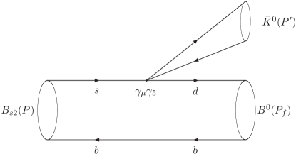
Figure 1: Strong decay of $B_{s2}\to B^{0}\bar{K}^{0}$

II Instantaneous Bethe-Salpeter Equation

In this section, we briefly review the Bethe-Salpeter equation and its instantaneous one, the Salpeter equation, and we introduce our notations.

The Bethe-Salpeter (BS) equation is read as BS :

$$(\not\!{p_{1}}-m_{1})\chi(q)(\not\!{p_{2}}+m_{2})=i\int\frac{d^{4}k}{(2\pi)^{4}}V(P,k,q)\chi(k)\;,$$ (1)

where $\chi(q)$ is the BS wave function, $V(P,k,q)$ is the interaction kernel between the quark and anti-quark, and $p_{1},p_{2}$ are the momentum of the quark 1 and anti-quark 2. The total momentum $P$ and the relative momentum $q$ are defined as:

$$p_{1}={\alpha}_{1}P+q,\;\;{\alpha}_{1}=\frac{m_{1}}{m_{1}+m_{2}}~{},$$

$$p_{2}={\alpha}_{2}P-q,\;\;{\alpha}_{2}=\frac{m_{2}}{m_{1}+m_{2}}~{}.$$

We divide the relative momentum $q$ into two parts, $q_{\parallel}$ and $q_{\perp}$,

$$q^{\mu}=q^{\mu}_{\parallel}+q^{\mu}_{\perp}\;,$$

$$q^{\mu}_{\parallel}\equiv(P\cdot q/M^{2})P^{\mu}\;,\;\;\;q^{\mu}_{\perp}\equiv q^{\mu}-q^{\mu}_{\parallel}\;.$$

Correspondingly, we have two Lorentz invariant variables:

$q_{p}=\frac{(P\cdot q)}{M}\;,\;\;\;\;\;q_{{}_{T}}=\sqrt{q^{2}_{p}-q^{2}}=\sqrt{-q^{2}_{\perp}}\;.$

When $\stackrel{{\scriptstyle\rightarrow}}{{P}}=0$, they turn to the usual component $q_{0}$ and $|\vec{q}|$, respectively.

In instantaneous approach, the kernel $V(P,k,q)$ takes the simple form Salp :

$$V(P,k,q)\Rightarrow V(k_{\perp},q_{\perp})\;.$$

Let us introduce the notations $\varphi_{p}(q^{\mu}_{\perp})$ and $\eta(q^{\mu}_{\perp})$ for three dimensional wave function as follows:

$$\varphi_{p}(q^{\mu}_{\perp})\equiv i\int\frac{dq_{p}}{2\pi}\chi(q^{\mu}_{\parallel},q^{\mu}_{\perp})\;,$$

$$\eta(q^{\mu}_{\perp})\equiv\int\frac{dk_{\perp}}{(2\pi)^{3}}V(k_{\perp},q_{\perp})\varphi_{p}(k^{\mu}_{\perp})\;.$$ (2)

Then the BS equation can be rewritten as:

$$\chi(q_{\parallel},q_{\perp})=S_{1}(p_{1})\eta(q_{\perp})S_{2}(p_{2})\;.$$ (3)

The propagators of the two constituents can be decomposed as:

$$S_{i}(p_{i})=\frac{\Lambda^{+}_{ip}(q_{\perp})}{J(i)q_{p}+\alpha_{i}M-\omega_{i}+i\epsilon}+\frac{\Lambda^{-}_{ip}(q_{\perp})}{J(i)q_{p}+\alpha_{i}M+\omega_{i}-i\epsilon}\;,$$ (4)

with

$$\omega_{i}=\sqrt{m_{i}^{2}+q^{2}_{{}_{T}}}\;,\;\;\;\Lambda^{\pm}_{ip}(q_{\perp})=\frac{1}{2\omega_{ip}}\left[\frac{\not\!{P}}{M}\omega_{i}\pm J(i)(m_{i}+{\not\!q}_{\perp})\right]\;,$$ (5)

where $i=1,2$ for quark and anti-quark, respectively, and $J(i)=(-1)^{i+1}$. Here $\Lambda^{\pm}_{ip}(q_{\perp})$ satisfy the relations:

$$\Lambda^{+}_{ip}(q_{\perp})+\Lambda^{-}_{ip}(q_{\perp})=\frac{\not\!{P}}{M}~{},\;\;\Lambda^{\pm}_{ip}(q_{\perp})\frac{\not\!{P}}{M}\Lambda^{\pm}_{ip}(q_{\perp})=\Lambda^{\pm}_{ip}(q_{\perp})~{},\;\;\Lambda^{\pm}_{ip}(q_{\perp})\frac{\not\!{P}}{M}\Lambda^{\mp}_{ip}(q_{\perp})=0~{}.$$ (6)

Introducing the notations $\varphi^{\pm\pm}_{p}(q_{\perp})$ as:

$$\varphi^{\pm\pm}_{p}(q_{\perp})\equiv\Lambda^{\pm}_{1p}(q_{\perp})\frac{\not\!{P}}{M}\varphi_{p}(q_{\perp})\frac{\not\!{P}}{M}\Lambda^{{\pm}}_{2p}(q_{\perp})\;,$$ (7)

and we have

$$\varphi_{p}(q_{\perp})=\varphi^{++}_{p}(q_{\perp})+\varphi^{+-}_{p}(q_{\perp})+\varphi^{-+}_{p}(q_{\perp})+\varphi^{--}_{p}(q_{\perp}).$$

Using contour integration over $q_{p}$ on both sides of Eq. (3), we obtain:

$$\varphi_{p}(q_{\perp})=\frac{\Lambda^{+}_{1p}(q_{\perp})\eta_{p}(q_{\perp})\Lambda^{+}_{2p}(q_{\perp})}{(M-\omega_{1}-\omega_{2})}-\frac{\Lambda^{-}_{1p}(q_{\perp})\eta_{p}(q_{\perp})\Lambda^{-}_{2p}(q_{\perp})}{(M+\omega_{1}+\omega_{2})}\;,$$

and the full Salpeter equation:

$$(M-\omega_{1}-\omega_{2})\varphi^{++}_{p}(q_{\perp})=\Lambda^{+}_{1p}(q_{\perp})\eta_{p}(q_{\perp})\Lambda^{+}_{2p}(q_{\perp})\;,$$

$$(M+\omega_{1}+\omega_{2})\varphi^{--}_{p}(q_{\perp})=-\Lambda^{-}_{1p}(q_{\perp})\eta_{p}(q_{\perp})\Lambda^{-}_{2p}(q_{\perp})\;,$$

$$\varphi^{+-}_{p}(q_{\perp})=\varphi^{-+}_{p}(q_{\perp})=0\;.$$ (8)

For the different $J^{PC}$ states, we give the general form of the wave functions (we will talk about them in Sec. III). Using the last two equations in Eq. (8), we can reduce the wave functions, then solve the wave functions by the first and second equations in Eq. (8) to get the wave functions and mass spectrum. We have discussed the solution of the Salpeter equation in detail in Refs. mass ; w1 .

The normalization condition for BS wave function is:

$$\int\frac{q_{{}_{T}}^{2}dq_{{}_{T}}}{2{\pi}^{2}}Tr\left[\overline{\varphi}^{++}\frac{{/}\!\!\!{P}}{M}\varphi^{++}\frac{{/}\!\!\!{P}}{M}-\overline{\varphi}^{--}\frac{{/}\!\!\!{P}}{M}\varphi^{--}\frac{{/}\!\!\!{P}}{M}\right]=2P_{0}\;.$$ (9)

In our model, Cornell potential, a linear scalar interaction plus a vector interaction is chosen as the instantaneous interaction kernel $V$:

$$V(r)=V_{s}(r)+V_{0}+\gamma_{{}_{0}}\otimes\gamma^{0}V_{v}(r)=\lambda r+V_{0}-\gamma_{{}_{0}}\otimes\gamma^{0}\frac{4}{3}\frac{\alpha_{s}}{r}~{},$$ (10)

where $\lambda$ is the string constant and $\alpha_{s}(\vec{q})$ is the running coupling constant. In order to fit the data of heavy quarkonia, a constant $V_{0}$ is often added to the scalar confining potential. We see that $V_{v}(r)$ diverges at $r=0$, in order to avoid the divergence, a factor $e^{-\alpha r}$ is added:

$$V_{s}(r)=\frac{\lambda}{\alpha}(1-e^{-\alpha r})~{},~{}~{}V_{v}(r)=-\frac{4}{3}\frac{\alpha_{s}}{r}e^{-\alpha r}~{}.$$ (11)

It is easy to show that when $\alpha r\ll 1$, the potential becomes the original one. In the momentum space and the rest frame of the bound state, the potential reads:

$$V(\vec{q})=V_{s}(\vec{q})+\gamma_{{}_{0}}\otimes\gamma^{0}V_{v}(\vec{q})~{},$$

$$V_{s}(\vec{q})=-(\frac{\lambda}{\alpha}+V_{0})\delta^{3}(\vec{q})+\frac{\lambda}{\pi^{2}}\frac{1}{{(\vec{q}}^{2}+{\alpha}^{2})^{2}}~{},~{}~{}V_{v}(\vec{q})=-\frac{2}{3{\pi}^{2}}\frac{\alpha_{s}(\vec{q})}{{(\vec{q}}^{2}+{\alpha}^{2})}~{},$$ (12)

where the running coupling constant $\alpha_{s}(\vec{q})$ is chosen as:

$$\alpha_{s}(\vec{q})=\frac{12\pi}{33-2N_{f}}\frac{1}{\log(a+\frac{{\vec{q}}^{2}}{\Lambda^{2}_{QCD}})}~{}.$$

With this equation and parameters shown in Sec. VI, one can find that $\alpha_{s}(m_{c})\simeq 0.38$ ($N_{f}=3$), $\alpha_{s}(m_{b})\simeq 0.26$ ($N_{f}=4$), and $N_{f}=3$ is chosen for $\bar{b}q$ system in this Letter. The constants $\lambda$, $\alpha$, $V_{0}$ and $\Lambda_{QCD}$ are the parameters that characterize the potential.

III Relativistic Wave Functions

In this section, by analyzing the parity and possible charge conjugation parity of corresponding bound states, we give the formulas of the wave functions that are in relativistic forms with definite parity and possible charge conjugation parity symmetry.

III.1 Wave Function for ${}^{1}S_{0}$ ($0^{-}$) state

The general form for the relativistic wave function of a pseudoscalar meson with the quantum number $J^{P}=0^{-}$ (or $J^{PC}=0^{-+}$ for an equal-mass system, a $q\bar{q}$ quarkonium) can be generally written as eight terms, which are constructed by $P,\ q_{{}_{P_{\bot}}}$ and gamma matrices, because of the instantaneous approximation, four terms with $P\cdot q_{{}_{P_{\bot}}}$ become zero, the general form for the relativistic Salpeter wave function of a pseudoscalar state $J^{P}=0^{-}$ (or $J^{PC}=0^{-+}$) can be written as w1 :

$$\varphi_{0^{-}}(q_{{}_{P_{\bot}}}) = \Big{[}f_{1}(q_{{}_{P_{\bot}}}){\not\!P}+f_{2}(q_{{}_{P_{\bot}}})M+f_{3}(q_{{}_{P_{\bot}}})\not\!{q_{{}_{P_{\bot}}}}+f_{4}(q_{{}_{P_{\bot}}})\frac{{\not\!P}\not\!{q_{{}_{P_{\bot}}}}}{M}\Big{]}\gamma_{5},$$ (13)

where $M$ is the mass of the pseudoscalar meson, and $f_{i}(q_{{}_{P_{\bot}}})$ are functions of $-q^{2}_{{}_{P_{\bot}}}$. Due to the last two equations of Eq. (8): $\varphi_{0^{-}}^{+-}=\varphi_{0^{-}}^{-+}=0$, we have:

$$f_{3}(q_{{}_{P_{\bot}}}) = \frac{f_{2}(q_{{}_{P_{\bot}}})M(-\omega_{1}+\omega_{2})}{m_{2}\omega_{1}+m_{1}\omega_{2}},~{}~{}~{}f_{4}(q_{{}_{P_{\bot}}})=-\frac{f_{1}(q_{{}_{P_{\bot}}})M(\omega_{1}+\omega_{2})}{m_{2}\omega_{1}+m_{1}\omega_{2}}.$$ (14)

Then there are only two independent unknown wave functions $f_{1}(q_{{}_{P_{\bot}}})$ and $f_{2}(q_{{}_{P_{\bot}}})$ in Eq. (13):

$$\varphi_{0^{-}}(q_{{}_{P_{\bot}}}) = \Big{[}f_{1}(q_{{}_{P_{\bot}}}){\not\!P}+f_{2}(q_{{}_{P_{\bot}}})M-f_{2}(q_{{}_{P_{\bot}}}){\not\!{q_{{}_{P_{\bot}}}}}\frac{M(\omega_{1}-\omega_{2})}{m_{2}\omega_{1}+m_{1}\omega_{2}}$$ (15)

$$+f_{1}(q_{{}_{P_{\bot}}}){\not\!{q_{{}_{P_{\bot}}}}\not\!P}\frac{\omega_{1}+\omega_{2}}{m_{2}\omega_{1}+m_{1}\omega_{2}}\Big{]}\gamma_{5}.$$

The numerical values of radial wave functions $f_{1}$, $f_{2}$ and eigenvalue $M$ can be obtained by solving the first two equations of Salpeter Eq. (8).

One can check that in Eq. (13), which we wrote as the wave function for $J^{P}=0^{-}$ (or $J^{PC}=0^{-+}$) state, all the terms except the one with $f_{3}$ have positive charge conjugate parity, while $f_{3}$ term has negative charge conjugate parity. When we consider the constraint relations, for equal mass system, $\omega_{1}=\omega_{2}$, so $f_{3}=0$ (Eq. (14)), then the whole wave function has positive charge conjugate parity, that is $0^{-+}$ state.

In our calculation, we obtain the numerical values of wave functions in the center-of-mass system of the bound state, so $q_{\parallel}$ and $q_{\perp}$ turn into the usual components $(q_{0},{\vec{0}})$ and $(0,{\vec{q}})$, $\omega_{1}=(m_{1}^{2}+{\vec{q}}^{2})^{1/2}$ and $\omega_{2}=(m_{2}^{2}+{\vec{q}}^{2})^{1/2}$. Then the normalization condition reads:

$$\displaystyle\int\frac{d\vec{q}}{(2\pi)^{3}}4f_{1}f_{2}M^{2}\Big{\{}\frac{m_{1}+m_{2}}{\omega_{1}+\omega_{2}}+\frac{\omega_{1}+\omega_{2}}{m_{1}+m_{2}}\displaystyle+\frac{2\vec{q}^{2}(m_{1}\omega_{1}+m_{2}\omega_{2})}{(m_{2}\omega_{1}+m_{1}\omega_{2})^{2}}\Big{\}}=2M.$$ (16)

The numerical values of the right sides of the first two equations in Eq. (8) are comparable, but since $M-\omega_{1}-\omega_{2}\ll M+\omega_{1}+\omega_{2}$ for bound state, we know that the numerical value of ${\varphi}^{++}(\vec{q})$ is much larger than that of ${\varphi}^{--}(\vec{q})$. So in the past, authors made a further approximation of the Salpeter equation, deleting the others in Eq. (8) except the first equation which is about the positive wave function ${\varphi}^{++}(\vec{q})$. This seems a reasonable approximation since ${\varphi}^{++}(\vec{q})$ is dominant, but we point out that, we can delete the term of ${\varphi}^{--}(\vec{q})$, but that should be done after we solve the full Salpeter equation, otherwise we obtain a non-relativistic wave function, not a relativistic one. Since with the further approximation, only one equation is left, then only one unknown $f_{i}$ wave function can be solved, we have to choose $f_{3}=f_{4}=0$, and $f_{1}=f_{2}$ in Eq. (13), then the wave function Eq. (13) becomes $\varphi_{0^{-}}=f_{1}({\not\!P}+M)\gamma_{5}$, this is well known Schrodinger wave function for a pseudoscalar. So in our calculation, we solve the full Salpeter equations Eq. (8), not only the first one in Eq. (8).

According to the Eq. (7) the relativistic positive wave function of pseudoscalar ${}^{1}S_{0}$ state ($B$ or $B_{s}$ in this Letter) in the center of mass system can be written as w1 :

$${\varphi}^{++}_{0^{-}}(\vec{q})=b_{1}\left[b_{2}+\frac{\not\!{P}}{M}+b_{3}\not\!{q_{\bot}}+b_{4}\frac{\not\!{q_{\bot}}\not\!{P}}{M}\right]{\gamma}_{5},$$ (17)

where the $b_{i}$ ($i=1,~{}2,~{}3,~{}4$) are related to the original radial wave function $f_{i}$, quark mass $m_{i}$, quark energy $w_{i}$ ($i=1,~{}2$) and meson mass $M$:

$$b_{1}=\frac{M}{2}\left({f}_{1}(\vec{q})+{f}_{2}(\vec{q})\frac{m_{1}+m_{2}}{w_{1}+w_{2}}\right),b_{2}=\frac{w_{1}+w_{2}}{m_{1}+m_{2}},b_{3}=-\frac{(m_{1}-m_{2})}{m_{1}w_{2}+m_{2}w_{1}},b_{4}=\frac{(w_{1}+w_{2})}{(m_{1}w_{2}+m_{2}w_{1})}.$$

Inserting the expressions of ${\varphi}^{++}_{0^{-}}(\vec{q})$ in Eq. (17) and corresponding ${\varphi}^{--}_{0^{-}}(\vec{q})$ (which can be easily obtained by ${\varphi}^{--}_{0^{-}}={\varphi}_{0^{-}}-{\varphi}^{++}_{0^{-}}$) into the first two equations of Eq. (8), we get two coupled integral equations (the explicit expressions can be found in Eqs. (24-25) in Ref. w1 ). By solving them, we obtained the numerical values of wave functions $f_{1}$, $f_{2}$ and eigenvalue $M$.

III.2 Wave Function for ${}^{3}S_{1}$ ($1^{-}$) state

Because of the instantaneous approximation, instead of 16 terms, the general form for the relativistic wave function of vector state $J^{P}=1^{-}$ (or $J^{PC}=1^{--}$ for quarkonium) can be written as eight terms, which are constructed by $P$, $q$, $\varepsilon$ and gamma matrices glwang :

$$\varphi_{1^{-}}(q_{\perp})=q_{\perp}\cdot{\varepsilon}^{(\lambda)}\left[f_{1}(q_{\perp})+\frac{\not\!P}{M}f_{2}(q_{\perp})+\frac{{\not\!q}_{\perp}}{M}f_{3}(q_{\perp})+\frac{{\not\!P}{\not\!q}_{\perp}}{M^{2}}f_{4}(q_{\perp})\right]+M{\not\!\varepsilon}^{(\lambda)}f_{5}(q_{\perp})$$

$$+{\not\!\varepsilon}^{(\lambda)}{\not\!P}f_{6}(q_{\perp})+({\not\!q}_{\perp}{\not\!\varepsilon}^{(\lambda)}-q_{\perp}\cdot{\varepsilon}^{(\lambda)})f_{7}(q_{\perp})+\frac{1}{M}({\not\!P}{\not\!\varepsilon}^{(\lambda)}{\not\!q}_{\perp}-{\not\!P}q_{\perp}\cdot{\varepsilon}^{(\lambda)})f_{8}(q_{\perp}),$$ (18)

where ${\varepsilon}^{(\lambda)}$ is the polarization vector of the vector meson. One should note that we use the same notations of the radial wave functions $f_{i}$ for pseudoscalar and vector mesons, but they are different. It should be indicated that we will use them for other states (see below), but we remind the readers that their numerical values are different for the different states.

The equations $\varphi^{+-}_{1^{-}}(q_{\perp})=\varphi^{-+}_{1^{-}}(q_{\perp})=0\;$ give the constraints on the components of the wave function $\varphi_{1^{-}}(q_{\perp})$, so we have the relations

$$f_{1}(q_{\perp})=\frac{\left[q_{\perp}^{2}f_{3}(q_{\perp})+M^{2}f_{5}(q_{\perp})\right](m_{1}m_{2}-\omega_{1}\omega_{2}+q_{\perp}^{2})}{M(m_{1}+m_{2})q_{\perp}^{2}},~{}~{}~{}f_{7}(q_{\perp})=\frac{f_{5}(q_{\perp})M(-\omega_{1}+\omega_{2})}{(m_{1}\omega_{2}+m_{2}\omega_{1})},$$

$$f_{2}(q_{\perp})=\frac{\left[-q_{\perp}^{2}f_{4}(q_{\perp})+M^{2}f_{6}(q_{\perp})\right](m_{1}\omega_{2}-m_{2}\omega_{1})}{M(\omega_{1}+\omega_{2})q_{\perp}^{2}},~{}~{}~{}f_{8}(q_{\perp})=\frac{f_{6}(q_{\perp})M(\omega_{1}\omega_{2}-m_{1}m_{2}-q_{\perp}^{2})}{(m_{1}+m_{2})q_{\perp}^{2}}.$$

Then there are only four independent wave functions $f_{3}(q_{\perp})$, $f_{4}(q_{\perp})$, $f_{5}(q_{\perp})$ and $f_{6}(q_{\perp})$ in Eq. (18).

One can check that in Eq. (18), all the terms except those with $f_{2}$ and $f_{7}$ are negative under charge conjugation operation, while the terms with $f_{2}$ and $f_{7}$ are positive. Applying the constraint relations, for equal mass system, we found the terms with $f_{2}$ and $f_{7}$ disappear, then the whole wave function has negative charge conjugate parity, that is $1^{--}$ state. The similar relations hold for the following $P$ wave states, so we will not show the details again.

Wave functions $f_{3}({\vec{q}})$, $f_{4}({\vec{q}})$, $f_{5}({\vec{q}})$ and $f_{6}({\vec{q}})$ will fulfill the normalization condition:

$$\int\frac{d{\vec{q}}}{(2\pi)^{3}}\frac{16\omega_{1}\omega_{2}}{3}\left\{3f_{5}f_{6}\frac{M^{2}}{m_{1}\omega_{2}+m_{2}\omega_{1}}+\frac{\omega_{1}\omega_{2}-m_{1}m_{2}+{\vec{q}}^{2}}{(m_{1}+m_{2})(\omega_{1}+\omega_{2})}\left[f_{4}f_{5}-f_{3}\left(f_{4}\frac{{\vec{q}}^{2}}{M^{2}}+f_{6}\right)\right]\right\}=2M.$$ (19)

The relativistic positive wave function of ${}^{3}S_{1}$ state ($B^{*}$ or $B_{s}^{*}$ in this Letter) can be written as:

$${\varphi}_{1^{-}}^{++}(\vec{q}) = b_{1}\not\!{\varepsilon}^{(\lambda)}+b_{2}\not\!{\varepsilon}^{(\lambda)}\not\!{P}+b_{3}(\not\!{q_{\bot}}\not\!{\varepsilon}^{(\lambda)}-q_{\bot}\cdot{\varepsilon}^{(\lambda)})+b_{4}(\not\!{P}\not\!{\varepsilon}^{(\lambda)}\not\!{q_{\bot}}-\not\!{P}q_{\bot}\cdot{\varepsilon}^{(\lambda)})$$ (20)

$$+q_{\bot}\cdot{\varepsilon}^{(\lambda)}(b_{5}+b_{6}\not\!{P}+b_{7}\not\!{q_{\bot}}+b_{8}\not\!{q_{\bot}}\not\!{P}),$$

where we first defined the parameters $n_{i}$ which are functions of $f_{i}$ (${}^{3}S_{1}$ wave functions):

$$n_{1}={f}_{5}(\vec{q})-{f}_{6}(\vec{q})\frac{(w_{1}+w_{2})}{(m_{1}+m_{2})},n_{2}={f}_{5}(\vec{q})-{f}_{6}(\vec{q})\frac{(m_{1}+m_{2})}{(w_{1}+w_{2})},n_{3}={f}_{3}(\vec{q})+{f}_{4}(\vec{q})\frac{(m_{1}+m_{2})}{(w_{1}+w_{2})},$$

then we defined the parameters $b_{i}$ which are functions of $f_{i}$ and $n_{i}$:

$$b_{1}=\frac{M}{2}n_{1},b_{2}=-\frac{M}{2}\frac{(m_{1}+m_{2})}{(w_{1}+w_{2})}n_{1},b_{3}=\frac{M}{2}\frac{(w_{2}-w_{1})}{(m_{1}w_{2}+m_{2}w_{1})}n_{1},b_{4}=\frac{1}{2}\frac{(w_{1}+w_{2})}{(w_{1}w_{2}+m_{1}m_{2}-{q_{\bot}^{2}})}n_{1},$$

$$b_{5}=\frac{1}{2M}\frac{m_{1}+m_{2}}{(w_{1}w_{2}+m_{1}m_{2}+{q_{\bot}^{2}})}(M^{2}n_{2}+{q_{\bot}^{2}}n_{3}),b_{6}=\frac{1}{2M^{2}}\frac{w_{1}-w_{2}}{(w_{1}w_{2}+m_{1}m_{2}+{q_{\bot}^{2}})}(M^{2}n_{2}+{q_{\bot}^{2}}n_{3}),$$

$$b_{7}=\frac{n_{3}}{2M}-\frac{f_{6}(\vec{q})M}{(m_{1}w_{2}+m_{2}w_{1})},b_{8}=\frac{1}{2M^{2}}\frac{w_{1}+w_{2}}{m_{1}+m_{2}}n_{3}-f_{5}(\vec{q})\frac{w_{1}+w_{2}}{(m_{1}+m_{2})(w_{1}w_{2}+m_{1}m_{2}-{q_{\bot}^{2}})}.$$

Similar to the method in last subsection, where we obtained the wave functions and eigenvalues for pseudoscalar states, inserting ${\varphi}_{1^{-}}^{++}(\vec{q})$ and corresponding ${\varphi}_{1^{-}}^{--}(\vec{q})$ into the first two equations of Eq. (8), we obtained four independent coupled integral equations (Eqs. (37-40) in Ref. mass ), by solving them, we obtained the numerical results of mass spectra and wave functions. For other states, see below, we will not show the details of how to solve them, interested reader can find the details elsewhere, for example, in Ref. mass .

One should also note that we cite same notations of $m_{i}$, $w_{i}$, $M$, $P$, and $b_{i}$ as used in last subsection for pseudoscalar meson, but they are different for different states. And we also use the same notations for other mesons, like the following $P$ wave states.

III.3 Wave function for ${}^{3}P_{0}$ state

The general form for the relativistic Salpeter wave function of ${}^{3}P_{0}$ state, which $J^{P}=0^{+}$ (or $J^{PC}=0^{++}$ for equal mass system), can be written as w2 :

$$\varphi_{0^{+}}(q_{\perp})=f_{1}(q_{\perp}){\not\!q}+f_{2}(q_{\perp})\frac{{\not\!P}{\not\!q}_{\perp}}{M}+f_{3}(q_{\perp})M+f_{4}(q_{\perp}){\not\!P}.$$ (21)

The equations $\varphi^{+-}_{0^{+}}(q_{\perp})=\varphi^{-+}_{0^{+}}(q_{\perp})=0\;$ give the constraints on the components of the wave functions, so we have the relations

$$f_{3}(q_{\perp})=\frac{f_{1}(q_{\perp})q_{\perp}^{2}(m_{1}+m_{2})}{M(\omega_{1}\omega_{2}+m_{1}m_{2}+q_{\perp}^{2})},~{}~{}~{}f_{4}(q_{\perp})=\frac{f_{2}(q_{\perp})q_{\perp}^{2}(\omega_{1}-\omega_{2})}{M(m_{1}\omega_{2}+m_{2}\omega_{1})}.$$

Then there are only two independent wave functions $f_{1}(q_{\perp})$ and $f_{2}(q_{\perp})$. From Eq. (8), we obtain two coupled integral equations, by solving them, we obtain the numerical results of mass spectra and wave functions.

The normalization condition for the ${}^{3}P_{0}$ wave function is:

$$\int\frac{d{\vec{q}}}{(2\pi)^{3}}\frac{16f_{1}f_{2}\omega_{1}\omega_{2}{\vec{q}}^{2}}{m_{1}\omega_{2}+m_{2}\omega_{1}}=2M.$$ (22)

The relativistic positive energy wave function of $B_{s0}~{}(^{3}P_{0})$ can be written as:

$${\varphi}_{0^{+}}^{++}(\vec{q})=a_{1}(\not\!{q_{\bot}}+a_{2}\frac{\not\!{P}\not\!{q_{\bot}}}{M}+a_{3}+a_{4}\frac{\not\!{P}}{M}),$$ (23)

where the parameters $a_{i}$ are functions of $f_{1}$ and $f_{2}$ ($0^{+}$ wave function) and are defined as:

$$a_{1}=\frac{1}{2}\left({f}_{1}(\vec{q})+{f}_{2}(\vec{q})\frac{m_{1}+m_{2}}{w_{1}+w_{2}}\right),a_{2}=\frac{w_{1}+w_{2}}{m_{1}+m_{2}},a_{3}=q_{\bot}^{2}\frac{(w_{1}+w_{2})}{m_{1}w_{2}+m_{2}w_{1}},a_{4}=\frac{(m_{2}w_{1}-m_{1}w_{2})}{(m_{1}+m_{2})}.$$

III.4 Wave function for ${}^{3}P_{1}$ state

The general form for the Salpeter wave function of ${}^{3}P_{1}$ state, which $J^{P}=1^{+}$ (or $J^{PC}=1^{++}$ for equal mass system), can be written as w2 :

$$\varphi_{{}^{3}P_{1}}(q_{\perp})=i\epsilon_{\mu\nu\alpha\beta}P^{\nu}q_{\perp}^{\alpha}\varepsilon^{\beta}\left[f_{1}M\gamma^{\mu}+f_{2}{\not\!P}\gamma^{\mu}+f_{3}{\not\!q}_{\perp}\gamma^{\mu}+if_{4}\epsilon^{\mu\rho\sigma\delta}q_{\perp\rho}P_{\sigma}\gamma_{\delta}\gamma_{5}/M\right]/M^{2},$$ (24)

where ${\varepsilon}^{(\lambda)}$ is the polarization vector of the ${}^{3}P_{1}$ state.

The constraint equations give us the relations:

$$f_{3}(q_{\perp})=\frac{f_{1}(q_{\perp})M(m_{1}\omega_{2}-m_{2}\omega_{1})}{q_{\perp}^{2}(\omega_{1}+\omega_{2})},~{}~{}~{}f_{4}(q_{\perp})=\frac{f_{2}(q_{\perp})M(-\omega_{1}\omega_{2}+m_{1}m_{2}+q_{\perp}^{2})}{q_{\perp}^{2}(m_{1}+m_{2})}.$$

The normalization condition for the ${}^{3}P_{1}$ wave function is:

$$\int\frac{d{\vec{q}}}{(2\pi)^{3}}\frac{32f_{1}f_{2}\omega_{1}\omega_{2}(\omega_{1}\omega_{2}-m_{1}m_{2}+{\vec{q}}^{2})}{3(m_{1}+m_{2})(\omega_{1}+\omega_{2})}=2M.$$ (25)

The relativistic positive energy wave function of ${}^{3}P_{1}$ state can be written as:

$${\varphi}_{{}^{3}P_{1}}^{++}(\vec{q})=i{\epsilon}_{\mu\nu\alpha\beta}P^{\nu}q^{\alpha}_{\bot}{\varepsilon}^{\beta(\lambda)}a_{1}[M{\gamma}^{\mu}+a_{2}{\gamma}^{\mu}\not\!{P}+a_{3}{\gamma}^{\mu}\not\!{q_{\bot}}+a_{4}{\gamma}^{\mu}\not\!{P}\not\!{q_{\bot}}]/M^{2},$$ (26)

where the parameters $a_{i}$ are functions of $f_{1}$ and $f_{2}$ (${}^{3}P_{1}$ wave function) and are defined as:

$$a_{1}=\frac{1}{2}\left(f_{1}(\vec{q})+f_{2}(\vec{q})\frac{w_{1}+w_{2}}{m_{1}+m_{2}}\right),a_{2}=-\frac{m_{1}+m_{2}}{w_{1}+w_{2}},a_{3}=\frac{M(w_{1}-w_{2})}{m_{1}w_{2}+m_{2}w_{1}},a_{4}=-\frac{(m_{1}+m_{2})}{m_{1}w_{2}+m_{2}w_{1}}.$$

III.5 Wave function for ${}^{1}P_{1}$ state

The general form for the Salpeter wave function of ${}^{1}P_{1}$ state, which $J^{P}=1^{+}$ (or $J^{PC}=1^{+-}$ for equal mass system), can be written as w2 :

$$\varphi_{{}^{1}P_{1}}(q_{\perp})=q_{\perp}\cdot{\varepsilon^{(\lambda)}}\left[f_{1}(q_{\perp})+f_{2}(q_{\perp})\frac{{\not\!P}}{M}+f_{3}(q_{\perp})\frac{{\not\!q_{\perp}}}{M}+f_{4}(q_{\perp})\frac{\not\!{P}{\not\!q}}{M^{2}}\right]\gamma_{5},$$ (27)

where ${\varepsilon^{(\lambda)}}$ is the polarization vector of the ${}^{1}P_{1}$ state.

The constraint equations provide us the relations:

$$f_{3}(q_{\perp})=-\frac{f_{1}(q_{\perp})M(m_{1}-m_{2})}{(\omega_{1}\omega_{2}+m_{1}m_{2}-q_{\perp}^{2})},~{}~{}~{}f_{4}(q_{\perp})=-\frac{f_{2}(q_{\perp})M(\omega_{1}+\omega_{2})}{(m_{1}\omega_{2}+m_{2}\omega_{1})}.$$

The normalization condition for the ${}^{1}P_{1}$ wave function is:

$$\int\frac{d{\vec{q}}}{(2\pi)^{3}}\frac{16f_{1}f_{2}\omega_{1}\omega_{2}{\vec{q}}^{2}}{3(m_{1}\omega_{2}+m_{2}\omega_{1})}=2M.$$ (28)

The relativistic positive energy wave function of ${}^{1}P_{1}$ can be written as:

$${\varphi}_{{}^{1}P_{1}}^{++}(\vec{q})=(\varepsilon^{(\lambda)}\cdot q_{\bot})a_{1}\left[1+a_{2}\frac{\not\!P}{M}+a_{3}\not\!{q_{\bot}}+a_{4}\frac{\not\!{q_{\bot}}\not\!P}{M}\right]{\gamma}_{5},$$ (29)

where the parameters $a_{i}$ are functions of $f_{1}$ and $f_{2}$ (${}^{1}P_{1}$ wave function) and are defined as:

$$a_{1}=\frac{1}{2}\left(f_{1}(\vec{q}+f_{2}(\vec{q})\frac{w_{1}+w_{2}}{m_{1}+m_{2}})\right),a_{2}=\frac{m_{1}+m_{2}}{w_{1}+w_{2}},a_{3}=-\frac{w_{1}-w_{2}}{m_{2}w_{1}+m_{1}w_{2}},a_{4}=\frac{m_{1}+m_{2}}{m_{2}w_{1}+m_{1}w_{2}}.$$

The wave functions of two physical $1^{+}$ states (or ${\frac{1}{2}}^{+}$ and ${\frac{3}{2}}^{+}$) are the mixing of ${\varphi}_{{}^{3}P_{1}}^{++}(\vec{q})$ and ${\varphi}_{{}^{1}P_{1}}^{++}(\vec{q})$, see Eq. (IV) below.

III.6 Wave function for ${}^{3}P_{2}$ state

The general form for the relativistic wave function of tensor $J^{P}=2^{+}$ state (or $J^{PC}=2^{++}$ for equal mass system) can be written as w3 :

$$\Psi_{2^{+}}(\vec{q})={\varepsilon}_{\mu\nu}^{(\lambda)}{q_{\perp}^{\nu}}\left\{{q_{\perp}^{\mu}}\left[f_{1}(\vec{q})+\frac{\not\!P}{M}f_{2}(\vec{q})+\frac{{\not\!q}_{\perp}}{M}f_{3}(\vec{q})+\frac{{\not\!P}{\not\!q}_{\perp}}{M^{2}}f_{4}(\vec{q})\right]\right.$$

$$\left.+{\gamma^{\mu}}\left[Mf_{5}(\vec{q})+{\not\!P}f_{6}(\vec{q})+{\not\!q}_{\perp}f_{7}(\vec{q})\right]+\frac{i}{M}f_{8}(\vec{q})\epsilon^{\mu\alpha\beta\gamma}P_{\alpha}q_{\perp\beta}\gamma_{\gamma}\gamma_{5}\right\},$$ (30)

where ${\varepsilon}_{\mu\nu}^{(\lambda)}$ is the polarization tensor of the $2^{+}$ state. The constraint equations give further relations:

$$f_{1}(\vec{q})=\frac{\left[q_{\perp}^{2}f_{3}(\vec{q})+M^{2}f_{5}(\vec{q})\right](\omega_{1}+\omega_{2})-M^{2}f_{5}(\vec{q})(\omega_{1}-\omega_{2})}{M(m_{1}\omega_{2}+m_{2}\omega_{1})},~{}$$

$$f_{2}(\vec{q})=\frac{\left[q_{\perp}^{2}f_{4}(\vec{q})-M^{2}f_{6}(\vec{q})\right](\omega_{1}-\omega_{2})}{M(m_{1}\omega_{2}+m_{2}\omega_{1})},~{}~{}$$

$$~{}~{}f_{7}(\vec{q})=\frac{f_{5}(\vec{q})M(\omega_{1}-\omega_{2})}{m_{1}\omega_{2}+m_{2}\omega_{1}},~{}~{}~{}~{}f_{8}(\vec{q})=\frac{f_{6}(\vec{q})M(\omega_{1}+\omega_{2})}{m_{1}\omega_{2}+m_{2}\omega_{1}}.$$ (31)

Only four independent wave functions $f_{3}(\vec{q})$, $f_{4}(\vec{q})$, $f_{5}(\vec{q})$ and $f_{6}(\vec{q})$, the numerical values and the bound state mass $M$ can be obtained by solving the full Salpeter equation.

These four independent wave functions fulfil the normalization condition:

$$\int\frac{d{\vec{q}}}{(2\pi)^{3}}\frac{16~{}\omega_{1}\omega_{2}~{}{\vec{q}}^{2}}{15(m_{1}\omega_{2}+m_{2}\omega_{1})}\left\{f_{5}~{}f_{6}~{}M^{2}\left[5+\frac{(m_{1}+m_{2})(m_{2}\omega_{1}-m_{1}\omega_{2})}{\omega_{1}\omega_{2}(\omega_{1}+\omega_{2})}\right]\right.$$

$$\left.+f_{4}~{}f_{5}~{}{\vec{q}}^{2}\left[2+\frac{(m_{1}+m_{2})(m_{2}\omega_{1}-m_{1}\omega_{2})}{\omega_{1}\omega_{2}(\omega_{1}+\omega_{2})}\right]-2~{}{\vec{q}}^{2}f_{3}\left(f_{4}\frac{{\vec{q}}^{2}}{M^{2}}+f_{6}\right)\right\}=2M.$$ (32)

The relativistic positive energy wave function of $B_{s2}~{}(^{3}P_{2})$ can be written as:

$${\varphi}^{++}_{{}^{3}P_{2}}={\varepsilon}^{(\lambda)}_{\mu\nu}q^{\nu}_{\bot}\{q^{\mu}_{\bot}[a_{1}+a_{2}\frac{\not\!P}{M}+a_{3}\frac{{\not\!q_{\bot}}}{M}+a_{4}\frac{\not\!q_{\bot}\not\!P}{M^{2}}]+{\gamma}^{\mu}[a_{5}+a_{6}\frac{\not\!P}{M}+a_{7}\frac{\not\!q_{\bot}}{M}+a_{8}\frac{\not\!P\not\!q_{\bot}}{M^{2}}]\},$$ (33)

similar to $1^{-}$ state, we first defined $n_{i}$ as:

$$n_{1}=f_{3}(\vec{q})+f_{4}(\vec{q})\frac{m_{1}+m_{2}}{w_{1}+w_{2}},~{}n_{2}=f_{5}(\vec{q})-f_{6}(\vec{q})\frac{w_{1}+w_{2}}{m_{1}+m_{2}},$$

then we defined the parameters $a_{i}$:

$$a_{1}=\frac{(w_{1}+w_{2})q^{2}_{\bot}}{2M(m_{1}w_{2}+m_{2}w_{1})}n_{1}+\frac{(f_{5}(\vec{q})w_{2}-f_{6}(\vec{q})m_{2})M}{m_{1}w_{2}+m_{2}w_{1}},$$

$$a_{2}=\frac{(m_{1}-m_{2})q^{2}_{\bot}}{2M(m_{1}w_{2}+m_{2}w_{1})}n_{1}+\frac{(f_{6}(\vec{q})w_{2}-f_{5}(\vec{q})m_{2})M}{m_{1}w_{2}+m_{2}w_{1}},$$

$$a_{3}=\frac{1}{2}n_{1}+\frac{f_{6}(\vec{q})M^{2}}{m_{1}w_{2}+m_{2}w_{1}},~{}a_{4}=\frac{1}{2}(-\frac{w_{1}+w_{2}}{m_{1}+m_{2}})n_{1}+\frac{f_{5}(\vec{q})M^{2}}{m_{1}w_{2}+m_{2}w_{1}},$$

$$a_{5}=\frac{M}{2}n_{2},~{}a_{6}=\frac{M(m_{1}+m_{2})}{2(w_{1}+w_{2})}n_{2},~{}a_{7}=\frac{M^{2}(w_{1}-w_{2})}{2(m_{2}w_{1}+m_{1}w_{2})}n_{2},~{}a_{8}=\frac{M^{2}(m_{1}+m_{2})}{2(m_{2}w_{1}+m_{1}w_{2})}n_{2}.$$

IV Transition Matrix Element

In this section, we show the method to formulate the transition matrix element, which is general for all the decay channels in this Letter.

Considering the limitations of phase spaces, there are seven dominant strong decay channels for $B^{*}_{sJ}$ states: $B_{s0}\to B^{0}_{s}\pi^{0}$, $B_{s0}\to B\bar{K}$, $B^{\prime}_{s1}\to B_{s}^{*0}\pi^{0}$, $B^{\prime}_{s1}\to B^{*}\bar{K}$, $B_{s1}\to B^{*}\bar{K}$, $B_{s2}\to B\bar{K}$ and $B_{s2}\to B^{*}\bar{K}$ (where $B\bar{K}=B^{+}K^{-}+B^{0}\bar{K^{0}}$ and $B^{*}\bar{K}=B^{*+}K^{-}+B^{*0}\bar{K^{0}}$). Since all the light mesons in final states are pseudoscalars, we can give a unique formulation of the transition matrix element for these seven decay channels. By using the reduction formula, PCAC relation and low energy theorem, taking the channel $B_{s2}\to B\bar{K}$ as an example, see Figure 1, the corresponding transition matrix element can be written as wang :

$$T(B_{s2}\to B^{0}\bar{K}^{0})=\frac{P^{\prime\mu}}{f_{{}_{K}}}<B^{0}(P_{f})|\bar{d}{\gamma}_{\mu}\gamma_{5}s|B_{s2}(P)>,$$ (34)

where $f_{{}_{K}}$ is the decay constant of pseudoscalar $K$ meson, $P^{\prime}$ is the momentum of $K$. The contribution of the light pseudoscalar is reduced to a factor $\frac{P^{\prime\mu}}{f_{{}_{K}}}$, then the main part of the calculation in Eq. (34) is to calculate the transition element $<B^{0}(P_{f})|\bar{d}{\gamma}_{\mu}\gamma_{5}s|B_{s2}(P)>$.

If we further choose the instantaneous approach, according to the Mandelstam formalism Mand , at the leading order, the transition matrix element can be written as an integral equation of the corresponding initial and final state wave functions w4 :

$$\langle B^{0}(P_{f})|\bar{d}{\gamma}_{\mu}\gamma_{5}s|B_{s2}(P)\rangle=\int\frac{d\vec{q}}{(2\pi)^{3}}Tr\Big{\{}\bar{\varphi}^{\prime++}_{B^{0}}(\vec{q^{\prime}}){\gamma}_{\mu}{\gamma}_{5}{\varphi}^{++}_{B_{s2}}(\vec{q})\frac{\not\!P}{M}\Big{\}}\,,$$ (35)

where $P$ and $M$ are the momentum and mass of initial state $B_{s2}$; $\vec{q}$ and $\vec{q^{\prime}}=\vec{q}+\frac{m_{b}}{m_{b}+m_{d}}\times\vec{P}_{f}$ are the relative momenta of quark and anti-quark in the initial state $B_{s2}$ and the final state $B^{0}$, respectively, which are defined as $\vec{q}=\vec{p}_{s}=-\vec{p}_{b}$ and $\vec{q^{\prime}}=\frac{m_{b}}{m_{b}+m_{d}}\times\vec{P}_{f}-\vec{p}_{b}$ in the center of mass system of initial state $B_{s2}$; ${\varphi}^{++}(q_{\bot})$ and $\bar{\varphi}^{\prime++}(q_{\bot}^{\prime})$ are the positive energy wave functions of $B_{s2}$ and $B^{0}$, which are given in last section.

In our model, improved B-S method, which is based on the constituent quark model, we give the forms of wave functions by considering the quantum number $J^{P}$ or $J^{PC}$ for different states, and these states in our model are labelled as ${}^{1}S_{0}$ ($0^{-}$ state), ${}^{3}S_{1}$ ($1^{-}$ state), ${}^{3}P_{J}$ ($J=1,~{}2,~{}3$) ($0^{+}$, $1^{+}$, $2^{+}$) and ${}^{1}P_{1}$ ($1^{+}$). For the unequal mass system, the ${}^{3}P_{1}$ and ${}^{1}P_{1}$ states are not physical states, the two physical states ${\frac{1}{2}}^{+}$ and ${\frac{3}{2}}^{+}$, which are the mixtures of them, can be expressed as rosner ; hqet ; aa ; wise :

$$|B^{\prime}_{s1}>=|{\frac{1}{2}}^{+}>=\sin\theta|^{1}P_{1}>-\cos\theta|^{3}P_{1}>,$$

$$|B_{s1}>=|{\frac{3}{2}}^{+}>=\cos\theta|^{1}P_{1}>+\sin\theta|^{3}P_{1}>,$$ (36)

where $\theta$ is the mixing angle and $\theta\approx 35.3^{\circ}$ in the heavy quark limit.

The strong decay amplitudes can be described by the strong coupling constants, they are defined as:

$$T(B_{s0}\to B_{s}\pi)=G_{B_{s0}B_{s}\pi},$$

$$T(B_{s0}\to B\bar{K})=G_{B_{s0}B\bar{K}},$$

$$T(B^{\prime}_{s1}\to B_{s}^{*}\pi)=G_{B^{\prime}_{s1}B_{s}^{*}\pi}({\varepsilon}_{1}^{(\lambda^{\prime})}\cdot v)({\varepsilon}^{(\lambda)}\cdot v^{\prime})+F_{B^{\prime}_{s1}B_{s}^{*}\pi}({\varepsilon}_{1}^{(\lambda^{\prime})}\cdot{\varepsilon}^{(\lambda)}),$$

$$T(B^{\prime}_{s1}\to B^{*}\bar{K})=G_{B^{\prime}_{s1}B^{*}\bar{K}}({\varepsilon}_{1}^{(\lambda^{\prime})}\cdot v)({\varepsilon}^{(\lambda)}\cdot v^{\prime})+F_{B^{\prime}_{s1}B^{*}\bar{K}}({\varepsilon}_{1}^{(\lambda^{\prime})}\cdot{\varepsilon}^{(\lambda)}),$$

$$T(B_{s1}\to B^{*}\bar{K})=G_{B_{s1}B^{*}\bar{K}}({\varepsilon}_{1}^{(\lambda^{\prime})}\cdot v)({\varepsilon}^{(\lambda)}\cdot v^{\prime})+F_{B_{s1}B^{*}\bar{K}}({\varepsilon}_{1}^{(\lambda^{\prime})}\cdot{\varepsilon}^{(\lambda)}),$$

$$T(B_{s2}\to B\bar{K})=G_{B_{s2}B\bar{K}}{\varepsilon}_{\mu\nu}^{(\lambda)}v^{\prime\mu}v^{\prime\nu},$$

$$T(B_{s2}\to B^{*}\bar{K})=iG_{B_{s2}B^{*}\bar{K}}{\varepsilon}_{\mu\nu}^{(\lambda)}v^{\prime\nu}{\epsilon}^{{\varepsilon}_{1}^{(\lambda^{\prime})}vv^{\prime}\mu},$$ (37)

where $G_{B_{s0}B_{s}\pi},\cdots G_{B_{s2}B^{*}\bar{K}}$ are the strong coupling constants; $v=\frac{P}{M}$ and $v^{\prime}=\frac{P_{f}}{M_{f}}$ are four-velocities of initial state and final state; ${\varepsilon}$ is the polarization vector of initial state $B^{\prime}_{s1}$ or $B_{s1}$, ${\varepsilon}_{1}$ is the polarization vector of final state $B_{s}^{*}$ or $B^{*}$, ${\varepsilon}_{\mu\nu}$ is the polarization vector of initial state $B_{s2}$; $P,~{}P_{f}$ are the four-momenta of initial and final heavy states, respectively.

V Decay Widths

The decay channels of $B_{s0}\to B\bar{K}$, $B^{\prime}_{s1}\to B^{*}\bar{K}$, $B_{s1}\to B^{*}\bar{K}$, $B_{s2}\to B\bar{K}$ and $B_{s2}\to B^{*}\bar{K}$ are OZI rule allowed, through the Eq. (34) and Eq. (35) the calculations of corresponding decay widths are straightforward:

$$\Gamma_{{B_{s0}B\bar{K}}}=\frac{|\vec{P}_{f}|}{8\pi M^{2}}\left|{T(B_{s0}\to B\bar{K})}\right|^{2},\ \ \ \Gamma_{{B^{\prime}_{s1}B^{*}\bar{K}}}=\frac{|\vec{P}_{f}|}{24\pi M^{2}}\sum_{\lambda,\lambda^{\prime}}\left|{T(B^{\prime}_{s1}\to B^{*}\bar{K})}\right|^{2},$$

$$\Gamma_{{B_{s1}B^{*}\bar{K}}}=\frac{|\vec{P}_{f}|}{24\pi M^{2}}\sum_{\lambda,\lambda^{\prime}}\left|T(B_{s1}\to B^{*}\bar{K})\right|^{2},\ \ \ \Gamma_{B_{s2}B\bar{K}}=\frac{|\vec{P}_{f}|}{40\pi M^{2}}\sum_{\lambda}\left|T(B_{s2}\to B\bar{K})\right|^{2},$$

$$\Gamma_{B_{s2}B^{*}\bar{K}}=\frac{|\vec{P}_{f}|}{40\pi M^{2}}\sum_{\lambda,\lambda^{\prime}}\left|T(B_{s2}\to B^{*}\bar{K})\right|^{2}.$$ (38)

The decays of $B_{s0}\to B_{s}\pi$ and $B^{\prime}_{s1}\to B_{s}^{*}\pi$ violate the isospin symmetry which only occur through $\pi^{0}-\eta$ mixing mix1 . According to Dashen’ theorem dashen , the decay widths can be written as:

$$\Gamma_{{B_{s0}B_{s}\pi}}=\frac{|\vec{P}_{f}|}{8\pi M^{2}}\left|\frac{T(B_{s0}\to B_{s}\pi)t_{\pi\eta}}{m^{2}_{\pi}-m^{2}_{\eta}}\right|^{2},\ \ \ \Gamma_{{B^{\prime}_{s1}B_{s}^{*}\pi}}=\frac{|\vec{P}_{f}|}{24\pi M^{2}}\sum_{\lambda,\lambda^{\prime}}\left|\frac{T(B^{\prime}_{s1}\to B_{s}^{*}\pi)t_{\pi\eta}}{m^{2}_{\pi}-m^{2}_{\eta}}\right|^{2},$$ (39)

where $t_{\pi\eta}=<\pi^{0}|\mathcal{H}|\eta>$ is the ${\pi}^{0}-\eta$ transition matrix, $m_{\pi}$ and $m_{\eta}$ are the masses of $\pi$ and $\eta$. The chosen value of $t_{\pi\eta}=-0.003$ GeV² dashen is very small, which result in narrow decay widths of these two channels.

VI Numerical Results and Discussions

In order to obtain the masses and wave functions of initial and final states, which are used to calculate the transition matrix elements and decay widths, we solve the instantaneous B-S equation BS ; Salp , and the parameters are chosen as: $a=e=2.7183,\lambda=0.21$ GeV², ${\Lambda}_{QCD}=0.27$ GeV, $\alpha=0.06$ GeV, $m_{b}=4.96$ GeV, $m_{s}=0.5$ GeV, $m_{u}=0.305$ GeV, $m_{d}=0.311$ GeV and $V_{0}$ for the B-S kernel as same as Refs. w1 ; glwang ; w2 ; w3 ; mass . The numerical values of these parameters are obtained by fitting data, for examples: $M_{B_{s1}}=5.830$ GeV, $M_{B_{s2}}=5.840$ GeV, $M_{B}=5.279$ GeV, $M_{B^{*}}=5.325$ GeV, $M_{B_{s}}=5.366$ GeV, $M_{B_{s}^{*}}=5.415$ GeV pdg .

With this set of parameters, and varying all the input parameters simultaneously within $\pm 5\%$ of the central values, we obtain the light doublet masses:

$$M_{B_{s0}}=5.723\pm 0.280~{}{\rm GeV},~{}M_{B^{\prime}_{s1}}=5.774\pm 0.330~{}{\rm GeV}.$$ (40)

The other input parameters in this Letter are the masses of light mesons: $M_{\pi}=0.139$ GeV, $M_{\eta}=0.548$ GeV, $M_{K}=0.494$ GeV, and the decay constants $f_{\pi}=130$ MeV, $f_{K}=156$ MeV pdg .

With these parameters, we solve the instantaneous Salpeter equations for different states, and obtain the masses and relativistic wave functions. We calculate the transition matrix elements by the wave functions numerically, and get the strong coupling constants:

$$G_{B_{s0}B_{s}\pi}=17.5\pm 2.5~{}{\rm GeV};\ \ \ G_{B^{\prime}_{s1}B_{s}^{*}\pi}=-16.3\pm 2.2~{}{\rm GeV},\ \ \ F_{B^{\prime}_{s1}B_{s}^{*}\pi}=17.2\pm 3.3~{}{\rm GeV};$$

$$G_{B_{s1}B^{*+}K^{-}}=-2.39\pm 0.36~{}{\rm TeV},\ \ \ F_{B_{s1}B^{*+}K^{-}}=0.320\pm 0.065~{}{\rm GeV};$$

$$G_{B_{s1}B^{*0}\bar{K}^{0}}=-2.48\pm 0.37~{}{\rm TeV},\ \ \ F_{B_{s1}B^{*0}\bar{K}^{0}}=0.227\pm 0.050~{}{\rm GeV};$$

$$G_{B_{s2}B^{+}K^{-}}=1.96\pm 0.26~{}{\rm TeV},\ \ \ \ G_{B_{s2}B^{0}\bar{K}^{0}}=1.97\pm 0.26~{}{\rm TeV};$$

$$G_{B_{s2}B^{*+}K^{-}}=2.33\pm 0.65~{}{\rm TeV},\ \ \ \ G_{B_{s2}B^{*0}\bar{K}^{0}}=2.35\pm 0.65~{}{\rm TeV}.$$ (41)

Considering the uncertainties of the masses, for mesons $B_{s0}$ and $B^{\prime}_{s1}$, the upper limits of the masses are $M_{B_{s0}}\approx 6.00$ GeV and $M_{B^{\prime}_{s1}}\approx 6.10$ GeV, which are above the threshold of $B\bar{K}$, $B^{*}\bar{K}$, so with these upper limit values of masses, we also calculated the OZI allowed channels:

$$G_{B_{s0}B^{0}\bar{K}^{0}}=28.6~{}{\rm GeV},\ \ G_{B_{s0}B^{+}K^{-}}=28.7~{}{\rm GeV};$$

$$G_{B^{\prime}_{s1}B^{*0}\bar{K}^{0}}=2.34~{}{\rm TeV},\ \ F_{B^{\prime}_{s1}B^{*0}\bar{K}^{0}}=6.34~{}{\rm GeV};$$

$$G_{B^{\prime}_{s1}B^{*+}K^{-}}=2.32~{}{\rm TeV},\ \ F_{B^{\prime}_{s1}B^{*+}K^{-}}=6.34~{}{\rm GeV}.$$ (42)

The corresponding decay widths are shown in Table I.

Table 1: The strong decay widths of $B_{s0}$ and $B^{\prime}_{s1}$ in units of MeV. Here we only calculated the cases that the upper limit values of masses of $B_{s0}$ and $B^{\prime}_{s1}$ are chosen, and we take $\theta=35.3^{\circ}$.

Mode	Ours
$B_{s0}\to B^{+}{K^{-}}$	67.1
$B_{s0}\to B^{0}{\bar{K}^{0}}$	67.0
$B^{\prime}_{s1}\to B^{*+}{K^{-}}$	37.7
$B^{\prime}_{s1}\to B^{*0}{\bar{K}^{0}}$	37.6

Table 2: The strong decay widths of $B_{s0}$ and $B^{\prime}_{s1}$ in units of keV, where the decays of $B_{s0}\to B{\bar{K}}$ and $B^{\prime}_{s1}\to B^{*}{\bar{K}}$ are calculated with the upper limit masses of $B_{s0}$ and $B^{\prime}_{s1}$. And the mixing angle $\theta=35.3^{\circ}$ is used.

Mode	Ours	wangzg	L4 ; L5	qq	16	zhao
$B_{s0}\to B_{s}\pi$	$13.6\pm 5.6$	6.8$\sim$30.7	1.54 L4	55.2$\sim$89.9	21.5	–
$B_{s0}\to B{\bar{K}}$	134 MeV	–	–	–	–	227 MeV
$B^{\prime}_{s1}\to B_{s}^{*}\pi$	$13.8\pm 3.6$	5.7$\sim$20.7	10.36 L5	57.0$\sim$94.0	21.5
$B^{\prime}_{s1}\to B^{*}{\bar{K}}$	75.3 MeV	–	–	–	–	149 MeV

Table 3: The strong decay widths of $B_{s1}$ and $B_{s2}$ in units of MeV. Here we take $\theta=35.3^{\circ}$.

Mode	Ours
$B_{s1}\to B^{*+}{K^{-}}$	$0.028\pm 0.0075$
$B_{s1}\to B^{*0}{\bar{K}^{0}}$	$0.013\pm 0.0036$
$B_{s2}\to B^{+}{K^{-}}$	$0.83\pm 0.23$
$B_{s2}\to B^{0}\bar{K}^{0}$	$0.72\pm 0.20$
$B_{s2}\to B^{*+}{K^{-}}$	$0.091\pm 0.052$
$B_{s2}\to B^{*0}{\bar{K}^{0}}$	$0.057\pm 0.032$

Table 4: The strong decay widths of $B_{s1}$ and $B_{s2}$ in units of MeV. Here we take $\theta=35.3^{\circ}$.

Mode	Ours	quark	liu	supp	zhao	aff	hill
$B_{s1}\to B^{*}\bar{K}$	$0.041\pm 0.011$	–	0.098	3.5	$0.4\sim 1$	0.28	$<1$
$B_{s2}\to B\bar{K}$	$1.55\pm 0.43$	2.6(1.9)	4.6	-	2	$7\pm 3$	1
$B_{s2}\to B^{*}\bar{K}$	$0.148\pm 0.084$	0.07(0.05)	0.4	3.2	0.12	–	$<1$

In Table. I, II, III and IV, we show numerical results of strong decay widths, which are predicted by us and other authors. For $B_{s0}$ and $B^{\prime}_{s1}$, our results are consistent with the ones presented by references wangzg and L5 , close to the results of reference 16 , but much larger than the ones of L4 , and much smaller than the predictions of qq . Though the predicted masses of the $P$-wave $B^{*}_{sJ}$ states are similar for different models, the predicted decay widths are much different. The situation is similar in other channels. For example, our prediction of $B_{s1}\to B^{*}\bar{K}$ is close to the result of reference liu , and we get the narrowest decay width.

In our calculation, we choose a small value of mixing parameter, $t_{\pi\eta}=-0.003$ GeV², which suppresses the corresponding decay widths much heavily, the decay widths are very small. Considering the uncertainties of the masses, the decay widths of the OZI allowed decay channels: $B_{s0}\to B\bar{K}$, $B^{\prime}_{s1}\to B^{*}\bar{K}$ are larger than the results of $B_{s1}$ and $B_{s2}$. This is because that the $S$ doublet states ($0^{+}$, $1^{+}$) decay through $S$ wave, they usually have broader decay widths, while the $T$ doublet states ($1^{+}$, $2^{+}$) decay through $D$ wave, they usually have narrower widths, though the decay channels are OZI rule allowed ones.

The large discrepancies between the results of different models may be caused by the small phase space of transition channels, and the results are very sensitive to the masses of corresponding mesons. We take into account the errors by varying all the input parameters simultaneously within $\pm 5\%$ of the central values. One can see that in Table. II, we get relatively large errors even we change the parameters in such small regions. In Table. III and IV, the phase spaces of the decays of $B_{s1}$ and $B_{s2}$ are too narrow, the decay widths depend heavily upon the masses of initial mesons. If we change the masses of initial mesons, there will be large errors, even one order larger than the original value. So we change all the input parameters except the masses of initial mesons which are fixed to the experimental data to calculate the errors for $B_{s1}$ and $B_{s2}$.

In conclusion, through the improved B-S method, we predict the masses of the orbitally excited states $B_{s0}$ and $B^{\prime}_{s1}$, calculate the strong coupling constants $G_{B_{s0}B_{s}\pi}$, $G_{B_{s0}B\bar{K}}$, $G_{B^{\prime}_{s1}B_{s}^{*}\pi}$, $F_{B^{\prime}_{s1}B_{s}^{*}\pi}$, $G_{B^{\prime}_{s1}B^{*}\bar{K}}$, $F_{B^{\prime}_{s1}B^{*}\bar{K}}$, $G_{B_{s1}B^{*}\bar{K}}$, $F_{B_{s1}B^{*}\bar{K}}$, $G_{B_{s2}B\bar{K}}$, $G_{B_{s2}B^{*}\bar{K}}$, and obtain the strong decay widths of $B_{s0}\to B_{s}\pi$, $B_{s0}\to B\bar{K}$, $B^{\prime}_{s1}\to B_{s}^{*}\pi$, $B^{\prime}_{s1}\to B^{*}\bar{K}$, $B_{s1}\to B^{*}\bar{K}$, $B_{s2}\to B\bar{K}$ and $B_{s2}\to B^{*}\bar{K}$, which are useful to find the unobserved states and to estimate the full decay widths of these orbitally excited states.

References

• (1) K.Nakamura et al. (Particle Data Group). Journal of physics G 37, 075021 (2010).
• (2) T. Aaltonen et al. (CDF Collaboration), Phys. Rev. Lett 100, 082001 (2008).
• (3) V.M. Abazov et al. (D0 Collaboration), Phys. Rev. Lett 100, 082002 (2008).
• (4) N. Isgur and M. B. Wise, Phys. Lett. B 232, 113(1989); 237, 527 (1990).
• (5) BaBar Collaboration, B. Aubert et al., Phys. Rev. Lett. 90 (2003) 242001.
• (6) S. Godfrey and N. Isgur, Phys. Rev. D 32 (1985) 189.
• (7) W.A. Bardeen, E.J. Eichten, C.T. Hill, Phys. Rev. D 68 (2003) 054024.
• (8) S. Godfrey, Phys. Lett. B 568 (2003) 254; P. Colangelo, F.De Fazio, Phys. Lett. B 570 (2003) 180; Y.-B. Dai, C.-S. Huang, C. Liu, S.-L. Zhu, Phys. Rev. D 68 (2003) 114011; X.-H. Guo, H.-W. Ke, X.-Q. Li, X. Liu, S.-M. Zhao, Commun. Theor. Phys. 48 (2007) 509.
• (9) H.-Y. Cheng, W.-S. Hou, Phys. Lett. B 566 (2003) 193; Y.-Q. Chen, X.-Q. Li, Phys. Rev. Lett. 93 (2004) 232001;
• (10) A.P. Szczepaniak, Phys. Lett. B 567 (2003) 23; T. Barnes, F.E. Close, H.J. Lipkin, Phys. Rev. D 68 (2003) 054006; E.E. Kolomeitsev, M.F.M. Lutz, Phys. Lett. B 582 (2004) 39.
• (11) T. Aaltonen et al., (CDF Collaboration), Phys. Rev. Lett 100 (2008) 082001.
• (12) V.M. Abazov et al. (D0 Collaboration), Phys. Rev. Lett 100 (2008) 082002.
• (13) N. Isgur and M.B. Wise, Phys. Lett. B 232 (1989) 113; B 237 (1990) 527.
• (14) D. Ebert, V.O. Galkin, R.N. Faustov, Phys. Rev. D 57 (1998) 5663.
• (15) S. Godfrey, R. Kokoski, Phys. Rev. D 43 (1991) 1679.
• (16) I.W. Lee, T. Lee, Phys. Rev. D 76 (2007) 014017.
• (17) C.-H. Chang and G.-L. Wang, Science in China Series G 53 (11) (2010) 2005.
• (18) A.M. Green, J. Koponen, C. Michael, C. McNeile, and G. Thompson, Phys. Rev. D 69 (2004) 094505.
• (19) P. Cho, W.B. Wise, Phys. Rev. D 49 (1994) 6228.
• (20) E.E. Salpeter and H.A. Bethe, Phys. Rev 84 (1951) 1232.
• (21) E.E. Salpeter, Phys. Rev 87 (1952) 328.
• (22) C.-H. Chang, C.S. Kim and G.-L. Wang, Phys. Lett. B 623 (2005) 218.
• (23) C.S. Kim, G.-L. Wang, Phys. Lett. B 584 (2004) 285.
• (24) C.-H. Chang, J.-K. Chen and G.-L. Wang, Commun. Theor. Phys 46 (2006) 467.
• (25) G.-L. Wang, Phys. Lett. B 633 (2006) 492.
• (26) G.-L. Wang, Phys. Lett. B 650 (2007) 15.
• (27) G.-L. Wang, Phys. Lett. B 674 (2009) 172.
• (28) S. Mandelstam, Proc. R. Soc. London 233 (1955) 248.
• (29) J. Rosner, Comm. Nucl. Part. Phys. 16 (1986) 109.
• (30) H.-Y. Cheng, Int. J. Mod. Phys. A 20 (2005) 3648; H.-Y. Cheng, C.-K. Chua, C.-W. Hwang, Phys. Rev. D 69 (2004) 074025.
• (31) N. Isgur, M.B. Wise, Phys. Rev. D 43 (1991) 819.
• (32) R. Dashen, Phys. Rev 183 (1969) 1245.
• (33) K. Nakamura et al. (Particle Data Group), Journal of Physics G 37 (2010) 075021.
• (34) Z.-G. Wang, Eur. Phys. J. C 56 (2008) 187.
• (35) F.-K. Guo, P.-N. Shen, H.-C. Chiang and R.-G. Ping, Phys. Lett. B 641 (2006) 278.
• (36) F.-K. Guo, P.-N. Shen and H.-C. Chiang, Phys. Lett. B 647 (2007) 133.
• (37) A. Faessler, T. Gutsche, V.E. Lyubovitskij and Y.L. Ma, Phys. Rev. D 77 (2008) 114013.
• (38) W.A. Bardeen, E.J. Eichten and C.T. Hill, Phys. Rev. D 68 (2003) 054024.
• (39) Z.-G. Luo, X.-L. Chen, X. Liu, Phys. Rev. D 79 (2009) 074020.
• (40) P. Colangelo, F.De Fazio and R. Ferrandes, Nucl. Phys. B, Proc. Suppl 163 (2007) 177.
• (41) X.-H. Zhong and Q. Zhao, Phys. Rev. D 78 (2008) 014029.
• (42) A.F. Falk and T. Mehen, Phys. Rev. D 53 (1996) 231.
• (43) Z.-G. Wang, Eur. Phys. J. C 56, 187 (2008).
• (44) F.-K. Guo, P.-N. Shen, H.-C. Chiang and R.-G. Ping, Phys. Lett. B 641, 278 (2006).
• (45) F.-K. Guo, P.-N. Shen and H.-C. Chiang, Phys. Lett. B 647, 133 (2007).
• (46) A. Faessler, T. Gutsche, V.E. Lyubovitskij and Y.L. Ma, Phys. Rev. D 77, 114013 (2008).
• (47) W.A. Bardeen, E.J. Eichten and C.T. Hill, Phys. Rev. D 68, 054024 (2003).
• (48) Z.-G. Luo, X.-L. Chen, X. Liu, Phys. Rev. D 79, 074020 (2009).
• (49) P. Colangelo, F.De Fazio and R. Ferrandes, Nucl. Phys. B, Proc. Suppl 163, 177 (2007).
• (50) X.-H. Zhong and Q. Zhao, Phys. Rev. D 78, 014029 (2008).
• (51) A.F. Falk and T. Mehen, Phys. Rev. D 53, 231 (1996).
• (52) E.J. Eichten, C.T. Hill and C. Quigg, Phys. Rev. Lett 71, 4116 (1993).