Spin waves and revised crystal structure of honeycomb iridate Na₂IrO₃

Abstract

We report inelastic neutron scattering measurements on Na₂IrO₃, a candidate for the Kitaev spin model on the honeycomb lattice. We observe spin-wave excitations below 5 meV with a dispersion that can be accounted for by including substantial further-neighbor exchanges that stabilize zig-zag magnetic order. The onset of long-range magnetic order below $T_{\mathrm{N}}=15.3$ K is confirmed via the observation of oscillations in zero-field muon-spin rotation experiments. Combining single-crystal diffraction and density functional calculations we propose a revised crystal structure model with significant departures from the ideal 90^∘ Ir-O-Ir bonds required for dominant Kitaev exchange.

Transition metal oxides of the $5d$ group have recently attracted attention as candidates to exhibit novel electronic ground states stabilized by the strong spin-orbit (SO) coupling, including topological band- or Mott-insulators balents , quantum spin liquids jackeli , field-induced topological order trebst , topological superconductors Ashvin and spin-orbital Mott insulators Sr2IrO4 . The compounds ${\cal A}$₂IrO₃ (${\cal A}$=Li, Na) gegenwart ; Yogesh , in which edge-sharing IrO₆ octahedra form a honeycomb lattice [see Fig. 1b)], have been predicted to display novel magnetic states for composite spin-orbital moments coupled via frustrated exchanges. The exchange between neighboring Ir moments (called $\bm{S}_{i,j}$, $S$=1/2) is proposed to be jackeli

$$\mathcal{H}_{ij}=-J_{\mathrm{K}}S_{i}^{\gamma}S_{j}^{\gamma}+J_{1}\bm{S}_{i}\cdot\bm{S}_{j},$$ (1)

where $J_{\mathrm{K}}>0$ is an Ising ferromagnetic (FM) term arising from superexchange via the Ir-O-Ir bond, and $J_{1}>0$ is the antiferromagnetic (AFM) Heisenberg exchange via direct Ir-Ir 5$d$ overlap. Due to the strong spin-orbital admixture the Kitaev term $J_{\mathrm{K}}$ couples only the components in the direction $\gamma$, normal to the plane of the Ir-O-Ir bond JK ; jackeli-bonds . Because of the orthogonal geometry, different spin components along the cubic axes ($\gamma=x,y,z$) of the IrO₆ octahedron are coupled for the three bonds emerging out of each site in the honeycomb lattice. This leads to the strongly-frustrated Kitaev-Heisenberg (KH) model jackeli , which has conventional Néel order [see Fig. 3a)] for large $J_{1}$, a stripy collinear AFM phase [see Fig. 3c)] for $0.4\lesssim\alpha\lesssim 0.8$, where $\alpha=J_{\mathrm{K}}/\left(J_{\mathrm{K}}+2J_{1}\right)$ (exact ground state at $\alpha=1/2$), and a quantum spin liquid with Majorana fermion excitations kitaev at large $J_{\mathrm{K}}$ ($\alpha\gtrsim 0.8$). In spite of many theoretical studies trebst ; jackeli ; shitade ; Jin ; YBK ; Kimchi ; Ashvin very few experimental results are available for ${\cal A}_{2}$IrO₃ gegenwart ; Yogesh ; hill . Evidence of unconventional magnetic order in Na₂IrO₃ came from resonant xray scattering hill which showed magnetic Bragg peaks at wavevectors consistent with either an in-plane zig-zag or stripy order [see Figs. 3b-c)].

Measurements of the spin excitations are very important to determine the overall energy scale and the relevant magnetic interactions, however because Ir is a strong neutron absorber inelastic neutron scattering (INS) experiments are very challenging. Using an optimized setup we here report the first observation of dispersive spin wave excitations of Ir moments via INS. We show that the dispersion can be quantitatively accounted for by including substantial further-neighbor in-plane exchanges, which in turn stabilize zig-zag order. To inform future ab initio studies of microscopic models of the interactions we combine single-crystal xray diffraction with density functional calculations to determine precisely the oxygen positions, which are key in mediating the exchange and controlling the spin-orbital admixture via crystal field effects. We propose a revised crystal structure with much more symmetric IrO₆ octahedra, but with substantial departures from the ideal 90^∘ Ir-O-Ir bonds required for dominant Kitaev exchange jackeli-bonds , and with frequent structural stacking faults. This differs from the currently-adopted model, used by several band-structure calculations hill ; YBK , with asymmetrically-distorted IrO₆ octahedra, with Ir-O bonds differing in length by more than 20%, improbably large in the absence of any Jahn-Teller interaction, and with the shortest Ir-O bond length below 2 Å, highly unlikely for a large ion like Ir⁴⁺. We show that the previously proposed structure is unstable with large unbalanced ionic forces, and when allowed to relax it converges to a higher-symmetry structure.

Figure 1: (Color online) a) Layer stacking along the monoclinic $c$-axis with an in-plane offset along $a$ (dashed box is the C$2/m$ unit cell). b) Basal layer ($z=0$) showing the Ir honeycomb lattice. c) Diagram to illustrate the layer stacking in the ideal honeycomb lattice. Ideal stacking of layers and stacking faults are explained in the text. d) Xray diffraction intensity in the ($0,k,l$) plane showing rods of diffuse scattering in between structural Bragg peaks along ${\bm{c}}^{*}$ with selection rule $h+k=2n$ and $k=3m+1$ or $3m+2$ ($n,m$ integers) modelled in e) by frequent in-plane translational stacking faults of the type shown by the thick arrows in c).

As other “213” honeycomb oxides, Na₂IrO₃ has an alternating stacking of hexagonal layers of edge-sharing NaO₆ octahedra and similar layers where two-thirds of Na are replaced by Ir to form a honeycomb lattice with Na in the center [see Fig. 1b)]. To determine the precise structure xray diffraction was performed on a flux-grown single crystal of Na₂IrO₃ gegenwart ; supplementary . The diffraction pattern showed sharp Bragg peaks which could be indexed by a monoclinic unit cell [see Fig. 1a)] derived from a parent rhombohedral structure with an ideal repeat every three layers. The monoclinic distortion leads to an in-plane shift of successive Ir honeycombs differing by 1.2% from the ideal value [$-c\cos\beta$ compared to $a/3$, see Fig. 1a)], well above our instrumental resolution, which enabled us to determine that our sample was a single monoclinic domain. The detailed refinement supplementary was performed using both the published C$2/c$ (No. 15) unit cell with 15 refined atomic positions leading to values somewhat similar to Ref. gegenwart , and an alternative, higher-symmetry and half the unit cell volume, C$2/m$ model (No. 12, shown in Figs. 1a-b) (as found for the related Li₂IrO₃ Li2IrO3 ), with only 7 refined atomic positions listed in Table 1. Other structural motifs reported for “213” honeycomb oxides ICSD database including Na₂PtO₃, Li₂TeO₃, Na₂TbO₃ were also tried but did not provide a good fit. We also tested for Ir/Na site admixture but this did not improve the agreement with data.

The C$2/c$ structure can be described as a “supercell” obtained from the C$2/m$ structure by small displacements of atoms (of order a few $\%$ of the unit cell dimensions) leading to a doubled unit cell volume. Although C$2/m$ and C$2/c$ gave comparable agreement with the main Bragg peaks, the larger C$2/c$ unit cell should be manifested experimentally by the appearance of new “superstructure” peaks at positions such as (odd,odd,half-integer) in the small unit cell description (C$2/m$). These superlattice peaks, however, were not observed in the data supplementary , ruling out the C$2/c$ model. Furthermore, in structural optimization calculations using VASP VASP ; supplementary (also confirmed by an all-electron LAPW code WIEN ) we find that the C$2/c$ structural model, which has asymmetrically-distorted IrO₆ octahedra, is unstable: (i) the forces on oxygen are very large, exceeding 3 eV/A for the published C$2/c$ cell gegenwart and (ii) when the structure is allowed to relax the oxygens move such as to recover the more symmetric C$2/m$ structure with the Ir-O distances converging to within 1.1$\%$ of the experimentally refined values in Table 1. The IrO₆ octahedra are much more symmetric in the C$2/m$ model with Ir-O distances and Ir-O-Ir bond angles ranging from 2.06 to 2.08 Å, and 98 to 99.4^∘, respectively, compared to the wider ranges 1.99 to 2.43 Å , and 91 to 98^∘ proposed before gegenwart .

Table 1: Structural parameters extracted from single-crystal xray data at 300 K. (C$2/m$ space group, $a=5.427(1)$ Å, $b=9.395(1)$ Å, $c=5.614(1)$ Å, $\beta=109.037(18)^{\circ}$, $Z$=4). All sites are fully occupied. $U$ is the isotropic displacement. The goodness-of-fit was 2.887 ($R_{int}=0.1247$, $R_{\sigma}=0.0584$) supplementary .

Atom	Site	$x$	$y$	$z$	$U$(Å2)
Ir	4$g$	0.5	0.167(1)	0	0.001(1)
Na1	2$a$	0	0	0	0.001(6)
Na2	2$d$	0.5	0	0.5	0.009(7)
Na3	4$h$	0.5	0.340(2)	0.5	0.009(6)
O1	8$j$	0.748(6)	0.178(2)	0.789(6)	0.001(6)
O2	4$i$	0.711(7)	0	0.204(7)	0.001(7)

In addition to sharp Bragg peaks, visible diffuse “rods” of scattering were also observed [see Fig. 1d)] and could be quantitatively understood [compare with calculation in Fig. 1e)] in terms of a structural model that allows for the possibility of faults in the stacking sequence along the $c$-axis. The stacking of atomic layers can be easily visualized with reference to projections in the basal plane [Fig. 1c)], where A defines a nominal hexagonal lattice (made up of three triple-cell sublattices A₁-A₃), and B and C are also hexagonal lattices with positions in the center of a triangles of A sites. The atomic stacking is always in the ABC sequence to minimize the interlayer Coulomb energy, i.e. Ir-O-Na-O-Ir-O is A₁-B-C-A-B₁-C. Only Ir layers have a sublattice index, indicating the position of the Na at the honeycomb center, as the other atomic layers are full hexagonal lattices. However, if neighboring Ir layers are only weakly interacting (as they are separated by a hexagonal NaO₂ layer) then the second Ir layer could be shifted to another position on the B-lattice, say B₂ [thick arrows in Fig. 1c)] or B₃, with only minimal energy cost, as that would not affect the bonding with the fully hexagonal NaO₂ layers below and above. To quantitatively verify this idea, we performed structural optimization calculations using VASP supplementary in an extended unit cell to include a stacking fault of the type illustrated in Fig. 1c) and found that the energy cost of a stacking fault is extremely small, below 0.1 meV/Ų, explaining why such stacking faults are very likely to occur.

The calculated scattering for such a microscopic model supplementary indeed reproduces well the selection rule for where diffuse scattering occurs in Fig. 1d-e). In particular there is no diffuse scattering along $(00l)$, as this corresponds to adding all layers in phase irrespective of their in-plane translations. Also there is no diffuse scattering along $(0,6n,l)$ ($n$ integer), as again layers add in phase because the two allowed in-plane translations have a phase factor equal to a multiple of $2\pi$. We use the strength of the diffuse scattering integrated between (020) and (021) relative to the intensity of the (020) peak (to have similar absorption factor), obtained experimentally as $\simeq$ 0.42, to estimate the probability for stacking faults $p\simeq 9\%$, this means that on average one fault occurs every $1/p\simeq 10$ layers. We measured over 30 crystals from a batch and all showed diffuse scattering, suggesting that this is a common structural feature.

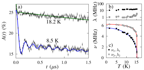
Figure 2: (Color online) a) ZF $\mu^{+}$SR spectra on a polycrystalline sample of Na₂IrO₃ above and below $T_{N}$. Solid lines are (top) guide to the eye and (bottom) a fit described in the text. b,c) Fitted parameters as a function of temperature.

Magnetic order of the Ir spins was detected by zero-field (ZF) muon-spin rotation ($\mu^{+}$SR) on a powder sample of Na₂IrO₃. Example raw spectra are shown in Fig. 2a). At temperatures below $T_{N}=15.3$ K, we observe clear oscillations in the time-dependence of the muon polarization, characteristic of quasi-static local magnetic fields at the muon stopping site. Fits to the time-dependent muon data reveal that two frequencies are present, indicating the presence of two distinct muon stopping sites with different local fields. The full spectra was fitted to the form $A(t)=A_{1}e^{-\lambda_{1}t}\cos(2\pi\nu_{1}t+\phi_{1})+A_{2}e^{-\lambda_{2}t}\cos(2\pi\nu_{2}t+\phi_{2})+A_{3}e^{-\Lambda t}+A_{\mathrm{bg}}$, where the last two terms account for muons polarized parallel to the local magnetic fields, and muons stopping in the sample holder (or cryostat tail), respectively. Using our best-fit parameters we estimate that the muons occupy the two sites with a probability ratio of about 9:1. Both local fields set in at a common temperature, but have a distinctly different temperature dependence [see Fig. 2b)]. The relative weight of the second frequency component suggests that it may come from muon sites implanted near stacking fault planes, as such sites also occur in a similar proportion. Our value for $T_{\rm N}$ is consistent with both susceptibility measurements on the same batch, which indicated a clear anomaly (sharp downturn) near $T_{N}$ as reported previously gegenwart ; Yogesh , and the magnetic Bragg peaks observed in resonant xray scattering hill .

$\begin{array}[]{c}\includegraphics[width=241.84842pt]{fig3_abcd.eps}\\ \includegraphics[width=241.84842pt]{fig3_efghij.eps}\end{array}$

Figure 3: (Color online) Diagram of a) Néel, b) zig-zag and c) stripy order. d) Reciprocal space diagram showing locations of magnetic Bragg peaks for various magnetic phases (inner hexagon shows first Brillouin zone of the honeycomb lattice, $\tilde{a}=a\sin\beta$.) e) Powder inelastic neutron scattering data. The notable well-defined feature is the sharp lower boundary of the scattering at low $Q$ (filled (magenta) symbols in h-j)), which we associate with a sinusoidal spin wave dispersion; this becomes damped out in the paramagnetic phase in f). Slanted thick dashed arrow shows the scan direction in g). Gray shading marks the inaccessible region close to the elastic line dominated by incoherent elastic scattering. g) Energy scan (solid points 4.6 K, open symbols 55 K) through the maximum spin-wave energy seen in e) fitted to a Gaussian peak (solid line), dashed line is estimated background. h-j) Calculated spherically-averaged spin-wave intensity supplementary for the $J_{1,2,3}$ model with h) zig-zag or i) stripy order, and j) the KH model with stripy order for parameters given in the text. Solid red line in j) highlights the low-energy boundary, which coincides with the dispersion from $\Gamma$ to the first softening point.

The magnetic excitations were probed by powder inelastic neutron scattering using the direct-geometry time-of-flight spectrometer MARI at ISIS with an optimised setup to minimise absorption supplementary . Fig. 3e) shows the raw neutron scattering intensity as a function of wavevector ($Q=|\bm{Q}|$) and energy transfer deep in the ordered phase. An inelastic signal with a sinusoidal-like dispersive boundary below a maximum near 5 meV is clearly observed at low $Q$. A gap, if present is smaller than 2 meV. The magnetic character of the scattering is confirmed by the broad, damped-out signal observed in the paramagnetic phase at 55 K [see Fig. 3f) and g) (contrast filled and open symbols)]. Interestingly, the dispersion boundary extrapolates at the lowest energies to a wavevector $Q$ much smaller than that expected for conventional Néel order, $Q_{(020)}=1.34$ Å^-1, so this magnetic order can be ruled out; in fact $Q$ is close to the expected location of the first magnetic Bragg peak for both zig-zag or stripy order, $Q_{(010)}=0.67$ Å^-1. Figs. 3h) and i) show the calculated scattering from spin waves of a 2D Heisenberg model with up to 3rd neighbour exchanges, $J_{1,2,3}$, with zig-zag ($J_{1}=4.17$ meV, $J_{2}/J_{1}=0.78$, $J_{3}/J_{1}=0.9$) and stripy order ($J_{1}=10.89$ meV, $J_{2}/J_{1}=0.26$, $J_{3}/J_{1}=-0.2$), respectively (we neglect the interlayer couplings believed to be small). The constraints to reproduce the dispersion maximum and the measured Curie-Weiss (CW) temperature ($\Theta=-S(S+1)(J_{1}+2J_{2}+J_{3})/k_{\mathrm{B}}\sim-125$ K Yogesh ) are not sufficient to determine all 3 exchanges, so the values chosen are representative of the level of agreement that can be obtained supplementary . The calculation for the zig-zag phase [Fig. 3h)] can reproduce well the observed dispersion at low-$Q$ (filled symbols), whereas the stripy phase [Fig. 3i)] cannot account for the strong low-$Q$ dispersive signal and predicts stronger scattering at larger-$Q$’s not seen. Calculations for the KH Hamiltonian (1) are shown in Fig. 3j) for $\alpha=0.4$ (lower limit for the stripy phase) and $J_{1}=25.85$ meV to reproduce the CW temperature trebst_chi $\Theta=-S(S+1)(J_{1}-J_{\mathrm{K}}/3)/k_{\mathrm{B}}$. The lower boundary of the scattering at low $Q$ (solid line) is predicted to have a quadratic shape near the first softening point, a robust feature for any $\alpha$ throughout the stripy phase. This is in contrast to the data where the dispersion boundary (marked by filled symbols) has a distinctly different, sinusoidal-like shape with a curvature the opposite way. In addition, a different distribution of scattering weight to higher energies is predicted, but not seen in the data. We conclude that the KH model in the stripy phase has a qualitatively different spin-wave spectrum compared to the data. A minimal model that can reproduce the observed low-$Q$ dispersion and which predicts distribution of magnetic scattering in broad overall agreement with the data up to some intensity modulations is shown in Fig. 3h) and requires substantial couplings up to 3rd neighbors, which stabilize zig-zag magnetic order. Recent theory Kimchi proposed that in addition to couplings up to 3rd neighbors, a Kitaev term may also exist. We have compared the data with such a model as well supplementary and estimate that a Kitaev term, if present, is smaller than an upper bound corresponding to $\alpha\lesssim 0.40(5)$.

We note that sizeable $J_{3}$’s are not uncommon in triangular plane metal oxides. The reason is that even though $J_{1}$ involves two hoppings and $J_{3}$ four, the two additional hoppings are strong $pd\sigma$ ones, and the hopping proceeds through intermediate unoccupied $e_{g}$ states NiGa . In case of Na₂IrO₃ the hopping proceeds through somewhat higher Na $s$ orbitals, but these are very diffuse, and the corresponding $t_{sp\sigma}$ parameter is sizeable. Near cancellation of the AFM and FM superexchange interaction for the nearest-neighbor path further reduces $J_{1}$ compared to $J_{3}$.

To summarize, by combining single-crystal diffraction and LDA calculations we proposed a revised crystal structure for the spin-orbit coupled honeycomb antiferromagnet Na₂IrO₃ that highlights important departures from the ideal case where the Kitaev exchange dominates. We observed dispersive spin-wave excitations in inelastic neutron scattering and showed that substantial further-neighbor exchange couplings are required to explain the observed dispersion and we proposed a model for the magnetic ground state that could support such a dispersion relation.

We thank G. Jackeli for providing notes on spin-wave dispersions for the KH model in the rotated frame, A. Amato for technical support, N. Shannon, J.T. Chalker and L. Balents for discussions, and EPSRC for funding. Work at Rutgers was supported by DOE (DE-FG02-07ER46382).

Supplemental Material for Spin waves and revised crystal structure of honeycomb iridate Na₂IrO₃

Here we provide additional information on 1) structural optimization calculations to confirm the unit cell stability and estimate the energy of stacking faults, 2-3) the xray diffraction measurements and analysis of the diffuse scattering, 4) $\mu$SR and 5) neutron scattering experiments, and 6-9) derive the spin-wave dispersion relations and dynamical structure factor in neutron scattering for the Heisenberg $J_{1,2,3}$, Kitaev-Heisenberg and Kitaev-Heisenberg-$J_{2}$-$J_{3}$ models for various magnetic orders.

Figure S1: (Color online) Radial distribution functions (RDFs) showing the difference in the local atomic environments for the previously reported $C2/c$ structure S (4) and the $C2/m$ structure proposed in this study. In the $C2/m$ case, the RDFs are plotted for the unit cell extracted from the experiment (red solid line), the unit cell with atomic positions relaxed in the DFT (blue dashed line), and the unit cell fully relaxed in the DFT (green dotted line). Note that a small Gaussian smearing ($\sigma=0.008$Å) was used in the calculation of the RDFs.

S1. Structural optimization calculations using VASP

We used the Perdew-Burke-Ernzerhof (PBE) exchange-correlation functional S (1) within the generalized gradient approximation (GGA) and the projector augmented waves method S (2). The $2p$ semi-core electrons in Na were treated as valence. Numerical convergence was achieved with a 500 eV energy cutoff and dense Monkhorst-Pack $k$-meshes S (3) of 7$\times$7$\times$3 for the previously reported S (4) $C2/c$ primitive unit cell and 6$\times$4$\times$6 for the proposed $C2/m$ conventional unit cell in Table I. We performed three types of calculations for the two structures: a static run with the experimental parameters, optimization of the atomic positions only, and full optimization of the atomic positions and lattice parameters. The residual forces and stresses were typically below 0.002 eV/Å and 0.5 kbar, respectively. We found the magnetic and the spin-orbit interactions to have a rather small effect on the Na₂IrO₃ structure and the comparisons below are made for the non-magnetic case without the spin-orbit coupling.

To illustrate the differences in the local environments in Fig. S1 we plotted normalized radial distribution functions (RDFs) for all types of interatomic distances in the experimental and optimized structures. $C2/c$ exhibits a considerable dispersion of the Ir-Ir and Ir-O nearest neighbor distances critical for the magnetic ordering in the compound. The O-Na and Na-Na separations are unphysically small and we observed large forces, over 6 eV/Å on Na and over 3 eV/Å on O, at the beginning of the optimization run. The RDFs in $C2/m$ with the experimental parameters demonstrate much more symmetric local environments and a negligible variation of Ir-Ir lengths within the honeycomb lattice (below 0.3%). The calculated forces on atoms did not exceed 0.5 eV/Å indicating a good agreement between the experiment and theory. Optimization of the atomic positions with fixed $C2/m$ experimental unit cell had little effect on the Ir-Ir distances because they are defined primarily by the in-plane lattice constants $a$ and $b$. When fully optimized, $C2/c$ and $C2/m$ converged to the same structure with the $C2/m$ space group and virtually indistinguishable RDFs. The enthalpy gains were 0.434 and 0.018 eV/atom, respectively (for comparison, the optimization of atomic positions in $C2/m$ led to a 0.007 eV/atom gain). Note that the full optimization of $C2/m$ leads to $\sim$ 2% elongation of the Ir-Ir distances which is a typical bond overestimation observed for the GGA. For this reason we believe that use of the experimental lattice constants is more appropriate for the modelling of the magnetic interactions.

To estimate the stacking fault energy we simulated 1$\times$1$\times$$n$ ($n=2,\dots,6$) supercells of the $C2/m$ primitive 12-atom unit cell with one Ir-Na layer and the two adjacent O layers shifted by $b/3$ along [010]. The resulting lower-symmetry structures ($C2$ space group) had two stacking faults per unit cell and the same $a\times b/2=25.49$Ų $x-y$ base. We optimized only the atomic positions keeping the experimental unit cell parameters fixed. The $n=2$ structure gained additional symmetry operations ($C2/c$ space group) upon relaxation. The comparison of the faulted structures against the respective $C2/m$ supercells with the same unit cell dimensions and the same $k$-point meshes allowed us to reduce computational errors. However, the energy differences, $E_{n}-E_{C2/m}$, in our non-magnetic calculations without the spin-orbit coupling (SOC) proved to be exceptionally small in magnitude: 0.7, -1.7, -2.0, -2.6, -1.8 meV/($n\times 12$ atoms) for $n=2,\dots,6$, respectively. For the smallest $n=2$ structure we were able to calculate the energy difference with the FM ordering and the SOC as well and found $E_{n=2}-E_{C2/m}$ to remain small at 2.9 meV/(24 atoms). Based on these tests, we expect the stacking fault energy in $C2/m$ to be below $\sim$ 0.1 meV/Ų, one to two orders of magnitude smaller than typical stacking fault energies for elemental metals. For comparison, an ABCBA stacking fault generated by reflecting $C2/m$ structure (which has the ABCABC sequence along $c$) about a Na layer was calculated to have a much higher, measurable energy value of about 8 meV/Ų.

S2. Xray diffraction and structural analysis

Figure S2: (Color online) Xray diffraction intensity in the ($-3,k^{\prime},l^{\prime}$) plane: a) data, b) calculation for the “idealized” C$2/c$ structure with atoms at special positions, equivalent to the C$2/m$ model in Table I, c) calculation for the distorted C$2/c$ model in S (4) (assuming no Ir/Na site mixing in the honeycomb Ir_2/3Na_1/3 layers). Notice the series of sharp peaks predicted in c) at (-3,1,even) positions, which however are not present in the data in a). d) Scan along the (-3,1,$l^{\prime}$) line (arrowed direction in a-c)) comparing data (solid circles) and calculation for the two models (triangles-C$2/c$ and squares-C$2/m$). The calculated diffraction intensities have been multiplied by an overall scale factor and have been convolved with a finite width Gaussian in momentum space to mimic the effects of the instrumental resolution.

X-ray diffraction was performed using a Mo-source Oxford Diffraction Supernova diffractometer on a single crystal of Na₂IrO₃ of approximate size 220$\times$150$\times$10$\mu$m³ grown via flux S (4). 96$\%$ out of over 1000 detected peaks were indexed by a single monoclinic domain. Structural refinement was performed using both a unit cell with space group C$2/m$, with parameters listed in Table I, as well as a unit cell with twice the volume and space group C$2/c$, using the SIR-92 and SHELX packages S (5). The two unit cell parameters are related by ${\bm{a}^{\prime}}=-\bm{a}$, ${\bm{b}^{\prime}}=-\bm{b}$, ${\bm{c}^{\prime}}=\bm{a}+2\bm{c}$, $c^{\prime}=\sqrt{a^{2}+4c^{2}+4ac\cos\beta}$, $\sin\beta^{\prime}=\frac{2c}{c^{\prime}}\sin\beta$, and in terms of the reciprocal lattice components $h^{\prime}=-h$, $k^{\prime}=-k$, $l^{\prime}=h+2l$, where primed values refer to the C$2/c$ model. Starting from the larger unit cell (C$2/c$) and slightly displacing the atoms to some “ideal” positions one recovers the higher-symmetry structure described by the smaller, C$2/m$, cell. The distinction between those two models is entirely due to such small atomic displacements, the presence of which is manifested in finite intensity diffraction peaks at ($h^{\prime},k^{\prime},l^{\prime}$) positions with $h^{\prime}$ odd, $k^{\prime}$ odd and $l^{\prime}$ even, which disappear when atoms are displaced to the “ideal” positions, when the structure recovers the C$2/m$ symmetry. This is illustrated by the calculated diffraction pattern in the ($-3,k^{\prime},l^{\prime}$) plane where the “extra” peaks expected in the larger cell model C$2/c$ shown in Fig. S2c) are not seen in the data plotted in Fig. S2a), which is however fully consistent with the pattern expected for the higher-symmetry C$2/m$ model shown in Fig. S2b). This is also apparent in Fig. S2d) showing a scan along the ($-3,1,l^{\prime}$) line with extra peaks (triangles) predicted for $l^{\prime}=0,2$, not seen in the data (filled symbols). For completeness we note that we applied a shift of the fractional atomic coordinates in the C$2/c$ unit cell (in the notation adopted in S (4)) by (-1/4,-3/4,0) before converting them into fractional atomic coordinates of the C$2/m$ cell (in the notation used in Table I), due to the different positions of the origin in the two space groups.

S3. Microscopic model of stacking faults

The calculated diffraction pattern in Fig. 1e) was obtained numerically by direct structure-factor calculations using the DISCUS package S (6). We considered a “crystal” of $200a\times 200b\times 4000c$ unit cells of Na₂IrO₃ (C$2/m$). To include the effect of stacking faults we assumed that each Ir layer has a choice with probability $1-p$ to keep in-stacking-sequence with the layer below and $p/2$ to be shifted to either of the other two sublattice positions (translated in-plane by $(0,1/3,0)$ or $(1/2,1/6,0)$), with $p=0$ for perfect stacking and $p=1/3$ for a completely uncorrelated layer stacking sequence, a model first introduced to describe the stacking faults in the related material Li₂MnO₃ S (7).

S4. Muon spin relaxation experiments

Zero field (ZF) $\mu^{+}$SR measurements were made at the Swiss Muon Source (S$\mu^{+}$S), Paul Scherrer Institut, CH using the GPS spectrometer. For the measurement a 250 mg powder sample of Na₂IrO₃, which was used for inelastic neutron scattering measurement, was packed inside a silver foil packet (foil thickness 25$~{}\mu$m) and mounted on a silver sample holder.

Fits of the data to an equation in main text reveal the evolution of $\nu_{i}$ and $\lambda_{i}$ with temperature, as shown in Figs. 2(b-c). Unusually, the frequencies do not vary in fixed proportion, although they do tend to zero at the same temperature. The low-amplitude, higher frequency component $\nu_{2}$ drops off far more dramatically than the large amplitude, lower frequency $\nu_{1}$. In order to quantify this behavior, the frequencies were fitted to the phenomenological function $\nu_{i}(T)=\nu_{i}(0)\left[1-\left(T/T_{\mathrm{N}}\right)^{\alpha_{i}}\right]^{\beta_{i}}$. A common value of $T_{\mathrm{N}}=15.3(1)$ K was identified from fitting to this function. We find that $\alpha\approx 2$ for both cases. The parameter $\beta$ can be interpreted as an order parameter exponent. The other fit parameters are $\nu_{1}(0)=5.54(1)$ MHz, $\beta_{1}=0.36(1)$, $\nu_{2}(0)=6.20(3)$ MHz and $\beta_{2}=0.11(1)$. We note that $\lambda_{1}$ is an order of magnitude larger than $\lambda_{2}$, implying either that the distribution of fields is broader in the majority site or, assuming the fast fluctuation limit, that the fluctuation rate is smaller. The lower frequency oscillation, accounting for $\approx 90$% of the muon sites in the material, has a $\beta$ value suggestive of the behavior of a three-dimensional (3D) system (for 3D Heisenberg $\beta=0.367$ and 3D Ising $\beta=0.326$), while the minority muon site has an exponent value more similar to that expected for a 2D Ising system (for which $\beta=0.125$). These seem to suggest that the magnetic fluctuations have a rather different character at the two muon sites.

S5. Inelastic neutron scattering experiments

Inelastic neutron scattering measurements were made using the direct-geometry time-of-flight spectrometer MARI at ISIS using an incident neutron energy of 18 meV, which covered the full bandwidth of magnetic excitations with a zone boundary energy near 5 meV. The instrumental energy resolution was 0.67(1) meV (FWHM) on the elastic line. The sample was $\sim 10$ g of Na₂IrO₃ powder spread out in a very thin layer ($\lesssim 1$ mm to minimise neutron absorption) inside of an annular can of outer diameter of 40 mm and height 50 mm. Counting times for the data in Figs. 3e-f) were 28 and 7 hours, respectively, at an average proton current of $150\mu$Amps.

S6. Spin-wave dispersions for the Heisenberg $J_{1,2,3}$ model in the zig-zag and stripy phases

Here we outline the derivation of the linear spin wave dispersion relations and dynamical structure factors relevant for neutron scattering for various spin Hamiltonians on the honeycomb lattice. For the Heisenberg model with up to 3rd neighbour exchanges we extend previous results on the dispersion relations S (8) to include also the dynamical structure factors. For the Kitaev-Heisenberg model the spin-wave spectrum (including $1/$S quantum corrections) has been studied before in a special “rotated” reference frame S (9), here we explicitly derive here the dispersion relations and dynamical structure factors in the experimentally-relevant, un-rotated reference frame. For the Kitaev-Heisenberg-$J_{2}$-$J_{3}$ models both the dispersion relations and dynamical structure factors have not been studied before.

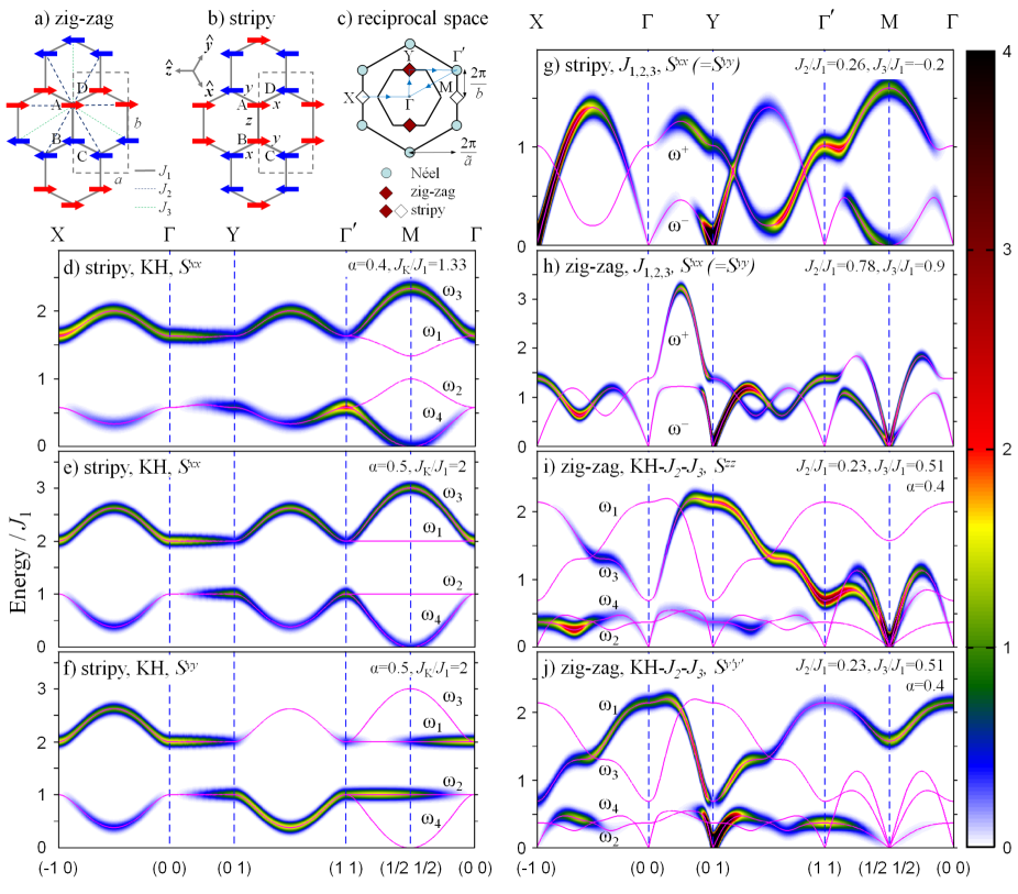
Figure S3: (Color online) a) Zig-zag and b) stripy order. Dashed rectangular box of size $a\times b$ shows the magnetic unit cell containing four sublattices A-D. In a) solid, dashed and dot-dashed lines show paths for $J_{1}$, $J_{2}$ and $J_{3}$. b) Bond labels $x,y,z$ refer to the components of the spins at the two bond ends coupled by the Kitaev term. Inset show projection of the (cubic) $\hat{\bm{x}}$, $\hat{\bm{y}}$ and $\hat{\bm{z}}$ axes onto the honeycomb plane. c) 2D reciprocal space showing magnetic Bragg peak positions for various magnetic orders, $\tilde{a}=a\sin\beta$. d-j) Spin-wave dispersions along symmetry directions in reciprocal space (arrowed path in c)) for the KH, $J_{1,2,3}$ and KH-$J_{2}$-$J_{3}$ Hamiltonians for exchange values and magnetic orders listed in the legends. Wavevectors $\bm{Q}$ are expressed in reciprocal lattice units of the rectangular magnetic unit cell. Colour is the dynamical structure factor (convolved with a Gaussian in energy for visualization, full width at half maximum $=0.15J_{1}$), isotropic for the Heisenberg model in g-h) ($S^{xx}(\bm{Q},\omega)=S^{yy}(\bm{Q},\omega)$) and different for the two polarizations $x,y$ for the KH model in d-f). i-j) Dynamical structure factor for the KH-$J_{2}$-$J_{3}$ model with the zig-zag structure in a), where the ordered moments are along a general direction $x^{\prime}$ in the $xy$ plane and $y^{\prime}$ is a direction in this plane normal to $x^{\prime}$.

We start with the isotropic Heisenberg model on the honeycomb lattice with exchanges with up to 3rd nearest-neighbor, so called $J_{1,2,3}$ model with Hamiltonian

$${\cal H}=\sum_{\rm{1NN}}J_{1}{\bm{S}}_{i}\cdot\bm{S}_{j}+\sum_{\rm{2NN}}J_{2}{\bm{S}}_{i}\cdot\bm{S}_{k}+\sum_{\rm{3NN}}J_{3}{\bm{S}}_{i}\cdot\bm{S}_{l}$$ (S1)

where 1-, 2-, and 3NN indicate summing over all 1st, 2nd and 3rd nearest-neighbor pairs with couplings $J_{1}$, $J_{2}$ and $J_{3}$ [paths indicated in Fig. S3a)], where positive values correspond to antiferromagnetic exchanges. Depending on the relative ratio of the couplings there are six distinct types of mean-field ground states S (8, 10), which include the two candidate magnetic orders for Na₂IrO₃, the zig-zag and stripy AFM orders shown in Figs. S3a-b) (labelled II and IV, respectively, in S (8, 10)). Both of those magnetic structures have four magnetic sublattices (labelled A-D) and can be described by a rectangular magnetic unit cell (dashed box in Figs. S3a-b)), which coincides with the in-plane chemical unit cell $a\times b$ of Na₂IrO₃. Within a single layer the Ir honeycomb lattice in very close to ideal ($b/a\simeq\sqrt{3}$) in spite of the 3D monoclinic crystal structure, so we treat here the ideal 2D honeycomb lattice with 3-fold symmetry. In this case the magnetic order can have three spacial domains, one such domain is shown for both structures in Figs. S3a-b), the other two magnetic domains are obtained by $\pm 60^{\circ}$ rotation around the direction normal to the plane.

Using a standard Holstein-Primakoff transformation in the large-$S$ limit the Hamiltonian becomes (to leading order) a quadratic form of magnon operators

$$\mathcal{H}=\sum_{\bm{q}}\mathsf{X}^{\dagger}\mathsf{H}\mathsf{X}+N(1+1/S)E_{MF}$$ (S2)

where higher than quadratic terms are neglected. Here $E_{MF}$ is the mean-field ground state energy (per spin) and $N$ is the total number of spin sites. The sum extends over all wavevectors ${\bm{q}}$ in the first magnetic Brillouin zone.

For the zig-zag order in Fig. S3a) we define the operator basis as $\mathsf{X^{\dagger}}=\left[a^{\dagger}_{\bm{q}}~{},~{}d^{\dagger}_{\bm{q}}~{},~{}c_{-\bm{q}}~{},~{}b_{-\bm{q}}\right]$ where $a-d$ label operators on sublattice A-D, i.e. $a^{\dagger}_{\bm{q}}$ ($a_{\bm{q}}$) creates (annihilates) a plane-wave magnon mode on sublattice A and so on. The Hamiltonian matrix in eq. (S2) is

$$\mathsf{H}=\left[\begin{array}[]{llll}A&B&C&D^{*}\\ B^{*}&A&D&C\\ C&D^{*}&A&B\\ D&C&B^{*}&A\\ \end{array}\right]$$ (S3)

where

$$\begin{array}[]{l l}A&=S\ \{-J_{1}+2J_{2}+3J_{3}+2J_{2}\cos(2\pi h)\}\\ B&=2SJ_{1}\eta\cos(\pi h)\\ C&=2SJ_{2}\{\cos\left[\pi(h+k)\right]+\cos\left[\pi(h-k)\right]\}\\ D&=S\ \{J_{1}{\eta}^{2}+J_{3}\left[{{\eta}}^{-4}+2{{\eta}}^{2}\cos(2\pi h)\right]\}\\ \eta&=e^{k\pi i/3}.\end{array}$$

Here $(h,k)$ are components of the wavevector ${\bm{q}}$ in units of the reciprocal lattice of the $a\times b$ rectangular unit cell shown in Fig. S3a). By periodicity the above expressions are valid for any momentum, not necessarily restricted to the 1st magnetic Brillouin zone. Diagonalisation of the Hamiltonian by standard techniques S (11, 12) to obtain the normal magnon modes gives two doubly-degenerate dispersions

$$\begin{array}[]{ll}(\omega^{\pm}_{\bm{q}})^{2}&=A^{2}+BB^{*}-C^{2}-DD^{*}\\ &\pm\sqrt{4|AB-CD^{*}|^{2}-|B^{*}D^{*}-BD|^{2}}.\end{array}$$ (S4)

We have explicitly verified for the same model (S1) that eq. (S4) agrees with earlier results of S (8) [eq. (5.21)]. The spin-wave intensity in neutron scattering is proportional to the dynamical structure factor (expressed as $S^{xx}({\bm{Q}},\omega)$ for spin fluctuations along the $x$-direction and similarly for $y$-direction) and an analytical expression for this in the case of a Hamiltonian of the form in eq. (S3) are given explicitly S (12) [eq. (A3)] and for brevity are not included here.

The spin-wave dispersions in (S4) (and their intensity dependence) for the zig-zag phase are plotted for representative exchange values in Fig. S3h). As expected, the acoustic magnon, $\omega^{-}$, is gapless with a linear dispersion at the magnetic Bragg peak at the Y point, is also linear and gapless at the X point, but has zero intensity because the structure factor for magnetic Bragg peaks also cancels at this position. Furthermore, the dispersions soften and appear gapless at the M point and others part of the quartet ($\pm 1/2,\pm 1/2$), which are Bragg peaks for the other two magnetic domains rotated by $\pm 60^{\circ}$. This softening is a general feature of linear spin-wave dispersions for a multi-domain magnetic ground state S (12), however the fact that the gap closes at those points is not protected by any symmetry, but is an artefact of the linear spin-wave approximation; by analogy with related spin-wave models for other multi-domain structures S (13) we expect the dispersions to become gapped at the softening points when quantum fluctuations to 1st order in 1/$S$ are included.

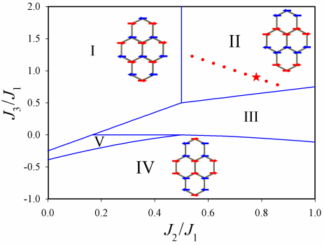
Figure S4: (Color online) Classical phase diagram of the Heisenberg $J_{1,2,3}$ model on the honeycomb lattice, eq. (S1), showing the regions of stability for zig-zag (II) and stripy order (IV). Phase I is collinear $2$-sublattice Néel order, III and V are incommensurate spiral phases, and solid lines are phase boundaries S (10). The dotted line inside region II indicates possible solutions for a minimal model to describe the spin dynamics in Na₂IrO₃ obtained by imposing the constraints described in the text (the red star is a representative solution for which the full spectrum is shown in Fig. S3h)).

A spherical average of the spin-wave spectrum (including various prefactors listed in eq. (S9) below) is shown in Fig. 3h). The dominant contribution to the low-$Q$ dispersive edge of the strong signal near the first softening point ($Q$=0.67 Å^-1) is due to acoustic magnons on the $\omega^{-}_{\bm{k}}$ branch emerging out of the Y point and dispersing in the Y$\rightarrow\Gamma$ direction [see Fig. S3h)] and also magnons on the $\omega^{+}_{\bm{k}}$ branch emerging out of the M-point and dispersing in the M$\rightarrow\Gamma$ direction. To reproduce the observed low-$Q$ dispersion in the powder data we have imposed the constraint that the zone-boundary energy of the lowest branch on the $\Gamma$-Y line reproduces the observed maximum of the low-$Q$ dispersion, i.e. $\omega^{-}\left(0,\frac{1}{2}\right)=5$ meV. This constraint together with the condition that the exchanges reproduce the observed Curie-Weiss constant $\theta=-S(S+1)(J_{1}+2J_{2}+J_{3})/k_{\rm B}=-125$ K cannot determine all three exchange values $J_{1}$, $J_{2}$ and $J_{3}$, but allow for a one-dimensional family of solutions located on a curve in the parameter space $(J_{2}/J_{1},J_{3}/J_{1})$ (the dotted line in region II in Fig. S4). All sets of exchange values part of this family are broadly consistent with the data. The level of agreement that can be obtained is illustrated in Fig. 3h) for one representative solution (red star in Fig. S4), chosen as it comes closest to reproducing also the intensity distribution at the lowest $Q$.

We now turn to the alternative magnetic structure, the stripy order shown in Fig. S3b). If the spin-wave operator basis is defined as $\mathsf{X^{\dagger}}=\left[a^{\dagger}_{\bm{q}}~{},~{}b^{\dagger}_{\bm{q}}~{},~{}c_{-\bm{q}}~{},~{}d_{-\bm{q}}\right]$, then the Hamiltonian reduces to the same form as in eqs. (S2,S3), with magnon dispersions given by eq. (S4), but where the expressions for the $A-D$ parameters are

$$\begin{array}[]{l l}A&=S\ \{J_{1}+2J_{2}-3J_{3}+2J_{2}\cos(2\pi h)\}\\ B&=S\ \{J_{1}\eta^{-2}+J_{3}\left[\eta^{4}+2\eta^{-2}\cos(2\pi h)\right]\}\\ C&=2SJ_{2}\{\cos\left[\pi(h+k)\right]+\cos\left[\pi(h-k)\right]\}\\ D&=2SJ_{1}{\eta}^{-1}\cos(\pi h)\\ \eta&=e^{k\pi i/3}.\end{array}$$

The resulting spin-wave dispersions and intensities for representative exchange values are plotted in Fig. S3g). In contrast to the zig-zag phase, for the stripy phase the acoustic magnon, $\omega^{-}$, is gapless, with a linear dispersion and finite intensity at both the X and Y points, as both are magnetic Bragg peaks with non-zero structure factor (X four times stronger intensity than Y). Again, due to the three domain structure there is softening of the dispersion with an artificial gapless point at M, which is expected to become gapped when quantum fluctuations beyond the linear spin-wave approximation are included, as discussed earlier. A spherical averaging of the spin-wave spectrum in Fig. S3g) is shown in Fig. 3i), here the strongest signal at low energies is due to scattering from acoustic magnons near the X-point ($Q=1.16$ Å^-1) with weaker scattering from magnons near Y ($Q=0.67$ Å^-1) and intensity decreasing rapidly for magnons with smaller momentum.

S7. Spin-wave dispersions for the Kitaev-Heisenberg model in the stripy phase

For the nearest-neighbor Kitaev-Heisenberg (KH) model in eg. (1) the stripy phase in Fig. S3b) is the stable ground state for $0.4\lesssim\alpha\lesssim 0.8$, where $\alpha=J_{\mathrm{K}}/\left(J_{\mathrm{K}}+2J_{1}\right)$ S (9). This ground state is exact at $\alpha=0.5$, when upon rotation of the coordinate system at certain sites the Hamiltonian (1) converts to that of a Heisenberg ferromagnet in a rotated basis S (9).

For each of the three bonds coming out of a honeycomb lattice site the Kitaev term $J_{\rm K}$ couples different spin components $x,y,z$ expressed in terms of an orthogonal (cubic) reference frame. This is oriented with the cubic [111] axis normal to the honeycomb plane and the projections of the $\hat{\bm{x}}$, $\hat{\bm{y}}$ and $\hat{\bm{z}}$ axes in the plane making $120^{\circ}$ as shown in Fig. S3b) inset. Each bond is labelled with the type of the spin component for the moments at the two bond ends coupled by the Kitaev term, i.e. the $z$-bond AB stands for exchange $-J_{\rm K}S^{z}_{A}S^{z}_{B}$ and $x$-bond AD stands for $-J_{\rm K}S^{x}_{A}S^{x}_{D}$ and so on.

Due to the anisotropic nature of the Kitaev exchange more coupling terms between magnon operators on the 4 different magnetic A - D sublattices are generated as compared to the Heisenberg $J_{1,2,3}$ model. Thus, one needs to use the full 8-term operator basis $\mathsf{X}^{\dagger}=\left[a_{\bm{q}}^{\dagger}~{},~{}b_{\bm{q}}^{\dagger}~{},~{}c_{\bm{q}}^{\dagger}~{},~{}d_{\bm{q}}^{\dagger}\\ ~{},~{}a_{-\bm{q}}~{},~{}b_{-\bm{q}}~{},~{}c_{-\bm{q}}~{},~{}d_{-\bm{q}}\right]$, for which the Hamiltonian expressed in magnon operators to leading order still has the quadratic form (S2) with the matrix $\mathsf{H}$ given by

$$\mathsf{H}=\frac{1}{2}\left[\begin{array}[]{llllllll}A&B&0&C&0&0&0&D\\ B^{*}&A&C^{*}&0&0&0&D^{*}&0\\ 0&C&A&B&0&D&0&0\\ C^{*}&0&B^{*}&A&D^{*}&0&0&0\\ 0&0&0&D&A&B&0&C\\ 0&0&D^{*}&0&B^{*}&A&C^{*}&0\\ 0&D&0&0&0&C&A&B\\ D^{*}&0&0&0&C^{*}&0&B^{*}&A\\ \end{array}\right]$$ (S5)

where

$$\begin{array}[]{l l}A&=S\left(J_{1}+J_{\rm{K}}\right)\\ B&=SJ_{1}\eta^{-2}\\ C&=-SJ_{\rm{K}}i\sin\left(\pi h\right)\eta\\ D&=S\left(2J_{1}-J_{\rm{K}}\right)\cos\left(\pi h\right)\eta\\ \eta&=e^{k\pi i/3}.\\ \end{array}$$

Diagonalization to get the normal magnon modes S (11) gives four dispersion relations

$$\begin{array}[]{ll}\omega_{1,2}^{2}({\bm{q}})=A^{2}-DD^{*}+|B-C|^{2}\\ \pm\sqrt{4A^{2}|B-C|^{2}-|D^{*}(B-C)-D(B^{*}-C^{*})|^{2}}\\ \omega_{3,4}^{2}({\bm{q}})=A^{2}-DD^{*}+|C+B|^{2}\\ \pm\sqrt{4A^{2}|B+C|^{2}-|D^{*}(B+C)-D(B^{*}+C^{*})|^{2}}.\\ \end{array}$$ (S6)

The dispersion curves are plotted for $\alpha=0.4$ in Fig. S3d) and $\alpha=0.5$ in Figs. S3(e-f), where the colour represents the dynamical structure factor, plotted separately for the spin fluctuations along $x$ and $y$-axes, the presence of Kitaev bond directional exchanges make those the dynamical structure factor non-equivalent. The structure factors were obtained from the eigenvectors of the Hamiltonian matrix $\mathsf{H}$ in eq. (S5), using a numerical implementation of a general algorithm to diagonalize a quadratic form of boson operators proposed in S (14). Changing the relative strength of the Kitaev term, for example $\alpha=0.4$ compared to 0.5, does not change the spectrum qualitatively only introduces a weak dispersion in the gapped $\omega_{1,2}$ modes, compare Figs. S3d-e).

The dispersions show many distinct features compared to the case when the same stripy ground state was stabilized instead by isotropic Heisenberg exchanges shown in Fig. S3g). Notably there is no longer a gapless mode at the $\Gamma$ point and at the Bragg peak positions (X and Y). The lowest mode softens at the M point as in previous cases due to the 3-domain structure of the stripy ground state. The dispersion is gapless at this point in the linear spin-wave approximation and a gap is predicted to open up when quantum fluctuations to 1st order in $1/S$ are included for any general $\alpha$, except for the exactly solvable point $\alpha=0.5$ where due to an exact cancellation the spectrum is gapless S (9).

A spherical average of the spin-wave spectrum in Fig. S3d) (including both the $S^{xx}$ and $S^{yy}$ dynamical structure factors) is shown in Fig. 3j), the lower boundary of the scattering at low-$Q$ (emphasized by the red solid line) is due to scattering off magnons on the $\omega_{4}$ $\Gamma$-M dispersion branch near the M point.

S8. Spin-wave dispersions for the Kitaev-Heisenberg-$J_{2}$-$J_{3}$ model in the zig-zag phase

Here we explore the effects of adding a small Kitaev interaction $J_{\rm K}$ to the $J_{1,2,3}$ Hamiltonian when the ground state order is the zig-zag phase (this has recently been shown to be stable for a range of $J_{\rm K}$ values S (15)). We obtain the spin-wave Hamiltonian matrix in this case by combing eqs. (S3) and (S5) as

$$\mathsf{H}=\frac{1}{2}\left[\begin{array}[]{llllllll}A&B&0&C&0&D&E&F\\ B^{*}&A&C^{*}&0&D^{*}&0&F^{*}&E\\ 0&C&A&B&E&F&0&D\\ C^{*}&0&B^{*}&A&F^{*}&E&D*&0\\ 0&D&E&F&A&B&0&C\\ D^{*}&0&F^{*}&E&B^{*}&A&C^{*}&0\\ E&F&0&D&0&C&A&B\\ F^{*}&E&D^{*}&0&C^{*}&0&B^{*}&A\\ \end{array}\right]$$ (S7)

where

$$\begin{array}[]{l l}A&=S\ \{-J_{1}+2J_{2}+3J_{3}+2J_{2}\cos(2\pi h)+J_{\rm{K}}\}\\ B&=(-1/2)SJ_{\rm{K}}{\eta}^{-2}\\ C&=S\ \{2J_{1}\cos(\pi h)-(1/2)J_{\rm{K}}{\zeta}\}{\eta}\\ D&=S\ \{J_{1}{\eta}^{-2}+J_{3}\left[{{\eta}}^{4}+2{{\eta}}^{-2}\cos(2\pi h)\right]-J_{\rm{K}}{\eta}^{-2}/2\}\\ E&=2SJ_{2}\{\cos\left[\pi(h+k)\right]+\cos\left[\pi(h-k)\right]\}\\ F&=(1/2)SJ_{\rm{K}}{\zeta}{\eta}\\ \zeta&=e^{h\pi i}\\ \eta&=e^{k\pi i/3}.\end{array}$$

Diagonalization leads to four dispersion branches

$$\begin{array}[]{ll}\omega_{1,2}^{2}({\bm{q}})&=A^{2}-E^{2}+|B-C|^{2}-|D-F|^{2}\\ &\pm\sqrt{4|A(B-C)+E(D-F)|^{2}-\delta_{-}^{2}}\\ \omega_{3,4}^{2}({\bm{q}})&=A^{2}-E^{2}+|B+C|^{2}-|D+F|^{2}\\ &\pm\sqrt{4|A(B+C)-E(D+F)|^{2}-\delta_{+}^{2}}\\ \end{array}$$ (S8)

where $\delta_{\pm}=|(B\pm C)(D^{*}\pm F^{*})-(B^{*}\pm C^{*})(D\pm F)|$. The dispersions are plotted in Figs. S3i-j) for $\alpha$=0.4 ($J_{\rm K}/J_{1}=4/3$), $J_{2}$/$J_{1}$ =0.23 and $J_{3}$/$J_{1}$ =0.51. To discuss the key features of the spectrum it is helpful to visualize the degeneracies associated with the magnetic order. The magnetic structure is the zig-zag pattern shown in Fig. S3a) but where the spin direction can be either along the $\hat{\bm{x}}$ direction to satisfy the Kitaev term on the $x$-type AD bond, or along the $\hat{\bm{y}}$ direction to satisfy the Kitaev exchange on the $y$-type BC bond. At the classical level any in-between direction, i.e. in the $\hat{\bm{x}}\hat{\bm{y}}$ plane, also has the same energy, so one expects a gapless mode associated with rotations in this “easy” plane. Indeed Fig. S3j) shows that the dispersion is gapless at the Y point and with strong intensity for fluctuations in this easy-plane (along the $\hat{\bm{y}^{\prime}}$ normal to the ordered direction labelled $\hat{\bm{x}^{\prime}}$), and gapped for fluctuations along $\hat{\bm{z}}$ out of the easy plane, see Fig. S3i). Furthermore, due to the honeycomb lattice geometry the magnetic structure is degenerate with another two domains rotated by $\pm 60^{\circ}$ around the axis normal to the plane, so the spectrum is gapless at the Bragg peak positions of those other two domains, at points equivalent to M. The Hamiltonian however does not poses any continuous rotational symmetry in the presence of the Kitaev term, so one might expect that small gaps would open at both Y and M points when quantum fluctuations are included so the spectrum would be fully gapped. For completeness we quote the Curie-Weiss temperature for this model $\theta_{\rm CW}=-S(S+1)(J_{1}+2J_{2}+J_{3}-J_{\rm K}/3)/k_{\rm B}$.

S9. Spherically-averaged neutron scattering intensity

The one-magnon neutron scattering intensity including the magnetic form factor and neutron polarization factor is proportional to

$$\left(\frac{g}{2}f(Q)\right)^{2}\left[\left(1-\frac{Q_{x}^{2}}{Q^{2}}\right)S^{xx}(\bm{Q},\omega)+\left(1-\frac{Q_{y}^{2}}{Q^{2}}\right)S^{yy}(\bm{Q},\omega)\right]$$ (S9)

where we used for $f(Q)$ the Ir⁴⁺ spherical magnetic form factor S (16) and assumed the $g$-factor equal to 2. Here $Q_{x}$ ($Q_{y}$) are the components of the wavevector transfer ${\bm{Q}}$ along the $x$-axis ($y$-axis), where $z$ is the ordered spin direction. The precise direction of the ordered moments ($\hat{\bm{z}}$-axis) with respect to the crystallographic axes has only a small effect on the powder-averaged spectrum via small intensity modulations through the polarization factors $\left(1-\frac{Q_{x,y}^{2}}{Q^{2}}\right)$, however for concreteness, we included a specific moment direction for the comparison with data. For the $J_{1,2,3}$ model in Figs. 3(h-i) the moments were assumed to be aligned along the crystallographic ${\bm{a}}$-axis (as suggested by resonant xray data S (17)) and for the KH model [Fig. 3j)] the moment is assumed to be along the cubic $\hat{\bm{z}}$-axis closest to the ${\bm{a}}$-axis (tilted out-of-plane by 35.26^∘ from the ${-\bm{a}}$ axis, see Fig. S3b) inset). Eq. (S9) was numerically averaged over a spherical distribution of orientations for the wavevector transfer $\bm{Q}$ and convolved with the instrumental resolution to obtain the plots in Figs. 3h-j), directly comparable with the raw neutron scattering data in Fig. 3e). For the KH-$J_{2}$-$J_{3}$ model the intensity is also given by eq. (S9) but with the axis labels ($x$,$y$,$z$) replaced by ($y^{\prime}$, $z$, $x^{\prime}$), where the $x^{\prime}$-axis defines the ordered moment direction (located in the original $xy$ plane) and $y^{\prime}$ and $z$ are orthogonal directions to it.

References

- (1)
- (2) [a] Current address: Department of Physics, Durham University, South Road, Durham, DH1 3LE, UK.
- (3)
- (4) [b] Current address: Indian Institute of Science Education and Research Mohali, Sector 81, SAS Nagar, Manauli PO 140306, India.
- (5) D. Pesin, L. Balents, Nature Physics 6, 376 (2010).
- (6) J. Chaloupka, G. Jackeli and G. Khaliullin, Phys. Rev. Lett. 105, 027204 (2010).
- (7) H. Jiang, Z. Gu, X. Qi, S. Trebst, arxiv:1101.1145 (2011).
- (8) Y-Z. You, I. Kimchi, and A. Vishwanath, arXiv:1109.4155 (2011).
- (9) B.J. Kim, Hosub Jin, S.J. Moon, J.-Y. Kim, B.-G. Park, C.S. Leem, Jaejun Yu, T.W. Noh, C. Kim, S.-J. Oh, J.-H. Park, V. Durairaj, G. Cao, E. Rotenberg, Phys. Rev. Lett. 101, 076402 (2008); B.J. Kim, H. Ohsumi, T. Komesu, S. Sakai, T. Morita, H. Takagi, T. Arima, Science 323, 1329 (2009).
- (10) Y. Singh, P. Gegenwart, Phys. Rev. B82, 064412 (2010).
- (11) Y. Singh, S. Manni, P. Gegenwart, arXiv:1106.0429 (2011).
- (12) J. Chaloupka, G. Jackeli and G. Khaliullin, Phys. Rev. Lett. 105, 027204 (2010).
- (13) G. Jackeli, G. Khaliullin, Phys. Rev. Lett. 102, 017205 (2009).
- (14) A. Kitaev, Ann. Phys. (N.Y.) 321, 2 (2006).
- (15) A. Shitade, H. Katsura, J. Kunes, X.-L. Qi, S.-C. Zhang, N. Nagaosa, Phys. Rev. Lett. 102, 256403 (2009).
- (16) H. Jin, H. Kim, H. Jeong, C.H. Kim, J. Yu, arXiv:0907.0743 (2009).
- (17) I. Kimchi, Y.Z. You, Phys. Rev. B84, 180407(R) (2011).
- (18) S. Bhattacharjee, S-S. Lee and Y.B. Kim, arXiv:1108.1806v2 (2011).
- (19) X. Liu, T. Berlijn, W.-G. Yin, W. Ku, A. Tsvelik, Y.-J. Kim, H. Gretarsson, Y. Singh, P. Gegenwart, J. P. Hill, Phys. Rev. B83, 220403(R) (2011).
- (20) See Supplemental Material at [URL will be inserted by publisher] for details.
- (21) M.J. O’Malley, H. Verweij and P.M. Woodward, J. Solid State Chem. 181, 1803 (2008).
- (22) Von W. Urland, R. Hoppe, Z. Anorg. Allg. Chem. 392, 23 (1972); R.J. Kuban, Cryst. Res. Technol. 18, 85 (1983); R. Wolf, R. Hoppe, Z. Anorg. Allg. Chem. 556, 97 (1988).
- (23) G. Kresse, J. Hafner, Phys. Rev. B 47, 558 (1993); G. Kresse, J. Furthmüller, Phys. Rev. B 54, 11169 (1996).
- (24) P. Blaha, K. Schwarz, G. Madsen, D. Kvasnicka and J. Luitz, WIEN2K (T.U. Wien, 2002, Austria).
- (25) J. Reuther, R. Thomale and S. Trebst, arXiv:1105.2005 (2011).
- (26) I.I. Mazin, Phys. Rev. B 76, 140406(R) (2007).

References

- S (1) J.P. Perdew, K. Burke and M. Ernzerhof, Phys. Rev. Lett. 77, 3865 (1996).
- S (2) P.E. Blöchl, Phys. Rev. B 50, 17953 (1994).
- S (3) J.D. Pack, H. J. Monkhorst, Phys. Rev. B 13, 5188 (1976); 16, 1748 (1977).
- S (4) Y. Singh, P. Gegenwart, Phys. Rev. B82, 064412 (2010).
- S (5) A. Altomare A. Altomare, G. Cascarano, C. Giacovazzo, A. Guagliardi, J. Appl. Cryst. 27, 435 (1994). ; G.M. Sheldrick, Acta Cryst. A64, 112 (2008).
- S (6) T. Proffen, R.B. Neder, J. Appl. Cryst. 30, 171 (1997).
- S (7) J. Bréger, M. Jiang, N. Dupré, Y.S. Meng, Y. Shao-Horn, G. Ceder, C.P. Grey, J. Solid State Chem. 178, 2575 (2005).
- S (8) E. Rastelli, A. Tassi and L. Reatto, Physica B+C 97, 1 (1979).
- S (9) J. Chaloupka, G. Jackeli and G. Khaliullin, Phys. Rev. Lett. 105, 027204 (2010).
- S (10) J.B. Fouet, P. Sindzingre and C. Lhuillier, Eur. Phys. J. B 20, 241 (2001).
- S (11) R.M. White, M. Sparks and I. Ortenburger, Phys. Rev. 139, A450 (1965).
- S (12) E.M. Wheeler, R. Coldea, E. Wawrzyńska, T. Sörgel, M. Jansen, M.M. Koza, J. Taylor, P. Adroguer and N. Shannon, Phys. Rev. B 79, 104421 (2009).
- S (13) A.V. Chubukov, Th. Jolicoeur, Phys. Rev. B46, 11137 (1992).
- S (14) A.G. Del Maestro, M.J.P. Gingras, J. Phys.: Condens. Matter 16,3339 (2004).
- S (15) I. Kimchi, Y.Z. You, Phys. Rev. B84, 180407(R) (2011).
- S (16) J.W. Lynn, G. Shirane and M. Blume, Phys. Rev. Lett. 37, 154 (1976).
- S (17) X. Liu, T. Berlijn, W.-G. Yin, W. Ku, A. Tsvelik, Y.-J. Kim, H. Gretarsson, Y. Singh, P. Gegenwart, J. P. Hill, Phys. Rev. B83, 220403(R) (2011).