A limit process for partial match queries in random quadtrees and $2$-d trees

Abstract

We consider the problem of recovering items matching a partially specified pattern in multidimensional trees (quadtrees and $k$-d trees). We assume the traditional model where the data consist of independent and uniform points in the unit square. For this model, in a structure on $n$ points, it is known that the number of nodes $C_{n}(\xi)$ to visit in order to report the items matching a random query $\xi$, independent and uniformly distributed on $[0,1]$, satisfies $\mathbf{E}[{C_{n}(\xi)}]\sim\kappa n^{\beta}$, where $\kappa$ and $\beta$ are explicit constants. We develop an approach based on the analysis of the cost $C_{n}(s)$ of any fixed query $s\in[0,1]$, and give precise estimates for the variance and limit distribution of the cost $C_{n}(x)$. Our results permit us to describe a limit process for the costs $C_{n}(x)$ as $x$ varies in $[0,1]$; one of the consequences is that $\mathbf{E}[{\max_{x\in[0,1]}C_{n}(x)}]\sim\gamma n^{\beta}$; this settles a question of Devroye [Pers. Comm., 2000].

, and

1 Introduction

Geometric databases arise in a number of contexts such as computer graphics, management of geographical data or statistical analysis. The aim consists in retrieving the data matching specified patterns efficiently. We are interested in tree-like data structures which permit such efficient searches. When the pattern specifies precisely all the data fields (we are looking for an exact match), the query can generally be answered in time logarithmic in the size of the database, and many precise analyses are available in this case, see, for example, FlLa1994 , FlLaLaSa1995 , Knuth1998 , Mahmoud1992a , FlSe2009 . When the pattern only constrains some of the data fields (we are looking for a partial match), the searches must explore multiple branches of the data structure to report the matching data, and the cost usually becomes polynomial.

The first investigations about partial match queries by Rivest Rivest1976 were based on digital data structures (based on bit-comparisons). In a comparison-based setting, where the data may be compared directly at unit cost, a few general purpose data structures generalizing binary search trees permit to answer partial match queries, namely the quadtree FiBe1974 , the $k$-d tree Bentley1975 and the relaxed $k$-d tree DuEsMa1998 . Besides the interest that one might have in partial match for its own sake, there are various reasons that justify the precise quantification of the cost of such general search queries in comparison-based data structures. First, these multidimensional trees are data structures of choice for applications that range from collision detection in motion planning to mesh generation YeSh1983a , hole1988 . Furthermore, the cost of partial match queries also appears in (hence influences) the complexity of a number of other geometrical search questions such as range search DuMa2002a or rank selection DuJiMa2010 . For general references on multidimensional data structures and more details about their various applications, see the series of monographs by Samet Samet1990a , Samet1990 , Samet2006 .

In this paper, we provide refined analyses of the costs of partial match queries in some of the most important two dimensional data structures. We mostly focus on quadtrees. We extend our results to the case of $k$-d trees in Section 7. Similar results also hold for relaxed $k$-d trees of Duch, Estivill-Castro, and Martínez DuEsMa1998 . However, even stating them carefully would require much space without shedding anymore light on the phenomena, and we leave the straightforward modifications to the interested reader.

Quadtrees and multidimensional search. The quadtree FiBe1974 allows to manage multidimensional data by extending the divide-and-conquer approach of the binary search tree. Consider the point sequence $p_{1},p_{2},\ldots,p_{n}\in[0,1]^{2}$. As we build the tree, regions of the unit square are associated to the nodes where the points are stored. Initially, the root is associated with the region $[0,1]^{2}$, and the data structure is empty. The first point $p_{1}$ is stored at the root, and divides the unit square into four regions, $Q_{1},\ldots,Q_{4}$. Each region is assigned to a child of the root. More generally, when $i$ points have already been inserted, we have a set of $1+3i$ (lower-level) regions that cover the unit square. The point $p_{i+1}$ is stored in the node (say $u$) that corresponds to the region it falls in, and divides it into four new regions that are assigned to the children of $u$. See Figure 1.

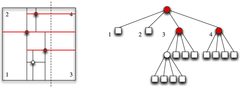
Figure 1: An example of a (point) quadtree: on the left the partition of the unit square induced by the tree data structure on the right (the children are ordered according to the numbering of the regions on the left). Answering the partial match query materialized by the dashed line on the left requires one to visit the colored nodes. Note that each one of the visited nodes correspond to a horizontal line that is crossed by the query.

Analysis of partial match retrieval. For the analysis, we will focus on the model of random quadtrees, where the data points are independent and uniformly distributed in the unit square. In the present case, the data are just points and the problem of partial match retrieval consists in reporting all the data with one of the coordinates (say the first) being $s\in[0,1]$. It is a simple observation that the number of nodes of the tree visited when performing the search is precisely $C_{n}(s)$, the number of regions in the quadtree that intersect a vertical line at $s$. The first analysis of partial match in quadtrees is due to Flajolet et al. FlGoPuRo1993 (after the pioneering work of Flajolet and Puech FlPu1986 in the case of $k$-d trees). They studied the singularities of a differential system for the generating functions of partial match cost to prove that, for a random query $\xi$, being independent of the tree and uniformly distributed on $[0,1]$, one has $\mathbf{E}[{C_{n}(\xi)}]\sim\kappa n^{\beta}$ where

$$\kappa=\frac{\Gamma(2\beta+2)}{2\Gamma(\beta+1)^{3}}\quad\mbox{and}\quad\beta=\frac{\sqrt{17}-3}{2},$$ (1)

and $\Gamma(x)$ denotes the Gamma function $\Gamma(x)=\int_{0}^{\infty}t^{x-1}e^{-t}\,dt$. Flajolet et al. FlGoPuRo1993 actually proved a more precise version of this estimate which will be crucial for us,

$$\mathbf{E}\bigl{[}C_{n}(\xi)\bigr{]}=\kappa n^{\beta}-1+O\bigl{(}n^{\beta-1}\bigr{)}.$$ (2)

(This may also be obtained from the explicit expression for $\mathbf{E}[{C_{n}(\xi)}]$ devised by Chern and Hwang ChHw2003 .)

Our aim in this paper is to gain a refined understanding of the cost beyond the level of expectations. In order to quantify the order of typical deviations from the mean, we study the order of the variance together with limit distributions. However, deriving higher moments turns out to be subtle. In particular, when the query line is random (like above) although the four subtrees at the root are independent given their sizes, the contributions of the two subtrees that do hit the query line are dependent. Indeed, the relative location of the query line inside these two subtrees is again uniform, but unfortunately it is same in both regions. Hence, one cannot easily setup recurrence relations and perform an asymptotic analysis exploiting independence. This issue has not yet been addressed appropriately, and there is currently no result on the variance or higher moments for $C_{n}(\xi)$.

Another issue lies in the definition of the cost measure itself: even if the data follow some distribution, should one assume that the query follows the same distribution? In other words, should we focus on $C_{n}(\xi)$? Maybe not. But then, what distribution should one use for the query line?

One possible approach to overcome both problems is to consider the query line to be fixed and to study $C_{n}(s)$ for $s\in[0,1]$. This raises another problem: even if $s$ is fixed at the top level, as the search is performed, the relative location of the queries in the recursive calls varies from one node to another. Thus, in following this approach, one is led to consider the entire stochastic process $(C_{n}(s))_{s\in[0,1]}$; this is the method we use here.

Recently Curien and Joseph CuJo2010 obtained some results in this direction. They proved that for every fixed $s\in(0,1)$,

$$\mathbf{E}\bigl{[}C_{n}(s)\bigr{]}\sim K_{1}\cdot h(s)n^{\beta}\qquad\mbox{with }K_{1}=\frac{\Gamma(2\beta+2)\Gamma(\beta+2)}{2\Gamma(\beta+1)^{3}\Gamma(\beta/2+1)^{2}},$$ (3)

where the function $h$ defined below will play a central role in the entire study

$$h(s):=\bigl{(}s(1-s)\bigr{)}^{\beta/2}.$$ (4)

On the other hand, Flajolet et al. FlGoPuRo1993 , FlLaLaSa1995 prove that, along the edge one has $\mathbf{E}[{C_{n}(0)}]=\Theta(n^{\sqrt{2}-1})$, so that $\mathbf{E}[{C_{n}(0)}]=o(n^{\beta})$ (see also CuJo2010 ). The behavior about the $x$-coordinate $U$ of the first data point certainly resembles that along the edge, so that one has $\mathbf{E}[{C_{n}(U)}]=o(n^{\beta})$. This suggests that $C_{n}(s)$ should not be concentrated around its mean, and that $n^{-\beta}C_{n}(s)$ should converge to a nondegenerate random variable as $n\to\infty$. Below, we confirm this and prove a functional limit law for $(n^{-\beta}C_{n}(s))_{s\in[0,1]}$ and characterize the limit process. From this we obtain refined asymptotic information on the complexity of partial match queries in quadtrees.

2 Main results and implications

We denote by $\mathcal{D}[0,1]$ the space of càdlàg functions on $[0,1]$ and by $\|f\|:=\sup_{t\in[0,1]}|f(t)|$ the uniform norm of $f\in\mathcal{D}[0,1]$. Our main contribution is to prove the following convergence result:

Theorem 1

Let $C_{n}(s)$ be the cost of a partial match query at a fixed line $s$ in a random quadtree. Then there exists a random continuous function $Z$ such that, as $n\to\infty$,

$$\biggl{(}\frac{C_{n}(s)}{K_{1}n^{\beta}},s\in[0,1]\biggr{)}\stackrel{{\scriptstyle d}}{{\rightarrow}}\bigl{(}Z(s),s\in[0,1]\bigr{)}.$$ (5)

This convergence in distribution holds in $\mathcal{D}[0,1]$ equipped with the Skorokhod topology.

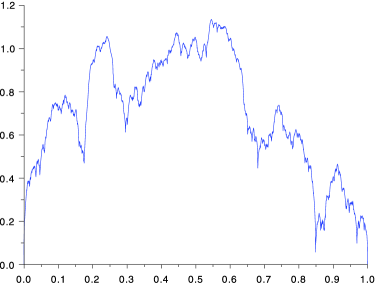
Figure 2: A simulation of the limit process $Z$.

The limit process $Z$ may be characterized as follows (see Figure 2 for a simulation):

Proposition 2.

The distribution of the random function $Z$ in (5) is a fixed point of the following functional recursive distributional equation, as process in $s\in[0,1]$:

$$Z(s) \stackrel{{\scriptstyle d}}{{=}} \mathbf{1}_{\{{s<U}\}}\biggl{[}(UV)^{\beta}Z^{(1)}\biggl{(}\frac{s}{U}\biggr{)}+\bigl{(}U(1-V)\bigr{)}^{\beta}Z^{(2)}\biggl{(}\frac{s}{U}\biggr{)}\biggr{]}$$

$${}+\mathbf{1}_{\{{s\geq U}\}}\biggl{[}\bigl{(}(1-U)V\bigr{)}^{\beta}Z^{(3)}\biggl{(}\frac{s-U}{1-U}\biggr{)}$$

$$\hskip 14.0pt\qquad\quad{}+\bigl{(}(1-U)(1-V)\bigr{)}^{\beta}Z^{(4)}\biggl{(}\frac{s-U}{1-U}\biggr{)}\biggr{]},$$

where $U$ and $V$ are independent $[0,1]$-uniform random variables and $Z^{(i)}$, $i=1,\ldots,4$ are independent copies of the process $Z$, which are also independent of $U$ and $V$. Furthermore, $Z$ in (5) is the only continuous solution of (2) with $\mathbf{E}[{\|Z\|^{2}}]<\infty$ and $\mathbf{E}[{Z(\xi)}]=\Gamma(\beta/2+1)^{2}/\Gamma(\beta+2)$ where $\xi$ is independent of $Z$ and uniformly distributed on $[0,1]$.

The methods applied to prove Theorem 1 also guarantee convergence of the variance of the costs of partial match queries. The following theorem for uniform queries $\xi$ is the direct extension of the pioneering work in FlPu1986 , FlGoPuRo1993 for the cost of partial match queries at a uniform line $\xi$ in random two-dimensional trees.

Theorem 3

If $\xi$ is uniformly distributed on $[0,1]$, independent of $(C_{n})$ and $Z$, then

$$\frac{C_{n}(\xi)}{K_{1}n^{\beta}}\to Z(\xi)$$

in distribution, as $n\to\infty$. Moreover, $\operatorname{Var}({C_{n}(\xi)})\sim K_{4}n^{2\beta}$ where $K_{4}\approx\break 0.447363034$ is given by, with $K_{1}$ in (3),

$$K_{4} := K_{1}^{2}\cdot\operatorname{Var}\bigl{(}Z(\xi)\bigr{)}$$

$$= K_{1}^{2}\biggl{(}\frac{2(2\beta+1)}{3(1-\beta)}\mathrm{B}(\beta+1,\beta+1)^{2}-\mathrm{B}(\beta/2+1,\beta/2+1)^{2}\biggr{)}.$$

Here $\mathrm{B}(a,b):=\int_{0}^{1}t^{a-1}(1-t)^{b-1}\,dt$ denotes the Eulerian integral for $a,b>-1$. In particular, Theorem 3 identifies the first-order asymptotics of$\operatorname{Var}({C_{n}(\xi)})$ which is to be compared with studies that neglected the dependence between the contributions of the subtrees mentioned above MaPaPr2001 , NeRu2001 , Neininger2000 . A refined result about the variance $\operatorname{Var}({C_{n}(s)})$ at a fixed location reads

$$\operatorname{Var}\bigl{(}C_{n}(s)\bigr{)}\sim K_{1}^{2}\operatorname{Var}\bigl{(}Z(s)\bigr{)}n^{2\beta},$$

where $s\in(0,1)$ and an explicit expression for $\operatorname{Var}({Z(s)})$ is given by

$$\operatorname{Var}\bigl{(}Z(s)\bigr{)}=K_{2}h^{2}(s)=\biggl{[}2\mathrm{B}(\beta+1,\beta+1)\frac{2\beta+1}{3(1-\beta)}-1\biggr{]}h^{2}(s).$$ (8)

Another consequence of Theorem 1 concerns the order of the cost of the worst query given by $\sup_{s\in[0,1]}C_{n}(s)$.

Theorem 4

Let $S_{n}=\sup_{s\in[0,1]}C_{n}(s)$. Then as $n\to\infty$,

$$\frac{S_{n}}{K_{1}n^{\beta}}\to S:=\sup_{s\in[0,1]}Z(s),$$

in distribution and with convergence of all moments. In particular, $\mathbf{E}[{S}]<\infty$, $\operatorname{Var}({S})<\infty$ and we have

$$\mathbf{E}[{S_{n}}]\sim K_{1}n^{\beta}\mathbf{E}[{S}]\quad\mbox{and}\quad\operatorname{Var}({S_{n}})\sim K_{1}^{2}n^{2\beta}\operatorname{Var}({S}).$$

Note that the sequence $n^{-\beta}\mathbf{E}[{S_{n}}]$ is bounded. In particular, $\mathbf{E}[{S_{n}}]$ has the same order of magnitude as the cost of a search query at any single location, and does not include any extra factor growing with $n$. Interestingly, the one-dimensional marginals of the limit process $(Z(s),s\in[0,1])$ are all the same up to a deterministic multiplicative constant given by the function $h$:

Theorem 5

There exists a random variable $\Psi\geq 0$ such that for all $s\in[0,1]$,

$$Z(s)\stackrel{{\scriptstyle d}}{{=}}h(s)\cdot\Psi.$$ (9)

The distribution of $\Psi$ is the unique solution of the fixed-point equation

$$\Psi\stackrel{{\scriptstyle d}}{{=}}U^{\beta/2}V^{\beta}\Psi+U^{\beta/2}(1-V)^{\beta}\Psi$$ (10)

with $\mathbf{E}[{\Psi}]=1$ and $\mathbf{E}[{\Psi^{2}}]<\infty$ where $\Psi^{\prime}$ is an independent copy of $\Psi$ and $(\Psi,\Psi^{\prime})$ is independent of $(U,V)$.

Convergence of all moments of the supremum $n^{-\beta}S_{n}$ in Theorem 4 implies uniform integrability of any moment of the process $n^{-\beta}C_{n}$, hence the following result about convergence of all moments.

Corollary 6.

For all $s\in[0,1]$, we have

$$\mathbf{E}\biggl{[}\biggl{(}\frac{C_{n}(s)}{K_{1}n^{\beta}}\biggr{)}^{m}\biggr{]}\rightarrow\mathbf{E}\bigl{[}Z(s)^{m}\bigr{]}=c_{m}h(s)^{m}$$

for all $m\in\mathbb{N}$ as $n\to\infty$ where $c_{m}$ is given by

$$c_{m} = \frac{\beta m+1}{(m-1)(m+1-(3/2)\beta m)}$$

$${}\times\sum_{\ell=1}^{m-1}\pmatrix{m\cr\ell}\mathrm{B}\bigl{(}\beta\ell+1,\beta(m-\ell)+1\bigr{)}c_{\ell}c_{m-\ell}$$

for $m\geq 2$ where $c_{1}=1$. An analogous result holds true for $\mathbf{E}[{C_{n}(\xi)}]$ where $\xi$ is uniform on $[0,1]$ and independent of $(C_{n})_{n\geq 0}$ and $Z$, and for moments involving queries at multiple locations.

Plan of the paper. Our approach requires to work with the process $(C_{n}(s)\dvtx s\in[0,1])$ and is based on the recursive decomposition of the tree at the root. This yields a recursive distributional recurrence for $(C_{n}(s)\dvtx s\in[0,1])$ to which we apply a functional version of the contraction method. In Section 3, we give an overview of this underlying methodology. In particular, we discuss the novel results of Neininger and Sulzbach NeSu2011a about the contraction method in function spaces which we will apply. Sections 4 and 5 are dedicated to the proofs of two of the main ingredients required to apply the results from NeSu2011a , the existence of a continuous solution of the limit recursive equation and the uniform convergence of the rescaled first moment $n^{-\beta}\mathbf{E}[{C_{n}(s)}]$ at an appropriate rate. In Section 6, we identify the variance and the supremum of the limit process $Z$ and deduce the large $n$ asymptotics for $C_{n}(s)$ in Theorems 3 and 4. Finally, we prove analogous results for the cases of $2$-d trees in Section 7. Our results on quadtrees have been announced in the extended abstract BrNeSu2011a .

3 Contraction method in function spaces

3.1 Overview of the method

The aim of this section is to give an overview of the method we employ to prove Theorem 1. It is based on a contraction argument in a certain space of probability distributions. In the context of the analysis of algorithms, the method was first employed by Rösler Roesler1991a who proved convergence in distribution for the rescaled total cost of the randomized version of quicksort. The method was then further developed by Rösler Roesler1992 , Rachev and Rüschendorf RaRu1995 , and later on in Ro01 , Ne01 , NeRu04 , NeRu04b , DrJaNe , EiRu07 and has permitted numerous analyses in distribution for random discrete structures.

So far, the method has mostly been used to analyze random variables taking real values, though a few applications on function spaces have been made; see DrJaNe , EiRu07 , GR09 . Here we are interested in the function space ${\mathcal{D}}[0,1]$ endowed with the Skorokhod topology (see, e.g., Billingsley1999 ), but the main idea persists: (1) devise a recursive equation for the quantity of interest [here the process $(C_{n}(s),s\in[0,1])$], and (2) based on a properly rescaled version of the quantity deduce a limit equation, that is, a recursive distributional equation that the limit may satisfy; (3) if the map of distributions associated to the limit equation is a contraction in a certain metric space, then a fixed point is unique and may be obtained by iteration. The contraction may also be exploited to obtain weak convergence to the fixed point. We now move on to the first step of this program.

Write $I_{1}^{(n)},\ldots,I_{4}^{(n)}$ for the number of points falling in the four regions created by the point stored at the root. Then, given the coordinates of the first data point $(U,V)$, we have (cf. Figure 1)

$$\bigl{(}I_{1}^{(n)},\ldots,I_{4}^{(n)}\bigr{)}$$

(12)

$$\qquad\stackrel{{\scriptstyle d}}{{=}}\operatorname{Mult}\bigl{(}n-1;UV,U(1-V),(1-U)(1-V),(1-U)V\bigr{)}.$$

Observe that, for the cost inside a subregion, what matters is the location of the query line relative to the region. Thus a decomposition at the root yields the following recursive relation for any $n\geq 1$:

$$C_{n}(s) \stackrel{{\scriptstyle d}}{{=}} 1+\mathbf{1}_{\{{s<U}\}}\biggl{[}C^{(1)}_{I_{1}^{(n)}}\biggl{(}\frac{s}{U}\biggr{)}+C^{(2)}_{I_{2}^{(n)}}\biggl{(}{\frac{s}{U}}\biggr{)}\biggr{]}$$

$${}+\mathbf{1}_{\{{s\geq U}\}}\biggl{[}C^{(3)}_{I_{3}^{(n)}}\biggl{(}\frac{1-s}{1-U}\biggr{)}+C^{(4)}_{I_{4}^{(n)}}\biggl{(}\frac{1-s}{1-U}\biggr{)}\biggr{]},$$

where $U,I_{1}^{(n)},\ldots,I_{4}^{(n)}$ are the quantities already introduced and $(C^{(1)}_{k}),\ldots,\break(C^{(4)}_{k})$ are independent copies of the sequence $(C_{k},k\geq 0)$, independent of $(U,V,I_{1}^{(n)},\ldots,I_{4}^{(n)})$. We stress that this equation does not only hold true pointwise for fixed $s$ but also as càdlàg functions on the unit interval. The relation in (3.1) is the fundamental equation for us.

Letting $n\to\infty$ (formally) in (3.1) suggests that if $n^{-\beta}C_{n}(s)$ does converge to a random variable $Z(s)$ in a sense to be made precise, then the distribution of the process $(Z(s),0\leq s\leq 1)$ should satisfy the following fixed point equation:

$$Z(s) \stackrel{{\scriptstyle d}}{{=}} \mathbf{1}_{\{{s<U}\}}\biggl{[}(UV)^{\beta}Z^{(1)}\biggl{(}\frac{s}{U}\biggr{)}+\bigl{(}U(1-V)\bigr{)}^{\beta}Z^{(2)}\biggl{(}\frac{s}{U}\biggr{)}\biggr{]}$$

$${}+\mathbf{1}_{\{{s\geq U}\}}\biggl{[}\bigl{(}(1-U)V\bigr{)}^{\beta}Z^{(3)}\biggl{(}\frac{s-U}{1-U}\biggr{)}$$

$$\hskip 25.0pt\qquad{}+\bigl{(}(1-U)(1-V)\bigr{)}^{\beta}Z^{(4)}\biggl{(}\frac{s-U}{1-U}\biggr{)}\biggr{]},$$

where $U$ and $V$ are independent $[0,1]$-uniform random variables and $Z^{(i)}$, $i=1,\ldots,4$ are independent copies of the process $Z$, which are also independent of $U$ and $V$.

The last step leading to the fixed point equation (3.1) needs now to be made rigorous. It is at this point that the contraction method enters the game. The distribution of a solution to our fixed-point equation (3.1) lies in the set of probability measures on the Polish space $(\mathcal{D}[0,1],d)$, which is the set we have to endow with a suitable metric. Here, $d$ denotes the Skorokhod metric; see, for example, Billingsley1999 .

The recursive equation (3.1) is an example for the following, more general setting of random additive recurrences: Let $(X_{n})$ be $\mathcal{D}[0,1]$-valued random variables with

$$X_{n}\stackrel{{\scriptstyle d}}{{=}}\sum_{r=1}^{K}A_{r}^{(n)}\bigl{(}X_{I_{r}^{(n)}}^{(r)}\bigr{)}+b^{(n)},\qquad n\geq 1,$$ (15)

where $(A_{1}^{(n)},\ldots,A_{K}^{(n)})$ are random continuous linear operators on $\mathcal{D}[0,1]$, $b^{(n)}$ is a $\mathcal{D}[0,1]$-valued random variable, $I_{1}^{(n)},\ldots,I_{K}^{(n)}$ are random integers between $0$ and $n-1$ and the sequences of process $(X_{n}^{(1)})$, …, $(X_{n}^{(K)})$ are distributed like $(X_{n})$. Moreover $(A_{1}^{(n)},\ldots,A_{K}^{(n)},b^{(n)},I_{1}^{(n)},\ldots,I_{K}^{(n)})$,$(X_{n}^{(1)}),\ldots,(X_{n}^{(K)})$ are independent.

At this point, one should comment on the term random continuous linear operator: As explained explicitly in NeSu2011a , $A$ is a random continuous linear operator on $\mathcal{D}[0,1]$, if it takes values in the set of endomorphisms on $\mathcal{D}[0,1]$ that are both continuous with respect to the supremum norm and to the Skorokhod metric. Moreover, for any $f\in\mathcal{D}[0,1]$ and $t\in[0,1]$, the quantity $Af(t)$ has to be a real-valued random variable, and the same is assumed for $\|A\|_{\mathrm{op}}$ (see below for the definition). Finally, we remember that convergence $d(f_{n},f)\rightarrow 0$ in the Skorokhod metric means that there exists a sequence of monotonically increasing bijections $(\lambda_{n})$ on the unit interval such that $f_{n}(\lambda_{n}(t))\rightarrow f(t)$ and $\lambda_{n}(t)\rightarrow t$ both uniformly in $t$ as $n\rightarrow\infty$.

To establish Theorem 1 as a special case of this setting, we use Proposition 7 below. Proposition 7 is part of the main convergence theorem in Neininger and Sulzbach NeSu2011a . We first state conditions needed to deal with the general recurrence (15); we will then justify that it can indeed be used in the case of cost of partial match queries. Consider the following assumptions, where, for a random variable $X$ in $\mathcal{D}[0,1]$ we write $\|X\|_{2}:=\mathbf{E}[{\|X\|^{2}}]^{1/2}$, for a linear operator $A$ we write $\|A\|_{2}:=\mathbf{E}[{\|A\|_{\mathrm{op}}^{2}}]^{1/2}$ with $\|A\|_{\mathrm{op}}:=\sup_{\|x\|=1}\|A(x)\|$. Suppose $(X_{n})$ obeys (15) and the following:[(A3)]

Convergence and contraction. We have $\|A_{r}^{(n)}\|_{2},\|b^{(n)}\|_{2}<\infty$ for all $r=1,\ldots,K$ and $n\geq 0$ and there exist random continuous linear operators $A_{1},\ldots,A_{K}$ on $\mathcal{D}[0,1]$ and a $\mathcal{D}[0,1]$-valued random variable $b$ such that, for some positive sequence $R(n)\downarrow 0$, as $n\to\infty$,

$$\bigl{\|}b^{(n)}-b\bigr{\|}_{2}+\sum_{r=1}^{K}\bigl{\|}A_{r}^{(n)}-A_{r}\bigr{\|}_{2}=O\bigl{(}R(n)\bigr{)}$$ (16)

and for all $\ell\in\mathbb{N}$,

$$\mathbf{E}\bigl{[}\mathbf{1}_{\{I^{(n)}_{r}\in\{0,\ldots,\ell\}\}}\bigl{\|}A^{(n)}_{r}\bigr{\|}_{\mathrm{op}}^{2}\bigr{]}\to 0$$

and

$$L^{*}=\limsup_{n\rightarrow\infty}\mathbf{E}\Biggl{[}\sum_{r=1}^{K}\bigl{\|}A_{r}^{(n)}\bigr{\|}_{\mathrm{op}}^{2}\frac{R(I_{r}^{(n)})}{R(n)}\Biggr{]}<1.$$ (17)

Existence and equality of moments. $\mathbf{E}[{\|X_{n}\|^{2}}]<\infty$ for all $n$ and $\mathbf{E}[{X_{n_{1}}(t)}]=\mathbf{E}[{X_{n_{2}}(t)}]$ for all $n_{1},n_{2}\in\mathbb{N}_{0},t\in[0,1]$.

Existence of a continuous solution. There exists a solution $X$ of the fixed-point equation

$$X\stackrel{{\scriptstyle d}}{{=}}\sum_{r=1}^{K}A_{r}\bigl{(}X^{(r)}\bigr{)}+b$$ (18)

with continuous paths, $\mathbf{E}[{\|X\|^{2}}]<\infty$ and $\mathbf{E}[{X(t)}]=\mathbf{E}[{X_{1}(t)}]$ for all $t\in[0,1]$. Again the random variables $(A_{1},\ldots,A_{K},b),X^{(1)},\ldots,X^{(K)}$ are independent and $X^{(1)},\ldots,X^{(K)}$ are distributed like $X$.

Perturbation condition. $X_{n}=W_{n}+h_{n}$ where $\|h_{n}-h\|\to 0$ with $h\in\mathcal{C}[0,1]$ and random variables $W_{n}$ in $\mathcal{D}[0,1]$ such that there exists a sequence $(r_{n})$ with, as $n\to\infty$,

$$\mathbf{P}\bigl{(}W_{n}\notin\mathcal{D}_{r_{n}}[0,1]\bigr{)}\to 0.$$

Here, $\mathcal{D}_{r_{n}}[0,1]\subset\mathcal{D}[0,1]$ denotes the set of functions on the unit interval continuous at $1$, for which there is a decomposition of $[0,1]$ into intervals of length as least $r_{n}$ on which they are constant.

Rate of convergence. $R(n)=o(\log^{-2}(1/r_{n}))$.

The contraction method presented here for the space $(\mathcal{D}[0,1],d)$ is based on the Zolotarev metric $\zeta_{2}$; see NeSu2011a . We state the part of the main convergence theorem of Neininger and Sulzbach NeSu2011a that we will use. In the next section, we will prove our main result, Theorem 1, with the help of Proposition 7.

Proposition 7.

Let $(X_{n})$ fulfill (15). Provided that assumptions (A1)–(A3) are satisfied, the solution $X$ of the fixed-point equation (18) is unique. [(iii)]

For all $t\in[0,1]$, $X_{n}(t)\to X(t)$ in distribution, with convergence of the first two moments.

If $\xi$ is independent of $(X_{n}),X$ and distributed on $[0,1]$, then $X_{n}(\xi)\to X(\xi)$ in distribution again with convergence of the first two moments.

If also (A4) and (A5) hold, then $X_{n}\rightarrow X$ in distribution in $(\mathcal{D}[0,1],d)$.

Note that $X_{n}\rightarrow X$ in distribution in $(\mathcal{D}[0,1],d)$ with $X$ having continuous sample paths implies that we can find versions of $(X_{n}),X$ on a suitable probability space such that $\|X_{n}-X\|\rightarrow 0$ almost surely. However, in general we do not have $X_{n}\rightarrow X$ in distribution in $\mathcal{D}[0,1]$ endowed with the uniform topology due to problems with measurability; see Billingsley1999 , Section 15 and NeSu2011a , Section 2.2.

3.2 The functional limit theorem: Proof of Theorem 1

The aim of this section is to prove Theorem 1 with the help of Proposition 7 from Neininger and Sulzbach NeSu2011a . More precisely, in the following we prove conditions (A1)–(A5), except two which require much more work: the existence of a continuous solution (A3), and the uniform convergence of the mean in (A1) are treated separately in Sections 4 and 5, respectively.

Following the heuristics in the Introduction we scale the additive recurrence (3.1) by $n^{\beta}$. Let $Q_{0}(t):=0$ and

$$Q_{n}(t)=\frac{C_{n}(t)}{K_{1}n^{\beta}},\qquad n\geq 1.$$

The recursive distributional equation then rewrites in terms of $Q_{n}$ as

$$\bigl{(}Q_{n}(t)\bigr{)}_{t\in[0,1]}$$

$$\qquad\stackrel{{\scriptstyle{d}}}{{=}}\biggl{(}\mathbf{1}_{\{{t<U}\}}\biggl{[}\biggl{(}\frac{I_{1}^{(n)}}{n}\biggr{)}^{\beta}Q_{I_{1}^{(n)}}^{(1)}\biggl{(}\frac{t}{U}\biggr{)}+\biggl{(}\frac{I_{2}^{(n)}}{n}\biggr{)}^{\beta}Q_{I_{2}^{(n)}}^{(2)}\biggl{(}\frac{t}{U}\biggr{)}\biggr{]}$$

(19)

$$\quad\qquad\hskip 6.0pt{}+\mathbf{1}_{\{{t\geq U}\}}\biggl{[}\biggl{(}\frac{I_{3}^{(n)}}{n}\biggr{)}^{\beta}Q_{I_{3}^{(n)}}^{(3)}\biggl{(}\frac{t-U}{1-U}\biggr{)}+\biggl{(}\frac{I_{4}^{(n)}}{n}\biggr{)}^{\beta}Q_{I_{4}^{(n)}}^{(4)}\biggl{(}\frac{t-U}{1-U}\biggr{)}\biggr{]}$$

$$\hskip 188.0pt\quad\qquad\hskip 30.0pt\qquad{}+\frac{1}{K_{1}n^{\beta}}\biggr{)}_{t\in[0,1]},$$

where $U,I_{1}^{(n)},\ldots,I_{4}^{(n)}$ are the quantities already introduced in Section 3.1 and (3.1) and $(Q^{(1)}_{n})_{n\geq 0},\ldots,(Q^{(4)}_{n})_{n\geq 0}$ are independent copies of $(Q_{n})_{n\geq 0}$, independent of $(U,V,I_{1}^{(n)},\ldots,I_{4}^{(n)})$. The convergence of the coefficients $(I_{j}^{(n)}/n)^{\beta}$ suggests that a limit of $Q_{n}(t)$ should satisfy the fixed-point equation (3.1).

The recurrence relation. Most details consist in setting the right form of the recurrence relation: for (A2) to be satisfied, we need to use a scaling that leads to an expectation which is independent of $n$. This is not the case for $Q_{n}(t)$. Denoting $\mu_{n}(t)=\mathbf{E}[{C_{n}(t)}]$, we are naturally led to consider $Y_{0}(t):=0$ and

$$Y_{n}(t)=\frac{C_{n}(t)-\mu_{n}(t)}{K_{1}n^{\beta}}=Q_{n}(t)-h(t)+O\bigl{(}n^{-\varepsilon}\bigr{)},\qquad n\geq 1,$$

where the error term is deterministic and uniform in $t\in[0,1]$. Hence it is sufficient to prove convergence of the sequence $(Y_{n})_{n\geq 1}$. The distributional recursion in terms of $Y_{n}$ is

$$\bigl{(}Y_{n}(t)\bigr{)}_{t\in[0,1]}$$

$$\qquad\stackrel{{\scriptstyle{d}}}{{=}}\biggl{(}\mathbf{1}_{\{{t<U}\}}\biggl{[}\biggl{(}\frac{I_{1}^{(n)}}{n}\biggr{)}^{\beta}Y_{I_{1}^{(n)}}^{(1)}\biggl{(}\frac{t}{U}\biggr{)}+\biggl{(}\frac{I_{2}^{(n)}}{n}\biggr{)}^{\beta}Y_{I_{2}^{(n)}}^{(2)}\biggl{(}\frac{t}{U}\biggr{)}\biggr{]}$$

$$\qquad\quad\hskip 6.0pt{}+\mathbf{1}_{\{{t\geq U}\}}\biggl{[}\biggl{(}\frac{I_{3}^{(n)}}{n}\biggr{)}^{\beta}Y_{I_{3}^{(n)}}^{(3)}\biggl{(}\frac{t-U}{1-U}\biggr{)}+\biggl{(}\frac{I_{4}^{(n)}}{n}\biggr{)}^{\beta}Y_{I_{4}^{(n)}}^{(4)}\biggl{(}\frac{t-U}{1-U}\biggr{)}\biggr{]}$$

$$\qquad\quad\hskip 6.0pt{}+\mathbf{1}_{\{{t<U}\}}\biggl{[}\frac{\mu_{I_{1}^{(n)}}({t}/{U})+\mu_{I_{2}^{(n)}}({t}/{U})}{K_{1}n^{\beta}}\biggr{]}$$

$$\qquad\quad\hskip 6.0pt{}+\mathbf{1}_{\{{t\geq U}\}}\biggl{[}\frac{\mu_{I_{3}^{(n)}}({(t-U)}/{(1-U)})+\mu_{I_{4}^{(n)}}({(t-U)}/{(1-U)})}{K_{1}n^{\beta}}\biggr{]}$$

$$\hskip 223.0pt\qquad\quad{}+\frac{1-\mu_{n}(t)}{K_{1}n^{\beta}}\biggr{)}_{t\in[0,1]},$$

where $(Y_{n}^{(1)})_{n\geq 0},\ldots,(Y_{n}^{(4)})_{n\geq 0}$ are independent copies of $(Y_{n})_{n\geq 0}$ which are also independent of the vector $(U,V,I_{1}^{(n)},\ldots,I_{4}^{(n)})$. Therefore, any possible limit $Y$ of $Y_{n}$ should satisfy the following distributional fixed-point equation:

$$\bigl{(}Y(t)\bigr{)}_{t\in[0,1]}$$

$$\qquad\stackrel{{\scriptstyle{d}}}{{=}}\biggl{(}\mathbf{1}_{\{{t<U}\}}\biggl{[}(UV)^{\beta}Y^{(1)}\biggl{(}\frac{t}{U}\biggr{)}+\bigl{(}U(1-V)\bigr{)}^{\beta}Y^{(2)}\biggl{(}\frac{t}{U}\biggr{)}\biggr{]}$$

$$\qquad\quad\hskip 1.0pt{}+\mathbf{1}_{\{{t\geq U}\}}\biggl{[}\bigl{(}(1-U)V\bigr{)}^{\beta}Y^{(3)}\biggl{(}\frac{t-U}{1-U}\biggr{)}$$

(20)

$$\qquad\quad\hskip 22.0pt\qquad{}+\bigl{(}(1-U)(1-V)\bigr{)}^{\beta}Y^{(4)}\biggl{(}\frac{t-U}{1-U}\biggr{)}\biggr{]}$$

$$\qquad\quad\hskip 1.0pt{}+\mathbf{1}_{\{{t\geq U}\}}h\biggl{(}\frac{t-U}{1-U}\biggr{)}\bigl{(}\bigl{(}(1-U)V\bigr{)}^{\beta}+\bigl{(}(1-U)(1-V)\bigr{)}^{\beta}\bigr{)}-h(t)$$

$$\qquad\quad\hskip 103.0pt{}+\mathbf{1}_{\{{t<U}\}}h\biggl{(}\frac{t}{U}\biggr{)}\bigl{(}(UV)^{\beta}+\bigl{(}U(1-V)\bigr{)}^{\beta}\bigr{)}\biggr{)}_{t\in[0,1]}.$$

Having Proposition 7 in mind, we define (random) operators $A_{r}^{(n)}$, $r=1,2,3,4$, by

$$A_{r}^{(n)}(f)(t)=\cases{\displaystyle\mathbf{1}_{\{{t<U}\}}\biggl{(}\frac{I_{r}^{(n)}}{n}\biggr{)}^{\beta}f\biggl{(}\frac{t}{U}\biggr{)},&\quad$\mbox{if }r=1,2$,\vspace*{2pt}\cr\displaystyle\mathbf{1}_{\{{t\geq U}\}}\biggl{(}\frac{I_{r}^{(n)}}{n}\biggr{)}^{\beta}f\biggl{(}\frac{t-U}{1-U}\biggr{)},&\quad$\mbox{if }r=3,4.$}$$

Furthermore let $b^{(n)}(t)=\sum_{r=1}^{4}b^{(n)}_{r}(t)+(1-\mu_{n}(t))/(K_{1}n^{\beta})$ with

$$b^{(n)}_{r}(t)=\cases{\displaystyle\mathbf{1}_{\{{t<U}\}}\cdot\frac{\mu_{I_{r}^{(n)}}({t}/{U})}{K_{1}n^{\beta}},&\quad$\mbox{if }r=1,2,$\vspace*{2pt}\cr\displaystyle\mathbf{1}_{\{{t\geq U}\}}\cdot\frac{\mu_{I_{r}^{(n)}}({(t-U)}/{(1-U)})}{K_{1}n^{\beta}},&\quad$\mbox{if }r=3,4.$}$$

Then the finite-$n$ version of the recurrence relation for $(Y_{n})_{n\geq 0}$ is precisely of the form of (15).

We define similarly the coefficients of the limit recursive equation (3.2). We will then show that with these definitions, assumptions (A1)–(A5) are satisfied (again, except the existence of a continuous limit solution and the uniform convergence for the mean treated in Section 4 and 5). The operators $A_{1},\ldots,A_{4}$ are defined by

$$A_{1}(f)(t) = \mathbf{1}_{\{{t<U}\}}(UV)^{\beta}f\biggl{(}\frac{t}{U}\biggr{)},$$

$$A_{2}(f)(t) = \mathbf{1}_{\{{t<U}\}}\bigl{(}U(1-V)\bigr{)}^{\beta}f\biggl{(}\frac{t}{U}\biggr{)},$$

$$A_{3}(f)(t) = \mathbf{1}_{\{{t\geq U}\}}\bigl{(}(1-U)V\bigr{)}^{\beta}f\biggl{(}\frac{t-U}{1-U}\biggr{)},$$

$$A_{4}(f)(t) = \mathbf{1}_{\{{t\geq U}\}}\bigl{(}(1-U)(1-V)\bigr{)}^{\beta}f\biggl{(}\frac{t}{U}\biggr{)}$$

and $b(t)=\sum_{r=1}^{4}b_{r}(t)-h(t)$ with

$$b_{1}(t) = \mathbf{1}_{\{{t<U}\}}(UV)^{\beta}h\biggl{(}\frac{t}{U}\biggr{)},$$

$$b_{2}(t) = \mathbf{1}_{\{{t<U}\}}\bigl{(}U(1-V)\bigr{)}^{\beta}h\biggl{(}\frac{t}{U}\biggr{)},$$

$$b_{3}(t) = \mathbf{1}_{\{{t\geq U}\}}\bigl{(}(1-U)V\bigr{)}^{\beta}h\biggl{(}\frac{t-U}{1-U}\biggr{)},$$

$$b_{4}(t) = \mathbf{1}_{\{{t\geq U}\}}\bigl{(}(1-U)(1-V)\bigr{)}^{\beta}h\biggl{(}\frac{t}{U}\biggr{)}.$$

The operators $A_{1},\ldots,A_{4},A_{1}^{(n)},\ldots,A_{4}^{(n)}$ are linear for each $n$. Moreover, they are bounded above by one, which implies that they are norm-continuous. Their norm functions are real-valued random variables. In order to establish that they are indeed random continuous linear operators on $(\mathcal{D}[0,1],d)$ it remains to check that they are continuous with respect to the Skorokhod topology. To this end, it is sufficient to prove that

$$d(f_{n},f)\rightarrow 0\quad\Rightarrow\quad d\biggl{(}\mathbf{1}_{\{{t<u}\}}f_{n}\biggl{(}\frac{t}{u}\biggr{)},\mathbf{1}_{\{{t<u}\}}f\biggl{(}\frac{t}{u}\biggr{)}\biggr{)}\rightarrow 0$$

for any $u\in[0,1]$. This follows easily since $\|f_{n}(\lambda_{n}(t))-f(t)\|\rightarrow 0$ with monotonically increasing bijections $\lambda_{n}$ on the unit interval such that $\|\lambda_{n}(t)-t\|\rightarrow 0$ implies $\|\mathbf{1}_{\{{\beta_{n}(t)<u}\}}f_{n}(\beta_{n}(t)/u)-\mathbf{1}_{\{{t<u}\}}f(t/u)\|\rightarrow 0$ where $\beta_{n}(t)=u\lambda_{n}(t/u)$ for $t\leq u$ and $\beta_{n}(t)=t$ for $t>u$.

We are now ready to check that assumptions (A1)–(A5) indeed hold, taking the results of Sections 4 and 5 for granted.

(A3) Existence of a continuous solution. In Section 4, we construct a continuous solution $Z$ of the fixed-point equation (3.1) with $\mathbf{E}[{\|Z\|^{2}}]<\infty$ and $\mathbf{E}[{Z(t)}]=h(t)=(t(1-t))^{\beta/2}$. Hence the function $Y(t)=Z(t)-h(t)$ is a continuous solution of (3.2) with $\mathbf{E}[{Y(t)}]=0$ and $\mathbf{E}[{\|Y\|^{2}}]<\infty$. A direct computation shows that $\mathbf{E}[{\|A_{r}\|_{\mathrm{op}}^{2}}]=\mathbf{E}[{(UV)^{2\beta}}]=(2\beta+1)^{-2}$, for $r=1,\ldots,4$. Observe that

$$L:=\sum_{r=1}^{4}\mathbf{E}\bigl{[}\|A_{r}\|_{\mathrm{op}}^{2}\bigr{]}=\frac{4}{(2\beta+1)^{2}}<1.$$

In particular, $Y$ is the unique solution of (3.2) with $\mathbf{E}[{Y(t)}]=0$ and $\mathbf{E}[{\|Y\|^{2}}]<\infty$. Thus, $Z$ is the unique solution of (2) with $\mathbf{E}[{Z(t)}]=h(t)$ and $\mathbf{E}[{\|Z\|^{2}}]<\infty$. By the arguments in CuJo2010 , Section 5, the mean function of any process with càdlàg paths and finite moments satisfying (2) is a multiple of $h(s)$. Hence, we may replace the condition $\mathbf{E}[{Z(t)}]=h(t)$ by $\mathbf{E}[{Z(\xi)}]=\Gamma(\beta/2+1)^{2}/\Gamma(\beta+2)$ as formulated in Proposition 2.

(A2) Existence and equality of moments. The precise scaling we chose ensures that $\mathbf{E}[{Y_{n}(t)}]=0$, for all $n\geq 1$ and $t\in[0,1]$. The second moments $\mathbf{E}[{\|Y_{n}\|^{2}}]$ are finite as the random variables $\|Y_{n}\|$ are bounded for every fixed $n$.

(A1) Convergence and contraction. It suffices to focus on the terms

$$\bigl{\|}A_{1}^{(n)}-A_{1}\bigr{\|}_{2}\quad\mbox{and}\quad\bigl{\|}b^{(n)}_{1}-b_{1}\bigr{\|}_{2},$$

and the remaining terms can obviously be treated in the same way. Establishing the convergence only boils down to verifying that a binomial random variable Bin$(n,p)$ is properly approximated by $np$. Using the Chernoff–Hoeffding inequality for binomials Hoeffding1963 , one easily verifies that for every $\alpha>0$,

$$\mathbf{E}\biggl{[}\biggl{|}\frac{\operatorname{Bin}(n,p)}{n}-p\biggr{|}^{\alpha}\biggr{]}=O\bigl{(}n^{-\alpha/2}\bigr{)},$$ (21)

uniformly in $p\in[0,1]$. Thus, since $|x^{\beta}-y^{\beta}|\leq|x-y|^{\beta}$ for any $x,y\in[0,1]$, we have

$$\bigl{\|}A_{1}^{(n)}-A_{1}\bigr{\|}_{2}\leq\biggl{\|}\biggl{(}\frac{I_{r}^{(n)}}{n}\biggr{)}^{\beta}-(UV)^{\beta}\biggr{\|}_{2}=O\bigl{(}n^{-1/2}\bigr{)}.$$ (22)

By Proposition 12 we have $\mu_{n}(t)=K_{1}h(t)n^{\beta}+O(n^{\beta-\varepsilon})$ uniformly in $t\in[0,1]$. Therefore

$$\bigl{\|}b_{1}^{(n)}-b_{1}\bigr{\|}_{2}\leq\biggl{\|}\mathbf{1}_{\{{t<U}\}}h\biggl{(}\frac{t}{U}\biggr{)}\biggl{(}\biggl{(}\frac{I_{r}^{(n)}}{n}\biggr{)}^{\beta}-(UV)^{\beta}\biggr{)}\biggr{\|}_{2}+C\biggl{\|}\frac{(I_{1}^{(n)})^{\beta-\varepsilon}}{n^{\beta}}\biggr{\|}_{2}$$

for some constant $C>0$. Since $h$ is bounded, the first summand is $O(n^{-1/2})$ just like in (22) above. The second term is trivially bounded by $Cn^{-\varepsilon}$. Overall, we have $\|b_{1}^{(n)}-b_{1}\|_{2}=O(n^{-\varepsilon})$. Hence, since the coefficients $A_{r}^{(n)}$ are bounded by one in the operator norm and by distributional properties of $I_{1}^{(n)},\ldots,I_{4}^{(n)}$, the first two constraints in assumption (A1) are satisfied with $R(n)=Cn^{-\varepsilon}$ for a suitable constant $C>0$, and $\varepsilon>0$ may still be chosen as small as we want.

Next, we consider $L^{*}$ in (A1). By dominated convergence we have

$$L^{*}=4\mathbf{E}\bigl{[}(UV)^{2\beta}(UV)^{-\varepsilon}\bigr{]}=\frac{4}{(2\beta-\varepsilon+1)^{2}}<1$$

for $\varepsilon>0$ sufficiently small. This completes the verification of (A1).

(A4) Perturbation condition. Note that $Q_{n}$ is piecewise constant: $Q_{n}(t)=Q_{n}(s)$ for all $s,t$ if no $x$-coordinate of the first $n$ points lies between $s$ and $t$. There are $n$ independent points, the probability that there exist two lying within $n^{-3}$ of each other is at most $n^{-1}$. So (A4) is satisfied with $r_{n}=n^{-3}$.

(A5) Rate of convergence. With $r_{n}=n^{-3}$ and $R_{n}=Cn^{-\varepsilon}$, we have $R_{n}=o(\log^{-2}n)=o(\log^{-2}(1/r_{n}))$. Therefore, the condition on the rate of convergence is satisfied.

4 The limit process

In this section, we prove the existence of a process $Z\in\mathcal{C}[0,1]$, the space of continuous functions from $[0,1]$ into $\mathbb{R}$, that satisfies the distributional fixed point equation (3.1) and whose mean matches the mean of the rescaled version $Y_{n}(s)$ of $C_{n}(s)$. We construct the process $Z$ as the point-wise limit of martingales. We then show that the convergence is actually almost surely uniform, which allows us to conclude that $Z\in\mathcal{C}[0,1]$ with probability one. Figure 2 shows a simulation of the process $Z$.

We identify the nodes of the infinite quaternary tree with the set of finite words on the alphabet $\{1,2,3,4\}$,

$$\mathcal{T}=\bigcup_{n\geq 0}\{1,2,3,4\}^{n}.$$

For a node $u\in\mathcal{T}$, we write $|u|$ for its depth, that is, the distance between $u$ and the root $\varnothing$. The descendants of $u\in\mathcal{T}$ correspond to all the words in $\mathcal{T}$ with prefix $u$; in particular, the children of $u$ are $u1,\ldots,u4$. Let $\{U_{v},v\in\mathcal{T}\}$ and $\{V_{v},v\in\mathcal{T}\}$ be two independent families of i.i.d. $[0,1]$-uniform random variables. By $\mathcal{C}_{0}[0,1]$ we denote the set of continuous functions on the unit interval vanishing at the boundary, that is, $f(0)=f(1)=0$ for $f\in\mathcal{C}_{0}[0,1].$ Define the continuous operator $G\dvtx(0,1)^{2}\times\mathcal{C}_{0}[0,1]^{4}\to\mathcal{C}_{0}[0,1]$ by

$$G(x,y,f_{1},f_{2},f_{3},f_{4})(s)$$

$$\qquad=\mathbf{1}_{\{{s<x}\}}\biggl{[}(xy)^{\beta}f_{1}\biggl{(}\frac{s}{x}\biggr{)}+\bigl{(}x(1-y)\bigr{)}^{\beta}f_{2}\biggl{(}\frac{s}{x}\biggr{)}\biggr{]}$$ (23)

$$\qquad\quad{}+\mathbf{1}_{\{{s\geq x}\}}\biggl{[}\bigl{(}(1-x)y\bigr{)}^{\beta}f_{3}\biggl{(}\frac{s-x}{1-x}\biggr{)}+\bigl{(}(1-x)(1-y)\bigr{)}^{\beta}f_{4}\biggl{(}\frac{s-x}{1-x}\biggr{)}\biggr{]}.$$

Recall the definition of $h$ in (4). For every node $u\in\mathcal{T}$, let $Z_{0}^{u}=h$. Then define recursively

$$Z_{n+1}^{u}=G\bigl{(}U_{u},V_{u},Z_{n}^{u1},Z_{n}^{u2},Z_{n}^{u3},Z_{n}^{u4}\bigr{)}.$$ (24)

Finally, define $Z_{n}=Z_{n}^{\varnothing}$ to be the value observed at the root of $\mathcal{T}$ when the iteration has been started with $h$ in all the nodes at level $n$. We will see that for every $s\in[0,1]$, the sequence $(Z_{n}(s),n\geq 0)$ is a nonnegative discrete time martingale; so it converges with probability one to a finite limit.

It will be convenient to have an explicit representation for $Z_{n}$. For $s\in[0,1]$, $Z_{n}(s)$ is the sum of exactly $2^{n}$ terms, each one being the contribution of one of the boxes at level $n$ that is cut by the line at $s$. Let $\{Q_{i}^{n}(s),1\leq i\leq 2^{n}\}$ be the set of rectangles at level $n$ whose first coordinate intersect $s$. Suppose that the projection of $Q_{i}^{n}(s)$ on the first coordinate yields the interval $[\ell_{i}^{n},r_{i}^{n}]$. Then

$$Z_{n}(s)=\sum_{i=1}^{2^{n}}\operatorname{Leb}\bigl{(}Q_{i}^{n}(s)\bigr{)}^{\beta}\cdot h\biggl{(}\frac{s-\ell_{i}^{n}}{r_{i}^{n}-\ell_{i}^{n}}\biggr{)},$$ (25)

where $\operatorname{Leb}(Q_{i}^{n}(s))$ denotes the volume of the rectangle $Q_{i}^{n}(s)$. The difference between $Z_{n}$ and $Z_{n+1}$ only relies in what happens inside the boxes $Q_{i}^{n}(s)$: We have

$$Z_{n+1}(s)-Z_{n}(s)$$

(26)

$$\qquad=\sum_{i=1}^{2^{n}}\operatorname{Leb}\bigl{(}Q_{i}^{n}(s)\bigr{)}^{\beta}\cdot\biggl{[}G\bigl{(}U_{i}^{\prime},V_{i}^{\prime},h,h,h,h\bigr{)}\biggl{(}\frac{s-\ell_{i}^{n}}{r_{i}^{n}-\ell_{i}^{n}}\biggr{)}-h\biggl{(}\frac{s-\ell_{i}^{n}}{r_{i}^{n}-\ell_{i}^{n}}\biggr{)}\biggr{]},$$

where $U^{\prime}_{i},V^{\prime}_{i}$, $1\leq i\leq 2^{n}$ are i.i.d. $[0,1]$-uniform random variables. In fact, $U_{i}^{\prime}$ and $V_{i}^{\prime}$ are some of the variables $U_{u},V_{u}$ for nodes $u$ at level $n$. Observe that, although the area $\operatorname{Leb}(Q_{i}^{n}(s))$ is not a product of $n$ independent terms of the form $UV$ because of size-biasing, but $U^{\prime}_{i},V^{\prime}_{i}$ are in fact unbiased, that is, uniform. Let $\mathscr{F}_{n}$ denote the $\sigma$-algebra generated by $\{U_{u},V_{u}\dvtx|u|<n\}$. Then the family $\{U_{i}^{\prime},V_{i}^{\prime}\dvtx 1\leq i\leq 2^{n}\}$ is independent of $\mathscr{F}_{n}$.

So, to prove that $Z_{n}(s)$ is a martingale, it suffices to prove that, for $1\leq i\leq 2^{n}$,

$${\mathbf{E}\biggl{[}G\bigl{(}U_{i}^{\prime},V_{i}^{\prime},h,h,h,h\bigr{)}\biggl{(}\frac{s-\ell_{i}^{n}}{r_{i}^{n}-\ell_{i}^{n}}\biggr{)}\Big{|}\mathscr{F}_{n}\biggr{]}}=h\biggl{(}\frac{s-\ell_{i}^{n}}{r_{i}^{n}-\ell_{i}^{n}}\biggr{)}.$$

Since $U_{i}^{\prime},V_{i}^{\prime},1\leq i\leq 2^{n}$ are independent of $\mathscr{F}_{n}$, this clearly reduces to the following lemma.

Lemma 8.

For the operator $G$ defined in (4) and $U,V$ two independent $[0,1]$-uniform random variables and any $s\in[0,1]$, we have

$$\mathbf{E}\bigl{[}G(U,V,h,h,h,h)(s)\bigr{]}=h(s).$$

Since $V$ and $1-V$ have the same distribution, we have

$$\mathbf{E}\bigl{[}G(U,V,h,h,h,h)(s)\bigr{]} = 2\mathbf{E}\biggl{[}\mathbf{1}_{\{{s<U}\}}(UV)^{\beta}h\biggl{(}\frac{s}{U}\biggr{)}\biggr{]}$$

$${}+2\mathbf{E}\biggl{[}\mathbf{1}_{\{{s\geq U}\}}\bigl{(}(1-U)V\bigr{)}^{\beta}h\biggl{(}\frac{1-s}{1-U}\biggr{)}\biggr{]}.$$

Similarly, since $U$ and $1-U$ are both uniform, we clearly have

$$\mathbf{E}\bigl{[}G(U,V,h,h,h,h)(s)\bigr{]}=f(s)+f(1-s),$$

where we wrote $f(s)=2\mathbf{E}[{\mathbf{1}_{\{{s<U}\}}(UV)^{\beta}h(s/U)}]$. To complete the proof, it suffices to compute $f(s)$. We have

$$f(s)=\mathbf{E}\biggl{[}\mathbf{1}_{\{{s<U}\}}(UV)^{\beta}h\biggl{(}\frac{s}{U}\biggr{)}\biggr{]} = \frac{2}{\beta+1}\mathbf{E}\bigl{[}\mathbf{1}_{\{{s<U}\}}s^{\beta/2}(U-s)^{\beta/2}\bigr{]}$$

$$= \frac{2}{\beta+1}s^{\beta/2}\int_{s}^{1}(x-s)^{\beta/2}\,dx$$

$$= \frac{4}{(\beta+1)(\beta+2)}s^{\beta/2}(1-s)^{\beta/2+1}$$

$$= (1-s)h(s),$$

where the last line follows since $(\beta+1)(\beta+2)=4$ by definition of $\beta$. The result follows readily. Our aim is now to prove the following proposition:

Proposition 9.

With probability one $Z_{n}$ converges uniformly to some continuous limit process $Z$ on $[0,1]$.

Assume for the moment that there exist constants $a,b\in(0,1)$ and $C$ such that

$$\mathbf{P}\Bigl{(}\sup_{s\in[0,1]}\bigl{|}Z_{n+1}(s)-Z_{n}(s)\bigr{|}\geq a^{n}\Bigr{)}\leq C\cdot b^{n}.$$ (27)

Then, by the Borel–Cantelli lemma, the sequences $Z_{n}$ is almost surely Cauchy with respect to the supremum norm. Completeness of $(\mathcal{C}[0,1],\|\cdot\|)$ yields the existence of a random process $Z$ with continuous paths such that $Z_{n}\rightarrow Z$ uniformly on $[0,1]$. We now move on to showing that there exist constants $a$ and $b$ such that (27) is satisfied. We start by a bound for a fixed value $s\in[0,1]$. We will then handle the supremum using a sieve of the interval $[0,1]$ by a large enough number of deterministic points.

Lemma 10.

For every $s\in[0,1]$, any $a\in(0,1)$, and any integer $n$ large enough, we have the bound

$$\mathbf{P}\bigl{(}\bigl{|}Z_{n+1}(s)-Z_{n}(s)\bigr{|}\geq a^{n}\bigr{)}\leq 4\bigl{(}16e\log(1/a)\bigr{)}^{n}.$$

We use the representation (4). As we have already pointed out earlier (Lemma 8), for every single rectangle $Q_{i}^{n}(s)$ at level $n$, we have

$$\mathbf{E}\biggl{[}G\bigl{(}U_{i}^{\prime},V_{i}^{\prime},h,h,h,h\bigr{)}\biggl{(}\frac{s-\ell_{i}^{n}}{r_{i}^{n}-\ell_{i}^{n}}\biggr{)}-h\biggl{(}\frac{s-\ell_{i}^{n}}{r_{i}^{n}-\ell_{i}^{n}}\biggr{)}\Big{|}\mathscr{F}_{n}\biggr{]}=0.$$

Since $h(x)\leq 2^{-\beta}$ for $x\in(0,1)$, conditional on $\mathscr{F}_{n}$, $Z_{n+1}-Z_{n}$ is a sum of $2^{n}$ centered, bounded and moreover independent terms (but not identically distributed). Moreover, conditional on $\mathscr{F}_{n}$, the term corresponding to $Q_{i}^{n}(s)$ in (4) is bounded by

$$\operatorname{Leb}\bigl{(}Q_{i}^{n}\bigr{)}^{\beta}\cdot\bigl{\|}G\bigl{(}U_{i}^{\prime},V_{i}^{\prime},h,h,h,h\bigr{)}-h\bigr{\|} \leq \operatorname{Leb}\bigl{(}Q_{i}^{n}\bigr{)}^{\beta}2\|h\|$$

$$= \operatorname{Leb}\bigl{(}Q_{i}^{n}\bigr{)}^{\beta}2^{1-\beta}.$$

So when conditioning on $\mathscr{F}_{n}$, one can bound the variations of $Z_{n+1}-Z_{n}$ using the Chernoff–Hoeffding inequality Hoeffding1963 . We have

$$\mathbf{P}\bigl{(}\bigl{|}Z_{n+1}(s)-Z_{n}(s)\bigr{|}>a^{n}\bigr{)} = \mathbf{E}\bigl{[}\mathbf{P}\bigl{(}{\bigl{|}Z_{n+1}(s)-Z_{n}(s)\bigr{|}>a^{n}}|{\mathscr{F}_{n}}\bigr{)}\bigr{]}$$

$$\leq \mathbf{E}\biggl{[}2\exp\biggl{(}-\frac{a^{2n}}{\sum_{i=1}^{2^{n}}\operatorname{Leb}(Q_{i}^{n}(s))^{2\beta}}\biggr{)}\biggr{]}$$

$$\leq 2\exp\bigl{(}-a^{-2n}\bigr{)}+2\mathbf{P}\Biggl{(}\sum_{i=1}^{2^{n}}\operatorname{Leb}\bigl{(}Q_{i}^{n}(s)\bigr{)}^{2\beta}>a^{4n}\Biggr{)};$$

the precise constant in the exponent in the second inequality can be taken to be one since it is the case that $2/(2^{1-\beta})^{2}>1$.

Now, since $2\beta>1$ and all the volumes $\operatorname{Leb}(Q_{i}^{n}(s))$ are at most one, we have

$$\mathbf{P}\Biggl{(}\sum_{i=1}^{2^{n}}\operatorname{Leb}\bigl{(}Q_{i}^{n}(s)\bigr{)}^{2\beta}>a^{4n}\Biggr{)} \leq \mathbf{P}\Biggl{(}\sum_{i=1}^{2^{n}}\operatorname{Leb}\bigl{(}Q_{i}^{n}(s)\bigr{)}>a^{4n}\Biggr{)}$$

$$\leq \mathbf{P}\bigl{(}W_{n}>a^{4n}\bigr{)},$$

where $W_{n}$ denotes the maximum width of any of the $4^{n}$ cells at level $n$. Indeed, the volume occupied by all rectangles $Q_{i}^{n}(s)$, $1\leq i\leq 2^{n}$ together is at most that of a vertical tube of width $W_{n}$. Putting together (4) and (4), it follows that

$$\mathbf{P}\bigl{(}\bigl{|}Z_{n+1}(s)-Z_{n}(s)\bigr{|}\geq a^{n}\bigr{)} \leq 2\exp\bigl{(}-a^{-2n}\bigr{)}+2\mathbf{P}\bigl{(}W_{n}>a^{4n}\bigr{)}$$

$$\leq 2\exp\bigl{(}-a^{-2n}\bigr{)}+2\bigl{(}16e\log(1/a)\bigr{)}^{n}$$

$$\leq 4\bigl{(}16e\log(1/a)\bigr{)}^{n}$$

for all $n$ large enough using Lemma 22 from the Appendix.

Now that we have good control on pointwise variations of $Z_{n+1}-Z_{n}$, we move on to the supremum on $[0,1]$. Consider the set $V_{n}$ of $x$-coordinates of the vertical boundaries of all the rectangles at level $n$. Let $L_{n}=\inf\{|x-y|\dvtx x,y\in V_{n}\}$. Suppose that $1/\gamma$ is an integer. Then we have

$$\sup_{s\in[0,1]}\bigl{|}Z_{n+1}(s)-Z_{n}(s)\bigr{|}$$

$$\qquad\leq\sup_{1\leq i\leq\gamma^{-(n+1)}}\bigl{|}Z_{n+1}\bigl{(}i\gamma^{n+1}\bigr{)}-Z_{n}\bigl{(}i\gamma^{n+1}\bigr{)}\bigr{|}$$

$$\qquad\quad{}+2\sup_{m\in\{n,n+1\}}\sup_{|s-t|\leq\gamma^{n+1}}\bigl{|}Z_{m}(s)-Z_{m}(t)\bigr{|}.$$

We first deal with the second term, and suppose that we are on the event that $L_{n+1}\geq(4\gamma)^{n+1}$. Observe that the sieve we used, $\gamma^{n}$, is much finer than the shortest length of a cell at level $n+1$ which is at least $L_{n+1}$. We use the representation in (25); for $|t-s|\leq\gamma^{n+1}$, the two collections $\{Q_{i}^{n}(s),1\leq i\leq 2^{n}\}$ and $\{Q_{i}^{n}(t),1\leq i\leq 2^{n}\}$ differ at most on one cell. We obtain, for any $|s-t|\leq\gamma^{n+1}$,

$$\bigl{|}Z_{n}(s)-Z_{n}(t)\bigr{|}$$

$$\qquad\leq\sum_{i=1}^{2^{n}}\operatorname{Leb}\bigl{(}Q_{i}^{n}(s)\bigr{)}^{\beta}\cdot\biggl{|}h\biggl{(}\frac{s-\ell_{i}^{n}}{r_{i}^{n}-\ell_{i}^{n}}\biggr{)}-h\biggl{(}\frac{t-\ell_{i}^{n}}{r_{i}^{n}-\ell_{i}^{n}}\biggr{)}\biggr{|}+2\max_{i}\operatorname{Leb}\bigl{(}Q_{i}^{n}(s)\bigr{)}^{\beta}$$

$$\qquad\leq\sum_{i=1}^{2^{n}}\operatorname{Leb}\bigl{(}Q_{i}^{n}(s)\bigr{)}^{\beta}\cdot 4^{-\beta n}+2\max_{i}\operatorname{Leb}\bigl{(}Q_{i}^{n}(s)\bigr{)}^{\beta}$$

$$\qquad\leq 3W_{n}^{\beta}.$$

Here, the second inequality follows from the facts that $|h(t)-h(s)|\leq|t-s|^{\beta}$ for any $s,t\in[0,1]$ and that $L_{n}\geq(4\gamma)^{n+1}$. The same upper bound is valid for $|Z_{n+1}(s)-Z_{n+1}(t)|$ for $|s-t|\leq\gamma^{n+1}$. In particular, it follows by the union bound that, for any $\gamma\in(0,1)$ (with $1/\gamma$ an integer),

$$\mathbf{P}\Bigl{(}\sup_{s\in[0,1]}\bigl{|}Z_{n+1}(s)-Z_{n}(s)\bigr{|}\geq 2a^{n}\Bigr{)}$$

$$\qquad\leq\gamma^{-n}\sup_{s\in[0,1]}\mathbf{P}\bigl{(}\bigl{|}Z_{n+1}(s)-Z_{n}(s)\bigr{|}\geq a^{n}\bigr{)}$$ (31)

$$\qquad\quad{}+\mathbf{P}\bigl{(}L_{n+1}<(4\gamma)^{n+1}\bigr{)}+\mathbf{P}\bigl{(}12W_{n}^{\beta}>a^{n}\bigr{)}.$$

We are now ready to complete the proof of Proposition 9. From (4) and Lemma 24 from the Appendix, we have

$$\mathbf{P}\Bigl{(}\sup_{s\in[0,1]}\bigl{|}Z_{n+1}(s)-Z_{n}(s)\bigr{|}\geq 2a^{n}\Bigr{)} \leq 4\bigl{(}16e\gamma^{-1}\log(1/a)\bigr{)}^{n}+6\cdot 16^{n}\gamma^{n/201}$$

$${}+\bigl{(}4e\log\bigl{(}12^{1/n}/a\bigr{)}/\beta\bigr{)}^{n}$$

for all $\gamma<\gamma_{0}/4$ and $n\geq n_{0}(\gamma,a)$. Now, first choose $a<1$ sufficiently close to $1$ such that we also have $16(e\log(1/a))^{1/202}<1/4$ and then $\gamma>0$ such that $1/\gamma$ is an integer and $\gamma^{1/201}\leq e\gamma^{-1}\log(1/a)$.

It follows that, for $n$ sufficiently large,

$$\mathbf{P}\Bigl{(}\sup_{s\in[0,1]}\bigl{|}Z_{n+1}(s)-Z_{n}(s)\bigr{|}\geq 2a^{n}\Bigr{)}\leq 11\cdot 4^{-n}.$$

Increasing $a<1$ and $C$ ensures that (27) holds with $b=1/4$ for all $n\geq 1$. The functions $Z_{n}^{1},\ldots,Z_{n}^{4}$ at the four children of the root are each distributed as $Z_{n-1}$, and they also converge uniformly to continuous limits denoted $Z^{(1)},\ldots,Z^{(4)}$. The random functions $Z^{(1)},\ldots,Z^{(4)}$ are independent and distributed as $Z$. Equation (24) and independence imply

$$Z(s) = \mathbf{1}_{\{{s<U}\}}\biggl{[}(UV)^{\beta}Z^{(1)}\biggl{(}\frac{s}{U}\biggr{)}+\bigl{(}U(1-V)\bigr{)}^{\beta}Z^{(2)}\biggl{(}\frac{s}{U}\biggr{)}\biggr{]}$$

$${}+\mathbf{1}_{\{{s\geq U}\}}\biggl{[}\bigl{(}(1-U)V\bigr{)}^{\beta}Z^{(3)}\biggl{(}\frac{s-U}{1-U}\biggr{)}$$

$$\qquad\qquad{}+\bigl{(}(1-U)(1-V)\bigr{)}^{\beta}Z^{(4)}\biggl{(}\frac{s-U}{1-U}\biggr{)}\biggr{]},$$

almost surely, considered as random continuous paths. In particular, the distribution of $Z$ solves the distributional fixed-point equation (3.1).

Finally, we look at the moments of $\|Z_{n}\|=\sup_{s\in[0,1]}|Z_{n}(s)|$ and $\|Z\|=\sup_{s\in[0,1]}|Z(s)|$.

Proposition 11.

For every $p\geq 1$, we have $\mathbf{E}[{\|Z\|^{p}}]<\infty$ and $\|Z_{n}-Z\|\to 0$ in $L^{p}$.

Let $\Delta(x)=\mathbf{P}({\|Z_{n+1}-Z_{n}\|\geq x})$ and $a<1,C>0$ such that (27) is satisfied with $b=1/4$. Then, by (4) and the upper bound $(\ref{boundZn})$, we have

$$\qquad\mathbf{E}\bigl{[}\|Z_{n+1}-Z_{n}\|\bigr{]}=\int_{0}^{\infty}\Delta_{n}(x)\,dx=\int_{0}^{a^{n}}\Delta_{n}(x)\,dx+\int_{a^{n}}^{2^{n+1}}\Delta_{n}(x)\,dx.$$ (32)

The first summand is at most $a^{n}$, the second one at most $C\cdot 2^{-(n-1)}$ by (27). Altogether, there exist $R>0$ and $0<q<1$ with

$$\mathbf{E}\bigl{[}\|Z_{n+1}-Z_{n}\|\bigr{]}\leq Rq^{n}$$

for all $n$. Furthermore, for any $p\in\mathbb{N}$, our proof also provides (27) for a constant $C>0$ and $b=4^{-p}$ by increasing the value of $a$. Therefore, replacing $a^{n}$ and $2^{n+1}$ by $a^{np}$, respectively, $2^{(n+1)p}$ in (32) shows that the $p$th moment of $\|Z_{n+1}-Z_{n}\|$ is also exponentially small in $n$ for any $p>1$. Then, since $Z_{n}=h+\sum_{k=1}^{n}(Z_{k}-Z_{k-1})$, using Minkowski’s inequality,

$$\mathbf{E}\bigl{[}\|Z_{n}\|^{p}\bigr{]}^{1/p}\leq\sum_{k=1}^{n}\mathbf{E}\bigl{[}\|Z_{k}-Z_{k-1}\|^{p}\bigr{]}^{1/p}+\|h\|,$$

which is uniformly bounded in $n$. It follows that $\mathbf{E}[{\|Z\|^{p}}]<\infty$ for all $p\geq 1$, and that $\mathbf{E}[{\|Z_{n}-Z\|^{p}}]\to 0$ as $n\to\infty$.

5 Uniform convergence of the mean

The proof that assumption (A1) holds for Proposition 7 requires that we show convergence of the first moment $n^{-\beta}\mathbf{E}[{C_{n}(s)}]$ toward $\mu_{1}(s)=K_{1}h(s)$ uniformly on $[0,1]$. Note that, since $C_{n}(s)$ is continuous at any fixed $s\in[0,1]$ almost surely, the function $s\to\mathbf{E}[{C_{n}(s)}]$ is continuous for any $n$. Curien and Joseph CuJo2010 only show point-wise convergence, and proving uniform convergence requires a good deal of additional arguments. Unfortunately, a good portion of the work consists of a tedious tightening of the strategy developed in CuJo2010 .

Proposition 12.

There exists $\varepsilon>0$ such that

$$\sup_{s\in[0,1]}\bigl{|}n^{-\beta}\mathbf{E}\bigl{[}C_{n}(s)\bigr{]}-\mu_{1}(s)\bigr{|}=O\bigl{(}n^{-\varepsilon}\bigr{)}.$$

In other words, $n^{-\beta}\mathbf{E}[{C_{n}(s)}]$ converges uniformly to $\mu_{1}$ on $[0,1]$ with polynomial rate.

We prove a Poissonized version. Since $C_{n}(s)$ is increasing in $n$ for every fixed $s$, the de-Poissonization only relies on routine arguments based on concentration for Poisson random variables, and we omit the details. Consider a Poisson point process with unit intensity on $[0,1]^{2}\times[0,\infty)$. The first two coordinates represent the location inside the unit square; the third one represents the time of arrival of the point. Let $P_{t}(s)$ denote the partial match cost for a query at $x=s$ in the quadtree built from the points arrived by time $t$.

Proposition 13.

There exists $\varepsilon>0$ such that

$$\sup_{s\in[0,1]}\bigl{|}t^{-\beta}\mathbf{E}\bigl{[}P_{t}(s)\bigr{]}-\mu_{1}(s)\bigr{|}=O\bigl{(}t^{-\varepsilon}\bigr{)}.$$

The proof of Proposition 13 relies crucially on two main ingredients: first, a strengthening of the arguments developed by Curien and Joseph CuJo2010 , and the speed of convergence $\mathbf{E}[{C_{n}(\xi)}]$ to $\mathbf{E}[{\mu_{1}(\xi)}]$ for a uniform query line $\xi$; see (2). By symmetry, we write for any $\delta\in(0,1/2)$,

$$\sup_{s\in[0,1]}\bigl{|}t^{-\beta}\mathbf{E}\bigl{[}P_{t}(s)\bigr{]}-\mu_{1}(s)\bigr{|}$$

$$\qquad=\sup_{s\in[0,1/2]}\bigl{|}t^{-\beta}\mathbf{E}\bigl{[}P_{t}(s)\bigr{]}-\mu_{1}(s)\bigr{|}$$ (33)

$$\qquad\leq\sup_{s\leq\delta}\bigl{|}t^{-\beta}\mathbf{E}\bigl{[}P_{t}(s)\bigr{]}-\mu_{1}(s)\bigr{|}+\sup_{s\in(\delta,1/2]}\bigl{|}t^{-\beta}\mathbf{E}\bigl{[}P_{t}(s)\bigr{]}-\mu_{1}(s)\bigr{|}.$$

The two terms on the right-hand side above are controlled by the following lemmas.

Lemma 14 ((Behavior on the edge)).

We have

$$\sup_{s\leq\delta}\bigl{|}t^{-\beta}\mathbf{E}\bigl{[}P_{t}(s)\bigr{]}-\mu_{1}(s)\bigr{|}\leq 2^{\beta}\sup_{r\geq t/2}r^{-\beta}\mathbf{E}\bigl{[}P_{r}(\delta)\bigr{]}+K_{1}\delta^{\beta/2}.$$ (34)

Lemma 15 ((Behavior away from the edge)).

There exist constants $C_{1},C_{2},\eta$ with $0<\eta<\beta$ and $\gamma\in(0,1)$ such that, for any integer $k$ and real number $\delta\in(0,1/2)$ we have, for any real number $t>0$,

$$\sup_{s\in[\delta,1/2]}\bigl{|}t^{-\beta}\mathbf{E}\bigl{[}P_{t}(s)\bigr{]}-\mu_{1}(s)\bigr{|}\leq C_{1}\delta^{-1}(1-\gamma)^{k}+C_{2}k2^{k}(\beta-\eta)^{-2k}t^{-\eta}.$$

Before going further, we indicate how these two lemmas imply Proposition 13. By Lemmas 14 and 15, we have for any $\delta\in(0,1/2)$ and natural number $k\geq 0$

$$\sup_{s\in[0,1]}\bigl{|}t^{-\beta}\mathbf{E}\bigl{[}P_{t}(s)\bigr{]}-\mu_{1}(s)\bigr{|}$$

$$\qquad\leq 3K_{1}\delta^{\beta/2}+3C_{1}\delta^{-1}(1-\gamma)^{k}+5C_{2}kt^{-\eta}2^{k}(\beta-\eta)^{-2k}.$$

Choosing $\delta=t^{-\nu}$ and $k=\lfloor\alpha\log t\rfloor$ for $\nu,\alpha>0$ to be determined, we obtain

$$\sup_{s\in[0,1]}\bigl{|}t^{-\beta}\mathbf{E}\bigl{[}P_{t}(s)\bigr{]}-\mu_{1}(s)\bigr{|} \leq 3K_{1}t^{-\nu\beta/2}+3C_{1}t^{\nu}(1-\gamma)^{\alpha\log t-1}$$

$${}+5C_{2}t^{-\eta}\bigl{[}2/(\beta-\eta)^{2}\bigr{]}^{\alpha\log t}\alpha\log t.$$

First pick $\alpha>0$ small enough that

$$\alpha\log\biggl{(}\frac{2}{(\beta-\eta)^{2}}\biggr{)}<\eta.$$

This $\alpha$ being fixed, choose $\nu>0$ small enough that $\nu+\alpha\log(1-\gamma)<0$. The claim follows.

Since Curien and Joseph CuJo2010 prove convergence at any $s\in(0,1)$, it comes as no surprise that the convergence may be strengthened to uniform convergence on compacts of $(0,1)$ by checking carefully the (long) sequence of bounds in CuJo2010 (Lemma 15). We provide the details in the Appendix for the sake of completeness. The behavior at the edge, however (Lemma 14), consists precisely of controlling what happens when the bounds in CuJo2010 do not work any longer; this is why we provide here the additional arguments. To deal with the term involving the values of $s\in[0,\delta]$, we relate the value $\mathbf{E}[{P_{t}(s)}]$ to $\mathbf{E}[{P_{t}(\delta)}]$. The term $\mathbf{E}[{P_{t}(\delta)}]$ will then be shown to be small using the pointwise convergence and choosing $\delta$ small.

The function $\mu_{1}(s)=\lim_{t\to\infty}\mathbf{E}[{P_{t}(s)}]$ is monotonic for $s\in[0,1/2]$. It seems, at least intuitively, that for any fixed real number $t>0$, $\mathbf{E}[{P_{t}(s)}]$ should also be monotonic for $s\in[0,1/2]$, but we were unable to prove it. The following weaker version will be sufficient for our needs.

Proposition 16 ((Almost monotonicity)).

For any $s<1/2$ and $\varepsilon\in[0,\break 1-2s)$, we have

$$\mathbf{E}\bigl{[}P_{t}(s)\bigr{]}\leq\mathbf{E}\biggl{[}P_{t(1+\varepsilon)}\biggl{(}\frac{s+\varepsilon}{1+\varepsilon}\biggr{)}\biggr{]}.$$

The idea underlying Proposition 16 requires that we understand what happens to the quadtree upon considering a larger point set. For a finite point set $\mathcal{P}\subset[a,b]\times[0,1]\times[0,\infty)$, we let $V(\mathcal{P})$ and $H(\mathcal{P})$ denote, respectively, the set of vertical and horizontal line segments of the quadtree built from $\mathcal{P}$.

Lemma 17.

Let $\mathcal{P}=\{p_{1},\ldots,p_{n}\}$ be a set of points with $p_{i}=(x_{i},y_{i},t_{i})\in[a_{2},a_{3}]\times[0,1]\times[0,\infty)$ ordered by their $t$ coordinate, that is, $t_{i}\leq t_{i+1}$. Additionally we assume $\mathcal{P}$ to be in general position, meaning that all $x$-coordinates are pairwise different, and the same holds true for the $y$ and $t$ coordinates. Furthermore let $\mathcal{Q}=\{p_{1}^{\prime},\ldots,p_{m}^{\prime}\}\subseteq[a_{1},a_{2}]\times[0,1]\times[0,\infty)$ with $p_{i}^{\prime}=(x_{i}^{\prime},y_{i}^{\prime},t_{i}^{\prime})$ again ordered according to their third coordinate such that $\mathcal{P}\cup\mathcal{Q}\subseteq[a_{1},a_{3}]\times[0,1]\times[0,\infty)$ is again in general position. Then we have

$$H(\mathcal{P}\cup\mathcal{Q})\supset H(\mathcal{P})\quad\mbox{and}\quad V(\mathcal{P}\cup\mathcal{Q})\subset V(\mathcal{P}).$$

We assume for a contradiction that the assertion is wrong and focus on the case that $H(\mathcal{P})\not\subset H(\mathcal{P}\cup\mathcal{Q})$; the other case is handled analogously. Let $i_{1}$ be the index of the “first” point in $\mathcal{P}$ such that the horizontal line of $p_{i_{1}}$ is shorter (at least on the right or left-hand side of the point) in the quadtree built from $\mathcal{P}\cup\mathcal{Q}$ than it is in the one built from $\mathcal{P}$. Here, first refers to the time coordinate $t$. Now, by construction there must be an index $i_{2}$ such that the vertical line of $p_{i_{2}}$ blocks the horizontal line of $p_{i_{1}}$ in $\mathcal{P}\cup\mathcal{Q}$ but not in $\mathcal{P}$. We again choose $i_{2}$ such that $t_{i_{2}}$ is minimal with this property; by construction $t_{i_{2}}<t_{i_{1}}$. Repeating the argument gives the existence of an index $i_{3}$ and a point $p_{i_{3}}$ whose horizontal line blocks the vertical line of $p_{i_{2}}$ in $\mathcal{P}$ but not in $\mathcal{P}\cup\mathcal{Q}$ with $t_{i_{3}}<t_{i_{2}}$. This obviously contradicts the choice of $i_{1}$.

Proof of Proposition 16Consider the unit square $[0,1]^{2}$ and the extended box $[-\varepsilon,1]\times[0,1]$, and a single Poisson point process on $[-\varepsilon,1]\times[0,1]\times[0,t]$ with unit intensity. Write $P_{t}^{\varepsilon}(s)$ for the number of (horizontal) lines intersecting $\{x=s\}$ in the quadtree formed by all the points. Similarly, let $P_{t}(s)=P_{t}^{0}(s)$ be the corresponding quantity when the quadtree is formed using only the points falling inside $[0,1]^{2}$. Then, for this coupling, we have by Lemma 17,

$$P_{t}(s)\leq P_{t}^{\varepsilon}(s)\stackrel{{\scriptstyle d}}{{=}}P_{t(1+\varepsilon)}\biggl{(}\frac{s+\varepsilon}{1+\varepsilon}\biggr{)}.$$

Taking expectations completes the proof.

Proof of Lemma 14 We use Proposition 16 to relate $\mathbf{E}[{P_{t}(s)}]$ to $\mathbf{E}[{P_{t^{\prime}}(\delta)}]$ for some $t^{\prime}$. Choosing $\varepsilon=(\delta-s)/(1-\delta)$ yields $t^{\prime}=t(1-s)/(1-\delta)\leq t(1-\delta)^{-1}$. Thus, for any $\delta\in(0,1/2)$ and $t>0$ we have

$$\sup_{s\leq\delta}\bigl{|}t^{-\beta}\mathbf{E}\bigl{[}P_{t}(s)\bigr{]}-\mu_{1}(s)\bigr{|}$$

$$\qquad\leq\sup_{s\leq\delta}t^{-\beta}\mathbf{E}\bigl{[}P_{t}(s)\bigr{]}+\mu_{1}(\delta)$$

$$\qquad\leq\sup_{s\leq\delta}t^{-\beta}\mathbf{E}\bigl{[}P_{t^{\prime}}(\delta)\bigr{]}+\mu_{1}(\delta)$$

$$\qquad\leq t^{-\beta}\mathbf{E}\bigl{[}P_{t/(1-\delta)}(\delta)\bigr{]}+\mu_{1}(\delta)$$

$$\qquad\leq(1-\delta)^{-\beta}\sup_{r\geq t/2}r^{-\beta}\mathbf{E}\bigl{[}P_{r}(\delta)\bigr{]}+\mu_{1}(\delta).$$

This completes the proof since $\delta\leq\frac{1}{2}$ and $\mu_{1}(s)\leq K_{1}\delta^{\beta/2}$.

6 Moments and supremum: Proofs of Theorems 4, 5 and Corollary 6

Our main result implies the convergence of the second moment of the discrete toward that of the limit process. This section is devoted to identifying this limit; in particular, it provides an explicit expression for the limit variance.

We first focus on the moments. The definition of the process $Z(s)$ implies that the second moment $\mu_{2}(s)=\mathbf{E}[{Z(s)^{2}}]$ satisfies an integral equation. We have

$$\mu_{2}(s) = 2\mathbf{E}\bigl{[}Y^{2\beta}\bigr{]}\biggl{\{}\int_{s}^{1}x^{2\beta}\cdot\mu_{2}\biggl{(}\frac{s}{x}\biggr{)}\,dx+\int_{0}^{s}(1-x)^{2\beta}\cdot\mu_{2}\biggl{(}\frac{1-s}{1-x}\biggr{)}\,dx\biggr{\}}$$

$${}+2\mathbf{E}\bigl{[}\bigl{[}Y(1-Y)\bigr{]}^{\beta}\bigr{]}\cdot\biggl{\{}\int_{s}^{1}\!\!x^{2\beta}h\biggl{(}\frac{s}{x}\biggr{)}^{2}\,dx+\int_{0}^{s}\!(1-x)^{2\beta}h\biggl{(}\frac{1-s}{1-x}\biggr{)}^{2}\,dx\biggr{\}}.$$

It now follows that $\mu_{2}$ satisfies the following integral equation:

$$\mu_{2}(s) = \frac{2}{2\beta+1}\biggl{\{}\int_{s}^{1}x^{2\beta}\mu_{2}\biggl{(}\frac{s}{x}\biggr{)}\,dx+\int_{0}^{s}(1-x)^{2\beta}\mu_{2}\biggl{(}\frac{1-s}{1-x}\biggr{)}\,dx\biggr{\}}$$

$${}+2\mathrm{B}(\beta+1,\beta+1)\cdot\frac{h^{2}(s)}{\beta+1}.$$

One easily verifies that the function $f$ given by $f(s)=c_{2}h^{2}(s)$ solves the above equation when $c_{2}$ is given by

$$c_{2}=2\mathrm{B}(\beta+1,\beta+1)\frac{2\beta+1}{3(1-\beta)}.$$ (35)

In order to show that $\mu_{2}=c_{2}h(s)^{2}$, it now suffices to prove that the integral equation satisfied by $\mu_{2}$ admits a unique solution in a suitable function space. To this end, we show that the map $K$ defined below is a contraction for the supremum norm:

$$Kf(s) = \frac{2}{2\beta+1}\biggl{\{}\int_{s}^{1}x^{2\beta}f\biggl{(}\frac{s}{x}\biggr{)}\,dx+\int_{0}^{s}(1-x)^{2\beta}f\biggl{(}\frac{1-s}{1-x}\biggr{)}\,dx\biggr{\}}$$

$${}+2\mathrm{B}(\beta+1,\beta+1)\frac{h(s)^{2}}{\beta+1}.$$

For any two functions $f$ and $g$, measurable and bounded on $[0,1]$, we have

$$\|Kf-Kg\|$$

$$\qquad=\frac{2}{2\beta+1}\sup_{s\in[0,1]}\biggl{|}\int_{s}^{1}x^{2\beta}\biggl{(}f\biggl{(}\frac{s}{x}\biggr{)}-g\biggl{(}\frac{s}{x}\biggr{)}\biggr{)}\,dx$$

$$\hskip 75.0pt\qquad{}+\int_{0}^{s}(1-x)^{2\beta}\biggl{(}f\biggl{(}\frac{1-s}{1-x}\biggr{)}-g\biggl{(}\frac{1-s}{1-x}\biggr{)}\biggr{)}\,dx\biggr{|}$$

$$\qquad\leq\frac{2}{2\beta+1}\biggl{(}\sup_{s\in[0,1]}\biggl{\{}\int_{s}^{1}x^{2\beta}\,dx\biggr{\}}+\sup_{s\in[0,1]}\biggl{\{}\int_{0}^{s}(1-x)^{2\beta}\,dx\biggr{\}}\biggr{)}\|f-g\|$$

$$\qquad=\frac{4}{(2\beta+1)^{2}}\|f-g\|.$$

Since $2\beta+1>2$, the operator $K$ is a contraction on the set of measurable and bounded functions on $[0,1]$ equipped with the supremum norm. Banach fixed point theorem then ensures that the fixed point is unique, which shows that indeed $\mathbf{E}[{Z(s)^{2}}]=c_{2}h^{2}(s).$ Then, $K_{2}=c_{2}-1$ and one obtains easily the expression for $\operatorname{Var}({Z(\xi)})$ in (3) by integration.

Analogously one shows that the $m$th moment of $Z(s)$ is of the form $c_{m}h(s)^{m}$ where $c_{m}$ solves (6). The Lipschitz constant of the corresponding operator in (6) is $4/(\beta m+1)^{2}$, hence again smaller than one. This immediately implies that $(c_{m})_{m\geq 1}$ are the moments of $Z(s)/h(s),$ independently of $s$.

Furthermore, there is only one distribution with these moments. We let $\Psi$ denote the corresponding random variable. To prove this, we show that there exists a constant $A_{1}>0$ such that

$$c_{m}\leq A_{1}^{m}m^{m},\qquad m\geq 1,$$ (37)

which completes the proof of the proposition by the Carleman condition; see, for example, Feller1971 , page 228.

Suppose that (37) is satisfied for all $m<m_{0}$. By Stirling’s formula, there exists a constant $A_{2}$ such that for all $m\geq 1$ and $1\leq\ell<m,$

$$\pmatrix{m\cr\ell}\mathrm{B}\bigl{(}\beta\ell+1,\beta(m-\ell)+1\bigr{)}\leq\frac{A_{2}}{m}\biggl{(}\frac{\ell^{\ell}(m-\ell)^{m-\ell}}{m^{m}}\biggr{)}^{\beta-1}.$$

Next, the prefactor in (6) is of order $1/m$, and hence bounded by $A_{3}/m$ for some $A_{3}>0$ and all $m>1$. Using this, the induction hypothesis and $x^{x}(1-x)^{1-x}\leq 1$ for all $x\in[0,1]$ it follows that

$$c_{m_{0}} \leq \frac{A_{2}A_{3}}{m_{0}^{2}}\sum_{\ell=1}^{m_{0}-1}\bigl{(}\ell^{\ell}(m_{0}-\ell)^{m_{0}-\ell}\bigr{)}^{\beta-1}m_{0}^{m_{0}(1-\beta)}c_{\ell}c_{m_{0}-\ell}$$

$$\leq \frac{A_{1}^{m_{0}}A_{2}A_{3}}{m_{0}^{2}}\sum_{\ell=1}^{m_{0}-1}m_{0}^{\beta m_{0}}m_{0}^{m_{0}(1-\beta)}$$

$$\leq A_{1}^{m_{0}}m_{0}^{m_{0}},$$

if $m_{0}$ is chosen large enough. Finally, it is easy to see that any solution of (10) with unit mean and finite second moment has finite moments of all orders. Thus, its moments also satisfy (6) and it must coincide with $\Psi$ in distribution.

We now consider the supremum $S_{n}=\sup_{s\in(0,1)}C_{n}(s)$. The uniform convergence of $n^{-\beta}C_{n}$ directly implies, as $n\to\infty$,

$$\bar{S}_{n}:=\frac{S_{n}}{K_{1}n^{\beta}}\rightarrow S$$

in distribution with $S=\sup_{t\in[0,1]}Z(t)$ where $Z$ is the process constructed in Section 4. The results obtained so far yield that, stochastically,

$$S \leq \bigl{(}(UV)^{\beta}S^{(1)}+\bigl{(}U(1-V)\bigr{)}^{\beta}S^{(2)}\bigr{)}$$

$${}\vee\bigl{(}\bigl{(}(1-U)V\bigr{)}^{\beta}S^{(3)}+\bigl{(}(1-U)(1-V)\bigr{)}^{\beta}S^{(4)}\bigr{)},$$

where $S^{(1)},\ldots,S^{(4)}$ are independent copies of $S$, also independent of $(U,V)$ which are themselves independent and uniform on $[0,1]$. To complete the proof of Theorem 4, it remains to prove that, for all $m$, $\mathbf{E}[{S^{m}}]<\infty$ and that $\mathbf{E}[{\bar{S}_{n}^{m}}]\to\mathbf{E}[{S^{m}}]$, as $n\to\infty$. Theorem 12 and Corollary 21 in NeSu2011a provide uniform integrability of $\bar{S}_{n}^{2}$. It follows that $\bar{S}_{n}$ is bounded in $L^{2}$ and hence also in $L^{1}$. For higher moments, we proceed by induction. Let $B_{1}$ be such that $\mathbf{E}[{\bar{S}^{m}_{n}}]\leq B_{1}$ for all $m<m_{0}$ and $n\geq 1$ with $m_{0}\geq 2$. Furthermore, choose $B_{2}$ such that $\mathbf{E}[{\bar{S}^{m_{0}}_{n}}]\leq B_{2}$ for all $n<n_{0}$. Then, the recurrence for $C_{n}(t)$ yields

$$\mathbf{E}\bigl{[}\bar{S}^{m_{0}}_{n_{0}}\bigr{]} \leq \mathbf{E}\biggl{[}\biggl{(}\biggl{(}\frac{I_{1}^{(n)}}{n}\biggr{)}^{\beta}\bar{S}_{I_{1}^{(n)}}^{(1)}+\biggl{(}\frac{I_{2}^{(n)}}{n}\biggr{)}^{\beta}\bar{S}_{I_{2}^{(n)}}^{(1)}\biggr{)}^{m_{0}}\biggr{]}$$

$${}+\mathbf{E}\biggl{[}\biggl{(}\biggl{(}\frac{I_{3}^{(n)}}{n}\biggr{)}^{\beta}\bar{S}_{I_{3}^{(n)}}^{(3)}+\biggl{(}\frac{I_{4}^{(n)}}{n}\biggr{)}^{\beta}\bar{S}_{I_{4}^{(n)}}^{(4)}\biggr{)}^{m_{0}}\biggr{]}$$

$$\leq 4^{m_{0}}B_{1}^{2}+4B_{2}\mathbf{E}\biggl{[}\biggl{(}\frac{I_{1}^{(n)}}{n}\biggr{)}^{\beta m_{0}}\biggr{]}.$$

Note that, as $n\to\infty$, we have $\mathbf{E}[{(I_{1}^{(n)}/n)^{\beta m_{0}}}]\rightarrow\mathbf{E}[{(UV)^{\beta m_{0}}}]=(\beta m_{0}+1)^{-2},$ thus choosing $n_{0}$ and $B_{2}$ appropriately we have $\mathbf{E}[{\bar{S}^{m_{0}}_{n_{0}}}]\leq B_{2}$ since $m_{0}\geq 2$. This shows that $\bar{S}_{n}$ is bounded in $L^{m_{0}}$, and the assertion follows.

7 Partial match queries in random $2$-d trees

7.1 $2$-d trees: Constructions and recursions

The random $2$-d tree was introduced by Bentley Bentley1975 and is used to store two-dimensional data just as the two-dimensional quadtree. It is also called two-dimensional binary search tree since it is binary and mimics the construction rule of binary search tree for two-dimensional data. Our aim in this section is to introduce $2$-d trees, and extend to $2$-d trees the results for partial match queries in quadtrees we obtained in the previous sections. All the results can be transferred (convergence as a process, convergence of all moments at one or multiple points, convergence of the supremum in distribution and for all moments); we will mainly state the forms of the theorems for $2$-d trees, and focus on the points that deserve some verifications.

Construction of $2$-d trees. The data are partitioned recursively, as in quadtrees, but the splits are only binary; since the data is two-dimensional, one alternates between vertical and horizontal splits, depending on the parity of the level in the tree. More precisely, consider a point sequence $p_{1},p_{2},\ldots,p_{n}\in[0,1]^{2}$. As we build the tree, regions are associated to each node. Initially, the root is associated with the entire square $[0,1]^{2}$. The first item $p_{1}$ is stored at the root, and splits vertically the unit square in two rectangles, which are associated with the two children of the root. More generally, when $i$ points have already been inserted, the tree has $i$ internal nodes, and $i+1$ (lower level) regions associated to the external nodes and forming a partition of the square $[0,1]^{2}$. When point $p_{i+1}$ is stored in the node, say $u$, corresponding to the region it falls in, divides the region in two sub-rectangles that are associated to the two children of $u$, which become external nodes; that last partition step depends on the parity of the depth of $u$ in the tree: if it is odd we partition horizontally, if it is even we partition vertically. See Figure 3. (Of course, one could start at the root with a horizontal split.)

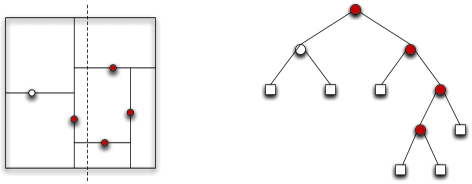
Figure 3: An example of a $2$-d tree is shown: on the left, the partition of $[0,1]^{2}$ induced by the points; on the right, the corresponding binary tree. The colored nodes are the ones that are visited when performing the partial match query materialized by the dashed line.

Partial match queries. From now on, we assume that data consists of a set of independent random points, uniformly distributed on the unit square. Unlike in the case of quadtrees, the direction of a partial match query line with respect to the direction of the root does matter. Let $C_{n}^{=}(t)$ and $C^{\perp}_{n}(t)$ denote the number of nodes visited by a partial match for a query at position $t\in[0,1]$ when the directions of the split at the root and the query are parallel and perpendicular, respectively. Subsequently, we will analyze both quantities synchronously as far as possible. We will always consider directions with respect to the query line, and although some of the expressions (for the sizes of the regions, e.g.) will be symmetric, we keep them distinct for the sake of clarity. (We also assume without loss of generality that the query line is always vertical, and that the direction of the cut at the root may change.)

As in a quadtree, a node is visited by a partial match query if and only if it is inserted in a subregion that intersects the query line. Unfortunately, these nodes are not easily identifiable after the insertion of $n$ points; the value of the quantity $C_{n}^{=}(s)$ is obtained by adding twice the number of lines intersecting the query line at $s$ and the number of boxes that are intersected by the query line and will have their next split perpendicular to the query line (i.e., the depth of the corresponding external nodes in the tree have odd parity).

Recursive decompositions. Let $(U,V)$ be the first point which partitions the unit square. By construction, since the directions of the partitioning lines alternate, both processes $C_{n}^{=}(t)$ and $C_{n}^{\perp}(t)$ are coupled: when the query line is perpendicular to the split direction, the recursive search occurs in both child sub-regions whose sizes we denote by $N_{n}$ and $S_{n}$, and we have

$$C_{n}^{\perp}(s)\stackrel{{\scriptstyle d}}{{=}}1+C^{(=,1)}_{N_{n}}(s)+C^{(=,2)}_{S_{n}}(s);$$ (38)

when the query line and the first split at the root are parallel, only one of the sub-regions (of sizes $L_{n}$ and $R_{n}$) is recursively visited, and we have

$$C_{n}^{\perp}(s)\stackrel{{\scriptstyle d}}{{=}}1+\mathbf{1}_{\{{s<U}\}}C^{(=,1)}_{L_{n}}\biggl{(}\frac{s}{U}\biggr{)}+\mathbf{1}_{\{{s\geq U}\}}C^{(=,2)}_{R_{n}}\biggl{(}\frac{s-U}{1-U}\biggr{)}.$$ (39)

Here $(C^{(=,1)}_{n})_{n\geq 0},(C_{n}^{(=,2)})_{n\geq 0}$ are independent copies of $(C^{=}_{n})_{n\geq 0}$, independent of $(N_{n},S_{n})$ in (38) and $(C^{(\perp,1)}_{n})_{n\geq 0}$, $(C^{(\perp,2)})_{n\geq 0}$ are independent copies of $(C^{\perp}_{n})_{n\geq 0}$, independent of $(L_{n},R_{n})$ in (39). Moreover, here and in the following distributional recurrences and fixed-point equations involving a parameter $s\in[0,1]$ are to be understood on the level of càdlàg or continuous functions unless stated otherwise.

As in the case of partial match in random quadtrees, the expected value at a random uniform query line $\xi$, independent of the tree is of order $n^{\beta}$ for the same constant $\beta$ defined in (1), and we have

$$\mathbf{E}\bigl{[}C_{n}^{=}(\xi)\bigr{]}\sim\kappa_{=}n^{\beta},\qquad\mathbf{E}\bigl{[}C_{n}^{\perp}(\xi)\bigr{]}\sim\kappa_{\perp}n^{\beta}$$

for some constants $\kappa_{=}>0,\kappa_{\perp}>0$. This was first proved by Flajolet and Puech FlPu1986 . A more detailed analysis by Chern and Hwang ChHw2006 shows that

$$\qquad\mathbf{E}\bigl{[}C_{n}^{=}(\xi)\bigr{]} = \kappa_{=}n^{\beta}-2+O\bigl{(}n^{\beta-1}\bigr{)},\qquad\kappa_{=}=\frac{13(3-5\beta)}{4}\cdot\frac{\Gamma(2\beta+2)}{\Gamma(\beta+1)^{3}},$$ (40)

$$\mathbf{E}\bigl{[}C_{n}^{\perp}(\xi)\bigr{]} = \kappa_{\perp}n^{\beta}-3+O\bigl{(}n^{\beta-1}\bigr{)},\qquad\kappa_{\perp}=\frac{13(2\beta-1)}{2}\cdot\frac{\Gamma(2\beta+2)}{\Gamma(\beta+1)^{3}}.$$ (41)

Observe that $\kappa_{=}=\frac{1}{2}13(3-5\beta)\kappa$ and $\kappa_{\perp}=13(2\beta-1)\kappa$, where $\kappa$ is the leading constant for $\mathbf{E}[{C_{n}(\xi)}]$ in the case of quadtrees defined in (1).

Homogeneous recursive relations and limit behavior. For our purposes, and although it yields more complex expressions, it is more convenient to expand the recursion one more level to obtain recursive relations that only involve quantities of the same type, only $(C_{n}^{=})_{n\geq 0}$ or only $(C_{n}^{\perp})_{n\geq 0}$: each one of the first two sub-region at the root is eventually split, and this gives rise to a partition into four regions at level two of the tree. Let $(U_{\ell},V_{\ell})$ and $(U_{r},V_{r})$ be, respectively, the first points on each side (left and right) of the first cut, when it is parallel to the query line. Let also $(U_{u},V_{u})$ and $(U_{d},V_{d})$ be the first points on each side of the cut (up and down) when it is perpendicular to the query line. Note that $U,V_{\ell},V_{r}$ are independent and uniform on $[0,1]$, and so are $V,U_{u}$ and $U_{d}$.

Let $I_{=,1}^{(n)},\ldots,I_{=,4}^{(n)}$ and $I_{\perp,1}^{(n)},\ldots,I_{\perp,4}^{(n)}$ denote the number of data points falling in these regions when the root and the query line are parallel and perpendicular, respectively. The distributions of $I_{=,1}^{(n)},\ldots,I_{=,4}^{(n)}$ on the one hand, and $I_{\perp,1}^{(n)},\ldots,I_{\perp,4}^{(n)}$ on the other hand are slightly more involved than in the case of quadtrees. One has, for example, given the values of $U,V_{\ell},V_{r}$ it holds

$$I_{=,1}^{(n)}\stackrel{{\scriptstyle d}}{{=}}\operatorname{Bin}\bigl{(}\bigl{(}\operatorname{Bin}(n-1;U)-1\bigr{)}_{+},V_{\ell}\bigr{)}$$

and given $V,U_{d},U_{u}$

$$I_{\perp,1}^{(n)}\stackrel{{\scriptstyle d}}{{=}}\operatorname{Bin}\bigl{(}\bigl{(}\operatorname{Bin}(n-1;V)-1\bigr{)}_{+},U_{d}\bigr{)},$$

where the inner and outer binomials are independent. Analogous expressions hold true for the remaining quantities.

Substituting (38) and (39) into each other gives

$$C_{n}^{=}(s) \stackrel{{\scriptstyle d}}{{=}} 1+\mathbf{1}_{\{{s<U}\}}\biggl{[}\mathbf{1}_{\{{L_{n}>0}\}}+C^{(=,1)}_{I_{=,1}^{(n)}}\biggl{(}\frac{s}{U}\biggr{)}+C^{(=,2)}_{I_{=,2}^{(n)}}\biggl{(}\frac{s}{U}\biggr{)}\biggr{]}$$

$${}+\mathbf{1}_{\{{s\geq U}\}}\biggl{[}\mathbf{1}_{\{{R_{n}>0}\}}+C^{(=,3)}_{I_{=,3}^{(n)}}\biggl{(}\frac{s-U}{1-U}\biggr{)}+C^{(=,4)}_{I_{=,4}^{(n)}}\biggl{(}\frac{s-U}{1-U}\biggr{)}\biggr{]}$$

and

$$C_{n}^{\perp}(s) \stackrel{{\scriptstyle d}}{{=}} 1+\mathbf{1}_{\{{S_{n}>0}\}}+\mathbf{1}_{\{{N_{n}>0}\}}+\mathbf{1}_{\{{s<U_{d}}\}}C^{(\perp,1)}_{I_{\perp,1}^{(n)}}\biggl{(}\frac{s}{U_{d}}\biggr{)}$$

$${}+\mathbf{1}_{\{{s<U_{u}}\}}C^{(\perp,2)}_{I_{\perp,2}^{(n)}}\biggl{(}\frac{s}{U_{u}}\biggr{)}$$

$${}+\mathbf{1}_{\{{s\geq U_{d}}\}}C^{(\perp,3)}_{I_{\perp,3}^{(n)}}\biggl{(}\frac{s-U_{d}}{1-U_{d}}\biggr{)}+\mathbf{1}_{\{{s\geq U_{u}}\}}C^{(\perp,4)}_{I_{\perp,4}^{(n)}}\biggl{(}\frac{s-U_{u}}{1-U_{u}}\biggr{)},$$

where $(C^{(=,i)}_{n})_{n\geq 0}$, $i=1,\ldots,4$, are independent copies of $(C^{=}_{n})_{n\geq 0}$, which are also independent of the family $(U,I_{=,1}^{(n)},I_{=,2}^{(n)},I_{=,3}^{(n)},I_{=,4}^{(n)})$ in (7.1), and $(C^{(\perp,i)}_{n})_{n\geq 0}$, $i=1,\ldots,4$, are independent copies of $(C^{\perp}_{n})_{n\geq 0}$, which are also independent of $(U_{d},U_{u},I_{\perp,1}^{(n)},I_{\perp,2}^{(n)},I_{\perp,3}^{(n)},I_{\perp,4}^{(n)})$ in (7.1). Asymptotically, any limit $Z^{=}(s)$ of $n^{-\beta}C_{n}^{=}(s)$ should satisfy the following fixed-point equation:

$$Z^{=}(s) \stackrel{{\scriptstyle d}}{{=}} \mathbf{1}_{\{{s<U}\}}\biggl{[}(UV_{\ell})^{\beta}Z^{(=,1)}\biggl{(}\frac{s}{U}\biggr{)}+\bigl{(}U(1-V_{\ell})\bigr{)}^{\beta}Z^{(=,2)}\biggl{(}\frac{s}{U}\biggr{)}\biggr{]}$$

$${}+\mathbf{1}_{\{{s\geq U}\}}\biggl{[}\bigl{(}(1-U)V_{r}\bigr{)}^{\beta}Z^{(=,3)}\biggl{(}\frac{s-U}{1-U}\biggr{)}$$

$$\hskip 48.0pt{}+\bigl{(}(1-U)(1-V_{r})\bigr{)}^{\beta}Z^{(=,4)}\biggl{(}\frac{s-U}{1-U}\biggr{)}\biggr{]},$$

where $Z^{(=,i)}$, $i=1,\ldots,4$, are independent copies of $Z^{=}$, independent of $(U,V_{\ell},V_{r})$. Likewise any limit of $n^{-\beta}C_{n}^{\perp}(s)$ should satisfy

$$Z^{\perp}(s) \stackrel{{\scriptstyle d}}{{=}} \mathbf{1}_{\{{s<U_{d}}\}}(U_{d}V)^{\beta}Z^{(\perp,1)}\biggl{(}\frac{s}{U_{d}}\biggr{)}+\mathbf{1}_{\{{s<U_{u}}\}}\bigl{(}U_{u}(1-V)\bigr{)}^{\beta}Z^{(\perp,2)}\biggl{(}\frac{s}{U_{u}}\biggr{)}$$

$${}+\mathbf{1}_{\{{s\geq U_{d}}\}}\bigl{(}(1-U_{d})V\bigr{)}^{\beta}Z^{(\perp,3)}\biggl{(}\frac{s-U_{d}}{1-U_{d}}\biggr{)}$$

$${}+\mathbf{1}_{\{{s\geq U_{u}}\}}\bigl{(}(1-U_{u})(1-V)\bigr{)}^{\beta}Z^{(\perp,4)}\biggl{(}\frac{s-U_{u}}{1-U_{u}}\biggr{)},$$

where $Z^{(\perp,i)}$, $i=1,\ldots,4$, are independent copies of $Z^{\perp}$, independent of $(U_{d},U_{u},V).$ Moreover, according to (38) and (39), we expect a connection between these two limits. This will be stated in the first result of the next section and always allows us to focus on $C_{n}^{=}(s)$ first. The result for $C_{n}^{\perp}$ can then be deduced easily afterwards.

7.2 About the conditions to use the contraction argument

Existence of continuous limit processes. As in the case of quadtrees, one of the first steps consists of showing the existence of the limit processes $Z^{\perp}$ and $Z^{=}$.

Proposition 18.

There exist two random continuous processes $Z^{=},Z^{\perp}$ with $\mathbf{E}[{Z^{=}(s)}]=\mathbf{E}[{Z^{H}(s)}]=h(s)$, finite absolute moments of all orders such that $Z^{=}$ satisfies (7.1) and $Z^{\perp}$ satisfies (7.1). The laws of $Z^{=}$ and $Z^{\perp}$ are both unique under these constraints. Additionally:

• $$\frac{2}{\beta+1}Z^{\perp}(s)\stackrel{{\scriptstyle d}}{{=}}V^{\beta}Z^{(=,1)}(s)+(1-V)^{\beta}Z^{(=,2)}(s)$$ (46)

  and

  $$\frac{\beta+1}{2}Z^{=}(s)\stackrel{{\scriptstyle d}}{{=}}\mathbf{1}_{\{{s<U}\}}U^{\beta}Z^{(\perp,1)}\biggl{(}\frac{s}{U}\biggr{)}+\mathbf{1}_{\{{s\geq U}\}}(1-U)^{\beta}Z^{(\perp,2)}\biggl{(}\frac{s-U}{1-U}\biggr{)}.$$

• For every fixed $s\in[0,1]$, $Z^{=}(s)$ is distributed like $Z(s)$ where $Z$ is the process constructed in Section 4. In particular, $\operatorname{Var}({Z^{=}(s)})$ is given in (8) and $\operatorname{Var}({Z^{\perp}(s)})=K_{2}^{\perp}h^{2}(s)$, where

  $$K_{2}^{\perp}=\biggl{(}\frac{2c_{2}}{2\beta+1}\biggl{(}\frac{\beta+1}{2}\biggr{)}^{2}+2\mathrm{B}(\beta+1,\beta+1)\biggl{(}\frac{\beta+1}{2}\biggr{)}^{2}-1\biggr{)},$$ (47)

  and $c_{2}$ is defined in (35).

• If $\xi$ is uniform on $[0,1]$ and independent of $Z^{=},Z^{\perp}$, then $\operatorname{Var}({Z^{=}(\xi)})=\operatorname{Var}({Z(\xi)})$ and

  $$\operatorname{Var}\bigl{(}Z^{\perp}(\xi)\bigr{)}$$

  $$\qquad=K_{3}^{\perp}=\biggl{(}\frac{2c_{2}}{2\beta+1}+2\mathrm{B}(\beta+1,\beta+1)\biggr{)}\biggl{(}\frac{\beta+1}{2}\biggr{)}^{2}\mathrm{B}(\beta+1,\beta+1)$$ (48)

  $$\hskip 30.0pt\qquad\quad{}-\biggl{(}\mathrm{B}\biggl{(}\frac{\beta}{2}+1,\frac{\beta}{2}+1\biggr{)}\biggr{)}^{2}.$$

The fixed-point equation (7.1) is very similar to that in (3.1), and we use the approach that has proved fruitful in Section 4. More precisely, the construction of $Z(s)$ slightly modified to $Z^{=}(s)$. Define the operator $G^{=}:[0,1]^{3}\times\mathcal{C}[0,1]^{4}\to\mathcal{C}[0,1]$ by

$$G^{=}(x,y,z,f_{1},f_{2},f_{3},f_{4})(s)$$

$$\qquad=\mathbf{1}_{\{{s<x}\}}\biggl{[}(xy)^{\beta}f_{1}\biggl{(}\frac{s}{x}\biggr{)}+\bigl{(}x(1-y)\bigr{)}^{\beta}f_{2}\biggl{(}\frac{s}{x}\biggr{)}\biggr{]}$$

$$\qquad\quad{}+\mathbf{1}_{\{{s\geq x}\}}\biggl{[}\bigl{(}(1-x)z\bigr{)}^{\beta}f_{3}\biggl{(}\frac{s-x}{1-x}\biggr{)}+\bigl{(}(1-x)(1-z)\bigr{)}^{\beta}f_{4}\biggl{(}\frac{s-x}{1-x}\biggr{)}\biggr{]}.$$

Then let (as in Section 4)

$$Z_{n+1}^{=,u}=G^{=}\bigl{(}U_{u},V_{u},W_{u},Z_{n}^{=,u1},Z_{n}^{=,u2},Z_{n}^{=,u3},Z_{n}^{=,u4}\bigr{)},\qquad Z_{0}^{=,u}=h(s)$$

for all $u\in\mathcal{T}$, where $\{U_{v},v\in\mathcal{T}\},\{V_{v},v\in\mathcal{T}\}$ and $\{W_{v},v\in\mathcal{T}\}$ are three independent families of i.i.d. $[0,1]$-uniform random variables. Lemma 10 remains true for $Z_{n}^{=}:=Z_{n}^{=,\varnothing}$ since $W_{n}^{=}$ equals $W_{n}$ in distribution where $W_{n}$ appears in (4). Since also $L_{n}^{=}$ and $L_{n}$ (appearing in Lemma 24) coincide in distribution, (27) holds true for $Z_{n}^{=}$ and therefore Proposition 9 remains valid. The existence of all moments of $\sup_{s\in[0,1]}Z^{=}(s)$ follows in the same way. Finally, note that $Z^{=}_{n}(s)$ is distributed as $Z_{n}(s)$ for all fixed $n,s$, hence the one-dimensional distributions of $Z^{=}$ and $Z$ coincide. It is now easy to see that $Z^{\perp}$ defined by (46) solves (7.1). The uniqueness of $Z^{=}(s)$ [resp., $Z^{=}(s)$] follows by contraction with respect to the $\zeta_{2}$ metric; compare Lemma 18 in NeSu2011a . Finally, the variance of $Z^{\perp}(s)$ can be computed as in Section 6 but it is much easier to use (46), we omit the calculations.

Uniform convergence of the mean. Comparing construction and recurrence for partial match queries in $2$-d trees and quadtrees it seems very likely that this quantities are not only of the same asymptotic order in the case of a uniform query but also closely related for fixed $s\in[0,1]$ and $n\in\mathbb{N}$. This can be formalized by the following lemma:

Lemma 19.

For any $s\in[0,1]$ and $n\in\mathbb{N}$, we have

$$\tfrac{1}{5}\mathbf{E}\bigl{[}C_{n}(s)\bigr{]}\leq\mathbf{E}\bigl{[}C_{n}^{=}(s)\bigr{]}\leq 2\mathbf{E}\bigl{[}C_{n}(s)\bigr{]}.$$

We prove both bounds by induction on $n$ using the recursive decompositions (3.1), (7.1). Both inequalities are obviously true for $n=0,1$. Assume that the assertions were true for all $m\leq n-1$ and $s\in[0,1]$. We start with the upper bound which is easier. By (7.1), we have

$$\mathbf{E}\bigl{[}C_{n}^{=}(s)\bigr{]} \leq 2+\mathbf{E}\biggl{[}\mathbf{1}_{\{{s<U}\}}\biggl{[}C^{(=,1)}_{I_{=,1}^{(n)}}\biggl{(}\frac{s}{U}\biggr{)}+C^{(=,2)}_{I_{=,2}^{(n)}}\biggl{(}\frac{s}{U}\biggr{)}\biggr{]}\biggr{]}$$

$${}+\mathbf{E}\biggl{[}\mathbf{1}_{\{{s\geq U}\}}\biggl{[}C^{(=,3)}_{I_{=,3}^{(n)}}\biggl{(}\frac{s-U}{1-U}\biggr{)}+C^{(=,4)}_{I_{=,4}^{(n)}}\biggl{(}\frac{s-U}{1-U}\biggr{)}\biggr{]}\biggr{]}.$$

Hence, it suffices to show that

$$\mathbf{E}\biggl{[}\mathbf{1}_{\{{s<U}\}}C^{(=,1)}_{I_{=,1}^{(n)}}\biggl{(}\frac{s}{U}\biggr{)}\biggr{]}\leq 2\mathbf{E}\biggl{[}\mathbf{1}_{\{{s<U}\}}C^{(1)}_{I_{1}^{(n)}}\biggl{(}\frac{s}{U}\biggr{)}\biggr{]}.$$

This can be done in two steps. First, by conditioning on $I_{=,1}^{(n)}$ and $U$, using the induction hypothesis, we have

$$\mathbf{E}\biggl{[}\mathbf{1}_{\{{s<U}\}}C^{(=,1)}_{I^{(n)}_{=,1}}\biggl{(}\frac{s}{U}\biggr{)}\biggr{]}\leq 2\mathbf{E}\biggl{[}\mathbf{1}_{\{{s<U}\}}C^{(1)}_{I^{(n)}_{=,1}}\biggl{(}\frac{s}{U}\biggr{)}\biggr{]}.$$

Finally, conditioning on $U$, $I^{(n)}_{=,1}$ is stochastically smaller than $I^{(n)}_{1}$ which gives

$$\mathbf{E}\biggl{[}\mathbf{1}_{\{{s<U}\}}C^{(1)}_{I^{(n)}_{=,1}}\biggl{(}\frac{s}{U}\biggr{)}\biggr{]}\leq 2\mathbf{E}\biggl{[}\mathbf{1}_{\{{s<U}\}}C^{(1)}_{I_{1}^{(n)}}\biggl{(}\frac{s}{U}\biggr{)}\biggr{]}$$

by monotonicity of $n\to\mathbf{E}[{C_{n}(s)}]$. For the lower bound, note that

$$\mathbf{E}\bigl{[}C_{n}^{=}(s)\bigr{]} \geq 1+\mathbf{E}\biggl{[}\mathbf{1}_{\{{s<U}\}}\biggl{[}C^{(=,1)}_{I_{=,1}^{(n)}}\biggl{(}\frac{s}{U}\biggr{)}+C^{(=,2)}_{I_{=,2}^{(n)}}\biggl{(}\frac{s}{U}\biggr{)}\biggr{]}\biggr{]}$$

$${}+\mathbf{E}\biggl{[}\mathbf{1}_{\{{s\geq U}\}}\biggl{[}C^{(=,3)}_{I_{=,3}^{(n)}}\biggl{(}\frac{s-U}{1-U}\biggr{)}+C^{(=,4)}_{I_{=,4}^{(n)}}\biggl{(}\frac{s-U}{1-U}\biggr{)}\biggr{]}\biggr{]}.$$

Therefore, it is enough to prove

$$\mathbf{E}\biggl{[}\mathbf{1}_{\{{s<U}\}}C^{(=,1)}_{I_{=,1}^{(n)}}\biggl{(}\frac{s}{U}\biggr{)}\biggr{]}\geq\frac{1}{5}\biggl{(}\mathbf{E}\biggl{[}\mathbf{1}_{\{{s<U}\}}C^{(1)}_{I_{1}^{(n)}}\biggl{(}\frac{s}{U}\biggr{)}\biggr{]}-1\biggr{)}.$$

This can be done as for the upper bound. First, by the induction hypothesis, we have

$$\mathbf{E}\biggl{[}\mathbf{1}_{\{{s<U}\}}C^{(=,1)}_{I^{(n)}_{=,1}}\biggl{(}\frac{s}{U}\biggr{)}\biggr{]}\geq\frac{1}{5}\mathbf{E}\biggl{[}\mathbf{1}_{\{{s<U}\}}C^{(1)}_{I^{(n)}_{=,1}}\biggl{(}\frac{s}{U}\biggr{)}\biggr{]}.$$

The result follows as for the upper bound by the fact that $I_{=,1}^{(n)}$ is stochastically larger than $(I_{1}^{(n)}-1)^{+}$ and $C^{(1)}_{(I_{1}^{(n)}-1)^{+}}\geq C^{(1)}_{I_{1}^{(n)}}-1$. Recalling (40) and (41), it is natural to introduce the constants

$$K_{1}^{=}=\frac{\kappa_{=}}{\mathrm{B}({\beta}/{2}+1,{\beta}/{2}+1)},\qquad K_{1}^{\perp}=\frac{\kappa_{\perp}}{\mathrm{B}({\beta}/{2}+1,{\beta}/{2}+1)}$$

(49)

$$\eqntext{\mbox{with }\displaystyle K_{1}^{\perp}=\frac{2}{1+\beta}K_{1}^{=},}$$ (50)

and the functions $\mu_{1}^{\perp}(s)=K_{1}^{\perp}h(s)$, and $\mu_{1}^{=}(s)=K_{1}^{=}h(s).$

Proposition 20.

There exists $\varepsilon_{=}>0$ such that

$$\sup_{s\in[0,1]}\bigl{|}n^{-\beta}\mathbf{E}\bigl{[}C_{n}^{=}(s)\bigr{]}-\mu_{1}^{=}(s)\bigr{|}=O\bigl{(}n^{-\varepsilon_{=}}\bigr{)},$$

and the analogous result holds true for $\mathbf{E}[{C_{n}^{\perp}(s)}]$.

We proceed as in Section 5 by considering the continuous-time process $P_{t}^{=}(s)$. Since we have already proved an analogous result for the case of quadtree, we give a brief sketch that focuses on the few locations where the arguments have to be modified.

Sketch of proof The first step is to prove point-wise convergence which is done as Curien and Joseph CuJo2010 . By Lemma 19, using a Poisson$(t)$ number of points, we have

$$\tfrac 15\mathbf{E}\bigl{[}P_{t}(s)\bigr{]}\leq\mathbf{E}\bigl{[}P^{=}_{t}(s)\bigr{]}\leq 2\mathbf{E}\bigl{[}P_{t}(s)\bigr{]}.$$ (51)

Let $\tau_{1}^{=}$ be the arrival time of the first point which yields a partitioning line that intersects the query line $\{x=s\}$, and let $Q_{1}^{=}=Q_{1}^{=}(s)$ be the lower of the two rectangles created by this cut (for the expected value we are about to compute, they both look the same). Let $\xi_{1}^{=}:=\xi_{1}^{=}(s)$ be the relative position of the query line $s$ within the rectangle $Q_{1}^{=}$ and $M_{1}^{=}=\operatorname{Leb}(Q_{1}^{=})$. Then, denoting $\tau$ the arrival time of the first point in the process, we have

$$\mathbf{E}\bigl{[}P_{t}^{=}(s)\bigr{]}=\mathbf{P}(t\geq\tau)+\mathbf{P}\bigl{(}t\geq\tau_{1}^{=}\bigr{)}+2\mathbf{E}\bigl{[}\tilde{P}^{=}_{M_{1}^{=}t-\tau_{1}^{=}}\bigl{(}\xi_{1}^{=}\bigr{)}\bigr{]},$$

where $(\tilde{P}^{=}(t))_{t\geq 0}$ denotes an independent copy of $(P^{=}(t))_{t\geq 0}$ and $\tilde{P}^{=}(t)=0$ for $t<0$. Similarly, let $\tau_{k}^{=}$ be the arrival time of the first point which cuts $Q_{k-1}^{=}$ perpendicularly to the query line. Let $Q^{=}_{k}$ be the lower of the two rectangles created by this cut, and let $\xi_{k}^{=}$ be the position of the query line $s$ relative to the rectangle $Q_{k}^{=}$. With this notation and $M_{k}^{=}=\operatorname{Leb}(Q_{k}^{=})$, we have

$$\mathbf{E}\bigl{[}P_{t}^{=}(s)\bigr{]}=g_{k}^{=}(t)+2^{k}\mathbf{E}\bigl{[}\tilde{P}^{=}_{M_{k}^{=}t-\tau_{k}^{=}}\bigl{(}\xi_{k}^{=}\bigr{)}\bigr{]},$$

where $0\leq g_{k}^{=}(t)\leq 2^{k+1}$.

We need to modify the inter-arrival times ${\zeta^{\prime}}_{k}^{=}=\tau_{k}^{=}-\tau_{k-1}^{=}$. We can split ${\zeta^{\prime}}_{k}^{=}$ in the time it takes for the first vertical point to fall in $Q_{k-1}^{=}$ which we denote by ${\zeta^{\prime}}_{k}^{=,1}$ and the remaining time by ${\zeta^{\prime}}_{k}^{=,2}$. Letting $M_{k}^{=}=\operatorname{Leb}(Q_{k}^{=})$, the normalized versions of the inter-arrival times with unit mean are

$$\zeta_{k}^{=,1} = {\zeta^{\prime}}_{k}^{=,1}\cdot M_{k-1}^{=},$$

$$\zeta_{k}^{=,2} = \biggl{(}\frac{\xi^{=}_{k}}{\xi^{=}_{k-1}}\mathbf{1}_{\{{\xi^{=}_{k}<\xi^{=}_{k-1}}\}}+\frac{\xi^{=}_{k-1}}{\xi^{=}_{k}}\mathbf{1}_{\{{\xi^{=}_{k}\geq\xi^{=}_{k-1}}\}}\biggr{)}{\zeta^{\prime}}_{k}^{=,2}\cdot M_{k-1}^{=}\geq{\zeta^{\prime}}_{k}^{=,2}\cdot M_{k-1}^{=}.$$

Write $\mathcal{M}_{k}=M_{k}/M_{k-1}$. Observe that, given $\mathcal{M}_{0}^{=},\ldots,\mathcal{M}_{k}^{=}$, the random variable $F_{k}^{=}=M_{k}^{=}\cdot\tau_{k}^{=}$ is not independent of $(\xi_{\ell})_{0\leq\ell\leq k}$, a property which is used in CuJo2010 and in the proof of Lemma 15 in the present paper. However we can use the trivial lower bound $0\leq F_{k}$ and the upper bound obtained by bounding ${\zeta^{\prime}}_{k}^{=,2}$ from above by $\zeta_{k}^{=,2}/M_{k-1}^{=}$. Then, using almost sure monotonicity of $P_{t}(s)$ (in $t$) and (51) to transform bounds for the mean in the quadtree to bounds in the $2$-d tree (and vice versa), it is easy to see that the techniques of Section 4 in CuJo2010 work equally well in this case. The limit $\mu_{1}^{=}(s)$ is identified as in Section 5 of CuJo2010 since both limits satisfy the same fixed-point equation.

The generalization to uniform convergence with polynomial rate can be worked out as in Section 5 (of the present document) using the modifications we have described above. The constants appearing in the course of Section 5 need to be modified, but $\varepsilon_{=}$ may be chosen to equal the value of $\varepsilon$ in Proposition 13. The de-Poissonization is routine, and we omit the details.

Finally, we indicate how to proceed with $\mathbf{E}[{C_{n}^{\perp}(s)}]$. The arguments above can be used to treat prove uniform convergence of $n^{-\beta}\mathbf{E}[{C_{n}^{\perp}(s)}]$ on $[0,1]$; we present a direct approach relying on (38). We have

$$n^{-\beta}\mathbf{E}\bigl{[}C_{n}^{\perp}(s)\bigr{]} = n^{-\beta}+2n^{-\beta}\mathbf{E}\bigl{[}C^{=}_{S_{n}}(s)\bigr{]}$$

$$= n^{-\beta}+2\int_{0}^{1}\sum_{k=0}^{n-1}\bigl{(}\mu_{1}^{=}(s)+O\bigl{(}k^{-\varepsilon_{=}}\bigr{)}\bigr{)}\frac{k^{\beta}}{n^{\beta}}\mathbf{P}\bigl{(}\operatorname{Bin}(n-1,v)=k\bigr{)}\,dv$$

$$= n^{-\beta}+2\mu_{1}^{=}(s)\cdot\frac{\mathbf{E}[{\operatorname{Bin}(n-1,V)^{\beta}}]}{n^{\beta}}$$

$${}+O\bigl{(}n^{-\beta}\mathbf{E}\bigl{[}\operatorname{Bin}(n-1,V)^{\beta-\varepsilon_{=}}\bigr{]}\bigr{)}$$

$$= \mu_{1}^{\perp}(s)+O\bigl{(}n^{-\varepsilon_{=}}\bigr{)},$$

uniformly in $s\in[0,1]$ using Minkowski’s inequality, the concentration for binomial in (21), and (7.2) for the first term and Jensen’s inequality for the second.

7.3 The limiting behavior in $2$-d trees

We are finally ready to state the version of our main result for $2$-d trees. It is proved along the same lines we used for the case of quadtrees, and we omit the details.

Theorem 21

With the processes $Z^{=}$ and $Z^{\perp}$ of Proposition 18 we have

$$\biggl{(}\frac{C_{n}^{=}(s)}{K_{1}^{=}n^{\beta}}\biggr{)}_{s\in[0,1]}\rightarrow\bigl{(}Z^{=}(s)\bigr{)}_{s\in[0,1]},\qquad\biggl{(}\frac{C_{n}^{\perp}(s)}{K_{1}^{\perp}n^{\beta}}\biggr{)}_{s\in[0,1]}\rightarrow\bigl{(}Z^{\perp}(s)\bigr{)}_{s\in[0,1]},$$

in distribution in $\mathcal{D}[0,1]$ endowed with the Skorokhod topology. Here $K_{1}^{=}$ and $K_{1}^{\perp}$ are defined in (7.2). For $s\in[0,1]$

$$n^{-\beta}\mathbf{E}\bigl{[}C_{n}^{=}(s)\bigr{]}\rightarrow K_{1}^{=}h(s),\qquad n^{-2\beta}\operatorname{Var}\bigl{(}C^{=}_{n}(s)\bigr{)}\rightarrow\bigl{(}K_{1}^{=}\bigr{)}^{2}K_{2}h(s)^{2}$$

and

$$n^{-\beta}\mathbf{E}\bigl{[}C_{n}^{\perp}(s)\bigr{]}\rightarrow K_{1}^{\perp}h(s),\qquad n^{-2\beta}\operatorname{Var}\bigl{(}C^{\perp}_{n}(s)\bigr{)}\rightarrow\bigl{(}K_{1}^{\perp}\bigr{)}^{2}K_{2}^{\perp}h(s)^{2},$$

where $K_{2}$ is given in (8) and $K_{2}^{\perp}$ in (47).

If $\xi$ is uniformly distributed on $[0,1]$, independent of $(C_{n}^{=})_{n\geq 0},(C_{n}^{\perp})_{n\geq 0}$ and $Z^{=},Z^{\perp}$, then

$$\frac{C^{=}_{n}(\xi)}{K_{1}^{=}n^{\beta}}\stackrel{{\scriptstyle d}}{{\longrightarrow}}Z^{=}(\xi),\qquad\frac{C^{\perp}_{n}(\xi)}{K_{1}^{\perp}n^{\beta}}\stackrel{{\scriptstyle d}}{{\longrightarrow}}Z^{\perp}(\xi),$$

with convergence of the first two moments in both cases. In particular

$$\operatorname{Var}\bigl{(}C^{=}_{n}(\xi)\bigr{)}\sim K_{4}^{=}n^{2\beta},\qquad\operatorname{Var}\bigl{(}C^{\perp}_{n}(\xi)\bigr{)}\sim K_{4}^{\perp}n^{2\beta},$$

where $K_{4}^{=}=(K_{1}^{=})^{2}K_{3}\approx 0.69848$, $K_{4}^{\perp}=(K_{1}^{\perp})^{2}K^{V}_{3}\approx 0.77754,$ with $K_{3}=\operatorname{Var}({Z(\xi)})$ in (3) and $K_{3}^{\perp}$ in (• ‣ 18).

Note that since $Z^{=}(s)$ equals $Z(s)$ in distribution for fixed $s\in[0,1]$ we can characterize $Z^{=}(s)$ as in (9). (46) together with Proposition 18 implies that for fixed $s\in[0,1]$

$$Z^{\perp}(s)\stackrel{{\scriptstyle d}}{{=}}\Psi^{\perp}\cdot h(s)\qquad\mbox{with }\Psi^{\perp}=\frac{\beta+1}{2}\bigl{(}V^{\beta}\Psi+(1-V)^{\beta}\Psi^{\prime}\bigr{)},$$

where $\Psi^{\prime}$ is an independent copy of $\Psi$, $\Psi$ being defined in Theorem 5 and $V$ is independent of $(\Psi,\Psi^{\prime})$. In particular, we have

$$\mathbf{E}\bigl{[}\bigl{(}\Psi^{\perp}\bigr{)}^{m}\bigr{]}=\biggl{(}\frac{\beta+1}{2}\biggr{)}^{m}\sum_{\ell=0}^{m}\pmatrix{m\cr\ell}\mathrm{B}\bigl{(}\beta\ell+1,\beta(m-\ell)+1\bigr{)}c_{\ell}c_{m-\ell}$$

for $m\geq 2$ where $c_{m}=\mathbf{E}[{\Psi^{m}}]$ satisfies recursion (6) and $c_{0}=c_{1}=1$.

Also, as in the quadtree case, it is possible to give convergence of mixed moments of arbitrary order, compare Corollary 6, and distributional and moment convergence of the suprema of the processes after rescaling as in Theorem 4.

Appendix A About the geometry of random quadtrees

Lemma 22.

Let $W_{n}$ denote the maximum width of a cell at level $n$ in the construction of $Z_{n}$ and $c<1$. Then

$$\mathbf{P}\bigl{(}W_{n}\geq c^{n}\bigr{)}\leq\bigl{(}4e\log(1/c)\bigr{)}^{n}.$$

Let $U_{i}$, $i\geq 1$ be a family of i.i.d. $[0,1]$-uniform random variables and $E_{i}$, $i\geq 1$, be a family of i.i.d. $\operatorname{exponential}(1)$ random variables. Then, the union bound and a large deviations argument yields

$$\mathbf{P}\bigl{(}W_{n}\geq c^{n}\bigr{)} \leq 4^{n}\cdot\mathbf{P}\bigl{(}U_{1}\cdot U_{2}\cdots U_{n}\geq c^{n}\bigr{)}$$

$$= 4^{n}\cdot\mathbf{P}\Biggl{(}\sum_{i=1}^{n}E_{i}\leq n\log(1/c)\Biggr{)}$$

$$\leq 4^{n}\exp\bigl{(}-n\bigl{(}\log(1/c)-1-\log\log(1/c)\bigr{)}\bigr{)}$$

$$\leq \bigl{(}4e\log(1/c)\bigr{)}^{n}$$

as desired.

Lemma 23.

Let $F_{k}$ be the fill-up level of a random quadtree of size $k$. Then, for every integer number $x>22$ there exists an integer $n_{0}(x)$ with

$$\mathbf{P}(F_{x^{n}}<n)\leq 4^{n+1}x^{-n/100},\qquad n\geq n_{0}(x).$$

We consider the $4^{n}$ possible nodes in level $n$. By symmetry each of them is occupied by a key with the same probability. Looking at a specific one, for example, the leftmost, size of the corresponding subtree is stochastically bounded by $\operatorname{Bin}(x^{n};U_{1}V_{1}\cdots U_{n}V_{n})-n$ where $\{U_{i},i\geq 1\}$ and $\{V_{i},i\geq 1\}$ are independent families of i.i.d. $[0,1]$-uniform random variables. Then by the union bound applied to the $4^{n}$ cells at level $n$, using Chernoff’s inequality, we have

$$\mathbf{P}(F_{x^{n}}<n) \leq 4^{n}\cdot\mathbf{P}\bigl{(}\operatorname{Bin}\bigl{(}x^{n};U_{1}V_{1}\cdots U_{n}V_{n}\bigr{)}\leq n\bigr{)}$$

$$\leq 4^{n}\cdot\exp\bigl{(}-\bigl{(}1-n2^{-n}\bigr{)}^{2}2^{n+1}\bigr{)}$$

$${}+4^{n}\mathbf{P}\biggl{(}U_{1}V_{1}\cdots U_{n}V_{n}\leq\biggl{(}\frac{2}{x}\biggr{)}^{n}\biggr{)}.$$

However, using once again the large deviations principle for sums of i.i.d. exponential random variables $E_{i},i\geq 1$,

$$\mathbf{P}\bigl{(}U_{1}V_{1}\ldots U_{n}V_{n}\leq(2/x)^{n}\bigr{)} = \mathbf{P}\Biggl{(}\sum_{i=1}^{2n}E_{i}\geq n\log(x/2)\Biggr{)}$$

$$\leq \exp\biggl{(}-2n\biggl{(}\frac{\log(x/2)}{2}-1-\log\frac{\log(x/2)}{2}\biggr{)}\biggr{)}$$

$$\leq x^{-n/100}$$

for all $x>22$ since then $\frac{e^{2}}{2}\log^{2}(x/2)\leq x^{99/100}$. Putting (A) and (A), we obtain

$$\mathbf{P}(F_{x^{n}}<n)\leq 4^{n}\exp\bigl{(}-2^{n-1}\bigr{)}+4^{n}\cdot x^{-n/100}\leq 4^{n+1}x^{-n/100}$$

for $x>22$ and $n$ large enough.

Lemma 24.

There exists $0<\gamma_{0}<1$ such that any positive real number $\gamma<\gamma_{0}$, there exists an integer $n_{1}(\gamma)$ with

$$\mathbf{P}\bigl{(}L_{n}<\gamma^{n}\bigr{)}\leq 6^{n+1}\gamma^{n/201},\qquad n\geq n_{1}(\gamma).$$

The joint distribution of the $x$-coordinates of the vertical lines in the tree developed up to level $n$ is complex. In particular, it is not that of independent uniform points on $[0,1]$. However, we can use a simple coupling with a family of i.i.d. random points on $[0,1]^{2}$ that yields a good enough lower bound on $L_{n}$.

Let $\xi_{i}=(U_{i},V_{i})$, $i\geq 1$ be i.i.d. uniform random points on $[0,1]^{2}$. Let $T_{k}$ be the quadtree obtained by inserting the random points $\xi_{i}$, $1\leq i\leq k$, in this order. Write $D_{i}$ for the depth at which the point $\xi_{i}$ is inserted; so, for instance, $D_{1}=0$. Let $K_{n}$ be the first $k$ for which the tree $T_{k}$ is complete up to level $n$; we mean here that $T_{k}$ should have $4^{n}$ cells at level $n$, so it should have $4^{n-1}$ nodes at level $n-1$. Then, by definition $\{\xi_{i}\dvtx i\geq 1,D_{i}<n\}$ has the distribution of the set of points used to construct the process $Z_{n}$. Obviously, $\{\xi_{i}\dvtx i\geq 1,D_{i}<n\}\subseteq\{\xi_{i}\dvtx 1\leq i\leq K_{n}\},$ and for any natural number $x>0$,

$$\mathbf{P}\bigl{(}L_{n}<\gamma^{n}\bigr{)} \leq \mathbf{P}\bigl{(}\exists i,j\leq K_{n}\dvtx i\neq j,|U_{i}-U_{j}|<\gamma^{n}\bigr{)}$$

$$\leq \mathbf{P}\bigl{(}\exists i,j\leq x^{n}\dvtx i\neq j,|U_{i}-U_{j}|<\gamma^{n}\bigr{)}+\mathbf{P}\bigl{(}K_{n}>x^{n}\bigr{)}$$

$$\leq x^{2n}\cdot 2\gamma^{n}+\mathbf{P}\bigl{(}K_{n}>x^{n}\bigr{)},$$

by the union bound. The random variable $K_{n}$ is related to the fill-up level of a random quadtree, which has been studied by Devroye1987 ; see also DeLa1990 . We could not find a reference giving a precise tail bound, so we proved one here in Lemma 23. We obtain

$$\mathbf{P}\bigl{(}K_{n}>x^{n}\bigr{)}=\mathbf{P}(F_{x^{n}}<n)\leq 4\bigl{(}4x^{-1/100}\bigr{)}^{n}$$

as long as $x\geq 22$ and $n\geq n_{0}(x)$ (the condition for the bound in Lemma 23 to hold). It follows readily that

$$\mathbf{P}\bigl{(}L_{n}<\gamma^{n}\bigr{)} \leq 2\bigl{(}x^{2}\gamma\bigr{)}^{n}+4\bigl{(}4x^{-1/100}\bigr{)}^{n}$$

$$\leq 6^{n+1}\gamma^{n/201},$$

upon choosing $x=\lceil 4^{100/201}\gamma^{-100/201}\rceil$ (i.e., $x^{2}\gamma\approx 4x^{-1/100}$) and $\gamma<4\cdot{22^{-2.01}}$ which implies $x>22$. This completes the proof.

Appendix B Complements to the proof of Propopsition 12

B.1 Behavior away from the edge: Proof of Lemma 15

The core of the work is to bound the second term in (5) involving $s\in(\delta,1/2]$. We prove that $\mathbf{E}[{P_{t}(s)}]$ is uniformly Cauchy on $(\delta,1/2]$ by tightening some of the arguments in CuJo2010 . We could start from (14) there, but we feel that the reader would follow more easily if we re-explain the approach. Observe that most of the quantities defined in the remaining of the section will depend on $s$ which we will neglect in the notation for the sake of readability.

The first step is to unfold $k$ levels of the fundamental recurrence (3.1) in the Poisson case. Let $\tau_{1}$ be the arrival time of the first point in the Poisson process and $Q_{1}=Q_{1}(s)$ be the lower of the two rectangles that intersect the line $\{x=s\}$ after inserting the first point. Inductively let $\tau_{k}=\tau_{k}(s)$ be the arrival time of the first point of the process in the region $Q_{k-1}$ and $Q_{k}$ be the lower of the two rectangles that hit the line $\{x=s\}$ at time $\tau_{k}$. For convenience, set $Q_{0}=[0,1]^{2}$. Finally, let $\tilde{P}_{t}$ be an independent copy of the process $P_{t}$ (set $\tilde{P}_{t}\equiv 0$ for $t<0$). At level one, using the horizontal symmetry, we have

$$\mathbf{E}\bigl{[}P_{t}(s)\bigr{]}=\mathbf{P}(t\geq\tau_{1})+2\mathbf{E}\bigl{[}\tilde{P}_{\operatorname{Leb}(Q_{1})(t-\tau_{1})}(\xi_{1})\bigr{]},$$

where $\xi_{1}=\xi_{1}(s)\in[0,1]$ denotes the location of the line $\{x=s\}$ relative to the region $Q_{1}$. If the interval $[\ell_{1},r_{1}]$ denotes the projection of $Q_{1}$ on the first axis, we have

$$\xi_{1}(s)=\frac{s-\ell_{1}}{r_{1}-\ell_{1}}.$$

Write $\xi_{k}=\xi_{k}(s)\in[0,1]$ for the location of the line $\{x=s\}$ relatively to the region $Q_{k}$, and $M_{k}=\operatorname{Leb}(Q_{k})$. Then, unfolding up to level $k$, we obtain

$$\mathbf{E}\bigl{[}P_{t}(s)\bigr{]}=g_{k}(t)+2^{k}\mathbf{E}\bigl{[}\tilde{P}_{M_{k}(t-\tau_{k})}(\xi_{k})\bigr{]},$$ (54)

where $0\leq g_{k}(t)\leq 2^{k}-1$. Next, we introduce the inter-arrival times $\zeta_{k}^{\prime}=\tau_{k}-\tau_{k-1}$ with $\zeta_{0}^{\prime}:=0$ and their normalized versions $\zeta_{k}=\zeta_{k}^{\prime}M_{k-1}$ (again $\zeta_{0}:=0$). Defining $F_{k}=M_{k}\tau_{k}$, we can rewrite (54) as

$$\mathbf{E}\bigl{[}P_{t}(s)\bigr{]}=g_{k}(t)+2^{k}\mathbf{E}\bigl{[}\tilde{P}_{M_{k}t-F_{k}}(\xi_{k})\bigr{]}.$$ (55)

Note that $(\zeta_{k})_{k\geq 1}$ are i.i.d. exponential random variables with unit mean, also independent of $(\xi_{k},Q_{k})_{k\geq 1}$.

Before going any further, note that, as we have already seen in Section 4, the region $Q_{k}$, is not distributed like a typical rectangle at level $k$; in particular $\operatorname{Leb}(Q_{k})$ is not distributed as $X_{1}Y_{1}\cdots X_{k}Y_{k}$, for independent $[0,1]$-uniform random variables $X_{i},Y_{i}$, $i\geq 1$. Intuitively, $Q_{k}$ should be stochastically larger than a typical cell, since it is conditioned to intersect the line $\{x=s\}$. This is verified by the following lemma.

Lemma 25.

For any $s\in(0,1)$, any integer $k\geq 0$ and $1\leq i\leq 2^{k}$, we have

$$\operatorname{Leb}(Q_{k})=M_{k}\geq_{\mathrm{st}}X_{1}Y_{1}\cdots X_{k}Y_{k},$$

where $X_{i},Y_{i}$, $i\geq 1$ are independent random variables uniform on $[0,1]$.

Consider one split, at a point $(X,Y)$ uniform inside the unit square. The split creates four new boxes, two of them being hit by $s$. Let $L$ be the length these two cells. Their height is either $Y$ or $(1-Y)$, which are both uniform. So it suffices to prove that $L\geq_{\mathrm{st}}X$. By symmetry, it suffices to consider $s\leq 1/2$. We have

$$L=\mathbf{1}_{\{{s\leq X}\}}X+\mathbf{1}_{\{{s>X}\}}(1-X).$$

Write $F_{L}(y)=\mathbf{P}(L\leq y)$ and $F_{X}(y)=\mathbf{P}(X\leq y)=y$. It is then easy to see that

$$F_{L}(y)=\mathbf{P}(L\leq y)=\cases{0,&\quad$y\leq s,$\vspace*{2pt}\cr y-s,&\quad$s\leq y\leq 1-s,$\vspace*{2pt}\cr 2y-1,&\quad$y\geq 1-s.$}$$

Hence, for all $s\in(0,1/2)$ and all $y\in(0,1)$ we have $F_{L}(y)\leq y=F_{X}(y)$. The result follows.

The second term will be treated using results for the case $s=\xi$, for a uniform random variable $\xi$ independent of everything else. Curien and Joseph CuJo2010 found a very clever way to circumvent the problem that for any $k\geq 1$, the random variable $\xi_{k}$ is not uniformly distributed on $[0,1]$. In their Proposition 4.1 they introduce a version of the homogeneous Markov chain $(\xi_{k},\mathcal{M}_{k})_{k\geq 1}$ where $\mathcal{M}_{k}:=M_{k}/M_{k-1}$ together with a random time $T$ such that for any $k\in\mathbb{N}$, conditionally on $\{T\leq k\}$, the random variable $\xi_{k}$ is uniformly distributed on $[0,1]$, independent of $(\mathcal{M}_{1},\ldots,\mathcal{M}_{k},T)$. Choosing these random variables independent of the process $\tilde{P}_{t}$ we will use them in the following without changing the notation [$F_{k}$ can be constructed using $(\mathcal{M}_{\ell})_{1\leq\ell\leq k}$ and an additional set of i.i.d. exponential random variables with mean one]. The details of the definition of $T$ are not important for us. The only crucial thing is that $T$ has exponential tails. Indeed, we have page 15 of CuJo2010 ,

$$\mathbf{E}\bigl{[}1.15^{T}\bigr{]}\leq C_{4}\bigl{(}s\wedge(1-s)\bigr{)}^{-1/2}\leq C_{4}\delta^{-1/2}$$ (56)

for some constant $C_{4}$ in the present case, $\delta<s\leq 1/2$.

Then, using (55) and the triangle inequality, we obtain for any $t$ and $r$ such that $r\geq t$,

$$\bigl{|}t^{-\beta}\mathbf{E}\bigl{[}P_{t}(s)\bigr{]}-r^{-\beta}\mathbf{E}\bigl{[}P_{r}(s)\bigr{]}\bigr{|}$$

$$\qquad\leq 2^{k}\bigl{|}t^{-\beta}\mathbf{E}\bigl{[}\tilde{P}_{M_{k}t-F_{k}}(\xi_{k})\bigr{]}-r^{-\beta}\mathbf{E}\bigl{[}\tilde{P}_{M_{k}r-F_{k}}(\xi_{k})\bigr{]}\bigr{|}+2^{k+1}r^{-\beta}$$

$$\qquad\leq 2^{k}\bigl{|}t^{-\beta}\mathbf{E}\bigl{[}\tilde{P}_{M_{k}t-F_{k}}(\xi_{k})\mathbf{1}_{\{{T\leq k}\}}\bigr{]}-r^{-\beta}\mathbf{E}\bigl{[}\tilde{P}_{M_{k}r-F_{k}}(\xi_{k})\mathbf{1}_{\{{T\leq k}\}}\bigr{]}\bigr{|}$$ (57)

$$\qquad\quad{}+2^{k}\bigl{|}t^{-\beta}\mathbf{E}\bigl{[}\tilde{P}_{M_{k}t-F_{k}}(\xi_{k})\mathbf{1}_{\{{T>k}\}}\bigr{]}-r^{-\beta}\mathbf{E}\bigl{[}\tilde{P}_{M_{k}r-F_{k}}(\xi_{k})\mathbf{1}_{\{{T>k}\}}\bigr{]}\bigr{|}$$

$$\qquad\quad{}+2^{k+1}r^{-\beta}.$$

To complete the proof of Lemma 15, we now devise explicit bounds for the two main terms in (B.1) when we can ensure that coupling occured by level $k$ (i.e., $T\leq k$) or not.

(i) No coupling by level $k$, $T>k$. In this case, we bound the terms roughly. We obtain

$$2^{k}\bigl{|}t^{-\beta}\mathbf{E}\bigl{[}\tilde{P}_{M_{k}t-F_{k}}(\xi_{k})\mathbf{1}_{\{{T>k}\}}\bigr{]}-r^{-\beta}\mathbf{E}\bigl{[}\tilde{P}_{M_{k}r-F_{k}}(\xi_{k})\mathbf{1}_{\{{T>k}\}}\bigr{]}\bigr{|}$$

$$\qquad\leq 2^{k+1}\sup_{u\geq t}u^{-\beta}\mathbf{E}\bigl{[}\tilde{P}_{M_{k}u-F_{k}}(\xi_{k})\mathbf{1}_{\{{T>k}\}}\bigr{]}.$$

One then essentially uses the uniform bound $\sup_{s}\sup_{u}u^{-\beta}\mathbf{E}[{P_{u}(s)}]\leq C_{5}$ (see (10) in CuJo2010 ) and Hölder’s and Markov’s inequalities to leverage a bound that makes profit of the exponential tails of $T$. The details are found in CuJo2010 , page 16. For any $u>0$ and $s\in(\delta,1/2]$, one has

$$u^{-\beta}2^{k}\mathbf{E}\bigl{[}\tilde{P}_{M_{k}u-F_{k}}(\xi_{k})\mathbf{1}_{\{{T>k}\}}\bigr{]}$$

$$\qquad\leq C_{5}2^{k}s^{-1/p}\biggl{(}\frac{2}{(\beta p+1)(\beta p+2)}\biggr{)}^{(k-1)/p}\biggl{(}\frac{\mathbf{E}[1.15^{T}]}{1.15^{k}}\biggr{)}^{1-1/p}$$

$$\qquad\leq C_{4}C_{5}\delta^{-1/2-1/(2p)}\biggl{(}2\biggl{\{}\frac{2}{(\beta p+1)(\beta p+2)}\biggr{\}}^{1/p}1.15^{1/p-1}\biggr{)}^{k},$$

by the upper bound in (56). Choosing $p$ close enough to one that the term in the brackets above is strictly less than one, we obtain for any $s\in(\delta,1/2]$ and real numbers $t,r>0$,

$$2^{k}\bigl{|}t^{-\beta}\mathbf{E}\bigl{[}\tilde{P}_{M_{k}t-F_{k}}(\xi_{k})\mathbf{1}_{\{{T>k}\}}\bigr{]}-r^{-\beta}\mathbf{E}\bigl{[}\tilde{P}_{M_{k}r-F_{k}}(\xi_{k})\mathbf{1}_{\{{T>k}\}}\bigr{]}\bigr{|}$$

$$\qquad\leq 2C_{4}C_{5}\delta^{-1/2-1/(2p)}(1-\gamma)^{k}$$ (58)

$$\qquad\leq C_{1}\delta^{-1}(1-\gamma)^{k},$$

where $C_{1}$ denotes a constant and $\gamma>0$ (and $p>1$ is now fixed).

(ii) Coupling has occurred before level $k$, $T\leq k$. In this case, we need to be a little more careful and match some terms. In what follows, we write $x_{+}=x\vee 0$. We start with

$$t^{-\beta}2^{k}\mathbf{E}\bigl{[}\tilde{P}_{M_{k}t-F_{k}}(\xi_{k})\mathbf{1}_{\{{T\leq k}\}}\bigr{]}=2^{k}\mathbf{E}\bigl{[}\mathbf{1}_{\{{T\leq k}\}}\bigl{(}M_{k}-t^{-1}F_{k}\bigr{)}^{\beta}_{+}\theta(M_{k}t-F_{k})\bigr{]},$$

where $\theta(x)=x^{-\beta}_{+}\mathbf{E}[{P_{x}(X)}]$ with $X$ a $[0,1]$-uniform random variable independent of everything else. The estimate in (2) is easily transferred to the Poissonized version, and we have $\theta(x)=\kappa+O(x^{-\eta})$ for any $0<\eta<\beta.$ Therefore

$$2^{k}\bigl{|}t^{-\beta}\mathbf{E}\bigl{[}\tilde{P}_{M_{k}t-F_{k}}(\xi_{k})\mathbf{1}_{\{{T\leq k}\}}\bigr{]}-r^{-\beta}\mathbf{E}\bigl{[}\tilde{P}_{M_{k}r-F_{k}}(\xi_{k})\mathbf{1}_{\{{T\leq k}\}}\bigr{]}\bigr{|}$$

$$\qquad\leq 2^{k}\bigl{|}\mathbf{E}\bigl{[}\mathbf{1}_{\{{T\leq k}\}}\bigl{(}M_{k}-t^{-1}F_{k}\bigr{)}^{\beta}_{+}\theta(M_{k}t-F_{k})\bigr{]}$$

(59)

$$\qquad\qquad{}-\mathbf{E}\bigl{[}\mathbf{1}_{\{{T\leq k}\}}\bigl{(}M_{k}-r^{-1}F_{k}\bigr{)}^{\beta}_{+}\theta(M_{k}r-F_{k})\bigr{]}\bigr{|}$$

$$\qquad\leq 2^{k}\mathbf{E}\bigl{[}\bigl{|}\bigl{(}M_{k}-t^{-1}F_{k}\bigr{)}^{\beta}_{+}\theta(M_{k}t-F_{k})-\bigl{(}M_{k}-r^{-1}F_{k}\bigr{)}^{\beta}_{+}\theta(M_{k}r-F_{k})\bigr{|}\bigr{]}.$$

Fix $\eta<\beta$. For $x>0$, we have, as $x\to\infty$

$$\bigl{(}M_{k}-x^{-1}F_{k}\bigr{)}^{\beta}_{+}\cdot\theta(M_{k}x-F_{k})$$

$$\qquad=M_{k}^{\beta}\bigl{(}1-O\bigl{(}x^{-1}F_{k}M_{k}^{-1}\bigr{)}\bigr{)}\bigl{(}\kappa+O\bigl{(}M_{k}^{-\eta}x^{-\eta}\bigr{)}\bigr{)}$$

$$\qquad=\kappa M_{k}^{\beta}+O\bigl{(}F_{k}M_{k}^{\beta-1}x^{-1}\bigr{)}+O\bigl{(}M_{k}^{\beta-\eta}x^{-\eta}\bigr{)}+O\bigl{(}F_{k}M_{k}^{\beta-1-\eta}x^{-1-\eta}\bigr{)}$$

$$\qquad=\kappa M_{k}^{\beta}+O\bigl{(}F_{k}M_{k}^{\beta-1}x^{-1}\bigr{)}+O\bigl{(}x^{-\eta}\bigr{)}+O\bigl{(}F_{k}M_{k}^{\beta-1-\eta}x^{-1-\eta}\bigr{)},$$

since $M_{k}\in(0,1)$ and $\eta<\beta$, the $O(\cdot)$ terms being deterministic and uniform in $s\in[0,1]$. Going back to (B.1), the terms $\kappa M_{k}^{\beta}$ coming from the two terms with $t$ and $r$ cancel out, and there exist constants $C_{7},C_{8}$ such that, for all $t,r$ large enough such that moreover $t\leq r$, we have

$$2^{k}\bigl{|}t^{-\beta}\mathbf{E}\bigl{[}\tilde{P}_{M_{k}t-F_{k}}(\xi_{k})\mathbf{1}_{\{{T\leq k}\}}\bigr{]}-r^{-\beta}\mathbf{E}\bigl{[}\tilde{P}_{M_{k}r-F_{k}}(\xi_{k})\mathbf{1}_{\{{T\leq k}\}}\bigr{]}\bigr{|}$$

$$\qquad\leq C_{7}2^{k}\bigl{(}t^{-1}\mathbf{E}\bigl{[}F_{k}M_{k}^{\beta-1}\bigr{]}+t^{-\eta}+t^{-1-\eta}\mathbf{E}\bigl{[}F_{k}M_{k}^{\beta-1-\eta}\bigr{]}\bigr{)}$$

$$\qquad\leq C_{8}2^{k}t^{-\eta}\mathbf{E}\bigl{[}F_{k}M_{k}^{\beta-1-\eta}\bigr{]}.$$

Since it will be necessary to choose $k$ tending to infinity with $r$ to control the term in (B.1), it remains to estimate $\mathbf{E}[{F_{k}M_{k}^{\beta-1-\eta}}]$. By definition of $F_{k}=M_{k}\tau_{k}$, one easily verifies that $F_{k}\leq\sum_{i=1}^{k}\zeta_{k}$, where the normalized inter-arrival times $\zeta_{i}$ were defined right after (54). Since $M_{i}\leq 1$ for every $i$, we have

$$\mathbf{E}\bigl{[}F_{k}M_{k}^{\beta-1-\eta}\bigr{]} \leq k\mathbf{E}\bigl{[}M_{k}^{\beta-1-\eta}\bigr{]}$$

$$\leq k\mathbf{E}\bigl{[}X^{\beta-1-\eta}\bigr{]}^{2k}=k(\beta-\eta)^{-2k},$$

by the lower bound on $M_{k}$ in Lemma 25, $X$ denoting a uniform on $[0,1]$. We finally obtain

$$2^{k}\bigl{|}t^{-\beta}\mathbf{E}\bigl{[}\tilde{P}_{M_{k}t-F_{k}}(\xi_{k})\mathbf{1}_{\{{T\leq k}\}}\bigr{]}-r^{-\beta}\mathbf{E}\bigl{[}\tilde{P}_{M_{k}r-F_{k}}(\xi_{k})\mathbf{1}_{\{{T\leq k}\}}\bigr{]}\bigr{|}$$

(60)

$$\qquad\leq C_{8}kt^{-\eta}2^{k}(\beta-\eta)^{-2k}.$$

Putting (B.1) and (B.1) together with (B.1) yields, for any $t,r>0$ such that $t\leq r$

$$\bigl{|}t^{-\beta}\mathbf{E}\bigl{[}P_{t}(s)\bigr{]}-r^{-\beta}\mathbf{E}\bigl{[}P_{r}(s)\bigr{]}\bigr{|}$$

$$\qquad\leq C_{1}\delta^{-1}(1-\gamma)^{k}+C_{8}k2^{k}(\beta-\eta)^{-2k}t^{-\eta}+2^{k+1}t^{-\beta}$$

$$\qquad\leq C_{1}\delta^{-1}(1-\gamma)^{k}+C_{2}k2^{k}(\beta-\eta)^{-2k}t^{-\eta}$$

for some constant $C_{2}$. The statement in Lemma 15 follows readily from the triangle inequality.

References

- (1) {barticle}[auto:STB—2013/02/26—09:05:15] \bauthor\bsnmBentley, \bfnmJ. L.\binitsJ. L. (\byear1975). \btitleMultidimensional binary search trees used for associative searching. \bjournalCommunication of the ACM \bvolume18 \bpages509–517. \bptokimsref \endbibitem
- (2) {bbook}[mr] \bauthor\bsnmBillingsley, \bfnmPatrick\binitsP. (\byear1999). \btitleConvergence of Probability Measures, \bedition2nd ed. \bpublisherWiley, \blocationNew York. \biddoi=10.1002/9780470316962, mr=1700749 \bptokimsref \endbibitem
- (3) {bincollection}[auto:STB—2013/02/26—09:05:15] \bauthor\bsnmBroutin, \bfnmN.\binitsN., \bauthor\bsnmNeininger, \bfnmR.\binitsR. and \bauthor\bsnmSulzbach, \bfnmH.\binitsH. (\byear2013). \btitlePartial match queries in random quadtrees. In \bbooktitleProceedings of the Twenty-Third Annual ACM-SIAM Symposium on Discrete Algorithms (\beditor\binitsY.\bfnmY. \bsnmRabani, ed.) \bpages1056–1065. \bpublisherSIAM, \baddressPhiladelphia, PA. \bptokimsref \endbibitem
- (4) {barticle}[mr] \bauthor\bsnmChern, \bfnmHua-Huai\binitsH.-H. and \bauthor\bsnmHwang, \bfnmHsien-Kuei\binitsH.-K. (\byear2003). \btitlePartial match queries in random quadtrees. \bjournalSIAM J. Comput. \bvolume32 \bpages904–915 (electronic). \biddoi=10.1137/S0097539702412131, issn=0097-5397, mr=2001889 \bptokimsref \endbibitem
- (5) {barticle}[mr] \bauthor\bsnmChern, \bfnmHua-Huai\binitsH.-H. and \bauthor\bsnmHwang, \bfnmHsien-Kuei\binitsH.-K. (\byear2006). \btitlePartial match queries in random -d trees. \bjournalSIAM J. Comput. \bvolume35 \bpages1440–1466 (electronic). \biddoi=10.1137/S0097539703437491, issn=0097-5397, mr=2217152 \bptokimsref \endbibitem
- (6) {barticle}[mr] \bauthor\bsnmCurien, \bfnmNicolas\binitsN. and \bauthor\bsnmJoseph, \bfnmAdrien\binitsA. (\byear2011). \btitlePartial match queries in two-dimensional quadtrees: A probabilistic approach. \bjournalAdv. in Appl. Probab. \bvolume43 \bpages178–194. \biddoi=10.1239/aap/1300198518, issn=0001-8678, mr=2761153 \bptokimsref \endbibitem
- (7) {barticle}[mr] \bauthor\bsnmDevroye, \bfnmL.\binitsL. (\byear1987). \btitleBranching processes in the analysis of the heights of trees. \bjournalActa Inform. \bvolume24 \bpages277–298. \biddoi=10.1007/BF00265991, issn=0001-5903, mr=0894557 \bptokimsref \endbibitem
- (8) {barticle}[mr] \bauthor\bsnmDevroye, \bfnmLuc\binitsL. and \bauthor\bsnmLaforest, \bfnmLouise\binitsL. (\byear1990). \btitleAn analysis of random -dimensional quad trees. \bjournalSIAM J. Comput. \bvolume19 \bpages821–832. \biddoi=10.1137/0219057, issn=0097-5397, mr=1059656 \bptokimsref \endbibitem
- (9) {barticle}[mr] \bauthor\bsnmDrmota, \bfnmMichael\binitsM., \bauthor\bsnmJanson, \bfnmSvante\binitsS. and \bauthor\bsnmNeininger, \bfnmRalph\binitsR. (\byear2008). \btitleA functional limit theorem for the profile of search trees. \bjournalAnn. Appl. Probab. \bvolume18 \bpages288–333. \biddoi=10.1214/07-AAP457, issn=1050-5164, mr=2380900 \bptokimsref \endbibitem
- (10) {bincollection}[mr] \bauthor\bsnmDuch, \bfnmA.\binitsA., \bauthor\bsnmEstivill-Castro, \bfnmV.\binitsV. and \bauthor\bsnmMartínez, \bfnmC.\binitsC. (\byear1998). \btitleRandomized -dimensional binary search trees. In \bbooktitleAlgorithms and Computation (Taejon, 1998) (\beditor\binitsK.-Y.\bfnmK.-Y. \bsnmChwa and \beditor\binitsO.\bfnmO. \bsnmIbarra, eds.). \bseriesLecture Notes in Computer Science \bvolume1533 \bpages199–208. \bpublisherSpringer, \blocationBerlin. \bidmr=1733960 \bptokimsref \endbibitem
- (11) {bincollection}[auto:STB—2013/02/26—09:05:15] \bauthor\bsnmDuch, \bfnmA.\binitsA., \bauthor\bsnmJiménez, \bfnmR.\binitsR. and \bauthor\bsnmMartínez, \bfnmC.\binitsC. (\byear2010). \btitleRank selection in multidimensional data. In \bbooktitleProceedings of LATIN (\beditor\bfnmA.\binitsA. \bsnmLópez-Ortiz, ed.). \bseriesLecture Notes in Computer Science \bvolume6034 \bpages674–685. \bpublisherSpringer, \baddressBerlin. \bptokimsref \endbibitem
- (12) {barticle}[mr] \bauthor\bsnmDuch, \bfnmAmalia\binitsA. and \bauthor\bsnmMartínez, \bfnmConrado\binitsC. (\byear2002). \btitleOn the average performance of orthogonal range search in multidimensional data structures. \bjournalJ. Algorithms \bvolume44 \bpages226–245. \biddoi=10.1016/S0196-6774(02)00213-4, issn=0196-6774, mr=1933200 \bptokimsref \endbibitem
- (13) {barticle}[mr] \bauthor\bsnmEickmeyer, \bfnmKord\binitsK. and \bauthor\bsnmRüschendorf, \bfnmLudger\binitsL. (\byear2007). \btitleA limit theorem for recursively defined processes in . \bjournalStatist. Decisions \bvolume25 \bpages217–235. \biddoi=10.1524/stnd.2007.0901, issn=0721-2631, mr=2412071 \bptokimsref \endbibitem
- (14) {bbook}[mr] \bauthor\bsnmFeller, \bfnmWilliam\binitsW. (\byear1971). \btitleAn Introduction to Probability Theory and Its Applications. Vol. II. \bedition3rd ed. \bpublisherWiley, \blocationNew York. \bptokimsref \endbibitem
- (15) {barticle}[auto:STB—2013/02/26—09:05:15] \bauthor\bsnmFinkel, \bfnmR. A.\binitsR. A. and \bauthor\bsnmBentley, \bfnmJ. L.\binitsJ. L. (\byear1974). \btitleQuad trees, a data structure for retrieval on composite keys. \bjournalActa Inform. \bvolume4 \bpages1–19. \bptokimsref \endbibitem
- (16) {barticle}[mr] \bauthor\bsnmFlajolet, \bfnmPhilippe\binitsP., \bauthor\bsnmGonnet, \bfnmGaston\binitsG., \bauthor\bsnmPuech, \bfnmClaude\binitsC. and \bauthor\bsnmRobson, \bfnmJ. M.\binitsJ. M. (\byear1993). \btitleAnalytic variations on quadtrees. \bjournalAlgorithmica \bvolume10 \bpages473–500. \biddoi=10.1007/BF01891833, issn=0178-4617, mr=1244619 \bptokimsref \endbibitem
- (17) {barticle}[mr] \bauthor\bsnmFlajolet, \bfnmPhilippe\binitsP., \bauthor\bsnmLabelle, \bfnmGilbert\binitsG., \bauthor\bsnmLaforest, \bfnmLouise\binitsL. and \bauthor\bsnmSalvy, \bfnmBruno\binitsB. (\byear1995). \btitleHypergeometrics and the cost structure of quadtrees. \bjournalRandom Structures Algorithms \bvolume7 \bpages117–144. \biddoi=10.1002/rsa.3240070203, issn=1042-9832, mr=1369059 \bptokimsref \endbibitem
- (18) {barticle}[mr] \bauthor\bsnmFlajolet, \bfnmP.\binitsP. and \bauthor\bsnmLafforgue, \bfnmT.\binitsT. (\byear1994). \btitleSearch costs in quadtrees and singularity perturbation asymptotics. \bjournalDiscrete Comput. Geom. \bvolume12 \bpages151–175. \biddoi=10.1007/BF02574372, issn=0179-5376, mr=1283884 \bptokimsref \endbibitem
- (19) {barticle}[mr] \bauthor\bsnmFlajolet, \bfnmPhilippe\binitsP. and \bauthor\bsnmPuech, \bfnmClaude\binitsC. (\byear1986). \btitlePartial match retrieval of multidimensional data. \bjournalJ. Assoc. Comput. Mach. \bvolume33 \bpages371–407. \biddoi=10.1145/5383.5453, issn=0004-5411, mr=0835110 \bptokimsref \endbibitem
- (20) {bbook}[mr] \bauthor\bsnmFlajolet, \bfnmPhilippe\binitsP. and \bauthor\bsnmSedgewick, \bfnmRobert\binitsR. (\byear2009). \btitleAnalytic Combinatorics. \bpublisherCambridge Univ. Press, \blocationCambridge. \biddoi=10.1017/CBO9780511801655, mr=2483235 \bptokimsref \endbibitem
- (21) {barticle}[mr] \bauthor\bsnmGrübel, \bfnmRudolf\binitsR. (\byear2009). \btitleOn the silhouette of binary search trees. \bjournalAnn. Appl. Probab. \bvolume19 \bpages1781–1802. \biddoi=10.1214/08-AAP593, issn=1050-5164, mr=2569807 \bptokimsref \endbibitem
- (22) {barticle}[auto:STB—2013/02/26—09:05:15] \bauthor\bsnmHo-Le, \bfnmK.\binitsK. (\byear1988). \btitleFinite element mesh generation methods: A review and classification. \bjournalComputer-Aided Design \bvolume20 \bpages27–38. \bptokimsref \endbibitem
- (23) {barticle}[mr] \bauthor\bsnmHoeffding, \bfnmWassily\binitsW. (\byear1963). \btitleProbability inequalities for sums of bounded random variables. \bjournalJ. Amer. Statist. Assoc. \bvolume58 \bpages13–30. \bidissn=0162-1459, mr=0144363 \bptokimsref \endbibitem
- (24) {bbook}[mr] \bauthor\bsnmKnuth, \bfnmDonald E.\binitsD. E. (\byear1975). \btitleThe Art of Computer Programming, \bedition2nd ed. \bpublisherAddison-Wesley, \blocationReading, MA. \bidmr=0378456 \bptnotecheck year\bptokimsref \endbibitem
- (25) {bbook}[mr] \bauthor\bsnmMahmoud, \bfnmHosam M.\binitsH. M. (\byear1992). \btitleEvolution of Random Search Trees. \bpublisherWiley, \blocationNew York. \bidmr=1140708 \bptokimsref \endbibitem
- (26) {barticle}[mr] \bauthor\bsnmMartínez, \bfnmC.\binitsC., \bauthor\bsnmPanholzer, \bfnmA.\binitsA. and \bauthor\bsnmProdinger, \bfnmH.\binitsH. (\byear2001). \btitlePartial match queries in relaxed multidimensional search trees. \bjournalAlgorithmica \bvolume29 \bpages181–204. \biddoi=10.1007/BF02679618, issn=0178-4617, mr=1887303 \bptokimsref \endbibitem
- (27) {binproceedings}[mr] \bauthor\bsnmNeininger, \bfnmRalph\binitsR. (\byear2000). \btitleAsymptotic distributions for partial match queries in - trees. In \bbooktitleProceedings of the Ninth International Conference “Random Structures and Algorithms” (Poznan, 1999) \bvolume17 \bpages403–427. \biddoi=10.1002/1098-2418(200010/12)17:3/4<403::AID-RSA11>3.0.CO;2-K, issn=1042-9832, mr=1801141 \bptokimsref \endbibitem
- (28) {barticle}[mr] \bauthor\bsnmNeininger, \bfnmRalph\binitsR. (\byear2001). \btitleOn a multivariate contraction method for random recursive structures with applications to Quicksort. \bjournalRandom Structures Algorithms \bvolume19 \bpages498–524. \biddoi=10.1002/rsa.10010, issn=1042-9832, mr=1871564 \bptokimsref \endbibitem
- (29) {barticle}[mr] \bauthor\bsnmNeininger, \bfnmRalph\binitsR. and \bauthor\bsnmRüschendorf, \bfnmLudger\binitsL. (\byear2001). \btitleLimit laws for partial match queries in quadtrees. \bjournalAnn. Appl. Probab. \bvolume11 \bpages452–469. \biddoi=10.1214/aoap/1015345300, issn=1050-5164, mr=1843054 \bptokimsref \endbibitem
- (30) {barticle}[mr] \bauthor\bsnmNeininger, \bfnmRalph\binitsR. and \bauthor\bsnmRüschendorf, \bfnmLudger\binitsL. (\byear2004). \btitleA general limit theorem for recursive algorithms and combinatorial structures. \bjournalAnn. Appl. Probab. \bvolume14 \bpages378–418. \biddoi=10.1214/aoap/1075828056, issn=1050-5164, mr=2023025 \bptokimsref \endbibitem
- (31) {barticle}[mr] \bauthor\bsnmNeininger, \bfnmRalph\binitsR. and \bauthor\bsnmRüschendorf, \bfnmLudger\binitsL. (\byear2004). \btitleOn the contraction method with degenerate limit equation. \bjournalAnn. Probab. \bvolume32 \bpages2838–2856. \biddoi=10.1214/009117904000000171, issn=0091-1798, mr=2078559 \bptokimsref \endbibitem
- (32) {bmisc}[auto:STB—2013/02/26—09:05:15] \bauthor\bsnmNeininger, \bfnmR.\binitsR. and \bauthor\bsnmSulzbach, \bfnmH.\binitsH. (\byear2012). \bhowpublishedOn a functional contraction method. Preprint. Available at arXiv:\arxivurl1202.1370. \bptokimsref \endbibitem
- (33) {barticle}[mr] \bauthor\bsnmRachev, \bfnmS. T.\binitsS. T. and \bauthor\bsnmRüschendorf, \bfnmL.\binitsL. (\byear1995). \btitleProbability metrics and recursive algorithms. \bjournalAdv. in Appl. Probab. \bvolume27 \bpages770–799. \biddoi=10.2307/1428133, issn=0001-8678, mr=1341885 \bptokimsref \endbibitem
- (34) {barticle}[mr] \bauthor\bsnmRivest, \bfnmRonald L.\binitsR. L. (\byear1976). \btitlePartial-match retrieval algorithms. \bjournalSIAM J. Comput. \bvolume5 \bpages19–50. \bidissn=0097-5397, mr=0395398 \bptokimsref \endbibitem
- (35) {barticle}[mr] \bauthor\bsnmRösler, \bfnmUwe\binitsU. (\byear1991). \btitleA limit theorem for “Quicksort”. \bjournalRAIRO Inform. Théor. Appl. \bvolume25 \bpages85–100. \bidissn=0988-3754, mr=1104413 \bptokimsref \endbibitem
- (36) {barticle}[mr] \bauthor\bsnmRösler, \bfnmUwe\binitsU. (\byear1992). \btitleA fixed point theorem for distributions. \bjournalStochastic Process. Appl. \bvolume42 \bpages195–214. \biddoi=10.1016/0304-4149(92)90035-O, issn=0304-4149, mr=1176497 \bptokimsref \endbibitem
- (37) {barticle}[mr] \bauthor\bsnmRösler, \bfnmU.\binitsU. (\byear2001). \btitleOn the analysis of stochastic divide and conquer algorithms. \bjournalAlgorithmica \bvolume29 \bpages238–261. \biddoi=10.1007/BF02679621, issn=0178-4617, mr=1887306 \bptokimsref \endbibitem
- (38) {bbook}[auto:STB—2013/02/26—09:05:15] \bauthor\bsnmSamet, \bfnmH.\binitsH. (\byear1990). \btitleThe Design and Analysis of Spatial Data Structures. \bpublisherAddison-Wesley, Reading, \blocationMA. \bptokimsref \endbibitem
- (39) {bbook}[auto:STB—2013/02/26—09:05:15] \bauthor\bsnmSamet, \bfnmH.\binitsH. (\byear1990). \btitleApplications of Spatial Data Structures: Computer Graphics, Image Processing, and GIS. \bpublisherAddison-Wesley, Reading, \blocationMA. \bptokimsref \endbibitem
- (40) {bbook}[auto:STB—2013/02/26—09:05:15] \bauthor\bsnmSamet, \bfnmH.\binitsH. (\byear2006). \btitleFoundations of Multidimensional and Metric Data Structures. \bpublisherMorgan Kaufmann, \blocationSan Francisco, CA. \bptokimsref \endbibitem
- (41) {barticle}[auto:STB—2013/02/26—09:05:15] \bauthor\bsnmYerry, \bfnmM.\binitsM. and \bauthor\bsnmShephard, \bfnmM.\binitsM. (\byear1983). \btitleA modified quadtree approach to finite element mesh generation. \bjournalIEEE Computer Graphics and Applications \bvolume3 \bpages39–46. \bptokimsref \endbibitem