Dust growth in the interstellar medium: How do accretion and coagulation interplay?

Abstract

Dust grains grow in interstellar clouds by accretion and coagulation. In this paper, we focus on these two grain growth processes and numerically investigate how they interplay to increase the grain radii. We show that accretion efficiently depletes grains with radii $a\la 0.001~{}\micron$ on a time-scale of $\la 10$ Myr in solar-metallicity molecular clouds. Coagulation also occurs on a similar time-scale, but accretion is more efficient in producing a large bump in the grain size distribution. Coagulation further pushes the grains to larger sizes after a major part of the gas phase metals are used up. Similar grain sizes are achieved by coagulation regardless of whether accretion takes place or not; in this sense, accretion and coagulation modify the grain size distribution independently. The increase of the total dust mass in a cloud is also investigated. We show that coagulation slightly ‘suppresses’ dust mass growth by accretion but that this effect is slight enough to be neglected in considering the grain mass budget in galaxies. Finally we examine how accretion and coagulation affect the extinction curve: The ultraviolet slope and the carbon bump are enhanced by accretion, while they are flattened by coagulation.

1 Introduction

Dust enrichment in galaxies is one of the most important topics in galaxy evolution. Dust grains actually modify the spectral energy distribution of galaxies by reprocessing stellar radiation into far-infrared wavelengths (e.g. Désert, Boulanger, & Puget, 1990). Grain surfaces also regulate interstellar chemistry; especially, formation of molecular hydrogen predominantly occurs on dust grains if the interstellar medium (ISM) is enriched with dust (e.g. Cazaux & Tielens, 2004). These effects of dust grains point to the importance of clarifying the dust enrichment in galaxies (see Yamasawa et al. 2011 for a recent modeling).

Dust enrichment is governed by various processes depending on age, metallicity, etc. (Dwek, 1998). Dust grains are supplied by stellar sources such as supernovae (SNe) and asymptotic giant branch (AGB) stars (e.g. Kozasa et al., 2009; Valiante et al., 2009). Dust is also destroyed by SN shocks in the ISM. In the Milky Way, the time-scale of dust destruction by SN shocks is $\mbox{a few}\times 10^{8}$ yr (Jones, Tielens, & Hollenbach 1996; but see Jones & Nuth 2011), while that of dust supply from stellar sources is longer than 1 Gyr (McKee, 1989). Therefore, to explain a significant amount of dust in the ISM, it has been argued that dust grains grow in the ISM by the accretion of metals onto grains (Inoue, 2003; Draine, 2009; Zhukovska et al., 2008; Pipino et al., 2011; Valiante et al., 2011; Asano et al., 2012). Dust grains grow efficiently in molecular clouds, where the typical number density of hydrogen molecules is $\sim 10^{3}$ cm^-3 (Hirashita, 2000). Larger depletion of metal elements in cold clouds than in warm medium (Savage & Sembach, 1996) may indicate grain growth in clouds.

In dense environments, dust grains grow not only by accretion but also by coagulation. Indeed, a deficit of very small grains contributing to the 60 $\micron$ emission is observed around a typical density in molecular clouds $\ga 10^{3}$ cm^-3, and is interpreted to be a consequence of coagulation (Stepnik et al., 2003). Thus, we should treat accretion and coagulation at the same time, since these two processes could compete or collaborate with each other. Moreover, accretion and coagulation may have different impacts on the extinction (Cardelli, Clayton, & Mathis, 1989): Coagulation shifts the grain sizes to larger ranges and flattens the extinction curve, while accretion also increases the extinction itself. Which of these two effects dominates can also be clarified by solving accretion and coagulation simultaneously. Thus, we examine in this paper how these two major processes of grain growth – accretion and coagulation – interplay. We also investigate the impact of grain growth in clouds on the extinction curve.

When the dense clouds are dispersed after their lifetimes, the dust grains grown through accretion and coagulation are injected into the diffuse medium, where dust destruction by SN shocks occurs (McKee, 1989). Hirashita & Yan (2009) show that grain shattering is also efficient in the diffuse ISM. Thus, our calculation results in this paper, which focuses on grain growth in clouds, can be used as ‘inputs’ for subsequent grain destruction and shattering. SN shocks do not penetrate efficiently into dense environments and dust destruction by SN shocks can be neglected in dense clouds (McKee, 1989). Other possible dust processing mechanisms in dense clouds such as destruction by protostellar jets and photo-destruction by radiation from stars are also neglected, since the efficiencies of these processes are not clear yet. Thus, we do not treat these destructive processes and concentrate on the grain growth mechanisms (i.e. accretion and coagulation) that work in the dense ISM.

This paper is organized as follows. We explain the formulation in Section 2, and describe some basic results on the evolution of grain size distribution through grain growth (accretion and coagulation) in individual clouds in Section 3. Based on the calculation results, we discuss effects on the extinction curve and implication for the galaxy evolution in Section 4. Finally, Section 5 gives the conclusion.

2 Formulation

In this section, we formulate the evolution of grain size distribution by the accretion of metals and the growth by coagulation in an interstellar cloud. These two processes are simply called accretion and coagulation in this paper. We particularly focus on the interplay between accretion and coagulation.

Throughout this paper, we call the elements composing grains ‘metals’. We only treat grains refractory enough to survive after the dispersal of the cloud, and do not consider volatile grains such as water ice. We also assume that the grains are spherical with a constant material density $s$, so that the grain mass $m$ and the grain radius $a$ are related as

$$m=\frac{4}{3}\pi a^{3}s.$$ (1)

We define the grain size distribution such that $n(a,\,t)\,\mathrm{d}a$ is the number density of grains whose radii are between $a$ and $a+\mathrm{d}a$ at time $t$. For simplicity, we assume that the gas density is constant and that the evolution of grain size distribution occurs only through accretion and coagulation. The dust mass density, $\rho_{\mathrm{d}}(t)$ is estimated as

$$\rho_{\mathrm{d}}(t)=\int_{0}^{\infty}\frac{4}{3}\pi a^{3}s\,n(a,\,t)\,\mathrm{d}a.$$ (2)

We adopt silicate and graphite as dominant grain species (e.g. Draine & Lee, 1984), and treat these two species separately to avoid the complexity arising from compound species.

Accretion and coagulation are separately described in the following subsections, but we solve these two processes simultaneously in the calculation. The details of the numerical schemes are explained in Appendix A.

2.1 Accretion

Because the knowledge about chemical properties of accretion is still poor (Jones & Nuth, 2011), we simplify the picture by assuming that grain growth is regulated by the sticking of the key species denoted as X (X is Si and C for silicate and graphite, respectively; Hirashita & Kuo 2011, hereafter HK11). The mass fraction of the key species in dust is denoted as $f_{\mathrm{X}}$: $f_{\mathrm{X}}=0.166$ for silicate (i.e. a fraction of 0.166 of silicate is composed of Si), while $f_{\mathrm{X}}=1$ for graphite (i.e. graphite is composed of only C) (Table 1). We follow the formulation in our previous paper (HK11; see also Evans 1994), but modified for the purpose of numerical calculations.

Since the grain number is conserved in accretion, the following continuity equation in terms of $n(a,\,t)$ holds:

$$\frac{\partial n(a,\,t)}{\partial t}+\frac{\partial}{\partial a}\left[n(a,\,t)\,\dot{a}\right]=0,$$ (3)

where $\dot{a}\equiv\mathrm{d}a/\mathrm{d}t$ is the growth rate of the grain radius, which is given by the following form (HK11):

$$\dot{a}=\xi(t)\,a/\tau(a).$$ (4)

Here the growth time-scale as a function of grain radius, $\tau(a)$, is estimated as

$$\tau(a)\equiv\frac{a}{{\displaystyle\frac{n_{\mathrm{X,tot}}\,m_{\mathrm{X}}S}{f_{\mathrm{X}}s}}\left({\displaystyle\frac{kT_{\mathrm{gas}}}{2\pi m_{\mathrm{X}}}}\right)^{1/2}},$$ (5)

where $n_{\mathrm{X,tot}}$ is the number density of element X in both gas and dust phases, $m_{\mathrm{X}}$ is the atomic mass of X, $S$ is the sticking probability for accretion, $f_{\mathrm{X}}$ is the mass fraction of the key species in the dust (see above), $k$ is the Boltzmann constant, and $T_{\mathrm{gas}}$ is the gas temperature. In equation (4), we also introduce the fraction of element $X$ in gas phase:

$$\xi(t)\equiv n_{\mathrm{X}}(t)/n_{\mathrm{X,tot}},$$ (6)

where $n_{\mathrm{X}}(t)$ is the number density of element X in gas phase as a function of time. Note that $\dot{a}$ is independent of $a$. The gas-phase metals decrease by accretion as

$$\frac{\mathrm{d}n_{\mathrm{X}}(t)}{\mathrm{d}t}=-\int_{0}^{\infty}4\pi a^{2}n_{\mathrm{X}}(t)\left(\frac{kT_{\mathrm{gas}}}{2\pi m_{\mathrm{X}}}\right)^{1/2}S\,n(a,\,t)\,\mathrm{d}a.$$ (7)

Since we are often interested in the grain mass, it will be convenient to consider the grain size distribution per unit grain mass rather than per unit grain radius. Thus, we define $\tilde{n}(m,\,t)$ as the number density of grains with mass between $m$ and $m+\mathrm{d}m$. The two functions, $\tilde{n}$ and $n$, are related by $\tilde{n}(m,\,t)\,\mathrm{d}m=n(a,\,t)\,\mathrm{d}a$; that is, $\tilde{n}=n/(4\pi a^{2}s)$ by using equation (1). Then, the time evolution of $\tilde{n}$ is obtained from equation (3) as

$$\frac{\partial(m\tilde{n})}{\partial t}+\dot{m}\frac{\partial(m\tilde{n})}{\partial m}=\frac{1}{3}\dot{m}\tilde{n},$$ (8)

where we have used equation (1), $\dot{m}\equiv\mathrm{d}m/\mathrm{d}t=4\pi a^{2}s\dot{a}$, $\partial/\partial m=[1/(4\pi a^{2}s)]\partial/\partial a$, and $\partial\dot{a}/\partial a=0$.

It is convenient to define ${\sigma}$ as

$$\sigma(m,\,t)\equiv m\tilde{n}(m,\,t).$$ (9)

Then, equation (8) is reduced to

$$\frac{\partial\sigma}{\partial t}+\dot{\mu}\frac{\partial\sigma}{\partial\mu}=\frac{1}{3}\dot{\mu}\sigma,$$ (10)

where $\mu\equiv\ln m$ and $\dot{\mu}\equiv\mathrm{d}\mu/\mathrm{d}t$. Noting that $\dot{\mu}=3\dot{a}/a$, we obtain from equation (4)

$$\dot{\mu}=\frac{3\xi(t)}{\tau(m)},$$ (11)

where $\tau$ is now expressed as a function of $m$ instead of $a$. The evolution of $\xi$ is calculated by (equations 5, 6, 7, and 9)

$$\frac{\mathrm{d}\xi}{\mathrm{d}t}=\frac{-3f_{\mathrm{X}}\xi(t)}{m_{\mathrm{X}}n_{\mathrm{X,tot}}}\int_{0}^{\infty}\frac{\sigma(m,\,t)}{\tau(m)}\,\mathrm{d}m.$$ (12)

We solve equations (10), (11), and (12). The discretized form of equation (10) is shown in Appendix A.1. The initial conditions are described in Section 2.3.

2.2 Coagulation

For the evolution of grain size distribution by coagulation, we apply the formulation developed in our previous work (Hirashita & Yan, 2009). Here we adopt an analytic formula derived by Ormel et al. (2009) for the turbulent velocities. Below we briefly overview the method, focusing on the treatment of the grain velocities.

We consider thermal (Brownian) motion and turbulent motion as a function of grain mass (or radius, which is related to the mass by equation 1). The turbulent motion becomes important particularly for large grains (Ossenkopf, 1993; Weidenschilling & Ruzmaikina, 1994; Ormel et al., 2009). The velocity as a function of grain mass $m$ is given by a combination of thermal (Brownian) and turbulent velocities ($v_{\mathrm{th}}$ and $v_{\mathrm{turb}}$, respectively) as

$$v(m)^{2}=v_{\mathrm{th}}(m)^{2}+v_{\mathrm{turb}}(m)^{2}.$$ (13)

The thermal velocity is given by $v_{\mathrm{th}}^{2}=8kT_{\mathrm{gas}}/(\pi m)$ (Spitzer, 1978), which is numerically evaluated as

$$v_{\mathrm{th}} = 0.529\left(\frac{T_{\mathrm{gas}}}{10~{}\mathrm{K}}\right)^{1/2}\left(\frac{a}{0.1~{}\micron}\right)^{-3/2}$$ (14)

$$\times\left(\frac{s}{3~{}\mathrm{g~{}cm}^{-3}}\right)^{-1/2}~{}\mathrm{cm~{}s}^{-1}.$$

The velocity driven by turbulence is given by

$$v_{\mathrm{turb}} = 8.8\times 10^{2}\left(\frac{T_{\mathrm{gas}}}{10~{}\mathrm{K}}\right)^{1/4}\left(\frac{a}{0.1~{}\micron}\right)^{1/2}$$ (15)

$$\times \left(\frac{n_{\mathrm{mol}}}{10^{5}~{}\mathrm{cm}^{-3}}\right)^{-1/4}\left(\frac{s}{3~{}\mathrm{g~{}cm}^{-3}}\right)^{1/2}~{}\mathrm{cm~{}s}^{-1},$$

where $n_{\mathrm{mol}}$ is the number density of the molecular gas, which is related to the number density of hydrogen nuclei, $n_{\mathrm{H}}$, as $n_{\mathrm{mol}}=n_{\mathrm{H}}/1.7$ for the cosmic abundance (Ormel et al., 2009). In fact, equation (15) represents the relative velocity of equal-sized grains. We adopt this as a typical velocity for the following reasons: (i) a simple form for the velocity as a function of grain size fits our approximate treatment of the relative velocity (see below); (ii) the relative velocity is determined by the velocity of the larger grain, which is coupled with the larger-scale turbulent motion, so the relative velocity is always of the order of $v_{\mathrm{turb}}(a_{1})$, where $a_{1}$ is the radius of the larger grain; (iii) the uncertainty caused by this rough treatment of relative velocities, compared with the analytic solution given by equation (28) of Ormel & Cuzzi (2007), is within a factor of 1.3.

Grain velocities are dominated by thermal motion for small grains ($a\la 0.002~{}\micron$), while turbulence drives the motion of large grains efficiently. If the grain size is too large, the grain velocity becomes larger than the coagulation threshold, which is calculated by the same way as Hirashita & Yan (2009). Yet, the grain velocities ($\ll 1$ km s^-1) are too small for shattering or erosion to occur (Jones et al., 1996). For a grain colliding with $a\sim 0.01~{}\micron$ grains, coagulation occurs if the grain has a size smaller than $\mbox{a few}\times 0.01~{}\micron$. Each time-step is divided into four equal small steps, and we apply $v_{k\ell}=v_{k}+v_{\ell}$, $|v_{k}-v_{\ell}|$, $v_{k}$, and $v_{\ell}$ ($v_{k}$ and $v_{\ell}$ are the grain velocities evaluated at $a=a_{k}$ and $a_{\ell}$, respectively, and $v_{k\ell}$ is the relative velocity in the collision between two grains in bins $k$ and $\ell$; see Appendix A.2 for the discrete formulation) in each step to consider a variety of relative velocity directions (Jones et al., 1994; Hirashita & Yan, 2009).

2.3 Initial conditions

The initial grain size distribution is assumed to be described by a power-law function with power index $-r$ and upper and lower bounds for the grain radii $a_{\mathrm{min}}$ and $a_{\mathrm{max}}$, respectively:

$$n(a,\,0)={\displaystyle\frac{(4-r)\rho_{\mathrm{d}}(0)}{\frac{4}{3}\pi s(a_{\mathrm{max}}^{4-r}-a_{\mathrm{min}}^{4-r})}}\,a^{-r}$$ (16)

for $a_{\mathrm{min}}\leq{a}\leq a_{\mathrm{max}}$. If $a<a_{\mathrm{min}}$ or $a>a_{\mathrm{max}}$, $n(a,\,0)=0$. The dust mass density at $t=0$, $\rho_{\mathrm{d}}(0)$ satisfies equation (2), and is given later by equation (18). The dust mass density is related to the initial condition for $\xi$ as $\rho_{\mathrm{d}}(0)=(m_{\mathrm{X}}/f_{\mathrm{X}})[1-\xi(0)]n_{\mathrm{X,tot}}$, and the total number density of element X both in gas and dust phases is written as

$$n_{\mathrm{X,tot}}=\left(\frac{Z}{\mathrm{Z}_{\sun}}\right)\left(\frac{\mathrm{X}}{\mathrm{H}}\right)_{\sun}n_{\mathrm{H}},$$ (17)

where $Z$ is the metallicity, and (X/H)_☉ is the solar abundance (the ratio of the number of X nuclei to that of hydrogen nuclei at the solar metallicity), and $n_{\mathrm{H}}$ is the number density of hydrogen nuclei. Therefore, $\rho_{\mathrm{d}}(0)$ is related to the initial condition for $\xi$ as

$$\rho_{\mathrm{d}}(0)=\frac{m_{\mathrm{X}}}{f_{\mathrm{X}}}[1-\xi(0)]\left(\frac{Z}{\mathrm{Z}_{\sun}}\right)\left(\frac{\mathrm{X}}{\mathrm{H}}\right)_{\sun}n_{\mathrm{H}}.$$ (18)

We apply $Z=\mathrm{Z}_{\sun}$ (note that the time-scales of both accretion and coagulation are simply scaled as $Z^{-1}$). We assume $\xi(0)=0.3$, which roughly matches the depletion in the diffuse medium (Savage & Sembach, 1996). Although there is uncertainty in the depletion because of the assumed elemental abundance pattern (usually the solar abundance pattern is assumed), the following discussions on the evolution of grain size distribution are not altered as long as we adopt a reasonable value such as $\xi(0)=0.1$–0.7.

Mathis, Rumpl, & Nordsieck (1977) show that the extinction curve in the Milky Way can be fitted with a power-law grain size distribution with $r=3.5$. Thus, we assume that $r=3.5$. The effect of $r$ on accretion has already been investigated by HK11. Briefly, for larger $r$, small grains occupy a larger fraction of total dust surface and the total grain surface becomes larger; as a consequence, the grain growth occurs more rapidly for larger $r$. Since the largest grains are not susceptible to accretion and coagulation as we show later, we fix the maximum size as $a_{\mathrm{max}}=0.25~{}\micron$ (Mathis et al., 1977). The lower bound of the grain size is poorly determined from the extinction curve (Weingartner & Draine, 2001); thus, we examine $a_{\mathrm{min}}=0.3$ and 1 nm.

2.4 Selection of quantities

As mentioned at the beginning of this section, we consider silicate and graphite separately. The quantities adopted in this paper are summarized in Table 1, and are based on HK11. Since we are interested in the interplay between accretion and coagulation, we fix parameters which do not affect the relation between those two processes.

Table 1: Adopted quantities.

Species	X	$f_{\mathrm{X}}\,^{\mathrm{a}}$	$m_{\mathrm{X}}$ [amu] b	(X/H)${}_{\sun}\,^{\mathrm{b}}$	$s$ [g cm-3] c
Silicate	Si	0.166	28.1	$3.55\times 10^{-5}$	3.3
Graphite	C	1	12	$3.63\times 10^{-4}$	2.26

^a For silicate, we assume a composition of Mg_1.1Fe_0.9SiO₄ (Draine & Lee, 1984).

^b The atomic masses and the abundances are taken from Cox (2000).

^c The material densities are taken from Draine & Lee (1984).

By using equation (17), $\tau(a)$ in equation (5) can be estimated as

$$\tau = 1.61\times 10^{8}\left(\frac{a}{0.1~{}\micron}\right)\left(\frac{Z}{\mathrm{Z}_{\sun}}\right)^{-1}\left(\frac{n_{\mathrm{H}}}{10^{3}~{}\mathrm{cm}^{-3}}\right)^{-1}$$ (19)

$$\times\left(\frac{T_{\mathrm{gas}}}{10~{}\mathrm{K}}\right)^{-1/2}\left(\frac{S}{0.3}\right)^{-1}~{}\mathrm{yr}$$

for silicate, and

$$\tau = 0.993\times 10^{8}\left(\frac{a}{0.1~{}\micron}\right)\left(\frac{Z}{\mathrm{Z}_{\sun}}\right)^{-1}\left(\frac{n_{\mathrm{H}}}{10^{3}~{}\mathrm{cm}^{-3}}\right)^{-1}$$ (20)

$$\times\left(\frac{T_{\mathrm{gas}}}{10~{}\mathrm{K}}\right)^{-1/2}\left(\frac{S}{0.3}\right)^{-1}~{}\mathrm{yr}$$

for graphite. As mentioned in Section 2.3, we adopt $Z=\mathrm{Z}_{\sun}$, $n_{\mathrm{H}}=10^{3}$ cm^-3 for the typical values derived from observational properties of Galactic molecular clouds (Hirashita, 2000), $T_{\mathrm{gas}}=10$ K (Wilson, Walker, & Thornley, 1997), and $S=0.3$ (Leitch-Devlin & Williams, 1985; Grassi et al., 2011). Both accretion and coagulation have the same dependence of time-scale on metallicity and density as $\propto(n_{\mathrm{H}}Z)^{-1}$

For $t$, we investigate a probable range for the lifetime of molecular clouds. Lada, Lombardi, & Alves (2010) mention that molecular clouds survive after star formation activities lasting $\sim 2$ Myr. The comparison with the age of stellar clusters associated with molecular clouds indicates that the lifetime of clouds is $\sim 10$ Myr (Leisawitz, Bash, & Thaddeus, 1989; Fukui & Kawamura, 2010). Koda et al. (2009) argue that molecular clouds can be sustained over the circular time-scale in a spiral galaxy ($\sim 100$ Myr). Therefore, we examine $t\sim$ a few–100 Myr as a probable range for the cloud lifetime.

3 Results

3.1 Evolution of grain size distribution by accretion and coagulation

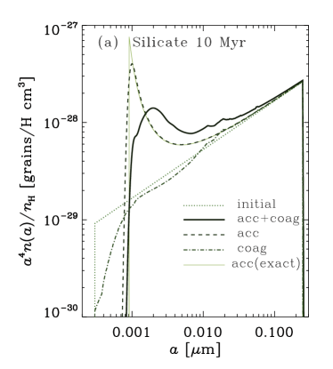
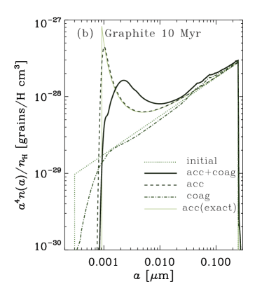
Figure 1: Grain size distributions in Model A at $t=10$ Myr. The thick solid, dashed, and dot-dashed lines show the results with both accretion and coagulation, only accretion, and only coagulation, respectively. The dotted line and the thin solid line present the initial size distribution and the analytic solution for accretion, respectively. Panels (a) and (b) show silicate and graphite, respectively.

We examine various cases, focusing on the interplay between accretion and coagulation. We fix $r$ and $a_{\mathrm{max}}$ since they do not affect the relative role between accretion and coagulation (Section 3.3). Other parameters, especially $a_{\mathrm{min}}$ and turbulent velocity, are potentially important in this paper. For convenience, we name each set of parameters Model A–D as shown in Table 2.

Table 2: Models.

Model	$r$	$a_{\mathrm{min}}$	$a_{\mathrm{max}}$	turbulence
		[nm]	[$\micron$]
A	3.5	0.3	0.25	on
B	3.5	1	0.25	on
C	3.5	0.3	0.25	off
D	3.5	1	0.25	off

In Fig. 1, we present the results for Model A at $t=10$ Myr. To show the mass distribution per logarithmic size, we multiply ${a}^{4}$ to ${n}$. Since the growth rate of grain radius, $\dot{a}$, is independent of $a$, the impact of grain growth is significant at small grain sizes. Moreover, gas-phase metals accrete selectively onto small grains because the grain surface is dominated by small grains (see also Weingartner & Draine, 1999). The results for silicate and graphite are similar because the amount of available gas-phase metals is similar.

In order to clarify the contributions from accretion and coagulation, Fig. 1 also shows the cases where either only accretion or only coagulation is taken into account in the calculation. In Fig. 1, we observe that both accretion and coagulation deplete grains at $a\la 0.001~{}\micron$. Accretion plays a significant role in increasing the grain mass around $a\sim 0.001~{}\micron$, and coagulation further pushes the peak to $a\sim 0.002~{}\micron$ at 10 Myr.

Fig. 1 also presents the analytical solution for accretion calculated by the method in HK11. Our numerical results with only accretion match the analytical solution very well except for the peak of the size distribution around $a\sim 0.001~{}\micron$. The sharp peak is smoothed because of the numerical diffusion. Reproducing the sharp peak is not important, however, since it is smoothed out by coagulation in any case.

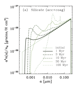
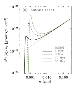
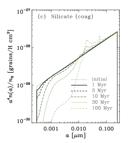
Figure 2: Same as Fig. 1 but at various $t$. The thick solid, thick dashed, dot-dashed, thin solid, and thin dashed lines show the grain size distributions at $t=1$, 3, 10, 30, and 100 Myr, respectively (in Panel b, since the grain size distributions are the same for $t\geq 10$ Myr, we do not show the size distribution at $t=100$ Myr). Each panel shows the case with (a) both accretion and coagulation, (b) only accretion, and (c) only coagulation.

Next, we show the results for Model A at various $t$ in Fig. 2. Fig. 2a presents the grain growth by accretion and coagulation. We observe continuous grain growth. The spiky features around $a\sim 0.01$–0.06 $\micron$ are produced by the accumulation of grains at sizes where the grain velocity reaches the coagulation threshold. The discrete spikes are artifact of our treatment of relative velocities, which are evaluated in a discrete way (Section 2.2). If we consider a smooth distribution of the relative direction between the grains in collision, those spiky features should be smoothed out.

To analyze the results in Fig. 2a, we examine the contribution from accretion and coagulation. We show the results for only accretion and only coagulation in Figs. 2b and c, respectively. Comparing all the panels in Fig. 2, we see that the evolution of grain size distribution is first driven by both accretion and coagulation, and is later caused by coagulation. In fact, the accretion time-scale is estimated by equation (4) as $a/\dot{a}=\tau(a)/\xi(t)$, which is $\sim 5$ Myr for $a\sim 0.001~{}\micron$ if we use the value of $\xi$ at $t=0$ ($\xi=0.3$). Coagulation of small grains also occurs on a similar time-scale. Indeed, according to equation (A5) in Hirashita & Omukai (2009), the coagulation time-scale can be estimated as $t_{\mathrm{coag}}\sim 4(n_{\mathrm{H}}/10^{3}~{}\mathrm{cm}^{-3})^{-1}(a/10^{-3}~{}\micron)^{5/2}(s/3~{}\mathrm{g~{}cm}^{-3})^{3/2}(\mathcal{D}/3\times 10^{-3})^{-1}(T/10~{}\mathrm{K})^{-1/2}$ Myr, where $\mathcal{D}$ is the dust-to-gas ratio. Although coagulation is as effective as accretion in depleting the small-sized grains, it is the role of accretion that creates the strong bump around $a\sim 0.002~{}\micron$. As we observe in Fig. 2b, accretion stops at several Myr because of the depletion of gas phase metals; thus, the evolution is purely driven by coagulation after several Myr. Comparing Figs. 2a and c, the typical grain size achieved by coagulation is not sensitive to the presence of accretion, but the bump around $\sim 0.02~{}\micron$ is stronger in the presence of accretion. Thus, accretion helps to enhance the bump, while the typical grain size reached by coagulation is not affected by accretion.

Since grain growth predominantly occurs at small sizes, it is expected that grain growth is sensitive to $a_{\mathrm{min}}$. In Fig. 3, we show the evolution of grain size distribution for Model B, in which we assume $a_{\mathrm{min}}=10$ nm instead of 3 nm. In this model, grain growth by accretion lasts 3 times longer than in Model A, because of 3 times larger $a_{\mathrm{min}}$ (note that the grain growth time-scale is proportional to $a$; equation 5). However, the growth of large grains (typically $a\ga 0.003~{}\micron$) is not affected by the change of $a_{\mathrm{min}}$.

Regardless of $a_{\mathrm{min}}$, turbulence has a significant impact on the grain size distribution at $a\ga 0.003~{}\micron$ through coagulation, especially after accretion is terminated by the depletion of gas-phase metals. In this paper, we have followed Ormel et al. (2009) for the grain motion driven by turbulence. Yan, Lazarian, & Draine (2004) show that the grain motion in magnetized turbulence can also be excited by gyroresonance. However, the grain motion in dense medium is dominated by hydrodynamical drag even in their models, and the velocities that they calculated are similar to ours for $a\la$ a few $\times 10^{-2}~{}\micron$.

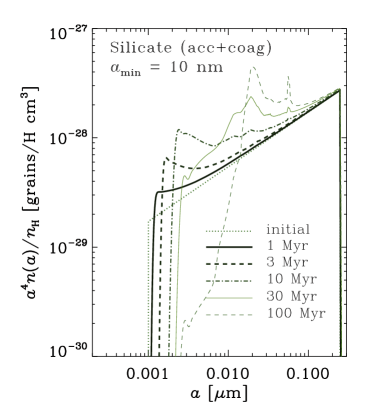
Figure 3: Same as Fig. 2a but for a larger minimum grain radius, $a_{\mathrm{min}}=1$ nm (Model B). The thick solid, thick dashed, dot-dashed, thin solid, and thin dashed lines show the cases for $t=1$, 3, 10, 30, and 100 Myr, respectively.

In order to examine the significance of turbulent motion, we also calculate the case where the turbulent velocity component is neglected; that is, $v=v_{\mathrm{th}}$ (Model C). We show the result in Fig. 4. Comparing Fig. 4 with Fig. 2a, we observe that the effect of turbulence on the grain size distribution appears after $t\sim 10$ Myr, when coagulation begins to be important for $a\ga 0.006~{}\micron$; for this grain size range, the grain motion is predominantly driven by turbulence. For $t<10~{}\mathrm{Myr}$, however, turbulence does not significantly affect the grain size distribution.

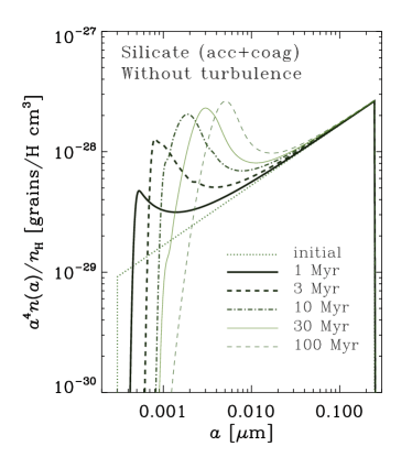
Figure 4: Same as Fig. 2a but we show the case of no turbulence (Model C).

3.2 Effect of coagulation on the grain mass growth

Grain growth by accretion in interstellar clouds is one of the most important processes that govern the grain mass budget in an entire galactic system. Following HK11, we define the increased fraction of dust mass in a cloud, $\beta$, as

$$\beta=\frac{\rho_{\mathrm{d}}(\tau_{\mathrm{cl}})}{\rho_{\mathrm{d}}(0)}-1,$$ (21)

where $\tau_{\mathrm{cl}}$ is the lifetime of clouds hosting the grain growth. The dust mass in the cloud becomes $(\beta+1)$ times as much as the initial value at the cloud lifetime, when the dust grown in the cloud returns in the diffuse ISM. By using $\beta$, the increasing rate of dust mass in a galaxy should be written as

$$\left[\frac{\mathrm{d}M_{\mathrm{dust}}}{\mathrm{d}t}\right]_{\mathrm{acc}}=\frac{\beta X_{\mathrm{cl}}M_{\mathrm{dust}}}{\tau_{\mathrm{cl}}},$$ (22)

where $M_{\mathrm{dust}}$ is the total dust mass in the galaxy, and $X_{\mathrm{cl}}$ is the mass ratio of clouds hosting the grain growth to the total gas mass (HK11).

Noting that the time-scales of accretion and coagulation are both scaled with the density of metals [$\propto(n_{\mathrm{H}}Z)^{-1}$], $\beta$ can be regarded as a function of $\tau_{\mathrm{cl}}n_{\mathrm{H}}Z$. In Fig. 5, we show $\beta$ for Models A and B to examine the dependence on grain size distribution ($a_{\mathrm{min}}=0.3$ nm and 1 nm, respectively). Because accretion occurs more efficiently at smaller grain sizes, $\beta$ is larger for $a_{\mathrm{min}}=0.3$ nm than for $a_{\mathrm{min}}=1$ nm. Accretion saturates if the metals in gas phase are used up. Thus, $\beta\to\xi(0)/[1-\xi(0)]$ if the cloud lifetime is long enough.

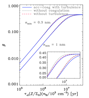
Figure 5: Increment of dust mass, $\beta$, defined in equation (21) as a function of the cloud lifetime $\tau_{\mathrm{cl}}$. To clarify the dependence on metallicity and density, the scaling with $Z$ and $n_{\mathrm{H}}$ is also shown in the horizontal axis. The difference in the upper and lower lines with the same line species is the value of $a_{\mathrm{min}}$ (0.3 nm for the upper lines and 1 nm for the lower lines). The solid, dotted, and dashed lines show the results with accretion and coagulation in the presence of turbulence, without coagulation (i.e. only accretion), and without turbulence (but with both accretion and coagulation considered), respectively. Note that the upper solid line, the upper dashed line, the lower solid line, and the lower dashed lines are equivalent to Models A, C, B, and D, respectively. In the small window, we zoom in to clarify the distinction between the lines (vertical axis is on linear scale instead of logarithmic scale).

In Fig. 5, we also plot the cases where we neglect coagulation (dotted lines). There is a slight indication that coagulation suppresses accretion. This is explained as follows: Coagulation pushes grains to larger sizes with the total volume conserved so that the surface-to-volume ratio of the grains decreases. Note that accretion rate is predominantly regulated by the surface-to-volume ratio. Nevertheless this suppression effect is very small and we can conclude that coagulation has little impact on accretion. This also means that we can neglect coagulation as long as we are interested in the total dust mass in a galaxy, although we should keep in mind that coagulation can affect the grain size distribution (Section 3.1).

Finally, we also show the case where turbulence is neglected (Models C and D) in Fig. 5. We observe that the effect of turbulence on $\beta$ is negligibly small. If $a_{\mathrm{min}}$ is larger, coagulation is very inefficient if there is no turbulent motion; thus, the grain growth without turbulence is practically the same as the grain growth without coagulation. We can also conclude that turbulence has little impact on the grain mass increase in clouds, although we should note that turbulence can affect the grain size distribution (Section 3.1).

3.3 Dependence on other parameters

We briefly discuss the influence of various parameters. The dependence of the accretion time-scale on physical quantities are clarified in equations (19) and (20). Both accretion and coagulation follow scaling of time-scale $\propto(Zn_{\mathrm{H}})^{-1}$, so that we get the same grain size distribution at the same $tZn_{\mathrm{H}}$. Precisely, the grain velocities driven by turbulence also depends on $n_{\mathrm{H}}$, but this dependence is only $\propto n_{\mathrm{H}}^{1/4}$. The time-scale of grain growth is also inversely proportional to the sticking efficiency. Regarding the gas temperature $T_{\mathrm{gas}}$, both accretion and coagulation are again regulated by the same scaling $\propto T_{\mathrm{gas}}^{-1/2}$ if coagulation is purely driven by thermal motion. Nevertheless, the gas temperature in cold gas is at most $\sim 100$ K (Wilson, Walker, & Thornley, 1997); thus, the temperature just causes a factor of 3 difference in the time-scales. Coagulation driven by turbulence is little affected by $T_{\mathrm{gas}}$, because the dependence of the turbulence-driven grain velocity on gas temperature is weak ($\propto T_{\mathrm{gas}}^{1/4}$).

As mentioned in Section 2.3, we assume that $r=3.5$. If $r$ is smaller/larger, the number of grains at the smallest sizes is smaller/larger. Thus, as already shown in HK11 (see their Fig. 3), accretion occurs more slowly/quickly. Because coagulation also occurs at the smallest grain sizes, the relative role of accretion and coagulation does not change even if we change $r$. We should note that $r=3.5$ is supported from the extinction curves in the Milky Way and Magellanic Clouds (Mathis et al., 1977; Pei, 1992). Some theoretical studies also indicate that disruption or shattering of grains in the diffuse ISM processes the grain size distribution to a power-law with $r\simeq 3.5$ (e.g. Hellyer, 1970).

As shown above, grains at $a\sim a_{\mathrm{max}}$ are not affected by accretion and coagulation. Thus, changing $a_{\mathrm{max}}$ does not affect our results. This is because both accretion and coagulation occurs efficiently for grains which have a large surface-to-volume ratio.

4 Discussion

Now we discuss two issues related to accretion and coagulation. One is effects of these processes on the extinction curve, and the other is an implication for galaxy evolution.

4.1 Effects on the extinction curve

Following Hirashita & Yan (2009) and O’Donnell & Mathis (1997), we examine how the grain size evolution affects the extinction curve. Hirashita & Yan (2009) adopt an initial condition which reproduces the Milky Way extinction curve, and incorporate the change of the grain size distribution by shattering and coagulation to examine how the extinction curve is modified by these processes. Here we examine effects of accretion and coagulation on the extinction curve.

The initial condition is set up so that the grain abundance is consistent with the mean extinction curve of the Milky Way by Pei (1992); that is, we adopt the same abundances of C and Si as listed in Table 1 but apply $\xi(0)=0.25$ and 0.15 for silicate and graphite, respectively, under Model A. This rough agreement is sufficient for our aim, since our aim is not detailed fitting of the extinction curve. We adopt the same dust optical properties and calculation method of extinction curves as in Hirashita & Yan (2009): The grain extinction cross section as a function of grain size is derived from the Mie theory, and is weighted with the grain size distribution to obtain an extinction curve.

In Fig. 6, we show the calculated extinction curves in units of magnitude per hydrogen. We present the results with both accretion and coagulation, only accretion, and only coagulation at $t=10$ Myr. First, we observe that accretion increases the grain opacity at all wavelengths because the grain mass grows. In order to examine the wavelength dependence, we also show the ratio between the extinction curve at $t=10$ Myr to that at $t=0$ Myr (initial) in the lower panel. We find that accretion ‘steepens’ the extinction curve rather than ‘flattens’ it. Naively it may be expected that the extinction curve would be flattened after accretion, because the mean grain size becomes large. Contrary to this expectation, the extinction curve becomes steeper after accretion. This is explained as follows. The extinction at a wavelength $\lambda$ is proportional to $a^{3}$ if $a\ll\lambda$, while it is proportional to to $a^{2}$ (i.e., less sensitive to the grain size) if $a\ga\lambda/(2\pi)$ (Bohren & Huffman, 1983). In other words, the ultraviolet (UV) extinction is more sensitive to the enhancement of small grains than the extinction at longer wavelengths. Therefore, the extinction at shorter wavelengths increases more sensitively as a result of accretion. The 0.22-$\micron$ bump, which is due to small graphite, also becomes more prominent after accretion. At optical and near-infrared wavelengths, the extinction is relatively insensitive compared to other wavelengths, since it is more affected by the largest grains intact after accretion and coagulation. As $\lambda$ becomes large at mid-infrared and longer wavelengths (i.e. $\lambda\gg 2\pi a_{\mathrm{max}}$), the extinction is just proportional to the grain mass (or volume).

As shown in Fig. 6 (comparison between the solid and dashed lines), coagulation flattens the UV extinction curve and lowers the carbon bump. This is because of the depletion of small grains. Coagulation conserves the total grain mass (or volume); thus, the extinction curve at $\lambda\gg 2\pi a_{\mathrm{max}}$ is unaffected by coagulation.

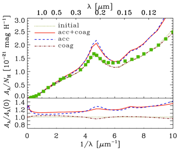
Figure 6: Upper panel: Extinction curves in units of magnitude per hydrogen. The dotted line (almost identical to the dot-dashed line) is the initial extinction curve before accretion and coagulation. The solid, dashed, and dot-dashed lines show the results with both accretion and coagulation, only accretion, and only coagulation, respectively, at $t=10$ Myr, based on the parameter sets in Model A. The filled squares represent the Galactic extinction data taken from Pei (1992). Lower Panel: The extinction divided by the initial extinction. The correspondence between the line types and the models are the same as above.

Observations of the Milky Way show that extinction curves are flatter in the directions of dense clouds (Mathis & Wallenhorst, 1981; Cardelli et al., 1989). This is not consistent with accretion, but is consistent with coagulation. Cardelli et al. (1989) also show that the extinction per hydrogen nucleus is smaller toward dense clouds than in the diffuse ISM. This requires strong coagulation. The cloud lifetime is possibly larger than 10 Myr, so that coagulation can push the grains to large sizes. Indeed, Koda et al. (2009) suggest a lifetime of $\sim 100$ Myr or longer. Another possibility of strong coagulation is that coagulation additionally occurs in extremely dense regions, e.g. regions associated with star formation (Ormel et al., 2009; Hirashita & Omukai, 2009).

4.2 Significance in galaxy evolution

Grain growth by accretion is shown to be important not only in nearby galaxies, but also in some high-redshift galaxy populations. As shown in previous studies (HK11; Inoue 2012; Asano et al. 2012), grain growth by accretion becomes prominent if the metallicity exceeds a critical value. Those studies pointed out general importance of grain growth by accretion in nearby galaxies. It is also indicated that grain growth is indeed governing the dust abundance in distant quasars (Michałowski et al., 2010; Pipino et al., 2011; Valiante et al., 2011; Asano et al., 2012) (but see Gall et al., 2011). In these objects, it is expected that coagulation is also occurring, but according to our results in this paper, the effect of coagulation on the total dust content can be neglected. If we are interested in the evolution of grain size distribution, however, we should take coagulation into account, especially after a significant fraction of gas-phase metals are locked into dust grains.

Finally, in Table 3, we briefly overview the effects of various interstellar processes on the extinction curve, including those treated in our previous papers. The carbon bump and the UV slope are enhanced by shattering (Hirashita & Yan, 2009) and accretion (this paper), while they are flattened by coagulation (Hirashita & Yan 2009; this paper) and shock destruction (Nozawa et al., 2007; Hirashita et al., 2008). We should consider at least these effects as processes determining the shape of the extinction curves observed in a variety of galaxies including high-redshift quasars and gamma-ray bursts (e.g. Gallerani et al., 2010; Jang et al., 2011, for recent observations).

Table 3: Summary of effects on the extinction curve.

Process	UV slopea	Carbon bumpb	ref.c
Accretion	$+$	$+$	1
Coagulation	$-$	$-$	1, 2
Shattering	$+$	$+$	2
Shock destruction	$-$	$-$	3

^a $+$: steeper; $-$: flatter.

^b $+$: stronger; $-$: weaker.

^c 1) this paper; 2) Hirashita & Yan (2009); 3) Hirashita et al. (2008).

5 Conclusion

In this paper, we have focused on grain growth processes in interstellar clouds. We have formulated and calculated the evolution of grain size distribution by accretion and coagulation in an interstellar cloud. Destructive processes are neglected in this paper, since they are considered to be ineffective in dense regions. We have confirmed the previous analytic results that grains smaller than $\sim 0.001~{}\micron$ are depleted by accretion on a time-scale of several Myr. Coagulation also occurs on a similar time-scale, but accretion has a prominent impact in making a large bump in the grain size distribution around $a\sim 0.001~{}\micron$ because of the grain mass increase. After a major part of the gas phase metals are used up, accretion stops and coagulation is the only mechanism that pushes the grains toward larger sizes. It is only at this stage that grain motion driven by turbulence can affect the evolution of grain size distribution. Regardless of whether accretion takes place or not, the typical grain size achieved by coagulation is similar.

We have also examined the grain mass increase during the cloud lifetime by introducing $\beta$ in equation (21) such that the grain mass becomes $(1+\beta)$ times as much as the initial value. We have found that coagulation slightly suppresses accretion although this effect is not significant and can be neglected in discussing the evolution of the total grain mass in galaxies. In other words, coagulation can be neglected in discussing the evolution of the total grain mass in galaxies.

Finally, we have investigated the effects of accretion and coagulation on the extinction curve. We have found that accretion enhances the UV slope and the carbon bump in spite of the increases in the mean grain radius. As expected, coagulation flattens these features.

Appendix A Discrete formulation

For numerical calculation, we consider $N$ discrete grain radii, and denote the lower and upper bounds of the $i$th ($i=1,\,\cdots,\,N$) bin as $a_{i-1}^{\mathrm{(b)}}$ and $a_{i}^{\mathrm{(b)}}$, respectively. We adopt $a_{i}^{\mathrm{(b)}}=a_{i-1}^{\mathrm{(b)}}\delta$, $a_{0}^{\mathrm{(b)}}=a_{\mathrm{l}}$, and $a_{N}^{\mathrm{(b)}}=a_{\mathrm{u}}$ with $\log\delta=(1/N)\log(a_{\mathrm{u}}/a_{\mathrm{l}})$. We represent the grain radius and mass in the $i$th bin with $a_{i}\equiv(a_{i-1}^{\mathrm{(b)}}+a_{i}^{\mathrm{(b)}})/2$ and $m_{i}\equiv(4\pi/3)a_{i}^{3}s$. The boundary of the mass bin is defined as $m_{i}^{\mathrm{(b)}}\equiv(4\pi/3)[a_{i}^{\mathrm{(b)}}]^{3}s$. The interval of logarithmic mass grids is denoted as $\Delta\mu=3\delta$. We also discretize the time as $t_{n}=n\Delta t$. We use integer indexes $i$ and $n$ to specify the discrete grain size and time, respectively. We adopt $N=512$, $a_{\mathrm{l}}=2\times 10^{-4}~{}\micron$, and $a_{\mathrm{u}}=0.3~{}\micron$. We apply $n(a_{0},\,t)=n(a_{N},\,t)=0$ for the boundary condition.

A.1 Accretion

Now we explain how to discretize equation (10). We denote the value of quantity $Q$ at a discrete grid as $Q_{i}^{n}$ (recall that $i$ and $n$ specify grain-size and temporal grids, respectively). Then, we obtain the following equation as a discrete version of equation (10):

$$\frac{\sigma_{i}^{n+1}-\sigma_{i}^{n}}{\Delta t}+\dot{\mu}_{i}^{n}\frac{\sigma_{i}^{n}-\sigma_{i-1}^{n}}{\Delta\mu}=\frac{1}{3}\dot{\mu}_{i}^{n}\sigma_{i}^{n},$$ (23)

where the difference is evaluated based on upwind differencing. In hydrodynamical simulations, more elaborate differencing methods have been developed, but the simple difference is enough for the grain size distribution (for example, we are not interested in ‘shocks’ or ‘instabilities’ when we are treating the grain size distribution in this paper). We apply Courant condition $\Delta t<\Delta\mu/\max_{i}(\dot{\mu}_{i}^{n})$ for every time step. From equation (11), we observe that the minimum value of $\mu$ is realized at the maximum value of $\tau(m)$, which is small when $m$ is small (equation 5). Therefore, the above Courant condition is practically evaluated at $i=1$.

Solving equation (23) for $\sigma_{i}^{n+1}$, we obtain

$$\sigma_{i}^{n+1}=\sigma_{i}^{n}\left(1-\dot{\mu}_{i}^{n}\frac{\Delta t}{\Delta\mu}+\frac{\Delta t}{3}\dot{\mu}_{i}^{n}\right)+\dot{\mu}_{i}^{n}\frac{\Delta t}{\Delta\mu}\sigma_{i-1}^{n}.$$ (24)

A.2 Coagulation

The mass density of grains contained in the $i$th bin, $\tilde{\rho}_{i}^{n}$ ($n$ is the time step), is defined as $\tilde{\rho}_{i}^{n}\equiv\sigma_{i}^{n}m_{i}\Delta\mu$. The time evolution of $\tilde{\rho}_{i}$ by coagulation can be written as

$$\frac{\tilde{\rho}_{i}^{n+1}-\tilde{\rho}_{i}^{n}}{\Delta t} = -m_{i}\tilde{\rho}_{i}\sum_{\ell=1}^{N}\alpha_{\ell i}\tilde{\rho}_{\ell}+\sum_{j=1}^{N}\sum_{\ell=1}^{N}\alpha_{\ell j}\tilde{\rho}_{\ell}\tilde{\rho}_{j}m_{\mathrm{coag}}^{\ell j}(i),$$

and

$$\alpha_{\ell k}=\left\{\begin{array}[]{ll}{\displaystyle\frac{\beta\sigma_{\ell k}v_{\ell k}}{m_{k}m_{\ell}}}&\mbox{if $v_{\ell k}<v_{\mathrm{coag}}^{\ell k}$,}\\ 0&\mbox{otherwise,}\end{array}\right.$$ (28)

where $\beta$ is the sticking probability for coagulation, and the coagulated mass $m_{\mathrm{coag}}^{\ell j}(i)$ is determined as follows: $m_{\mathrm{coag}}^{\ell j}(i)=m_{\ell}$ if $m_{i-1}^{\mathrm{(b)}}\leq m_{\ell}+m_{j}<m_{i}^{\mathrm{(b)}}$; otherwise $m_{\mathrm{coag}}^{\ell j}(i)=0$. Coagulation is assumed to occur only if the relative velocity is less than the coagulation threshold velocity $v_{\mathrm{coag}}^{\ell k}$ based on Chokshi, Tielens, & Hollenbach (1993), Dominik & Tielens (1997), and Yan et al. (2004) (see Hirashita & Yan, 2009, for further details). The cross-section for the coagulation is $\sigma_{\ell k}=\pi(a_{\ell}+a_{k})^{2}$. We assume $\beta=1$ for the sticking probability.

To confirm the validity of our numerical scheme of coagulation, we checked in Hirashita & Yan (2009) that the total dust mass is conserved. We also observe in Hirashita & Omukai (2009) that coagulation proceeds on an analytically estimated time-scale: this check is roughly equivalent with that in the appendix D of Brauer, Dullemond, & Henning (2008).

References

- Asano et al. (2012) Asano, R. S., Takeuchi, T. T., Hirashita, H., & Inoue, A. K. 2012, Earth, Planets and Space, submitted
- Bohren & Huffman (1983) Bohren, C. F., & Huffman, D. R. 1983, Absorption and Scattering of Light by Small Particles. Wiley, New York
- Brauer, Dullemond, & Henning (2008) Brauer, F., Dullemond, C. P., & Henning, Th. 2008, A&A, 480, 859
- Cardelli et al. (1989) Cardelli, J. A., Clayton, G. C., & Mathis, J. S. 1989, ApJ, 345, 245
- Cazaux & Tielens (2004) Cazaux, S., & Tielens, A. G. G. M. 2004, ApJ, 604, 222
- Chokshi, Tielens, & Hollenbach (1993) Chokshi, A., Tielens, A. G. G. M., & Hollenbach, D. 1993, ApJ, 407, 806
- Cox (2000) Cox, A. N. 2000, Allen’s Astrophysical Quantities, 4th ed., Springer, New York
- Désert, Boulanger, & Puget (1990) Désert, F.-X., Boulanger, F., & Puget, J. L. 1990, A&A, 237, 215
- Dominik & Tielens (1997) Dominik, C., & Tielens, A. G. G. M. 1997, ApJ, 480, 647
- Draine (2009) Draine, B. T. 2009, in Henning Th., Grün E., Steinacker J., eds, Cosmic Dust – Near and Far. ASP Conf. Ser., ASP, San Francisco, p. 453
- Draine & Lee (1984) Draine, B. T., & Lee, H. M. 1984, ApJ, 285, 89
- Dwek (1998) Dwek, E. 1998, ApJ, 501, 643
- Evans (1994) Evans, A. 1994, The Dusty Universe, Wiley, Chichester
- Fukui & Kawamura (2010) Fukui, Y., & Kawamura, A. 2010, ARA&A, 48, 547
- Gall et al. (2011) Gall, C., Andersen, A. C., & Hjorth, J. 2011, A&A, 528, A14
- Gallerani et al. (2010) Gallerani, S., et al. 2010, A&A, 523, A85
- Grassi et al. (2011) Grassi, T., Krstic, P., Merlin, E., Buonomo, U., Piovan, L., & Chiosi, C. 2011, A&A, 533, A123
- Hellyer (1970) Hellyer, B. 1970, MNRAS, 148, 383
- Hirashita (2000) Hirashita, H. 2000, PASJ, 52, 585
- Hirashita & Kuo (2011) Hirashita, H., & Kuo, T.-M. 2011, MNRAS, 416, 1340 (HK11)
- Hirashita & Omukai (2009) Hirashita, H., & Omukai, K. 2009, MNRAS, 399, 1795
- Hirashita et al. (2008) Hirashita, H., Nozawa, T., Takeuchi, T. T., & Kozasa, T. 2008, MNRAS, 384, 1725
- Hirashita & Yan (2009) Hirashita, H., & Yan, H. 2009, MNRAS, 394, 1061
- Inoue (2003) Inoue, A. K. 2003, PASJ, 55, 901
- Inoue (2012) Inoue, A. K. 2011, Earth, Planets, and Space, in press
- Jang et al. (2011) Jang, M., Im, M., Lee, I., Urata, Y., Huang, K., Hirashita, H., Fan, X., & Jiang, L. 2011, ApJ, 741, L20
- Jones & Nuth (2011) Jones, A. P., & Nuth, J. A., III 2011, A&A, 530, A44
- Jones et al. (1996) Jones, A. P., Tielens, A. G. G. M., & Hollenbach, D. J. 1996, ApJ, 469, 740
- Jones et al. (1994) Jones, A. P., Tielens, A. G. G. M., Hollenbach, D. J., & McKee, C. F. 1994, ApJ, 433, 797
- Koda et al. (2009) Koda, J., et al. 2009, ApJ, 700, L132
- Kozasa et al. (2009) Kozasa, T., Nozawa, T., Tominaga, N., Umeda, H., Maeda, K., & Nomoto, K. 2009, in Henning Th., Grün E., Steinacker J., eds, Cosmic Dust – Near and Far. ASP Conf. Ser., ASP, San Francisco, p. 43
- Lada, Lombardi, & Alves (2010) Lada, C. J., Lombardi, M., & Alves, J. F. 2010, ApJ, 724, 687
- Leisawitz, Bash, & Thaddeus (1989) Leisawitz, D., Bash, F. N., & Thaddeus, P. 1989, ApJS, 70, 731
- Leitch-Devlin & Williams (1985) Leitch-Devlin, M. A., & Williams, D. A. 1985, MNRAS, 213, 295
- Mathis et al. (1977) Mathis, J. S., Rumpl, W., & Nordsieck, K. H. 1977, ApJ, 217, 425
- Mathis & Wallenhorst (1981) Mathis, J. S., & Wallenhorst, S. G. 1981, ApJ, 244, 483
- McKee (1989) McKee, C. F. 1989, in Allamandola L. J. & Tielens A. G. G. M. eds., IAU Symp. 135, Interstellar Dust, Kluwer, Dordrecht, 431
- Michałowski et al. (2010) Michałowski, M. J., Murphy, E. J., Hjorth, J., Watson, D., Gall, C., & Dunlop, J. S. 2010, A&A, 522, A15
- Nozawa et al. (2007) Nozawa, T., Kozasa, T., Habe, A., Dwek, E., Umeda, H., Tominaga, N., Maeda, K., & Nomoto, K. 2007, ApJ, 666, 955
- O’Donnell & Mathis (1997) O’Donnell, J. E., & Mathis, J. S. 1997, ApJ, 479, 806
- Ormel & Cuzzi (2007) Ormel, C. W., & Cuzzi, J. N. 2007, A&A, 466, 413
- Ormel et al. (2009) Ormel, C. W., Paszun, D., Dominik, C., & Tielens, A. G. G. M. 2009, A&A, 502, 845
- Ossenkopf (1993) Ossenkopf, V. 1993, A&A, 280, 617
- Pei (1992) Pei, Y. C. 1992, ApJ, 395, 130
- Pipino et al. (2011) Pipino, A., Fan, X. L., Matteucci, F, Calura, F., Silva, L., Granato, G., & Maiolino, R. 2011, A&A, 525, A61
- Savage & Sembach (1996) Savage, B. D., & Sembach, K. R. 1996, ARA&A, 34, 279
- Spitzer (1978) Spitzer, L.1978, Physical Processes in the Interstellar Medium, Wiley, New York
- Stepnik et al. (2003) Stepnik, B., et al. 2003, A&A, 398, 551
- Valiante et al. (2009) Valiante, R., Schneider, R., Bianchi, S., & Andersen, A. C. 2009, MNRAS, 397, 1661
- Valiante et al. (2011) Valiante, R., Schneider, R., Salvadori, S., & Bianchi, S., 2011, MNRAS, 416, 1916
- Weidenschilling & Ruzmaikina (1994) Weidenschilling, S. J., & Ruzmaikina, T. V. 1994, ApJ, 430, 713
- Weingartner & Draine (1999) Weingartner, J. C., & Draine, B. T. 1999, ApJ, 517, 292
- Weingartner & Draine (2001) Weingartner, J. C., & Draine, B. T. 2001, ApJ, 548, 296
- Wilson, Walker, & Thornley (1997) Wilson, C. D., Walker, C. E., & Thornley, M. D. 1997, ApJ, 483, 210
- Yamasawa et al. (2011) Yamasawa, D., Habe, A., Kozasa, T., Nozawa, T., Hirashita, H., Umeda, H., & Nomoto, K. 2011, ApJ, 735, 44
- Yan et al. (2004) Yan, H., Lazarian, A., & Draine, B. T. 2004, ApJ, 616, 895
- Zhukovska et al. (2008) Zhukovska, S., Gail, H.-P., & Trieloff, M. 2008, A&A, 479, 453