A fast and well-conditioned spectral method

Abstract

A spectral method is developed for the direct solution of linear ordinary differential equations with variable coefficients. The method leads to matrices which are almost banded, and a numerical solver is presented that takes ${\cal O}(m^{2}n)$ operations, where $m$ is the number of Chebyshev points needed to resolve the coefficients of the differential operator and $n$ is the number of Chebyshev coefficients needed to resolve the solution to the differential equation. We prove stability of the method by relating it to a diagonally preconditioned system which has a bounded condition number, in a suitable norm. For Dirichlet boundary conditions, this implies stability in the standard $2$-norm. An adaptive QR factorization is developed to efficiently solve the resulting linear system and automatically choose the optimal number of Chebyshev coefficients needed to represent the solution. The resulting algorithm can efficiently and reliably solve for solutions that require as many as a million unknowns.

1 Introduction

Spectral methods are an important tool in scientific computing and engineering for solving differential equations (see, for instance, [6, 21, 23, 44, 45]). Although the computed solutions can converge super-algebraically to the solution of the differential equation, conventional wisdom states that spectral methods lead to dense, ill-conditioned matrices. In this paper, we introduce a spectral method which continues to converge super-algebraically to the solution, but only requires solving an almost banded, well-conditioned linear system.

Throughout, we consider the family of linear differential equations on $[-1,1]$:

$${\cal L}u=f\qquad\hbox{and}\qquad{\cal B}u={\mathbf{c}}$$ (1)

where ${\cal L}$ is an $N$th order linear differential operator

$${\cal L}u=a^{N}(x)\frac{{\mathrm{d}}^{N}u}{{\mathrm{d}}x^{N}}+\cdots+a^{1}(x)\frac{{\mathrm{d}}u}{{\mathrm{d}}x}+a^{0}(x)u,$$

${\cal B}$ denotes $K$ boundary conditions (Dirichlet, Neumann, etc.), ${\mathbf{c}}\in{\mathbb{C}}^{K}$ and $a^{0},\ldots,a^{N}$, $f$ are suitably smooth functions on $[-1,1]$. We make the assumption that the differential equation is not singular; i.e., the leading variable coefficient $a^{N}(x)$ does not vanish on the interval $[-1,1]$.

Within spectral methods there is a subdivision between collocation methods and coefficient methods; the former construct matrices operating on the values of a function at, say, Chebyshev points; the latter construct matrices operating on coefficients in a basis, say, of Chebyshev polynomials. Here there is a common belief that collocation methods are more adaptable to differential equations with variable coefficients [4, section 9.2]; i.e., when $a^{0}(x),\ldots,a^{N}(x)$ are not constant. However, the spectral coefficient method that we construct is equally applicable to differential equations with variable coefficients.

For example, the first order differential equation (chosen so the entries in the resulting linear system are integers)

$${\frac{{\mathrm{d}}u}{{\mathrm{d}}x}}+4xu=0\qquad\hbox{and}\qquad u(-1)=c,$$ (2)

results in our spectral method forming the almost banded $n\times n$ linear system

$$\left(\begin{array}[]{c c c c c c c c}1&-1&1&-1&1&-1&\cdots&(-1)^{n-1}\\[4.0pt] &2&&-1&&&&\\[4.0pt] 2&&2&&-1&&&\\[4.0pt] &1&&3&&-1&&\\[4.0pt] &&\smash{\ddots}&&\smash{\ddots}&&\smash{\ddots}&\\[4.0pt] &&&1&&n-3&&-1\\[4.0pt] &&&&1&&n-2&\\[4.0pt] &&&&&1&&n-1\\ \end{array}\right)\left(\begin{array}[]{c}u_{0}\\[4.0pt] u_{1}\\[4.0pt] u_{2}\\[4.0pt] \\[4.0pt] \smash{\vdots}\\[4.0pt] \smash{\vdots}\\[4.0pt] \\[4.0pt] u_{n-1}\end{array}\right)=\left(\begin{array}[]{c}c\\[4.0pt] 0\\[4.0pt] 0\\[4.0pt] \\[4.0pt] \smash{\vdots}\\[4.0pt] \smash{\vdots}\\[4.0pt] \\[4.0pt] 0\\ \end{array}\right).$$ (3)

We then approximate the solution to (2) as

$$u(x)=\sum_{k=0}^{n-1}u_{k}T_{k}(x)$$

where $T_{k}$ is the Chebyshev polynomial of degree $k$ (of the first kind). Moreover, the stability of solving (3) is directly related to that of a diagonally preconditioned matrix system which has $2$-norm condition number bounded above by $53.6$ for all $n$.

Our method is based on:

1. Representing derivatives in terms of ultraspherical polynomials. This results in diagonal differentiation matrices.

2. Representing conversion from Chebyshev polynomials to ultraspherical polynomials by a banded operator.

3. Representing multiplication for variable coefficients by banded operators in coefficient space. This is achieved by approximating the variable coefficients by a truncated Chebyshev (and thence ultraspherical) series.

4. Imposing the boundary conditions using boundary bordering, that is, $K$ rows of the linear system are used to impose $K$ boundary conditions. For (2), the last row of the linear system has been replaced and then permuted to the first row. This allows for a convenient solution basis to be used for general boundary conditions.

5. Using an adaptive QR decomposition to determine the optimal truncation denoted by $n_{\rm opt}$. We develop a sparse representation for the resulting dense matrix, allowing for efficient back substitution.

The resulting stable method requires only ${\cal O}(n_{\rm opt})$ operations and calculates the Chebyshev coefficients of the solution (as well as its derivatives) to machine precision. A striking application of the method is to singularly perturbed differential equations, where the bandwidth of the linear system is uniformly bounded, and the accuracy is unaffected by the extremely large condition numbers.

This paper is organized as follows. We first provide an overview of existing spectral methods. In section 2, we construct the method for first order differential equations and apply it to two problems with highly oscillatory variable coefficients. In the third section, we extend the approach to higher order differential equations by using ultraspherical polynomials, and present numerical results of the method applied to challenging second and higher-order differential equations. In the fourth section, we prove stability and convergence of the method in high order norms, which reduce to the standard $2$-norm for Dirichlet boundary conditions. In section 5, we present a fast, stable algorithm to solve the almost banded linear systems in ${\cal O}(n_{\rm opt})$ operations, where $n_{\rm opt}$ is automatically determined, allowing for the efficient solution of differential equations that require as many as a million unknowns (see Figure 8). In the final section we describe directions for future research.

Remark 1.1.

The Matlab and C++ code used for the numerical results is available from [35].

1.1 Existing techniques

Chebyshev polynomials or, more generally, Jacobi polynomials have been abundantly used to construct spectral coefficient methods. In this section we briefly survey some existing techniques.

1.1.1 Tau-method

The tau-method was originally proposed by Lanczos [28] and is analogous to representing differentiation as an operator on Chebyshev coefficients [4]. The resulting linear system, which is constructed by using recurrence relationships between Chebyshev polynomials, is always dense — even for differential equations with constant variable coefficients — and is typically ill-conditioned. The boundary conditions are imposed by replacing the last few rows of the linear system with entries constraining the solution’s coefficients.

This method was made popular and extended by Ortiz and his colleagues [23, 38] and can be made into an automated black-box solver, but this is more due to how the boundary conditions are imposed rather than the specifics of this approach. Therefore, we will use the same technique called boundary bordering for the boundary conditions.

1.1.2 Basis recombination

An alternative to boundary bordering is to impose the boundary conditions by basis recombination. That is, for our simple example (2), by computing the coefficients in the expansion

$$u(x)=cT_{0}(x)+\sum_{k=1}^{\infty}\tilde{u}_{k}\phi_{k}(x)$$

where

$$\phi_{k}(x)=\begin{cases}T_{k}(x)-T_{0}(x)&k\text{ even}\\ T_{k}(x)+T_{0}(x)&k\text{ odd}.\\ \end{cases}$$

The basis is chosen so that $\phi_{k}(-1)=0$, and there are many other possible choices.

Basis recombination runs counter to an important observation of Orszag [37]: Spectral methods in a convenient basis (like Chebyshev) can outperform an awkward problem-dependent basis. The problem-dependent basis may be theoretically elegant, but convenience is worth more in practice. In detail, the benefit of using boundary bordering instead of basis recombination include: (1) the solution is always computed in the convenient and orthogonal Chebyshev basis; (2) a fixed basis means we can automatically apply recurrence relations between Chebyshev polynomials (and later, ultraspherical polynomials) to construct multiplication matrices for incorporating variable coefficients; (3) the structure of the linear systems does not depend on the boundary condition(s), allowing for a fast, general solver; and (4) while basis recombination can result in well-conditioned linear systems, the solution can be in terms of an unstable basis for very high order boundary conditions.

There is one negative consequence of boundary bordering: it results in non-symmetric matrices — even for self-adjoint differential operators — potentially doubling the computational cost of solving the resulting linear system when using direct methods. However, our focus is on general differential equations, which are not necessarily self-adjoint.

1.1.3 Petrov–Galerkin methods

Petrov–Galerkin methods solves linear ODEs using different bases for representing the solution (trial basis) and the right-hand side of the equation (test basis). The boundary conditions determine the trial basis [31], and the boundary conditions associated to the dual differential equation can determine the test basis [41]. Shen has constructed bases for second, third, fourth and higher odd order differential equations with constant coefficients so that the resulting matrices are banded or easily invertible [17, 41, 42, 43]. Moreover, it was shown that very specific variable coefficients preserve this matrix structure [44]. These methods can be very efficient, but the method for imposing the boundary conditions is difficult to automate.

Our method will also use two different bases: the Chebyshev and ultraspherical polynomial bases. This choice preserves sparsity as do those considered in [17, 31, 41, 43], but our bases will depend on the order of the differential equation and not the boundary conditions.

1.1.4 Integral reformulation

Integral reformulation expresses the solution’s $N$th derivative in a Chebyshev expansion, solves for those coefficients before integrating back to obtain the coefficients of the solution [11, 24, 50]. The same idea was previously advocated by Clenshaw [9] and a comparison was made to the tau-method by Fox [22] who concluded that Clenshaw’s method was more accurate. In the case of constant coefficients, an alternative approach is to integrate the differential equation itself, which results in a banded system [47]. Recently, integration reformulation has received considerable attention in the literature because it can construct well-conditioned linear systems [19, 29, 47].

Clenshaw’s method was a motivating example for (F. W. J.) Olver’s algorithm [33, 30]: a method for choosing the optimal truncation parameter $n_{\rm opt}$ for calculating solutions to recurrence relationships (i.e., banded linear systems). The original paper considered dense boundary rows to handle the boundary conditions for Clenshaw’s method. In section 5.3 we develop the adaptive QR decomposition which is a generalization of Olver’s algorithm. The original approach was based on adaptive Gaussian elimination without pivoting, with a proof of numerical stability for sufficiently large $n$, but, by replacing LU with QR, we achieve stability for all $n$.

Many of the ideas that we develop in this paper are equally applicable to integral reformulation, as the resulting matrices are also almost banded. However, imposing boundary conditions requires additional variables related to the integration constants, considerably complicating the representation of multiplication. Moreover, integral reformulation does not maintain sparsity for mixed operators such as

$${{\mathrm{d}}\over{\mathrm{d}}x}a(x){{\mathrm{d}}u\over{\mathrm{d}}x},$$

as the integration will no longer annihilate the outer differentiation, which corresponds to a dense operator. Our approach avoids such issues.

1.1.5 Preconditioned iterative methods

Another approach to obtain well-conditioned linear systems is preconditioning, with the most common being motivated by a finite difference stencil [36], the operator representing the ODE with all its variable coefficients set to constants [3, 44], a finite element approximation [5, 14] or integration preconditioners [26, 20]. Once preconditioned, iterative solvers can be employed along with the Fast Fourier Transformation, which can be more efficient than dense solvers in certain situations [4, 6, 44]. While specially designed iterative methods can outperform direct methods for specific problems, they do not provide the generality and robustness that we require.

Differential equations with highly oscillatory or nonanalytic variable coefficients are one example where iterative methods may be necessary to achieve computational efficiency, as the multiplication operators have very large bandwidth in coefficient space, resulting in essentially dense linear systems. Iterative methods based on matrix-vector products avoid this growth in complexitiy, hence can be more efficient. However, the matrix-vector product has to be user-supplied code which is unlikely to be optimized in terms of memory caching or memory allocation; therefore, significant benefits over direct methods will only appear for problems that require large $n$ [49]. Moreover, direct methods provide better stability and robustness [24]. Finally, while the computational efficiency of our approach is lost for large bandwidth variable coefficients, numerical stability is maintained, as demonstrated in the second example of section 2.5.

2 Chebyshev polynomials and first order differential equations

For pedagogical reasons, we begin by solving first-order differential equations of the form

$$u^{\prime}(x)+a(x)u(x)=f(x)\qquad\hbox{and}\qquad u(-1)=c$$ (4)

where $a:[-1,1]\rightarrow\mathbb{C}$ and $f:[-1,1]\rightarrow\mathbb{C}$ are continuous functions with bounded variation. The continuity assumption ensures that (4) has a unique continuously differentiable solution on the unit interval [39], while bounded variation ensures a unique representation as a uniformly convergent Chebyshev expansion [32, Thm. 5.7]. An exact representation of a continuous function $g(x)$ with bounded variation is

$$g(x)=\sum_{k=0}^{\infty}g_{k}T_{k}(x),\hbox{ }g_{0}=\frac{2}{\pi}\int_{-1}^{1}\frac{g(x)}{\sqrt{1-x^{2}}}{\mathrm{d}}x,\hbox{ }g_{k}=\frac{1}{\pi}\int_{-1}^{1}\frac{g(x)T_{k}(x)}{\sqrt{1-x^{2}}}{\mathrm{d}}x$$ (5)

where $T_{k}(x)=\cos\left(k\cos^{-1}(x)\right)$. One way to approximate $g(x)$ is to truncate (5) after the first $n$ terms, to obtain the polynomial (of degree at most $n-1$)

$$g_{\text{trunc}}(x)=\sum_{k=0}^{n-1}g_{k}T_{k}(x).$$ (6)

The $n$ coefficients $\left\{g_{k}\right\}$ can be obtained by numerical quadrature in $\mathcal{O}(n^{2})$ operations. A second approach is to interpolate $g(x)$ at $n$ Chebyshev points — i.e., $\cos(k\pi/(n-1))$ for $k=0,1,\ldots,n-1$ — to obtain the polynomial

$$g_{\text{interp}}(x)=\sum_{k=0}^{n-1}\tilde{g}_{k}T_{k}(x).$$ (7)

In this case, the $n$ coefficients $\left\{\tilde{g}_{k}\right\}$ can be computed with a Fast Cosine Transform in just $\mathcal{O}(n\log n)$ operations. The coefficients $\left\{\tilde{g}_{k}\right\}$ and $\left\{g_{k}\right\}$ are closely related by an aliasing formula stated by Clenshaw and Curtis [10].

Usually, in practice, $g(x)$ will be many times differentiable on $[-1,1]$, and then (6) and (7) converge uniformly to $g(x)$ at an algebraic rate as $n\rightarrow\infty$. Moreover, the convergence is spectral (super-algebraic) when $g$ is infinitely differentiable, which improves to be exponential when $g$ is analytic in a neighbourhood of $[-1,1]$. If $g$ is entire, the convergence rate improves further to be super-exponential.

Mathematically, we seek the Chebyshev coefficients of the truncation (6), of $a(x)$ and $f(x)$ which are defined by the integrals (5). However, we use the coefficients in the polynomial interpolant (7) as an approximation, since the coefficients match to machine precision for sufficiently large $n$. The degree of the polynomial used to approximate $a(x)$ will later be closely related to the bandwidth of the almost banded linear system associated to (4).

The spectral method in this paper solves for the coefficients of the solution in a Chebyshev series. In order to achieve this, we need to be able to represent differentiation, $u^{\prime}(x)$, and multiplication, $a(x)u(x)$, in terms of operators on coefficients.

2.1 First order differentiation operator

The derivatives of Chebyshev polynomials satisfy

$$\frac{dT_{k}}{{\mathrm{d}}x}=\begin{cases}kC^{(1)}_{k-1}&k\geq 1\\ 0&k=0\\ \end{cases}$$ (8)

where $C^{(1)}_{k-1}(x)$ is the Chebyshev polynomial of the second kind of degree $k-1$. We use $C^{(1)}$ instead of $U$ to highlight the connection to ultraspherical polynomials, which are key to extending the method to higher order differential equations (see section 3).

Now, we use (8) to derive a simple expression for the derivative of a Chebyshev series. Suppose that $u(x)$ is given by the Chebyshev series

$$u(x)=\sum_{k=0}^{\infty}u_{k}T_{k}(x).$$ (9)

Differentiating scales the coefficients and changes the basis:

$$u^{\prime}(x)=\sum_{k=1}^{\infty}ku_{k}C^{(1)}_{k-1}(x).$$

In other words, the vector of coefficients of the derivative in a $C^{(1)}$ series is given by ${\cal D}_{0}\textbf{u}$ where ${\cal D}_{0}$ is the differentiation operator

$${\cal D}_{0}=\begin{pmatrix}0&1&\cr&&2&\cr&&&3\cr&&&&\ddots\end{pmatrix}$$

and u is the (infinite) vector of Chebyshev coefficients for $u(x)$. Note that this differentiation operator is sparse, in stark contrast to the classic differentiation operator in spectral collocation methods [4].

2.2 Multiplication operator for Chebyshev series

In order to handle variable coefficients of the form $a(x)u(x)$ in (4), we need to represent the multiplication of two Chebyshev series as an operator on coefficients. To this end, we express $a(x)$ and $u(x)$ in terms of their Chebyshev series

$$a(x)=\sum_{j=0}^{\infty}a_{j}T_{j}(x)\qquad\hbox{and}\qquad u(x)=\sum_{k=0}^{\infty}u_{k}T_{k}(x)$$

and multiply these two expressions together to obtain

$$a(x)u(x)=\sum_{j=0}^{\infty}\sum_{k=0}^{\infty}a_{j}u_{k}T_{j}(x)T_{k}(x)=\sum_{k=0}^{\infty}c_{k}T_{k}(x),$$

desiring an explicit form for $\mathbf{c}=\left(c_{0},c_{1},\ldots,\right)^{\top}$. By Proposition $2.1$ of [1] we have that

$$c_{k}=\begin{cases}a_{0}u_{0}+\frac{1}{2}\sum_{l=1}^{\infty}a_{l}u_{l}&k=0\vspace{4pt}\\ \frac{1}{2}\sum_{l=0}^{k-1}a_{k-l}u_{l}+a_{0}u_{k}+\frac{1}{2}\sum_{l=1}^{\infty}a_{l}u_{l+k}+\frac{1}{2}\sum_{l=0}^{\infty}a_{l+k}u_{l}&k\geq 1,\\ \end{cases}$$ (10)

and in terms of operators $\textbf{c}=\mathcal{M}_{0}[{a}]\textbf{u}$ where $\mathcal{M}_{0}[{a}]$ is a Toeplitz plus an almost Hankel operator given by

$$\mathcal{M}_{0}[{a}]=\frac{1}{2}\left[\begin{pmatrix}2a_{0}&a_{1}&a_{2}&a_{3}&\ldots\\ a_{1}&2a_{0}&a_{1}&a_{2}&\ddots\\ a_{2}&a_{1}&2a_{0}&a_{1}&\ddots\\ a_{3}&a_{2}&a_{1}&2a_{0}&\ddots\\ \vdots&\ddots&\ddots&\ddots&\ddots\\ \end{pmatrix}+\begin{pmatrix}0&0&0&0&\ldots\\ a_{1}&a_{2}&a_{3}&a_{4}&\iddots\\ a_{2}&a_{3}&a_{4}&a_{5}&\iddots\\ a_{3}&a_{4}&a_{5}&a_{6}&\iddots\\ \vdots&\iddots&\iddots&\iddots&\iddots\\ \end{pmatrix}\right].$$

At first glance, it appears that the multiplication operator and any truncation of it are dense. However, since $a(x)$ is continuous with bounded variation, we are able to uniformly approximate $a(x)$ with a finite number of Chebyshev coefficients to any desired accuracy. That is, for any $\epsilon>0$ there exists an $m\in\mathbb{N}$ such that

$$\left\|a(x)-\sum_{k=0}^{m-1}a_{k}T_{k}(x)\right\|_{L_{\infty}([-1,1])}<\epsilon.$$

As long as $m$ is large enough, to all practical purposes, we can use the truncated Chebyshev series to replace $a(x)$. Recall, in our implementation we approximate this truncation by the polynomial interpolant of the form (7). Hence, the $n\times n$ principal part of ${\cal M}_{0}[{a}]$ is banded with bandwidth $m$ for $n>m$. Moreover, $m$ can be surprisingly small when $a(x)$ is analytic or many times differentiable.

There is still one ingredient absent: The operator $\mathcal{D}_{0}$ returns coefficients in a $C^{(1)}$ series, whereas the operator $\mathcal{M}_{0}[{a}]$ returns coefficients in a Chebyshev series; hence, $\mathcal{D}_{0}+\mathcal{M}_{0}[{a}]$ is meaningless. In order to correct this, we require an operator that maps coefficients in a Chebyshev series to those in a $C^{(1)}$ series.

2.3 Conversion operator for Chebyshev series

The Chebyshev polynomials $T_{k}(x)$ can be written in terms of the $C^{(1)}$ polynomials by the recurrence relation

$$T_{k}=\begin{cases}\frac{1}{2}\left(C^{(1)}_{k}-C^{(1)}_{k-2}\right)&k\geq 2\vspace{2pt}\\ \frac{1}{2}C^{(1)}_{1}&k=1\vspace{2pt}\\ C^{(1)}_{0}&k=0.\end{cases}$$ (11)

A more general form of (11), which we will use later, is given in [34]. Suppose that $u(x)$ is given by the Chebyshev series (9). Then, using (11) we have

$$u(x)=\sum_{k=0}^{\infty}u_{k}T_{k}(x) =u_{0}C^{(1)}_{0}(x)+\frac{1}{2}u_{1}C^{(1)}_{1}(x)+\frac{1}{2}\sum_{k=2}^{\infty}u_{k}\left(C^{(1)}_{k}(x)-C^{(1)}_{k-2}(x)\right)$$

$$=\left(u_{0}-\frac{1}{2}u_{2}\right)C^{(1)}_{0}(x)+\sum_{k=1}^{\infty}\frac{1}{2}\left(u_{k}-u_{k+2}\right)C_{k}^{(1)}(x).$$

Hence, the $C^{(1)}$ coefficients for $u(x)$ are ${\cal S}_{0}\textbf{u}$ where ${\cal S}_{0}$ is the conversion operator

$${\cal S}_{0}=\begin{pmatrix}1&&-{\frac{1}{2}}\cr&{\frac{1}{2}}&&-{\frac{1}{2}}\cr&&{\frac{1}{2}}&&-{\frac{1}{2}}\cr&&&\ddots&&\ddots\end{pmatrix}$$

and u is the vector of Chebyshev coefficient for $u(x)$. Note that this conversion operator, and any truncation of it, is sparse and banded.

2.4 Discretization of the system

Now, we have all the ingredients to solve any differential equation of the form (4). Firstly, we can represent the differential operator as

$${\cal L}:={\cal D}_{0}+{\cal S}_{0}{\cal M}_{0}[a],$$

which takes coefficients in a Chebyshev series to those in a $C^{(1)}$ series. Due to this fact, the right-hand side $f(x)$ must be expressed in terms of its coefficients in a $C^{(1)}$ series. Hence, we can represent the differential equation (4), without its boundary conditions, as

$${\cal L}\mathbf{u}={\cal S}_{0}\mathbf{f}.$$

where $\mathbf{u}$ and $\mathbf{f}$ denote the vectors of coefficients in the Chebyshev series of the form (5) for $u(x)$ and $f(x)$, respectively.

We truncate the operators to derive a practical numerical scheme, which corresponds to applying the $n\times\infty$ projection operator given by

$${\cal P}_{n}=(I_{n},{\mathbf{0}}),$$ (12)

where $I_{n}$ is the square identity matrix of size $n$. Truncating the differentiation operator to ${\cal P}_{n}{\cal D}_{0}{\cal P}_{n}^{\top}$ results in an $n\times n$ matrix with a zero last row. This observation motivates us to impose the boundary condition by replacing the last row of ${\cal P}_{n}{\cal L}{\cal P}_{n}^{\top}$. We take the convention of permuting this boundary row to the first row so that the linear system is close to upper triangular. That is, in order to obtain an approximate solution to (4) we solve the system

$$A_{n}\left(\begin{array}[]{c}u_{0}\\ u_{1}\\ \vdots\\ u_{n-1}\end{array}\right)=\left(\begin{array}[]{c}c\vspace{15pt}\\ \left({\cal P}_{n-1}{\cal S}_{0}{\cal P}_{n}^{\top}\right)\left({\cal P}_{n}\mathbf{f}\right)\\ \vspace{4pt}\hfil\end{array}\right),$$ (13)

with

$$A_{n}=\left(\begin{array}[]{c c c c}T_{0}(-1)&T_{1}(-1)&\ldots&T_{n-1}(-1)\\ &&&\\ \lx@intercol\hfil{\cal P}_{n-1}{\cal L}{\cal P}_{n}^{\top}\hfil\lx@intercol\\ &&&\\ \end{array}\right).$$

(Note that $T_{k}(-1)=(-1)^{k}$.) The solution $u(x)$ is then approximated by the computed solution,

$$\tilde{u}(x)=\sum_{k=0}^{n-1}u_{k}T_{k}(x).$$

Remark 2.2.

Traditionally, one generates the spectral system by discretizing each operator individually; i.e., we would make the approximation

$${\cal P}_{n-1}{\cal L}{\cal P}_{n}^{\top}\approx{\cal P}_{n-1}{\cal D}_{0}{\cal P}_{n}^{\top}+\left({\cal P}_{n-1}{\cal S}_{0}{\cal P}_{n}^{\top}\right)\left({\cal P}_{n}{\cal M}[a]{\cal P}_{n}^{\top}\right).$$

However, we use can generate ${\cal P}_{n-1}{\cal L}{\cal P}_{n}^{\top}$ precisely, via

$${\cal P}_{n-1}{\cal L}{\cal P}_{n}^{\top}={\cal P}_{n-1}{\cal D}_{n}{\cal P}_{n}^{\top}+\left({\cal P}_{n-1}{\cal S}_{0}{\cal P}_{n+m}^{\top}\right)\left({\cal P}_{n+m}{\cal M}[a]{\cal P}_{n}^{\top}\right).$$

This means that each row of the operator can be generated exactly and allows us to develop the adaptive QR algorithm in section 5. Moreover, exact truncations are of critical importance for infinite dimensional linear algebra and for approximating spectra and pseudospectra [25].

2.5 Numerical examples

The traditional approach solves the linear system (13) for progressively larger $n$, and terminates the process when the tail of the solution falls below relative magnitude of machine epsilon. This is the procedure employed in Chebfun [46, 18] and results in ${\cal O}(n_{\rm opt}\log n_{\rm opt})$ complexity. Instead the adaptive QR algorithm of section 5 can be used to find the optimal truncation and solve for the solution, concurrently which reduces the complexity to just ${\cal O}(n_{\rm opt})$.

For the first example, we consider the linear differential equation

$$u^{\prime}(x)+x^{3}u(x)=100\sin\left(20,\!000x^{2}\right)\qquad u(-1)=0$$ (14)

which has a highly oscillatory forcing term. The exact solution is

$$u(x)=e^{-\frac{x^{4}}{4}}\left(\int_{-1}^{x}100e^{\frac{t^{4}}{4}}\sin\left(20,\!000t^{2}\right)dt\right).$$

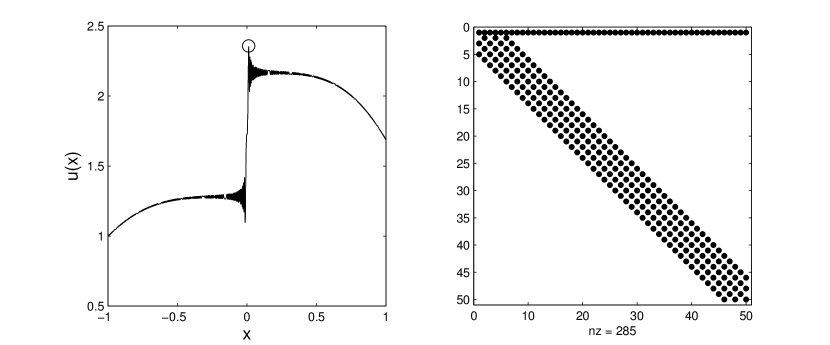
Fig. 1: Left: The highly oscillatory solution to (14) with the maximum of the solution computed and marked by a circle. Right: Sparsity structure of the almost banded linear system, with the number of non-zero entries denoted by nz.

The computed solution is a polynomial of degree $20,\!391$ and uniformly approximates the exact solution to essentially machine precision. The computed solution is of very high degree because at least $2$ coefficients are required per oscillation — the Nyquist rate. In Figure 1 we plot the computed oscillatory solution, and a realization of the matrix when $n=50$, which shows the almost banded structure of the linear system.

The approximate solution is expressed in terms of a Chebyshev basis, which is convenient for further manipulation. For example, its maximum is $2.3573$ (circled in Figure 1), its integral is $3.2879$ and the equation $u(x)-1.3=0$ has $113$ solutions in $x\in[-1,1]$.

As a second example we consider the linear differential equation

$$u^{\prime}(x)+\frac{1}{ax^{2}+1}u(x)=0\qquad\hbox{and}\qquad u(-1)=1.$$ (15)

We take $a=5\times 10^{4}$, in which case the variable coefficient can be approximated to roughly machine precision by a polynomial of degree $7,\!350$, and hence, only for very large $n$ is the linear system (13) banded.

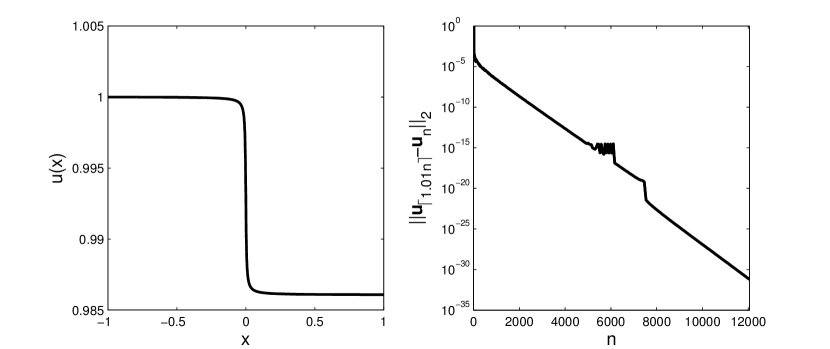
Fig. 2: Left: The computed solution to (15) with $a=5\times 10^{4}$. Right: Plot of the Cauchy error for the solution coefficients, which shows the 2-norm difference between the coefficients of the approximate solution when solving an $n\times n$ and an $\lceil 1.01n\rceil\times\lceil 1.01n\rceil$ matrix system.

The exact solution to (15) is

$$u(x)=\exp\left(-\frac{\tan^{-1}(\sqrt{a}x)+\tan^{-1}(\sqrt{a})}{\sqrt{a}}\right),$$

which can be approximated to machine precision by a polynomial of degree $5,\!377$, determined by interpolating at Chebyshev points. On the other hand, the computed solution $\tilde{u}(x)$, is a polynomial of degree $5,\!093$ such that

$$\left(\int_{-1}^{1}\left(u(x)-\tilde{u}(x)\right)^{2}{\mathrm{d}}x\right)^{\frac{1}{2}}=2.86\times 10^{-15}.$$

The solution contains a thin boundary layer and contains a singularity in the complex plane which is close in proximity to the $[-1,1]$. This means that the associated Berstein ellipse is restricted and therefore, a large degree polynomial is required to approximate the solution (see, for example, [12]). A plot of the solution and the Cauchy error are included in Figure 2. The Cauchy error plot confirms that the solution is, up to machine precision, independent of the number of coefficients in its expansion for $n\geq 5,\!100$.

3 Ultraspherical polynomials and high order differential equations

We now generalize the approach to high order differential equations of the form

$$\sum_{\lambda=0}^{N}a^{\lambda}(x)\frac{{\mathrm{d}}^{\lambda}u(x)}{{\mathrm{d}}x^{\lambda}}=f(x)\hskip 28.45274pt\text{on }[-1,1],$$ (16)

with general boundary conditions ${\cal B}u=\mathbf{c}$. We assume that the boundary operator ${\cal B}$ is given in terms of the Chebyshev coefficients of $u$. For example, for Dirichlet conditions

$${\cal B}=\begin{pmatrix}T_{0}(-1)&T_{1}(-1)&T_{2}(-1)&\cdots\\ T_{0}(1)&T_{1}(1)&T_{2}(1)&\cdots\end{pmatrix}=\begin{pmatrix}1&-1&1&-1&\cdots\\ 1&1&1&1&\cdots\end{pmatrix},$$

and for Neumann conditions

$${\cal B}=\begin{pmatrix}T_{0}^{\prime}(-1)&T_{1}^{\prime}(-1)&T_{2}^{\prime}(-1)&\cdots\\ T_{0}^{\prime}(1)&T_{1}^{\prime}(1)&T_{2}^{\prime}(1)&\cdots\end{pmatrix}=\begin{pmatrix}0&1&-4&\cdots&(-1)^{k+1}k^{2}&\cdots\\ 0&1&4&\cdots&k^{2}&\cdots\end{pmatrix}.$$

We can also impose less standard boundary conditions; e.g., we can impose that the solution integrates to a constant by using the Clenshaw–Curtis weights [10] (computable in ${\cal O}(n\log n)$ operations [48]) or it evaluates to a fixed constant in $(-1,1)$. In fact, because we are using boundary bordering, any boundary condition which depends linearly on the solution’s coefficients can be imposed in an automated manner.

The approach of the first order method relied on three relations: differentiation (8), multiplication (10) and conversion (11). To generalize the spectral method to higher order differential equations we use similar relations, now in terms of higher order ultraspherical polynomials.

The ultraspherical (or Gegenbauer) polynomials $C_{0}^{(\lambda)}(x),C_{1}^{(\lambda)}(x),\ldots$ are a family of polynomials orthogonal with respect to the weight

$$(1-x^{2})^{\lambda-\frac{1}{2}}.$$

We will only use ultraspherical polynomials for $\lambda=1,2,\ldots$, defined uniquely by normalizing the leading coefficient so that

$$C_{k}^{(\lambda)}(x)=\frac{2^{k}(\lambda)_{k}}{k!}x^{k}+{\cal O}(x^{k-1}),$$

where $(\lambda)_{k}=\frac{(\lambda+k-1)!}{(\lambda-1)!}$ denotes the Pochhammer symbol. In particular, the ultraspherical polynomials with $\lambda=1$ are the Chebyshev polynomials of the second kind, which we denote by $C^{(1)}$.

Importantly, ultraspherical polynomials satisfy an analogue of (8) [34],

$$\frac{dC_{k}^{(\lambda)}}{{\mathrm{d}}x}=\begin{cases}2\lambda C_{k-1}^{(\lambda+1)}&k\geq 1\\ 0&k=0.\\ \end{cases},\qquad\lambda\geq 1.$$ (17)

Moreover, they also satisfy an analogue to (11)

$$C_{k}^{(\lambda)}=\begin{cases}\frac{\lambda}{\lambda+k}\left(C_{k}^{(\lambda+1)}-C_{k-2}^{(\lambda+1)}\right)&k\geq 2\\ \frac{\lambda}{\lambda+1}C_{1}^{(\lambda+1)}&k=1\\ C_{0}^{(\lambda+1)}&k=0,\\ \end{cases}\qquad\lambda\geq 1.$$ (18)

Suppose that $u(x)$ is represented as the Chebyshev series (9). Then, for $\lambda=1,2,\ldots$, (8) implies that

$$\frac{{\mathrm{d}}^{\lambda}u(x)}{{\mathrm{d}}x^{\lambda}}=\sum_{k=1}^{\infty}ku_{k}\frac{{\mathrm{d}}^{\lambda-1}C^{(1)}_{k-1}(x)}{{\mathrm{d}}x^{\lambda-1}}.$$

By applying the relation (17) $\lambda-1$ times we obtain

$$\frac{{\mathrm{d}}^{\lambda}u(x)}{{\mathrm{d}}x^{\lambda}}=2^{\lambda-1}(\lambda-1)!\sum_{k=\lambda}^{\infty}ku_{k}C^{(\lambda)}_{k-\lambda}(x).$$

This means that the $\lambda$-order differentiation operator takes the form

$$\mathcal{D}_{\lambda}=2^{\lambda-1}(\lambda-1)!\begin{pmatrix}\overbrace{0\quad\cdots\quad 0}^{\mbox{$\lambda$ times}}&\lambda&&&\\ &&\lambda+1&\\ &&&\lambda+2&\\ &&&&\ddots\\ \end{pmatrix}.$$

The $\lambda$-order differentiation operator that does not change bases can be constructed from recurrence relations [16] and this can be used to construct spectral methods [15]. However, the differentiation operator is not sparse.

In the process of differentiation ${\cal D}_{\lambda}$ converts coefficients in a Chebyshev series to coefficients in a $C^{(\lambda)}$ series. Moreover, using (18) the operator which converts coefficients in $C^{(\lambda)}$ series to those in a $C^{(\lambda+1)}$ series is given by

$${\cal S}_{\lambda}=\begin{pmatrix}1&&-\frac{\lambda}{\lambda+2}&&\\ &\frac{\lambda}{\lambda+1}&&-\frac{\lambda}{\lambda+3}&\\ &&\frac{\lambda}{\lambda+2}&&-\frac{\lambda}{\lambda+4}&\\ &&&\ddots&&\ddots\\ \end{pmatrix}.$$

As before, we also require a multiplication operator, but this time representing the multiplication between two $C^{(\lambda)}$ ultraspherical series.

3.1 Multiplication operator for ultraspherical series

In order to handle the variable coefficients in (16), we must represent multiplication of two ultraspherical series in coefficient space. Given two functions

$$a(x)=\sum_{j=0}^{\infty}a_{j}C^{(\lambda)}_{j}(x)\qquad\hbox{and}\qquad u(x)=\sum_{k=0}^{\infty}u_{k}C^{(\lambda)}_{k}(x),$$

we have

$$a(x)u(x)=\sum_{j=0}^{\infty}\sum_{k=0}^{\infty}a_{j}u_{k}C^{(\lambda)}_{j}(x)C^{(\lambda)}_{k}(x).$$ (19)

To obtain a $C^{(\lambda)}$ series for $a(x)u(x)$ we use the linearization formula given by Carlitz [7], which takes the form

$$C_{j}^{(\lambda)}(x)C_{k}^{(\lambda)}(x)=\sum_{s=0}^{\min(j,k)}c^{\lambda}_{s}(j,k)C_{j+k-2s}^{(\lambda)}(x)$$ (20)

where

$$c^{\lambda}_{s}(j,k)=\frac{j+k+\lambda-2s}{j+k+\lambda-s}\frac{(\lambda)_{s}(\lambda)_{j-s}(\lambda)_{k-s}}{s!(j-s)!(k-s)!}\frac{(2\lambda)_{j+k-s}}{(\lambda)_{j+k-s}}\frac{(j+k-2s)!}{(2\lambda)_{j+k-2s}}$$ (21)

and $(\lambda)_{k}=\frac{(\lambda+k-1)!}{(\lambda-1)!}$ is the Pochhammer symbol. We substitute (20) into (19) and rearrange the summation signs to obtain

$$a(x)u(x)=\sum_{j=0}^{\infty}\left(\sum_{k=0}^{\infty}\sum_{s=\max(0,k-j)}^{k}a_{2s+j-k}c^{\lambda}_{s}(k,2s+j-k)u_{k}\right)C_{j}^{(\lambda)}(x).$$ (22)

From (22) the $(j,k)$ entry of the multiplication operator representing the product of $a(x)$ in a $C^{(\lambda)}$ series is

$${\cal M}_{\lambda}[a]_{j,k}=\sum_{s=\max(0,k-j)}^{k}a_{2s+j-k}c^{\lambda}_{s}(k,2s+j-k),\hskip 28.45274ptj,k\geq 0.$$

In practice, $a(x)$ will be approximated by a truncation of its $C^{(\lambda)}$ series,

$$a(x)\approx\sum_{j=0}^{m-1}a_{j}C^{(\lambda)}_{j}(x),$$ (23)

and with this approximation the matrix ${\cal P}_{n}{\cal M}_{\lambda}[a]{\cal P}_{n}^{\top}$ is banded with bandwidth $m$ for $n>m$. The expansion (23) can be computed by approximating the first $m$ Chebyshev coefficients in the Chebyshev series for $a(x)$ and then applying a truncation of the conversion operator ${\cal S}_{\lambda-1}\cdots S_{0}$.

The formula for $c_{s}^{\lambda}(j,k)$, (21), cannot be used directly to form ${\cal M}_{\lambda}[a]$ due to arithmetic overflow issues that arise for $j,k\geq 70$. Instead, we cancel terms in the numerator and denominator of (21) and match up the remaining terms of similar magnitude to obtain an equivalent, but more numerically stable formula

$$c^{\lambda}_{s}(j,k) = \frac{j+k+\lambda-2s}{j+k+\lambda-s}\times\prod_{t=0}^{s-1}\frac{\lambda+t}{1+t}\times\prod_{t=0}^{j-s-1}\frac{\lambda+t}{1+t}$$ (24)

$$\times \prod_{t=0}^{s-1}\frac{2\lambda+j+k-2s+t}{\lambda+j+k-2s+t}\times\prod_{t=0}^{j-s-1}\frac{k-s+1+t}{k-s+\lambda+t}.$$

All the fractions are of magnitude $\mathcal{O}(1)$ in size, and hence ${\cal P}_{n}{\cal M}_{\lambda}[a]{\cal P}_{n}^{\top}$ can be formed in floating point arithmetic. For the purposes of computational speed, we only apply (24) once per entry, and use the recurrence relation

$$c^{\lambda}_{s+1}(j,k+2)=c^{\lambda}_{s}(j,k) \times \frac{j+k+\lambda-s}{j+k+\lambda-s+1}\times\frac{\lambda+s}{s+1}\times$$

$$\times \frac{j-s}{\lambda+j-s-1}\times\frac{2\lambda+j+k-s}{\lambda+j+k-s}\times\frac{k-s+\lambda}{k-s+1}$$

to generate all the other terms required.

Remark 3.3.

In the special case when $\lambda=1$, the multiplication operator ${\cal M}_{1}[a]$ can be decomposed as a Toeplitz operator plus a Hankel operator.

3.2 Discretization of the system

We now have everything in place to be able to solve high order differential equations of the form (16). Firstly, we can represent the differential operator as

$${\cal L}:={\cal M}_{N}[a^{N}]{\cal D}_{N}+\sum_{\lambda=1}^{N-1}{\cal S}_{N-1}\cdots{\cal S}_{\lambda}{\cal M}_{\lambda}[a^{\lambda}]{\cal D}_{\lambda}+{\cal S}_{N-1}\cdots{\cal S}_{0}{\cal M}_{0}[a^{0}],$$

which takes coefficients in a Chebyshev series to those in a $C^{(N)}$ series. Due to this fact, the right hand side $f(x)$ must be expressed in terms of its coefficients in a $C^{(N)}$ series. Moreover, we impose the $K$ boundary conditions on the solution by replacing the last $K$ rows of ${\cal P}_{n}{\cal L}{\cal P}_{n}^{\top}$ and permute these to the first $K$ rows. That is, in order to obtain an approximate solution to (16) we solve the system

$$A_{n}\left(\begin{array}[]{c}u_{0}\\ u_{1}\\ \vdots\\ u_{n-1}\end{array}\right)=\left(\begin{array}[]{c}\mathbf{c}\vspace{15pt}\\ {\cal P}_{n-K}{\cal S}_{N-1}\cdots{\cal S}_{0}\mathbf{f}\\ \vspace{4pt}\hfil\end{array}\right),$$

where

$$A_{n}=\begin{pmatrix}\mathcal{B}{\cal P}_{n}^{\top}\\ \\ {\cal P}_{n-K}{\cal L}{\cal P}_{n}^{\top}\\ \\ \end{pmatrix}$$

and $\mathbf{f}$ is again a vector containing the Chebyshev coefficients of the right-hand side $f$. The solution $u(x)$ is then approximated by the $n$-term Chebyshev series:

$$u(x)\approx\sum_{k=0}^{n-1}u_{k}T_{k}(x).$$

3.3 Numerical examples

For the first example we consider the Airy differential equation

$$\epsilon u^{\prime\prime}(x)-xu(x)=0\qquad\text{with}\qquad u(-1)={\text{Ai}}\left(-\sqrt[3]{\frac{1}{\epsilon}}\right),\text{ }u(1)={\text{Ai}}\left(\sqrt[3]{\frac{1}{\epsilon}}\right)$$ (25)

where ${\text{Ai}}(\cdot)$ is the Airy function of the first kind.

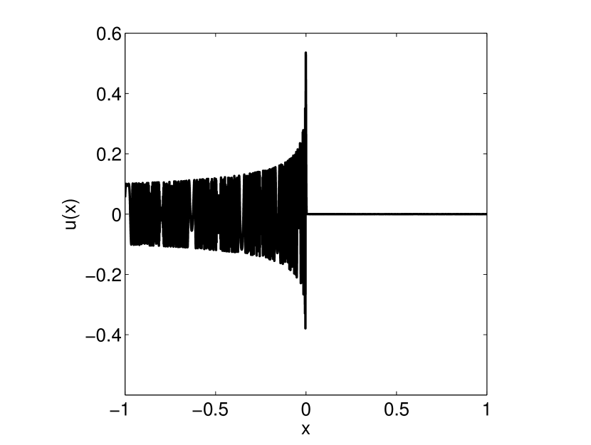
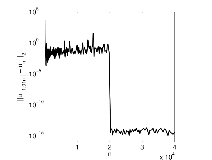
Fig. 3: Left: The highly oscillatory solution to (25) with $\epsilon=10^{-9}$. Right: The Cauchy error for the solution coefficients. The plot shows the 2-norm difference between the coefficients of the approximate solution when solving an $n\times n$ and $\lceil 1.01n\rceil\times\lceil 1.01n\rceil$ matrix system.

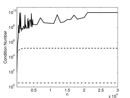
Fig. 4: Plot of the condition number of the linear systems to solve (25) against the size of the discretization, for $\epsilon=1\times 10^{-9}$ (solid), $\epsilon=1\times 10^{-4}$ (dashed) and $\epsilon=1$ (dot-dashed). For $\epsilon=1$ we employ the diagonal preconditioner presented in section 4. The plot demonstrates that the $2$-norm condition number is bounded from above. The observed error in the solution is considerably better than what is suggested by the bounding constants, as seen in Fig. 3.

In Figure 3 we take $\epsilon=10^{-9}$ and plot the computed solution which is a polynomial of degree $20,\!003$. The exact solution to (25) is the scaled Airy function,

$$u(x)={\text{Ai}}\left(\sqrt[3]{\frac{1}{\epsilon}}x\right).$$

Letting $\tilde{u}(x)$ denote the computed solution, we have

$$\left(\int_{-1}^{1}\left(u(x)-\tilde{u}(x)\right)^{2}\right)^{1/2}=2.44\times 10^{-12}$$

which is surprisingly good when compared with the ill-conditioning inherent in this singularly perturbed differential equation. Numerically we witness that the spectral method delivers much better accuracy than standard bounds based on the condition number would suggest. The Cauchy error plot in Figure 3 indicates that the solution coefficients themselves are resolved to essentially machine precision, for $n\geq 20,\!000$. In Figure 4 we show numerical evidence that with a simple diagonal preconditioner, which we analysis in the next section the condition number of the linear systems formed are bounded for all $n$. Later, for $\epsilon=1$, we also show in Figure 9 that the derivatives of the solution are well approximated.

For the second example we consider the boundary layer problem,

$$\epsilon u^{\prime\prime}(x)-2x\left(\cos(x)-\frac{8}{10}\right)u^{\prime}(x)+\left(\cos(x)-\frac{8}{10}\right)u(x)=0$$ (26)

with boundary conditions

$$u(-1)=u(1)=1.$$

Perturbation theory shows that the solution has two boundary layers at $\pm\cos^{-1}(8/10)$ both of width ${\cal O}(\epsilon^{1/4})$. In Figure 5 we take $\epsilon=10^{-7}$. The computed solution is of degree $15,\!394$ and it is confirmed by the Cauchy error plot that the solution is well-resolved.

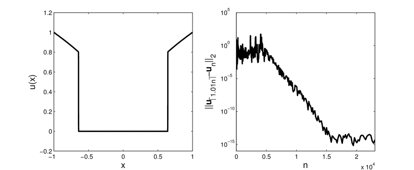
Fig. 5: Left: The solution to the boundary layer problem (26) with $\epsilon=10^{-7}$. Right: The Cauchy error in the $2$-norm for the solution coefficients.

For the last example we consider the high order differential equation

$$u^{(10)}(x)+\cosh(x)u^{(8)}(x)+x^{2}u^{(6)}(x)+x^{4}u^{(4)}(x)+\cos(x)u^{(2)}(x)+x^{2}u(x)=0$$

with boundary conditions

$$u(-1)=u(1)=0,\text{ }u^{\prime}(-1)=u^{\prime}(1)=1,\text{ }u^{(k)}(\pm 1)=0,\text{ }2\leq k\leq 4.$$

This is far from a practical example, and an exact solution seems difficult to construct. Instead, we note that if $u(x)$ is the solution then it is odd; that is, $u(x)=-u(-x)$. Our method does not impose such a condition and therefore, we can use it along with the Cauchy error to gain confidence in the computed solution. The computed solution $\tilde{u}(x)$ is of degree $55$ and plotted in Figure 6. Moreover, the computed solution is odd to about machine precision,

$$\left(\int_{-1}^{1}\left(\tilde{u}(x)+\tilde{u}(-x)\right)^{2}\right)^{1/2}=1.252\times 10^{-14}.$$

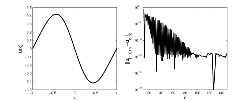
Fig. 6: Left: Plot of the solution to the $10$th order differential equation. Right: Plot of the Cauchy error in the $2$-norm for the solution coefficients.

4 Stability and convergence

The $2$-norm condition number of a matrix $A\in\mathbb{C}^{n\times n}$ is defined as

$$\kappa(A)=\left\|A\right\|_{2}\left\|A^{-1}\right\|_{2}.$$

Without any preconditioning $\kappa\!\begin{pmatrix}A_{n}\end{pmatrix}$ grows proportionally with $n$, which is significantly better than the typical growth of ${\cal O}(n^{2N})$ in the condition number for the standard tau and collocation methods (see section $4.3$ of [6]). However, the accuracy seen in practice even outperforms this: the backward error is consistent with a numerical method with bounded condition number. Later, we will show that a trivial, diagonal preconditioner that scales the columns results in a linear system with a bounded condition number. However, we observe that even without preconditioning the linear systems can be solved to the same accuracy. We explain this with the following proposition that the stability of QR is not affected by column scaling.

Proposition 4.4.

Suppose $R$ is a diagonal matrix. Solving $A\mathbf{c}=\mathbf{b}$ using QR (with Givens rotations) is stable if QR applied to solve $AR\mathbf{q}=\mathbf{b}$ is stable and $\|R\|_{\infty}\leq 1$.

Proof 4.5.

This follows immediately from the invariance of Givens rotations to column scaling and the stability of back substitution, see [27, pp. 374].

4.1 A diagonal preconditioner and compactness

Through-out this section we assume that $a^{N}(x)=1$ (otherwise, divide through by the coefficient on the highest order term, assuming it is nonsingular). We make the restriction that $K=N$; that is, the $N$th order differential equation has exactly $N$ boundary conditions. When $K>N$ it is more appropriate to choose a non-diagonal preconditioner, but we do not analyse that situation here.

We show that there exists a diagonal preconditioner so that the preconditioned system has bounded condition number in high order norms (Definition 4.6). For Dirichlet boundary conditions the preconditioned system has bounded condition number in the $2$-norm.

Define the diagonal preconditioner by,

$${\cal R}=\frac{1}{2^{N-1}(N-1)!}\text{diag}\Bigl{(}\overbrace{1,\ldots,1}^{\mbox{$N$ times}},\frac{1}{N},\frac{1}{N+1},\ldots\Bigr{)}.$$

In practice, we observe that many other diagonal preconditioners also give a bounded condition number and it is likely that there are preconditioners which give better practical bounds on the backward error, but only by a constant factor.

The analysis of $(\ref{ODE})$ will follow from the fact that, on suitably defined spaces,

$$\begin{pmatrix}\mathcal{B}\\ \mathcal{L}\\ \end{pmatrix}{\cal R}=I+{\cal K},$$

for a compact operator ${\cal K}$, where $\mathcal{L}$ is the $N$th order differential operator and $\mathcal{B}$ is a boundary operator representing $N$ boundary conditions. To this aim, we need to be precise on which spaces these operators act on. Since we are working in coefficient space, we will consider the problems as defined in $\ell_{\lambda}^{2}$ spaces:

Definition 4.6.

The space $\ell_{\lambda}^{2}\subset{\mathbb{C}}^{\infty}$ is defined as the Banach space with norm

$$\|{\mathbf{u}}\|_{\ell^{2}_{\lambda}}=\sqrt{\sum_{k=0}^{\infty}|u_{k}|^{2}(k+1)^{2\lambda}}<\infty.$$

We now show that the preconditioned operator is a compact perturbation of the identity.

Lemma 4.7.

Suppose that the boundary operator $\mathcal{B}:\ell^{2}_{D}\rightarrow{\mathbb{C}}^{K}$ is bounded. Then

$$\begin{pmatrix}\mathcal{B}\\ \mathcal{L}\\ \end{pmatrix}{\cal R}=I+{\cal K}$$

where ${\cal K}:\ell^{2}_{\lambda}\rightarrow\ell^{2}_{\lambda}$ is compact for $\lambda=D-1,D,\ldots$.

Proof 4.8.

Firstly, note that

$$\begin{pmatrix}{\cal B}\cr{\cal L}\end{pmatrix} =\begin{pmatrix}2^{N-1}(N-1)!{\cal P}_{N}\cr{\cal D}_{N}\end{pmatrix}+\begin{pmatrix}{\cal B}-2^{N-1}(N-1)!{\cal P}_{N}\cr 0\end{pmatrix}$$

$$+\begin{pmatrix}0\cr{\cal S}_{N-1}{\cal M}_{N-1}{[a^{N-1}]}{\cal D}_{N-1}+\cdots+{\cal S}_{N-1}\cdots{\cal S}_{1}{\cal M}_{1}{[a^{1}]}{\cal D}+{\cal S}_{N-1}\cdots{\cal S}_{0}{\cal M}{[a^{0}]}\end{pmatrix}$$

where ${\cal P}_{N}:\ell^{2}_{\lambda}\rightarrow{\mathbb{C}}^{N}$ is the $N\times\infty$ projection operator (12).

Secondly, we remark that ${\cal R}:\ell^{2}_{\lambda}\rightarrow\ell^{2}_{\lambda+1}$ and hence, ${\cal B}{\cal R}:\ell^{2}_{\lambda}\rightarrow{\mathbb{C}}^{N}$ is bounded for $\lambda=D-1,D,\ldots$. Furthermore, ${\cal S}_{k}:\ell^{2}_{\lambda}\rightarrow\ell^{2}_{\lambda+1}$ is bounded for $k=1,2,\ldots$ and so is, ${\cal D}_{N}:\ell^{2}_{\lambda}\rightarrow\ell^{2}_{\lambda-1}$. It follows that

$$\begin{pmatrix}2^{N-1}(N-1)!{\cal P}_{N}\cr{\cal D}_{N}\end{pmatrix}{\cal R}=I:\ell^{2}_{\lambda}\rightarrow\ell^{2}_{\lambda}.$$

Since $\begin{pmatrix}{\cal B}-2^{N-1}(N-1)!{\cal P}_{N}\cr 0\end{pmatrix}{\cal R}:\ell^{2}_{\lambda}\rightarrow\ell^{2}_{\lambda}$ for $\lambda=D-1,D,\ldots$ is bounded and has finite rank, it is compact. Note that ${\cal R}$ is compact as an operator ${\cal R}:\ell^{2}_{\lambda}\rightarrow\ell^{2}_{\lambda}$, as are ${\cal S}_{N-1},\ldots,{\cal S}_{1}$ (since ${\cal S}_{k}{\cal R}^{-1}:\ell^{2}_{\lambda}\rightarrow\ell^{2}_{\lambda}$ are bounded and ${\cal R}$ is compact). It follows that the last term

$$\begin{pmatrix}0\cr{\cal S}_{N-1}\cdots{\cal S}_{0}{\cal M}{[a^{0}]}\end{pmatrix}{\cal R}:\ell^{2}_{\lambda}\rightarrow\ell^{2}_{\lambda}$$

is compact, since ${\cal M}[a^{0}]$ and ${\cal S}_{0}$ are also bounded. Finally, each of the intermediate terms are compact since $\begin{pmatrix}0\cr{\cal D}_{k}\end{pmatrix}{\cal R}:\ell^{2}_{\lambda}\rightarrow\ell^{2}_{\lambda}$ is bounded and ${\cal S}_{k}$ are compact.

We have shown that the preconditioned operator is the identity plus a sum of compact operators and hence a compact perturbation of the identity.

The compactness of ${\cal K}$ allows us to show well-conditioning and convergence.

Lemma 4.9.

Suppose that $\begin{pmatrix}{\cal B}\cr{\cal L}\end{pmatrix}:\ell^{2}_{\lambda+1}\rightarrow\ell^{2}_{\lambda}$ is an invertible operator for some $\lambda\in\{D-1,D,\ldots\}$. Then, as $n\rightarrow\infty$,

$$\|A_{n}R_{n}\|_{\ell^{2}_{\lambda}}={\cal O}(1)\hbox{ and }\|{(A_{n}R_{n})^{-1}}\|_{\ell^{2}_{\lambda}}={\cal O}(1),$$

for the diagonal matrix $R_{n}={\cal P}_{n}{\cal R}{\cal P}_{n}^{\top}$ and truncated spectral matrix

$$A_{n}={\cal P}_{n}\begin{pmatrix}{\cal B}\\ {\cal L}\end{pmatrix}{\cal P}_{n}^{\top}.$$

Proof 4.10.

Since ${\cal R}:\ell^{2}_{\lambda}\rightarrow\ell^{2}_{\lambda+1}$ is invertible, we have that $I+{\cal K}:\ell^{2}_{\lambda}\rightarrow\ell^{2}_{\lambda}$ is invertible. The lemma follows since ${\cal K}$ is compact,

$$A_{n}R_{n}={\cal P}_{n}(I+{\cal K}){\cal R}^{-1}{\cal P}_{n}^{\top}{\cal P}_{n}{\cal R}{\cal P}_{n}^{\top}=I_{n}+{\cal P}_{n}{\cal K}{\cal P}_{n}^{\top},$$

and ${\cal P}_{n}^{\top}{\cal P}_{n}{\cal K}{\cal P}_{n}^{\top}{\cal P}_{n}$ converges in norm to ${\cal K}$.

4.2 Convergence

Denote the coefficients of the exact solution by $\mathbf{u}$, and note that vector $\mathcal{P}_{n}^{\top}\mathcal{P}_{n}\mathbf{u}$ agrees with $\mathbf{u}$ for the first $n$ coefficients and thereafter has zero entries. We show that our numerical scheme converges at the same rate as $\mathcal{P}_{n}^{\top}\mathcal{P}_{n}\mathbf{u}$ converges to $\mathbf{u}$.

Theorem 4.11.

Suppose $\mathbf{f}\in\ell^{2}_{\lambda-N+1}$ for some $\lambda\in\{D-1,D,\ldots\}$, and that $\begin{pmatrix}{\cal B}\cr{\cal L}\end{pmatrix}:\ell^{2}_{\lambda+1}\rightarrow\ell^{2}_{\lambda}$ is an invertible operator. Define

$${\mathbf{u}}_{n}=A_{n}^{-1}{\cal P}_{n}\begin{pmatrix}\mathbf{c}\cr{\cal S}_{N-1}\cdots{\cal S}_{0}\mathbf{f}\end{pmatrix}.$$

Then

$$\|{\mathbf{u}}-{\cal P}_{n}^{\top}{\mathbf{u}}_{n}\|_{\ell^{2}_{\lambda+1}}\leq C\|{\mathbf{u}}-{\cal P}_{n}^{\top}{\cal P}_{n}{\mathbf{u}}\|_{\ell^{2}_{\lambda+1}}\rightarrow 0.$$

Proof 4.12.

Let $\mathbf{v}_{n}=R_{n}^{-1}\mathbf{u}_{n}$ and $\mathbf{v}={\cal R}^{-1}\mathbf{u}$. First note that

$$\begin{pmatrix}{\cal B}\\ {\cal L}\end{pmatrix}\mathbf{u}=\begin{pmatrix}{\cal B}\\ {\cal L}\end{pmatrix}\mathcal{R}\mathcal{R}^{-1}\mathbf{u}=\left(I+{\cal K}\right)\mathbf{v}=\begin{pmatrix}\mathbf{c}\\ {\cal S}_{N-1}\cdots{\cal S}_{0}\mathbf{f}\end{pmatrix}\in\ell_{\lambda}^{2}$$

and that

$$\mathbf{v}_{n}=(A_{n}R_{n})^{-1}{\cal P}_{n}(I+{\cal K})\mathbf{v}$$

Moreover, since $A_{n}R_{n}={\cal P}_{n}(I+{\cal K}){\cal P}_{n}^{\top}$,

$${\cal P}_{n}{\mathbf{v}}=(A_{n}R_{n})^{-1}{\cal P}_{n}(I+{\cal K}){\cal P}_{n}^{\top}{\cal P}_{n}{\mathbf{v}},$$

and thus we have

$${\mathbf{v}}-{\cal P}_{n}^{\top}{\mathbf{v}}_{n} ={\mathbf{v}}-{\cal P}_{n}^{\top}{\cal P}_{n}\mathbf{v}+{\cal P}_{n}^{\top}(A_{n}R_{n})^{-1}{\cal P}_{n}(I+{\cal K}){\cal P}_{n}^{\top}{\cal P}_{n}\mathbf{v}$$

$$\qquad\qquad\qquad\qquad\qquad\qquad\qquad-{\cal P}_{n}^{\top}(A_{n}R_{n})^{-1}{\cal P}_{n}(I+{\cal K}){\mathbf{v}}$$

$$=(I-{\cal P}_{n}^{\top}(A_{n}R_{n})^{-1}{\cal P}_{n}(I+{\cal K}))({\mathbf{v}}-{\cal P}_{n}^{\top}{\cal P}_{n}{\mathbf{v}}).$$

Finally, we use the fact that $\|{{\cal R}^{-1}\mathbf{u}}\|_{\ell^{2}_{\lambda}}\leq\frac{1}{N}\|\mathbf{u}\|_{\ell^{2}_{\lambda+1}}$ and $\|{\cal R}\mathbf{v}\|_{\ell_{\lambda+1}}\leq(N+1)\|\mathbf{v}\|_{\ell^{2}_{\lambda}}$ to bound the error in the solution by the error in the Chebyshev series of $u$ and its truncation,

$$\|\mathbf{u}-{\cal P}_{n}^{\top}\mathbf{u}_{n}\|_{\ell^{2}_{\lambda+1}} \leq(N+1)\|\mathbf{v}-{\cal P}_{n}^{\top}\mathbf{v}_{n}\|_{\ell^{2}_{\lambda}}$$

$$\leq(N+1)\left[1+\left\|(A_{n}R_{n})^{-1}\right\|_{\ell^{2}_{\lambda}}\left(1+\|{\cal K}\|_{\ell^{2}_{\lambda}}\right)\right]\left\|\mathbf{v}-{\cal P}_{n}^{\top}{\cal P}_{n}\mathbf{v}\right\|_{\ell^{2}_{\lambda}}$$

$$\leq C\left\|\mathbf{u}-{\cal P}_{n}^{\top}{\cal P}_{n}\mathbf{u}\right\|_{\ell^{2}_{\lambda+1}}.$$

Since $\mathbf{u}\in\ell_{\lambda+1}^{2}$ we know that $\left\|\mathbf{u}-{\cal P}_{n}^{\top}{\cal P}_{n}\mathbf{u}\right\|_{\ell^{2}_{\lambda+1}}\rightarrow 0$ as $n\rightarrow\infty$.

5 Fast linear algebra for almost banded matrices

The spectral method we have described requires the solution of a linear system $Ax=b$ where $A\in\mathbb{C}^{n\times n}$. The matrix $A$ is banded, with $m_{\rm R}={\cal O}(m)$ non-zero superdiagonals and $m_{\rm L}={\cal O}(m)$ non-zero subdiagonals (so that $m=m_{\rm L}+m_{\rm R}+1$), except for the first $K$ dense boundary rows. The typical structure of $A$ is depicted in Figure 7. Here, we describe a stable algorithm to solve $Ax=b$ in ${\cal O}(m^{2}n)$ operations and with space requirement ${\cal O}(mn)$.

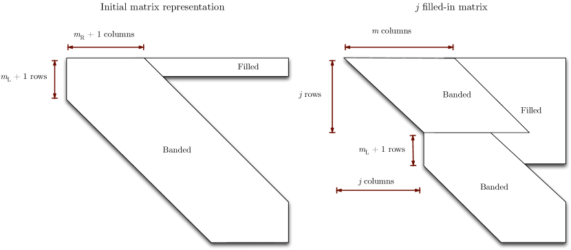
Fig. 7: Structure of operators during QR factorization. Left: Depicts the structure of the original differential operator. Right: Depicts a $j$ filled-in matrix obtained after upper triangularizing the first $j$ columns.

We will solve $Ax=b$ by computing a $QR$ factorization using Given’s rotations. However, the resulting upper triangular part will be dense because of fill-in caused by the boundary rows. We will show that these dense rows can still be represented sparsely, and that the resulting upper triangular matrix can be solved in $\mathcal{O}(m^{2}n)$ operations.

Remark 5.13.

Alternatively, the $A=QRP^{*}$ decomposition can be constructed in $\mathcal{O}(m^{2}n)$ operations by apply Given’s rotations to the left and the right, which prevents the boundary row(s) causing fill-in [8]. However, with this decomposition it is unclear whether the optimal truncation $n_{\rm opt}$ can be determined in ${\cal O}(n_{\rm opt})$ operations.

5.1 QR factorization for filled-in matrices

Represent the matrix $A$ after the $j$th stage of the QR decomposition, where the $j$th column has been completely reduced, by $B$. We claim that $B$ has the form of a $j$ filled-in matrix.

Definition 5.14.

$B$ is a $j$ filled-in matrix if, for $k=1,\ldots,j$, the $k$th row of $B$ has the form

$${\bf e}_{k}^{\top}B=\Biggl{(} \overbrace{0,\ldots,0}^{k-1\hbox{ times}},\overbrace{B_{k,k},\dots,B_{k,k+m-1}}^{\hbox{banded terms}},\overbrace{{\bf b}_{k}^{\top}{\cal B}_{1:K,k+m:n}}^{\hbox{fill-in terms}}\Biggr{)},$$ (27)

where ${\bf b}_{k}\in{\mathbb{C}}^{K}$. Furthermore, every row $k=j+1,\ldots,j+m_{\rm L}+1$ has the form

$${\bf e}_{k}^{\top}B=\Biggl{(}\overbrace{0,\ldots,0}^{j\hbox{ times}},\overbrace{B_{k,j+1},\dots,B_{k,k+m_{\rm R}}}^{\hbox{banded terms}},\overbrace{{\bf b}_{k}^{\top}{\cal B}_{1:K,k+m_{\rm R}+1:n}}^{\hbox{fill-in terms}}\Biggr{)}.$$

The remaining rows have the form

$${\bf e}_{k}^{\top}B=\Biggl{(}\overbrace{0,\ldots,0}^{k-m_{\rm L}-1\hbox{ times}},\overbrace{B_{k,k-m_{\rm L}},\dots,B_{k,k+m_{\rm R}}}^{\hbox{banded terms}},\overbrace{0,\ldots,0}^{\hbox{$n-k-m_{\rm R}$ times}}\Biggr{)}.$$ (28)

See Figure 7 for a depiction of a $j$ filled-in matrix. Essentially, it is a banded matrix where the top-right part can be filled with linear combinations of the boundary rows. Note that each row of a filled-in matrix takes at most $m+K$ entries to represent, a bound which is independent of $j$. Since the QR factorization only applies Given’s rotations on the left (i.e. linear combinations of rows), and the initial matrix is a $0$ filled-in matrix, the elimination results in $j$ filled-in matrices. This means that throughout the elimination, the matrix can be represented with $\mathcal{O}(mn)$ storage.

In section 5.3, we perform QR factorization adaptively on the operator. This is successful because the representation as a $j$ filled-in matrix is independent of the number of columns, and the rows below the $(j+m_{\rm L})$th are unchanged from the original operator, hence can be added during the factorization.

5.2 Back substitution for filled-in matrices

After we have performed $n$ stages of Given’s rotations, the first $n$ rows are of the form (27) and hence are upper triangular. Thus, we can now perform back substitution, by truncating the right-hand side. The last $m$ rows consist only of banded terms, and standard back substitution is used to calculate $u_{n-m+1},\ldots,u_{n}$. We then note that the $k$th row imposes the condition

$$B_{k,k}u_{k}=c_{k}-\sum_{s=1}^{m}B_{k,k+s}u_{k+s}-{\bf b}_{k}^{\top}\sum_{s=k+m+1}^{n}{\cal B}_{1:K,s}u_{s}$$

on the solution. We can thus obtain an ${\cal O}(mn)$ back substitution algorithm by the following:

Algorithm 1 Back substitution for filled-in matrices

$\mathbf{p}_{n-m}=\mathbf{0}$             (i.e., a vector of $K$ zeros)

for $k=n-m-1\to 1$ do

     $\mathbf{p}_{k}={u_{k+m+1}\mathcal{B}}_{1:K,k+m+1}+\mathbf{p}_{k+1}$

     $u_{k}=\frac{1}{B_{k,k}}\left(c_{k}-\sum_{s=1}^{m}B_{k,k+s}u_{k+s}-{\mathbf{b}}_{k}^{\top}{\mathbf{p}}_{k}\right)$

end for

This is mathematically equivalent to standard back substitution. However, the reduced number of operations decreases the accumulation of round-off error.

5.3 Optimal truncation

One does not know apriori how many coefficients $n_{\rm opt}$ are required to resolve the solution to relative machine precision. A straightforward algorithm for finding $n_{\rm opt}$ is to continually double the discretization size until the difference in the computed coefficients is below a given threshold, which will result in an ${\cal O}(n_{\rm opt}\log{n_{\rm opt}})$ algorithm. We will present an alternative approach that achieves the optimal ${\cal O}(n_{\rm opt})$ complexity.

For the simple equation

$$u^{\prime}+u=f\qquad\hbox{and}\qquad u(1)=c,$$

the truncation of the operator is tridiagonal with a single dense boundary row. This is equivalent to an inhomogeneous three-term recurrence boundary value problem. The problem of adaptively truncating such recurrence relationships is solvable by (F. W. J.) Olver’s algorithm [33]. The central idea is to apply row reduction (without pivoting) adaptively. The row-reduction applied to the right-hand side, when combined with a concurrent adaptive computation of the homogeneous solutions to the recurrence relationship, allowed an explicit bound for the relative error. An alternative (and simpler) bound for the absolute error was obtained in examples. The case of dense boundary rows, with an application to the Clenshaw method [9] as motivation, was also considered. Adaptation of the algorithm to higher order difference equations was developed by Lozier [30].

We adapt this approach to our case by incorporating it into the QR factorization of subsection 5.1. By using QR factorization in place of Gaussian elimination, we avoid potential numerical stability issues of the original Olver’s algorithm in the low order coefficients. The key observation is that the boundary terms ${\cal B}$ and the rows of the form (28) can be evaluated lazily, with bounded computational cost per entry. Thus the truncation parameter $n$ is not involved in the proposed QR factorization algorithm (only in the back substitution), hence the optimal truncation $n_{\rm opt}$ can be found adaptively.

Represent the Given’s rotations that reduces the first $n$ columns of ${\cal A}$ by the orthonormal operator $Q_{n}\in{\mathbb{C}}^{(n+m_{\rm L})\times(n+m_{\rm L})}$, so that

$$\begin{pmatrix}{Q}_{n}^{\star}\cr&I\end{pmatrix}{\cal A}=\begin{pmatrix}R_{n}&{\cal F}\cr&{\cal W}\end{pmatrix}$$

where $R_{n}\in{\mathbb{C}}^{n\times n}$ is upper triangular. Our right-hand side is

$$\begin{pmatrix}{Q}_{n}^{\star}\cr&I\end{pmatrix}\begin{pmatrix}{\bf c}\\ {\cal S}_{N-1}\cdots{\cal S}_{0}\mathbf{f}\end{pmatrix}=\begin{pmatrix}\mathbf{r}_{1:n}\\ \mathbf{r}_{n+1:n+m_{\rm L}}\\ \mathbf{0}\end{pmatrix}$$

where we use the fact that $\mathbf{f}$ has only finite number of nonzero entries and assume that $n+m_{\rm L}$ is greater than the number of nonzero entries. Thus our numerical approximation ${\mathbf{u}}_{n}=R_{n}^{-1}\mathbf{r}_{1:n}$ has the forward error:

$$\begin{pmatrix}{Q}_{n}^{\star}\cr&I\end{pmatrix}{\cal A}\begin{pmatrix}{\mathbf{u}}_{n}\\ {\bf 0}\\ {\bf 0}\end{pmatrix}-\begin{pmatrix}\mathbf{r}_{1:n}\\ \mathbf{r}_{n+1:n+m_{\rm L}}\\ {\bf 0}\end{pmatrix}=\begin{pmatrix}R_{n}{\mathbf{u}}_{n}\\ {\bf 0}\\ {\bf 0}\end{pmatrix}-\begin{pmatrix}\mathbf{r}_{1:n}\\ \mathbf{r}_{n+1:n+m_{\rm L}}\\ {\bf 0}\end{pmatrix}=\begin{pmatrix}{\bf 0}\\ \mathbf{r}_{n+1:n+m_{\rm L}}\\ {\bf 0}\end{pmatrix}.$$

Since we calculate $\mathbf{r}_{n+1:n+m_{\rm L}}$ during the algorithm, we know the forward error exactly. Having a bound on $\|{\cal A}^{-1}\|$ allows us to bound the backward error; i.e., $\|{\mathbf{u}}-{\cal P}_{n}^{\top}{\mathbf{u}}_{n}\|$. This can be improved further by adapting the procedure of [33, 30], which in a sense calculates an alternative bound based on the homogeneous solutions of the difference equation as part of the algorithm.

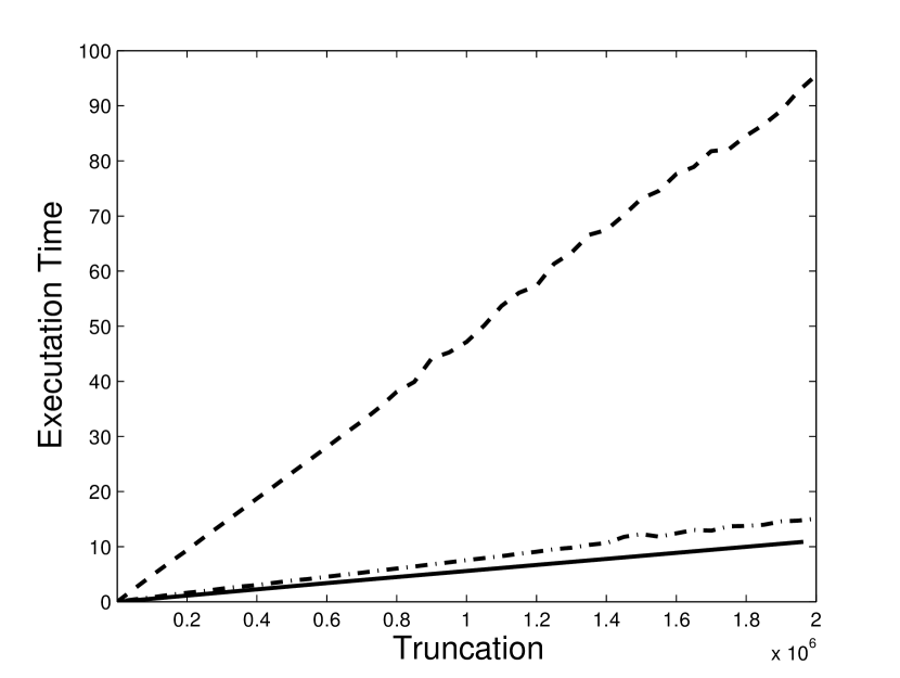
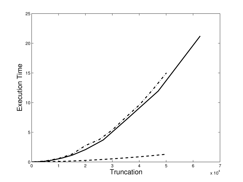
Fig. 8: Time versus optimal truncation, showing linear computational cost for the C++ implementation (left) and the Matlab implementation (right). Examples are (25) (solid), (29) (dot-dashed) and (30) (dashed).

In Figure 8, we apply the adaptive QR decomposition to solve the Airy equation of example (25) with $\epsilon=1,10^{-1},10^{-2},\ldots,10^{-13}$, as well as

$$u^{\prime\prime}+(7+2x+6x^{2})u =\sum_{k=0}^{\nu}T_{k}(x)\hbox{ for }u(-1)=1,u(1)=1,$$ (29)

$$u^{\prime\prime}+\cos xu =\sum_{k=0}^{\nu}T_{k}(x)\hbox{ for }u(-1)=1,u(1)=1$$ (30)

for increasing values of $\nu$, up to 2 million. In the last example, we replace $\cos x$ with its 13 point Chebyshev interpolating polynomial. We plot the number of seconds the calculation takes versus the adaptively calculated optimal truncation $n_{\rm opt}$. This demonstrates the ${\cal O}(n_{\rm opt})$ complexity of the algorithm, and the fact that the algorithm easily scales to more than a million unknowns. It also shows that, while ${\cal O}(n_{\rm opt})$ complexity is maintained, the computational cost does increase with the bandwidth of the variable coefficient. In the Airy example (25), the time taken for $\epsilon=10^{-13}$ is less than 11 seconds, with the $n_{\rm opt}$ calculated to be approximately 2 million. For example (30), a calculation resulting in $n_{\rm opt}$ being 2 million increases the timing to 95 seconds.

On the right of Figure 8 we plot the timing of Matlab’s built-in sparse LU solver applied to the truncated equation, with $n=n_{\rm opt}$ pre-specified. Even without the added difficulty of calculating $n_{\rm opt}$, the computational cost grows faster than ${\cal O}(n)$, prohibiting its usefulness for extremely large $n$.

Remark 5.15.

We calculated Figure 8 using C++. There is a great deal of room for optimizing the implementation, as we do not use GPU, parallel or vector processing units.

5.4 Linear algebra stability in higher order norms

We first remark that, if ${\cal B}$ is a bounded operator from $\ell^{2}_{1}\rightarrow\ell^{2}_{0}$, such as Dirichlet boundary conditions, then the results of section 4 prove that the preconditioned linear system has bounded $2$-norm condition number as $n\rightarrow\infty$. Because the $QR$ decomposition is computed using Givens rotations, which are stable in $\ell^{2}_{0}$ [27], as is backward substitution, we see that the linear algebra scheme applied to the preconditioned operator is stable, and has ${\cal O}(m^{2}n)$ complexity.

The results of section 4 also show convergence and well-conditioning in high order norms. One would expect numerical round-off in $QR$ decomposition to destroy this convergence property. However, in practice, this is not the case. In Figure 9, we solve the standard Airy equation as a two point boundary value problem:

$$u^{\prime\prime}-xu=0,\quad u(-1)={\text{Ai}}(-1)\hbox{ and }u(1)={\text{Ai}}(1).$$

We witness convergence in higher order norms as well. In other words, the computed solution has a fast decaying tail, and all of the absolute error is in the low order coefficients.

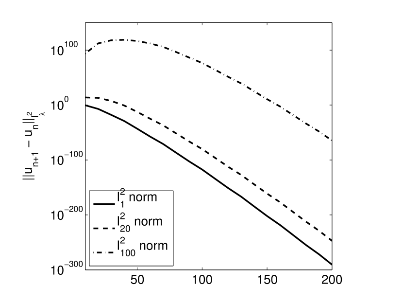
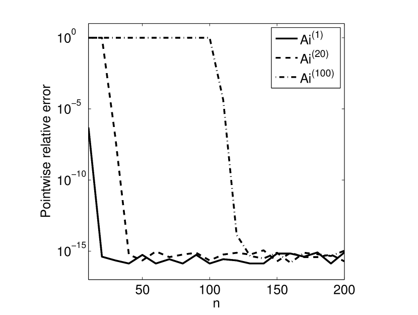
Fig. 9: Left: The Cauchy error of the solution coefficients measured in the: (solid) $\ell_{1}^{2}$-norm, (dashed) $\ell_{20}^{2}$-norm, (dot-dashed) $\ell_{100}^{2}$-norm. Right: The relative error in derivatives of the solution at $x=-\frac{1}{2}$ for the $1$st (solid), $20$th (dashed), $100$th (dot-dashed) derivative. This plot shows that for sufficiently large discretisations very high derivatives of the solution can be resolved.

Convergence in higher order norms implies convergence of derivatives, and this is verified by differentiating the computed solution by applying ${\cal S}_{0}^{-1}{\cal D}_{1}$ repeatedly. (We note that the banded, upper triangular nature of ${\cal S}_{0}$ means that its inverse applied to a vector is computable in ${\cal O}(n)$ operations; after all, this corresponds to differentiating without converting bases which can be done in $\mathcal{O}(n)$ operations [32].) We compare the computed derivatives with the true derivatives of the Airy function ${\text{Ai}}^{(p)}$ at a single point, $x=-1/2$, and witness convergence for $p=1,5$ and $20$.

We note that the stability of the $QR$ algorithm in higher order norms appears to follow from $Q$ being almost banded: it is banded along the superdiagonal, and decays exponentially along the subdiagonals. In the case where the boundary conditions are such that $A$ itself is banded, exponential decay in $Q=AR^{-1}$ follows since $R^{-1}$ has exponentially decay, due to $R$ being banded and well-conditioned [13].

Since $\ell^{2}_{\lambda}$ is a Hilbert space, Givens rotations can be constructed with the relevant inner product, resulting in orthogonal operations (i.e., with condition number one) in $\ell^{2}_{\lambda}$. The stability of such an algorithm in $\ell^{2}_{\lambda}$ follows immediately. With this modification, we have an ${\cal O}(m^{2}n)$ stable algorithm which is guaranteed to converge in higher order norms.

Remark 5.16.

While we have discussed the convergence in higher order norms with Dirichlet boundary conditions, the exact same logic applies to the convergence and stability observed with higher order boundary conditions, such as Neumann conditions.

6 Future work

We have designed a spectral method that achieves ${\cal O}(n)$ computational cost, stability and generality for solving linear ODEs. We determined the optimal truncation adaptively using the QR factorization. We believe that the ideas introduced in this paper will serve as a basis for future spectral methods.

An exciting generalization of this work will be to higher dimensions, where the density of matrices has inhibited the usefulness of spectral methods. A similar approach, based on boundary recombination, was used in [41] for the Helmholtz equation. Adapting our method to rectangular domains, using tensor products of ultraspherical polynomials, results in a tensor product of almost banded matrices. Constructing an adaptive QR decomposition to such matrices will be crucial for achieving competitive computational costs, and for optimally choosing the number of unknowns needed in each dimension.

Using the theory of [40], there are potentially generalization of ultraspherical polynomials to deltoid domains. What is less clear is how the results would be generalizable to other domains, such as the the triangle.

For problems with boundary layers, or localized oscillatory behaviour, it can be more efficient to subdivide the unit interval, in order to minimize the total number of unknowns. This will be of fundamental importance for PDEs, where solutions typically have singularities at corners. In the 1D case, it is straightforward to incorporate subdivision by representing the operators as block matrices, with additional boundary rows to impose continuity. Whether the adaptive QR decomposition can be easily generalized to such matrices is less clear.

Finally, an extension of this work is to nonlinear differential equations, of the form

$${\cal B}u=\mathbf{0}\qquad\hbox{and}\qquad{\cal L}u+g(u)=f.$$

Our approach can be incorporated into an infinite-dimensional Newton iteration, á la [2, 18]. The Newton iteration takes the form

$$u_{k+1}=u_{k}+\begin{pmatrix}{\cal B}\\ {\cal L}+g^{\prime}(u_{k})\end{pmatrix}^{-1}\begin{pmatrix}\mathbf{0}\\ {\cal L}u_{k}+g(u_{k})-f\end{pmatrix}.$$

Since the linear operator that is inverted involves the solution itself, the bandedness of multiplication is lost, at least when naïvely implemented. It may be possible to overcome this difficulty by using the fact that the derivative for Newton iteration need not be accurate to machine precision. Moreover, the decay in the coefficients of the operator can combine with decay in the solution, hence the entries of the operator can be truncated more aggressively while maintaining accuracy. However, even with a dense representation of the operator, the stability of the resulting algorithm is preserved in initial numerical experiments.

References

- [1] G. Baszenski and M. Tasche, Fast polynomial multiplication and convolutions related to the discrete cosine transform, Lin. Alg. Appl., 252 (1997), pp. 1–25.
- [2] A. Birkisson and T. A. Driscoll, Automatic Fréchet differentiation for the numerical solution of boundary-value problems, ACM Trans. Math. Softw., to appear.
- [3] C. M. Bender and S. A. Orszag, Advanced Mathematical Methods for Scientists and Engineers, McGraw–Hill, (1978).
- [4] J. P. Boyd, Chebyshev and Fourier Spectral Methods, Dover Publications, (2001).
- [5] C. Canuto and A. Quarteroni, Preconditioned minimal residual methods for Chebyshev spectral calculations, Jour. Comp. Phys., 60 (1985), pp. 315–337.
- [6] C. Canuto, Spectral Methods: Fundamentals in Single Domains, Springer, (2006).
- [7] L. Carlitz, The product of two ultraspherical polynomials, Proc. Glasgow Math. Assoc., 5 (1961), pp. 76–79.
- [8] S. Chandrasekaran and M. Gu, Fast and atable algorithms for banded plus semiseparable systems of linear equations, SIAM Jour. Mat. Anal. App., 25 (2003), pp. 373–384.
- [9] C. W. Clenshaw, The numerical solution of linear differential equations in Chebyshev series, Proc. Camb. Philos. Soc., 53 (1957), pp. 134–149.
- [10] C. W. Clenshaw and A. R. Curtis, A method for numerical integration on an automatic computer, Numer. Math., 2 (1960), pp. 197–205.
- [11] E. A. Coutsias, T. Hagstrom and D. Torres, An efficient spectral method for ordinary differential equations with rational function coefficients, Math. Comp., 65 (1996), pp. 611–635.
- [12] P. J. Davis Interpolation and Approximation, Dover, (1975).
- [13] S. Demko, W. F. Moss and P. W. Smith, Decay rates for inverse of band matrices, Math. Comp., 43 (1984), pp. 491–499.
- [14] M. Deville and E. Mund, Chebyshev pseudospectral solution of second-order elliptic equations with finite element preconditioning, Jour. Comp. Phys., 60 (1985), pp. 315–337.
- [15] E. H. Doha and W. M. Abd-Elhameed, Efficient spectral-Galerkin algorithms for the direct solutions of second-order equations using ultraspherical polynomials, SIAM J. Sci. Comp., 24 (2002), pp. 548–571.
- [16] E. H. Doha, On the construction of recurrence relations for the expansion and connection coefficients in series of Jacobi polynomials, J. Phys. A: Math. Gen., 37 (2004), pp. 657–675.
- [17] E. H. Doha and W. M. Abd-Elhameed, Efficient spectral ultraspherical-dual-Petrov–Galerkin algorithms for the direct solution of th-order linear differential equations, Math. Comp. Simul., 79 (2009), pp. 3221–3242.
- [18] T. A. Driscoll, F. Bornemann and L. N. Trefethen, The chebop system for automatic solution of differential equations, BIT Numer. Math., 48 (2008), pp. 701–723.
- [19] T. A. Driscoll, Automatic spectral collocation for integral, integro-differential, and integrally reformulated differential equations, Jour. Comp. Phys., 229, 17 (2010), pp. 5980–5998.
- [20] E. M. E. Elbarbary, Integration preconditioning matrix for ultraspherical pseudospectral operators, SIAM J. Sci. Comput., 48 (2006), pp. 701–723.
- [21] B. Fornberg, A Practical Guide to Pseudospectral Methods, Cambridge University Press, (1998).
- [22] L. Fox, Chebyshev methods for ordinary differential equations, The Computer Journal, 4 (1962), pp. 318–331.
- [23] D. Gottlieb and S. A. Orzag, Numerical Analysis of Spectral Methods: Theory and Applications, SIAM, (1977).
- [24] L. Greengard, Spectral integration and two-point boundary value problems, SIAM J. Numer. Anal., 4 (1991), pp. 1071–1080.
- [25] A. C. Hansen, Infinite dimensional numerical linear algebra; theory and applications, Proc. R. Soc. Lond. Ser. A, 466 (2008) pp. 3539–3559
- [26] J. S. Hesthaven Integration Preconditioning of Pseudospectral Operators. I. Basic Linear Operators, SIAM Jour. Numer. Anal., 35 (1998) pp. 1571–1593.
- [27] N. J. Higham, Accuracy and Stability of Numerical Algorithms, SIAM, (2002).
- [28] C. Lanczos Trigonometric interpolation of empirical and analytical functions, J. Math. Phys., 17 (1938) pp. 123–199.
- [29] J.-Y. Lee and L. Greengard A fast adaptive numerical method for stiff two-point boundary value problems, SIAM Jour. Sci. Comp., 18 (1997) pp. 403–429.
- [30] D. W. Lozier Numerical Solution of Linear Difference Equations, NBSIR Technical Report 80-1976, National Bureau of Standards, (1980).
- [31] H. Ma and W. Sun, A Legendre–Petrov–Galerkin and Chebyshev collocation method for third-order differential equations, SIAM J. Numer. Anal., 38 (2000), pp. 1425–1438.
- [32] J. C. Mason and D. C. Handscomb, Chebyshev Polynomials, Chapman & Hall/CRC, (2003).
- [33] F. W. J. Olver, Numerical solution of second-order linear difference equations, J. Res. Nat. Bur. Standards Sect. B, 71 (1967), pp. 111–129
- [34] F. W. J. Olver, D. W. Lozier, R. F. Boisvert and C. W. Clark, NIST Handbook of Mathematical Functions, Cambridge University Press, (2010).
- [35] S. Olver and A. Townsend, https://github.com/dlfivefifty/Ultraspherical.
- [36] S. A. Orszag, Spectral methods for problems in complex geometries, Jour. Comp. Phys., 50 (1971), pp. 689–703.
- [37] S. A. Orszag, Accurate solution of the Orr–Sommerfeld stability equation, J. Fluid Mech., 37 (1980), pp. 70–92.
- [38] E. L. Ortiz, The tau method, SIAM J. Numer. Anal., 6 (1969), pp. 480–492.
- [39] P. D. Ritger and N. J. Rose, Differential Equations with Applications, Dover Publications, (2000).
- [40] B. N. Ryland and H. Z. Munthe–Kaas, On multivariate Chebyshev polynomials and spectral approximations on triangles, in: Spectral and High Order Methods for Partial Differential Equations, Springer Berlin Heidelberg, (2011), pp. 19–41.
- [41] J. Shen, Efficient spectral-Galerkin method II. Direct solvers of second- and fourth-order equations using Chebyshev polynomials, SIAM J. Sci. Comput., 16 (1995), pp. 74–87.
- [42] J. Shen, A new dual-Petrov–Galerkin method for third and higher odd-order differential equations: application to the KdV equation, SIAM J. Numer. Anal., 41 (2004), pp. 1595–1619.
- [43] J. Shen and L. L. Wang, Legendre and Chebyshev dual-Petrov–Galerkin methods for Hyperbolic equations, Comput. Methods Appl. Mech. Engrg., 196 (2007), pp. 3785–3797.
- [44] J. Shen, T. Tang and L. L. Wang, Spectral Methods: Algorithms, Analysis and Applications, Springer, (2009).
- [45] L. N. Trefethen, Spectral Methods in Matlab, SIAM, (2000).
- [46] L. N. Trefethen et al., Chebfun Version 4.2, The Chebfun Development Team, (2011), http://www.maths.ox.ac.uk/chebfun/.
- [47] D. Viswanath, Spectral integration of linear boundary value problems, (2012), preprint.
- [48] J. Waldvogel, Fast construction of the Fejér and Clenshaw–Curtis quadrature rules, BIT Numer. Math., 46 (2006), pp. 195–202.
- [49] J. A. Weideman and S. C. Reddy, A Matlab differentiation matrix suite, ACM Transactions on Mathematical Software, 26 (2000), pp. 465–519.
- [50] A. Zebib, A Chebyshev method for the solution of boundary value problems, Jour. Comp. Phys., 53 (1984), pp. 443–455.