Anomalous growth of thermoelectric power in gapped graphene

Abstract

There exist experiments indicating that at certain conditions, such as an appropriate substrate, a gap of the order of 10 meV can be opened at the Dirac points of a quasiparticle spectrum of graphene. We demonstrate that the opening of such a gap can result in the appearance of a fingerprint bump of the Seebeck signal when the chemical potential approaches the gap edge. The magnitude of the bump can be up to one order higher than the already large value of the thermopower occurring in graphene. Such a giant effect, accompanied by the nonmonotonous dependence on the chemical potential, is related to the emergence of a new channel of quasiparticle scattering from impurities with the relaxation time strongly dependent on the energy. We analyze the behavior of conductivity and thermopower in such a system, accounting for quasiparticle scattering from impurities with the model potential in a self-consistent scheme. Reproducing the existing results for the case of gapless graphene, we demonstrate a failure of the simple Mott formula in the case under consideration.

Control of heat flows and minimization of heat losses is an important aspect of designing modern nanoelectronic devices, in particular those based on graphene Geim2009Science . Experiments indicate Grosse2011NatureNano that the thermoelectric effect in graphene accounts for up to one-third of the contact temperature changes and thus it can play a significant role in cooling down of such systems. The measured thermopower $S$ reaches the value $k_{B}/e\sim 100\mu V/K$ at room temperatures, where $k_{B}$ is the Boltzmann constant and $-e<0$ is the electron charge. This and other experimental results Wei2009PRL ; Zuev2009PRL ; Checkelsky2009PRB ; Wang2011PRB on thermoelectric transport in graphene were understood theoretically, mostly basing them on a simple Mott relation between thermopower and the logarithmic derivative of the electrical conductivity $\sigma(\mu,T)$,

$$S(\mu,T)=-\frac{\pi^{2}}{3e}T\frac{d}{d\mu}[\ln\sigma(\mu,T=0)],$$ (1)

where $\mu$ is the chemical potential and $T$ is the temperature (we set $k_{B}=1$) xx . However, the cited experiments show that the Mott formula (1) fails when $\mu$ approaches the vicinity of the Dirac point at high temperatures, especially in high-mobility graphene Wang2011PRB . The available theoretical analysis Lofwander2007PRB ; Hwang2009PRB ; Ugarte2011PRB shows that the failure of Eq. (1) can be attributed to breaking of the conditions of its applicability, which read as $T\ll|\mu|$ and/or $T\ll\gamma$ [here $\gamma$ is the characteristic energy scale on which the conductivity $\sigma(\mu,T=0)$ varies around the Fermi level].

The purpose of the present paper is to show that the already large value of the thermopower occurring in graphene can be further increased up to one order of magnitude by opening in different ways (see, e.g., Refs. Gusynin2007IJMPB, ; Vozmediano2011, ) a gap $\Delta$ in its quasiparticle spectrum. We will show that such an opening is accompanied by the emergence of a new channel of quasiparticle scattering with the relaxation time strongly dependent on energy, and it results in the appearance of a giant bump in thermopower when chemical potential approaches the gap edge. The situation here turns out to be very similar to the well known anomaly of thermopower close to the electronic topological transition (see Refs. Varlamov1989AP, ; Blanter1994PR, for a review) related to the scattering of electrons from all of the extended periphery of the Fermi surface to the “trap,” presented by the small new void or narrow “neck” of the latter.

It is worth mentioning that some experimental findings Zhou2007NatMat ; Li2009PRL indicate that, indeed, a gap in the graphene quasiparticle spectrum opens at the Dirac point, and probably it can be attributed to the effect of the substrate. Yet, this issue still remains an open problem of the physics of graphene Gusynin2007IJMPB ; Vozmediano2011 . This is why, in principle, one can apply the results obtained below and use thermopower measurements as a sensitive probe of the gap opening in the graphene spectrum.

The Hamiltonian for graphene can be written down in the momentum representation as

$$\widehat{H}=\sum_{\sigma}\int_{BZ}\frac{d^{2}p}{(2\pi)^{2}}\Upsilon_{\sigma}^{\dagger}(\mathbf{p})[\widehat{\mathcal{H}}(\mathbf{p})-\mu\widehat{\tau}_{0}]\Upsilon_{\sigma}(\mathbf{p}),$$ (2)

where

$$\widehat{\mathcal{H}}(\mathbf{p})=\widehat{\tau}_{+}\phi\left(\mathbf{p}\right)+\widehat{\tau}_{-}\phi^{\ast}\left(\mathbf{p}\right)+\Delta\widehat{\tau}_{3},$$

$\widehat{\tau}_{0}$, $\widehat{\tau}_{3}$, and $\widehat{\tau}_{\pm}=(\widehat{\tau}_{1}\pm i\widehat{\tau}_{2})/2$ are Pauli matrices acting in the sublattice space on the spinors, $\Upsilon_{\sigma}(\mathbf{p})$ and $\Upsilon_{\sigma}^{\dagger}(\mathbf{p})=\left(a_{\sigma}^{\dagger}(\mathbf{p}),b_{\sigma}^{\dagger}(\mathbf{p})\right)$, with the creation (annihilation) operators of electrons $a_{\sigma}^{\dagger}(\mathbf{p})$, $b_{\sigma}^{\dagger}(\mathbf{p})$ ($a_{\sigma}(\mathbf{p})$, $b_{\sigma}(\mathbf{p})$) corresponding to $A$ and $B$ sublattices, respectively, and spin subscript $\sigma$. The full form of the complex function $\phi(\mathbf{p})$ is provided, for example, in Ref. Gusynin2007IJMPB, and in present consideration it is important only that near two independent $\mathbf{K}$ points the dispersion $\xi\equiv|\phi(\mathbf{p})|=\hbar v_{F}|\mathbf{p}|$, where $v_{F}$ is the Fermi velocity and the the wave vector $\mathbf{p}$ is measured from the corresponding $\mathbf{K}$ point. In the result of diagonalization of the operator (2) one finds that the presence of the gap $\Delta$ in it breaks the equivalence between $A$ and $B$ sublattices, and the spectrum of the quasiparticle excitations close to the $\mathbf{K}$ points takes the form $E\left(\mathbf{p}\right)=\pm\sqrt{\hbar^{2}v_{F}^{2}\mathbf{p}^{2}+\Delta^{2}}-\mu$.

We will account for the quasiparticle scattering from impurities in the framework of the Abrikosov-Gorkov scheme, writing the self-consistent equation for self-energy in the matrix form

$$\widehat{\Sigma}(\mathbf{p},\varepsilon_{n})=n_{i}\int_{BZ}\frac{d^{2}q}{(2\pi)^{2}}\widehat{V}(\mathbf{q})\widehat{G}(\mathbf{p-q},\varepsilon_{n})\widehat{V}(\mathbf{q}),$$ (3)

with $n_{i}$ as concentration of impurities and $\varepsilon_{n}=\pi T(2n+1)$, the full inverse Green’s function (GF)

$$\widehat{G}^{-1}(\mathbf{p},\varepsilon_{n})=\widehat{G}_{0}^{-1}(\mathbf{p},\varepsilon_{n})-\widehat{\Sigma}(\mathbf{p},\varepsilon_{n}),$$ (4)

and the free inverse Green’s function

$$\widehat{G}_{0}^{-1}(\mathbf{p},\varepsilon_{n})=(i\varepsilon_{n}+\mu)\widehat{\tau}_{0}-\widehat{\mathcal{H}}(\mathbf{p}).$$ (5)

The sublattices $A$ and $B$ are shifted by a distance of the order of lattice constant $a$, hence their images in inverse space are separated by momenta of the order of $\hbar/a.$ Hence, for the relatively long-range potential $\widehat{V}(\mathbf{q})$ in Eq. (3) one can ignore the quasi-particle scattering between the inequivalent valleys. At the same time we will assume $\widehat{V}(\mathbf{q})$ as momentum independent for the intra-valley scattering, i.e.

$$\widehat{V}(\mathbf{q})=\widehat{\tau}_{0}\left\{\begin{array}[]{cc}u(\mathbf{0}),&|q|\lesssim\frac{\max\left\{|\mu|,\Delta\right\}}{\hbar v_{F}}\\ 0,&\frac{\max\left\{|\mu|,\Delta\right\}}{\hbar v_{F}}\ll|q|\lesssim\frac{\hbar}{a}.\end{array}\right.$$ (6)

The next step in the solution of Eq. (3) is the decomposition of the self-energy over Pauli matrices $\widehat{\Sigma}(\mathbf{p},\varepsilon_{n})=\sum_{i=0}^{3}\sigma_{i}(\mathbf{p},\varepsilon_{n})\widehat{\tau}_{i}$. One can see that by ignoring the self-consistence procedure in Eq. (3) with potential (6) (which does not mix valleys), one obtains $\widehat{\Sigma}^{\left(0\right)}(\mathbf{p},\varepsilon_{n})$ in the diagonal form. It is possible to show that the off-diagonal components appear in the order $n_{i}^{2}$ only, i.e. $\sigma_{1}^{R}(\mathbf{p},\varepsilon_{n})$ and $\sigma_{2}^{R}(\mathbf{p},\varepsilon_{n})$ terms can be omitted. Finally, the momentum dependence of $\widehat{\Sigma}(\mathbf{p},\varepsilon_{n})$ can be also ignored in view of the constancy of potential (6) in the domain of each valley and taking into account that the main contribution to $\widehat{\Sigma}$ appears from the relatively large momenta $|\mathbf{q}|\sim\max\left\{|\mu|,\Delta\right\}/\hbar v_{F}$. This latter fact justifies our use of the Abrikosov-Gorkov technique for averaging of the quasiparticle scattering over impurity positions. As a result, after the analytical continuation $i\varepsilon_{n}\rightarrow\varepsilon$, the matrix Eq. (3) reduces to the system of two equations footnote

$$\begin{split}&\left\{\begin{array}[]{c}\sigma_{0}^{R}(\varepsilon)\\ \sigma_{3}^{R}(\varepsilon)\\ \end{array}\right\}=\frac{4\hbar}{\pi\tau_{0}|\mu|}\left\{\begin{array}[]{c}\varepsilon+\mu-\sigma_{0}^{R}(\varepsilon)\\ \Delta+\sigma_{3}^{R}(\varepsilon)\\ \end{array}\right\}\\ &\times\int_{0}^{W}\frac{\xi d\xi}{\left[\varepsilon+\mu-\sigma_{0}^{R}(\varepsilon)\right]^{2}-\xi^{2}-[\Delta+\sigma_{3}^{R}(\varepsilon)]^{2}},\end{split}$$ (7)

where we introduce the “relaxation time scale”Peres2007PRB

$$\frac{1}{\tau_{0}}=\frac{n_{i}|u(\mathbf{0})|^{2}|\mu|}{4\hbar^{3}v_{F}^{2}}.$$ (8)

The real parts $\mbox{Re}\,\sigma_{0}^{R}$ and $\mbox{Re}\,\sigma_{3}^{R}$, which are logarithmically dependent on the high energy cutoff $W,$ can be included in the renormalized $\mu$ and $\Delta$, respectively. For the self-energy imaginary parts, which determine the quasiparticle relaxation rate, one finds

$$\begin{split}&\!\!\!\!\!\!\!\!\!\left\{\!\!\begin{array}[]{c}\mbox{Im}\,\sigma_{0}^{R}(\varepsilon)\\ \mbox{Im}\,\sigma_{3}^{R}(\varepsilon)\\ \end{array}\!\!\right\}=-\frac{2\theta\left[\left(\varepsilon+\mu\right)^{2}-\Delta^{2}\right]\mathrm{sgn}\!\left(\varepsilon+\mu\right)}{(\tau_{0}/\hbar)|\mu|}\left\{\!\!\begin{array}[]{c}\varepsilon+\mu\\ \Delta\\ \end{array}\!\!\right\}.\end{split}$$ (9)

One can note that the denominator of the full GF (4) can be approximated as:

$$\begin{split}&[\varepsilon+\mu-i\mbox{Im}\,\sigma_{0}^{R}(\varepsilon)]^{2}-\xi^{2}-[\Delta+i\mbox{Im}\,\sigma_{3}^{R}(\varepsilon)]^{2}\\ &\approx[\varepsilon+\mu+i\Gamma(\varepsilon)]^{2}-E^{2}(\mathbf{p}),\end{split}$$

so that the full inverse GF can now be written as $[\widehat{G}^{R}(\mathbf{p},\varepsilon+i0)]^{-1}\approx[\widehat{G}_{0}^{R}(\mathbf{p},\varepsilon)]^{-1}+i\widehat{\tau}_{0}\Gamma(\varepsilon)$. Here the energy-dependent scattering rate $\Gamma(\varepsilon)$, central for our consideration, explicitly appears:

$$\begin{split}\Gamma(\varepsilon)&=-\mbox{Im}\,\sigma_{0}^{R}(\varepsilon)-\frac{\Delta}{\varepsilon+\mu}\mbox{Im}\,\sigma_{3}^{R}(\varepsilon)\\ =&\Gamma_{0}\left[\frac{|\varepsilon+\mu|}{|\mu|}+\frac{\Delta^{2}}{|\varepsilon+\mu||\mu|}\right]\theta\left[\left(\varepsilon+\mu\right)^{2}-\Delta^{2}\right]\end{split}$$ (10)

with $\Gamma_{0}=2\hbar/\tau_{0}$. In the numerical results presented below we use the value $\Gamma_{0}=20\,\mbox{K}$ ignoring its dependence on the carrier concentration.

It follows from Eq. (10) that for $(\varepsilon+\mu)^{2}<\Delta^{2}$ the scattering is absent. Further consideration shows that in spite of the presence of $\Gamma(\varepsilon)$ in the denominators of Eq. (12), this fact does not result in divergence of the physical observables. Yet, one should keep in mind that some scattering processes beyond our model along with the next order corrections to the solution (9) can make the scattering rate finite below the gap edge. For our numerical work we took this into account by adding a small residual scattering rate $\gamma_{0}$ to $\Gamma(\varepsilon)$. In accordance to the theoretical analysis the final results turn out to be practically independent of the value $\gamma_{0}$.

Using the Kubo relations one can derive electric conductivity and thermoelectric coefficient in the explicit form

$$\left\{\begin{array}[]{c}\sigma\\ \beta\\ \end{array}\right\}=\frac{e^{2}}{\hbar}\int_{-\infty}^{\infty}\frac{d\varepsilon\mathcal{A}(\varepsilon,\Gamma(\varepsilon),\Delta)}{2T\cosh^{2}\frac{\varepsilon}{2T}}\left\{\begin{array}[]{c}1\\ \varepsilon/(eT)\\ \end{array}\right\},$$ (11)

where in the presence of $\Delta$ the function $\mathcal{A}$ is given by Gorbar2002PRB ; Gusynin2005PRB

$$\begin{split}\mathcal{A}(\varepsilon,\Gamma&(\varepsilon),\Delta)=\frac{1}{2\pi^{2}}\left[1+\frac{(\mu+\varepsilon)^{2}-\Delta^{2}+\Gamma^{2}(\varepsilon)}{2|\mu+\varepsilon|\Gamma(\varepsilon)}\right.\\ &\times\left.\left(\frac{\pi}{2}-\arctan\frac{\Delta^{2}+\Gamma^{2}(\varepsilon)-(\mu+\varepsilon)^{2}}{2|\mu+\varepsilon|\Gamma(\varepsilon)}\right)\right].\end{split}$$ (12)

For $\Delta=0$ Eq. (12) reduces to the commonly used expression (see, e.g., Refs. Lofwander2007PRB, ; Ugarte2011PRB, ). In this case, setting also $\Gamma(\varepsilon)=\Gamma_{0}=\mbox{const}$, one obtains for $|\mu|\gg T,\Gamma_{0}$ that $\sigma=e^{2}|\mu|/(2\pi\hbar\Gamma_{0})$ and $\beta=\pi eT\mathrm{sgn}\mu/(6\hbar\Gamma_{0})$, in agreement wit Ref. Gusynin2005PRB, . Then the value of the thermopower $S=-\beta/\sigma$ turns out to be the same as in the conventional metals, $S=-(\pi^{2}/3e)T/\mu$, and coincides with the result obtained directly from the Mott formula (1).

The dependences $\sigma(\mu)$, $\beta(\mu)$, and $S(\mu)$ are shown in the top, middle, and bottom panels of Fig. 1, respectively. The left side [Fig. 1 (a)] is for $T=1\,\mbox{K}$ and the right side [Fig. 1 (b)] is for $T=5\,\mbox{K}$. The dashed (red) curves in all panels correspond to the reference case $\Delta=0$, $\Gamma(\varepsilon)=\Gamma_{0}$, so that $\sigma(\mu)\varpropto|\mu|$ and $S(\mu)\varpropto 1/\mu$ for large $|\mu|$.

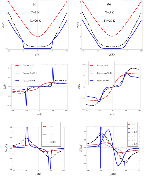
Figure 1: (Color online) Top panel: electrical conductivity $\sigma$ in units of the value $\sigma_{0}=2e^{2}/(\pi^{2}\hbar)$; middle panel: thermoelectric coefficient $\beta$ in units of the value $\beta_{0}=k_{B}e/\hbar$; bottom panel: thermopower $S$ in units of the value $k_{B}/e$ as functions of the chemical potential $\mu$. Left side: (a) for $T=1\,\mbox{K}$, and right side: (b) for $T=5K$. In all graphs three cases are shown: the dashed (red) curve is for the energy-independent scattering $\Gamma=\Gamma_{0}$ and $\Delta=0$, the dash-dotted (black) curve is for $\Gamma=\Gamma_{0}$ and $\Delta=50\,\mbox{K}$, and the solid (blue) curve is for energy-dependent $\Gamma(\varepsilon)$ and $\Delta=50\,\mbox{K}$. The solid curve in the bottom panel is multiplied by the factor $0.2$. The thin lines in the right bottom panel are obtained using the Mott formula.

The general expressions (11) and (12) also allow one to reproduce the gapped case with the energy-independent scattering $\Gamma(\varepsilon)=\Gamma_{0}$ Gorbar2002PRB ; Gusynin2005PRB . The corresponding reference dependences computed for $\Delta=50\,\mbox{K}$ are presented in all panels by the dash-dotted (black) curves.

Our main results obtained with the energy dependent $\Gamma(\varepsilon)$ given by Eq. (10) and $\Delta=50\,\mbox{K}$ are presented in all panels by the the solid (blue) curves.

The behavior of the conductivity $\sigma(\mu)$ is shown in the top panel of Fig. 1 (a) and (b). One can see that it drastically changes due to account for the energy dependence of $\Gamma(\varepsilon)$. Namely, a clear kink in the dependence $\sigma(\mu)$ appears at the gap edge, at $|\mu|=\Delta$, while below it, when $|\mu|<\Delta$, the value of $\sigma(\mu)$ is strongly suppressed as compared to the case $\Gamma(\varepsilon)=\Gamma_{0}$, $\Delta=\mbox{const}$. This kink is smeared out with the growth of temperature [Fig. 1 (b), $T=5\,\mbox{K}$].

Let us continue to the discussion of the Seebeck signal. In the gapless case with the constant scattering rate $\Gamma(\varepsilon)=\Gamma_{0}$ the signal monotonously changes with $\mu$ passing zero without any visible anomaly. The gap in the quasiparticle spectrum shows up as smoothed bumps at $|\mu|=\Delta$, which are rapidly smeared out by temperature (middle and bottom panels of Fig. 1).

The behavior of thermoelectric coefficient $\beta(\mu)$ and thermopower $S(\mu)$ in the case under consideration of gapped graphene with energy-dependent relaxation time is shown in the middle and bottom panels of Fig. 1 by the solid curves. Let us stress that the curves corresponding to $S(\mu)$ in the bottom panel are multiplied by the factor 0.2 to present them conveniently on the background of the previous cases. This means that the peaks of the Seebeck signal are at least five times higher than those ones obtained for $\Gamma(\varepsilon)=\mbox{const}$ case.

A strong enhancement of the Seebeck signal in the case when $\Gamma(\varepsilon)$ is energy dependent could be foreseen even basing on the Mott formula (1). However, this formula gives only a hint of the singular behavior of the Seebeck signal and cannot be used for any quantitative description. Indeed, the thin lines in the bottom panel of Fig. 1 (b) are computed using the zero-temperature electrical conductivity $\sigma(\mu,T=0)=(2e^{2}/\hbar)\mathcal{A}(0,\Gamma(0),\Delta)$ and the Mott formula (1), while the thick lines in the middle and bottom panels of Fig. 1 are plotted using the Kubo formulas (11) both for $\sigma$ and $\beta$. One finds that for the case of $\Delta=0$ and $\Gamma(\varepsilon)=\mbox{const}$ agreement between the Kubo and Mott formulas is very good. We checked that for $T=1\,\mbox{K}$ it becomes perfect, so that the lines for the Mott formula are not shown in the left bottom panel of Fig. 1. The right bottom panel shows that for the case of finite $\Delta$ and $\Gamma(\varepsilon)=\mbox{const}$ one can already see some discrepancies between the Kubo and Mott formulas, especially near $|\mu|=\Delta$. Finally, the Mott formula fails completely when the energy dependence of $\Gamma(\varepsilon)$ is taken into account.

Two more comments on the obtained bump of the Seebeck signal should be made. First, the shape of the bump depends on the presence of the $\sim\Delta^{2}$ term in Eq. (10) and thus accounting for the self-energy $\sigma_{3}(\varepsilon)$ is important for the qualitative theory. Second, our arguments are also directly applicable to gapped bilayer graphene, and indeed the computations done in Ref. Hao2010PRB, confirm this.

The applicability of the model potential (6) to the case under consideration deserves a more detailed discussion. It is worth stressing that we use it to solve the equation for self-energy with further fixation of $\Gamma_{0}=2\hbar\tau_{0}^{-1}\left(|\mu|=\Delta\right)=n_{i}|u(\mathbf{0})|^{2}|\Delta|/(2\hbar^{2}v_{F}^{2})$ [see Eq. (8)]. This procedure gives a consistent analytical treatment of the problem close to the gap edge $|\mu-\Delta|\ll\Delta,$ but it does not allow one to reproduce correctly the experimentally observed dependences of $\sigma$ and $S$ on the carrier concentration $n(\varpropto\mu^{2}\mathrm{sgn}\mu)$ beyond this region. In order to get a better agreement with the experiment in a wider interval of concentrations one could use the scattering potential $\widehat{V}(\mathbf{q})$ in the form of a long-range Coulomb one (see, for instance, Refs. Hwang2009PRB, ; Ugarte2011PRB, ; Peres2007PRB, ; Yan2009PRB, ). In such consideration one obtains that at large $n$ the scattering rate $\Gamma_{0}\varpropto 1/|\mu|$ (contrary to our reference case, where $\Gamma_{0}=\mbox{const}$), which results in the observed linear dependence $\sigma(n)\varpropto|n|$ (contrary to our $\sigma(n)\varpropto\sqrt{|n|}$).

The specifics of thermopower consists of its sensitivity to the derivative of the scattering rate. This is why the presence of the step function in Eq. (10) produces much stronger effect on the behavior of $S(\mu)$ in the vicinity of $|\mu|\approx\Delta$ than a relatively slow energy dependence of $\Gamma_{0}$ which could appear from the screened Coulomb potential $\widehat{V}(\mathbf{q})$. Let us again call the reader’s attention to the evident analogy between the transport in gapped graphene and that in metal close to the electronic topological transition. Indeed, in the vicinity of the critical point $\mu=\mu_{c}$, when the Fermi surface connectivity changes, the quasiparticle relaxation rate also acquires a contribution depending on energy in the form of step function, what generates the well known kinks in conductivity and peaks in thermopower Blanter1994PR .

One can imagine that when designing future nanoelectronic devices it will be possible to control their temperature regime using the Peltier cooling effect, which is also governed by the value of the thermoelectric coefficient. As was already demonstrated in Ref. Wang2011PRL, , thermoelectric power can be tuned by controlling the band gap in dual-gated bilayer graphene, which looks promising for practical applications.

Turning this around, one can exploit the predicted giant peak of the Seebeck signal as a signature of the gap opening. Its existence in the quasiparticle spectrum of single layer graphene presents an intersting problem. Although there is not so much evidence Zhou2007NatMat ; Li2009PRL that this gap is present in zero magnetic field, there is a growing confidence that the $\nu=0$ quantum Hall state in graphene is gapped (see Ref. Zhao2012, and references therein), so that a generalization of the present work for a finite magnetic may present some interest.

S.G.Sh. thanks Yu.V. Skrypnyk for useful discussion. This work was supported by SIMTECH Grant No. 246937 of the European FP7 program. S.G.Sh. was supported by SCOPES Grant No. IZ73Z0_128026 of the Swiss NSF, by a grant from the Swedish Institute, and by Ukrainian-Russian SFFR-RFBR Grant No. F40.2/108.

References

- (1) A.K. Geim, Science 324, 1530 (2009).
- (2) K.L. Grosse, M.-H. Bae, F. Lian, E. Pop, and W.P. King, Nature Nanotechnology 6, 287 (2011).
- (3) P. Wei, W. Bao, Y. Pu, C.N. Lau, and J. Shi, Phys. Rev. Lett. 102, 166808 (2009).
- (4) Y.M. Zuev, W. Chang, and P. Kim, Phys. Rev. Lett. 102, 096807 (2009).
- (5) J.G. Checkelsky and N.P. Ong, Phys. Rev. B 80, 081413 (2009).
- (6) D. Wang and J. Shi, Phys. Rev. B 83, 113403 (2011).
- (7) The subscript in the diagonal components and is omitted, because in absence of magnetic field the off-diagonal components are absent.
- (8) T. Löfwander and M. Fogelström, Phys. Rev. B 76, 193401 (2007).
- (9) E.H. Hwang, E. Rossi, and S. Das Sarma, Phys. Rev. B 80, 235415 (2009).
- (10) V. Ugarte, V. Aji, and C.M. Varma, Phys. Rev. B 84, 165429 (2011).
- (11) V.P. Gusynin, S.G. Sharapov, and J.P. Carbotte, Int. J. Mod. Phys. B 21, 4611 (2007).
- (12) M.A.H. Vozmediano and F. Guinea, Phys. Scr. T 146, 014015 (2012).
- (13) A.A. Varlamov, V.S. Egorov, and A.V. Pantsulaya. Adv. in Phys. 38, 469 (1989).
- (14) Ya.M. Blanter, M.I Kaganov, A.V. Pantsulaya, A.A. Varlamov, Phys. Rep. 245, 159 (1994).
- (15) S.Y. Zhou, G.H. Gweon, A.V. Fedorov, P.N. First, W.A. De Heer, D.H. Lee, F. Guinea, A.H. Castro Neto, and A. Lanzara, Nature Mat. 6, 770 (2007).
- (16) G. Li, A. Luican, and E.Y. Andrei, Phys. Rev. Lett. 102, 176804 (2009).
- (17) The system of equations (7) in the case of is reduced to a single equation for the self-energy , which has been widely studied by many authors, see e.g. Skrypnyk2010PRB ; Lofwander2007PRB ; Hwang2009PRB ; Ugarte2011PRB and refs. therein.
- (18) N.M.R. Peres, J.M.B. Lopes dos Santos, and T. Stauber, Phys. Rev. B 76, 073412 (2007).
- (19) Yu.V. Skrypnyk and V.M. Loktev, Phys. Rev. B 82, 085436 (2010).
- (20) E.V. Gorbar, V.P. Gusynin, V.A. Miransky, and I.A. Shovkovy, Phys. Rev. B 66, 045108 (2002).
- (21) V.P. Gusynin and S.G. Sharapov, Phys. Rev. B 71, 125124 (2005); ibid. 73, 245411 (2006).
- (22) L. Hao and T.K. Lee, Phys. Rev. B 81, 165445 (2010).
- (23) X.-Z. Yan, Y. Romiah, and C.S. Ting, Phys. Rev. B 80, 165423 (2009).
- (24) C.-R. Wang, W.-S. Lu, L. Hao, W.-L. Lee, T.-K. Lee, F. Lin, I.-C. Cheng, and J.-Z. Chen, Phys. Rev. Lett. 107, 186602 (2011).
- (25) Y. Zhao, P. Cadden-Zimansky, F. Ghahari, and P. Kim, Phys. Rev. Lett. 108, 106804 (2012).