Statistical significance in high-dimensional linear models

Abstract

We propose a method for constructing $p$-values for general hypotheses in a high-dimensional linear model. The hypotheses can be local for testing a single regression parameter or they may be more global involving several up to all parameters. Furthermore, when considering many hypotheses, we show how to adjust for multiple testing taking dependence among the $p$-values into account. Our technique is based on Ridge estimation with an additional correction term due to a substantial projection bias in high dimensions. We prove strong error control for our $p$-values and provide sufficient conditions for detection: for the former, we do not make any assumption on the size of the true underlying regression coefficients while regarding the latter, our procedure might not be optimal in terms of power. We demonstrate the method in simulated examples and a real data application.

1 Introduction

Many data problems nowadays carry the structure that the number $p$ of covariables may greatly exceed sample size $n$, i.e., $p\gg n$. In such a setting, a huge amount of work has been pursued addressing prediction of a new response variable, estimation of an underlying parameter vector and variable selection, see for example the books by Hastie, Tibshirani and Friedman (2009), Bühlmann and van de Geer (2011) or the more specific review article by Fan and Lv (2010). With a few exceptions, see Section 1.3.1, the proposed methods and presented mathematical theory do not address the problem of assigning uncertainties, statistical significance or confidence: thus, the area of statistical hypothesis testing and construction of confidence intervals is largely unexplored and underdeveloped. Yet, such significance or confidence measures are crucial in applications where interpretation of parameters and variables is very important. The focus of this paper is the construction of $p$-values and corresponding multiple testing adjustment for a high-dimensional linear model which is often very useful in $p\gg n$ settings:

$$\mathbf{Y}=\mathbf{X}\beta^{0}+\varepsilon,$$ (1)

where $\mathbf{Y}=(Y_{1},\ldots,Y_{n})^{T}$, $\mathbf{X}$ is a fixed design $n\times p$ design matrix, $\beta^{0}$ is the true underlying $p\times 1$ parameter vector and $\varepsilon$ is the $n\times 1$ stochastic error vector with $\varepsilon_{1},\ldots,\varepsilon_{n}$ i.i.d. having $\mathbb{E}[\varepsilon_{i}]=0$ and $\operatorname{Var}(\varepsilon_{i})=\sigma^{2}<\infty$; throughout the paper, $p$ may be much larger $n$.

We are interested in testing one or many null-hypotheses of the form:

$$H_{0,G}:\ \beta^{0}_{j}=0\mbox{ for all }j\in G,$$ (2)

where $G\subseteq\{1,\ldots,p\}$ is a subset of all the indices of the covariables. Of substantial interest is the case where $G=\{j\}$ corresponding to a hypothesis for the individual $j$th regression parameter ($j=1,\ldots,p$). At the other end of the spectrum is the global null-hypothesis where $G=\{1,\ldots,p\}$, and we allow for any $G$ between an individual and the global hypothesis.

1.1 Past work about high-dimensional linear models

We review in this section an important stream of research for high-dimensional linear models. The more familiar reader may skip Section 1.1.

1.1.1 The Lasso

The Lasso (Tibshirani, 1996)

$$\hat{\beta}_{\mathrm{Lasso}}=\hat{\beta}_{\mathrm{Lasso}}(\lambda)=\operatorname{argmin}_{\beta}\bigl{(}\|\mathbf{Y}-\mathbf{X}\beta\|_{2}^{2}/n+\lambda\|\beta\|_{1}\bigr{)},$$

has become tremendously popular for estimation in high-dimensional linear models. The three main themes which have been considered in the past are prediction of the regression surface (and for a new response variable) with corresponding measure of accuracy

$$\bigl{\|}\mathbf{X}\bigl{(}\hat{\beta}_{\mathrm{Lasso}}-\beta^{0}\bigr{)}\bigr{\|}_{2}^{2}/n,$$ (3)

estimation of the parameter vector whose quality is assessed by

$$\bigl{\|}\hat{\beta}_{\mathrm{Lasso}}-\beta^{0}\bigr{\|}_{q}\ \bigl{(}q\in\{1,2\}\bigr{)},$$ (4)

and variable selection or estimating the support of $\beta^{0}$, denoted by the active set $S_{0}=\{j;\ \beta^{0}_{j}\neq 0,\ j=1,\ldots,p\}$ such that

$$\mathbb{P}[\hat{S}=S_{0}]$$ (5)

is large for a selection (estimation) procedure $\hat{S}$.

Greenshtein and Ritov (2004) proved the first result closely related to prediction as measured in (3). Without any conditions on the deterministic design matrix $\mathbf{X}$, except that the columns are normalized such that $(n^{-1}\mathbf{X}^{T}\mathbf{X})_{jj}\equiv 1$, one has with high probability at least $1-2\exp(-t^{2}/2)$:

$$\bigl{\|}\mathbf{X}\bigl{(}\hat{\beta}_{\mathrm{Lasso}}(\lambda)-\beta^{0}\bigr{)}\bigr{\|}_{2}^{2}/n\leq 3/2\lambda\bigl{\|}\beta^{0}\bigr{\|}_{1},$$

(6)

$$\lambda=4\sigma\sqrt{\frac{t^{2}+2\log(p)}{n}},$$

see Bühlmann and van de Geer (2011, Cor. 6.1). Thereby, we assume Gaussian errors but such an assumption can be relaxed (Bühlmann and van de Geer, 2011, formula (6.5)). From an asymptotic point of view (where $p$ and $n$ diverge to $\infty$), the regularization parameter $\lambda\asymp\sqrt{\log(p)/n}$ leads to consistency for prediction if the truth is sparse with respect to the $\ell_{1}$-norm such that $\|\beta^{0}\|_{1}=o(\lambda^{-1})=o(\sqrt{n/\log(p)})$. The convergence rate is then at best $O_{P}(\lambda)=O_{P}(\sqrt{\log(p)/n})$ assuming $\|\beta^{0}\|_{1}\asymp 1$.

Such a slow rate of convergence can be improved under additional assumptions on the design matrix $\mathbf{X}$. The ill-posedness of the design matrix can be quantified using the concept of “modified” eigenvalues. Consider the matrix $\hat{\Sigma}=n^{-1}\mathbf{X}^{T}\mathbf{X}$. The smallest eigenvalue of $\hat{\Sigma}$ is

$$\lambda_{\mathrm{min}}(\hat{\Sigma})=\min_{\beta}\beta^{T}\hat{\Sigma}\beta.$$

Of course, $\lambda_{\mathrm{min}}(\hat{\Sigma})$ equals zero if $p>n$. Instead of taking the minimum on the right-hand side over all $p\times 1$ vectors $\beta$, we replace it by a constrained minimum, typically over a cone. This leads to the concept of restricted eigenvalues (Bickel, Ritov and Tsybakov 2009; Koltchinskii 2009a; 2009b; Raskutti, Wainwright and Yu 2010) or weaker forms such as the compatibility constants (van de Geer, 2007) or further slight weakening of the latter (Sun and Zhang, 2012). Relations among the different conditions and “modified” eigenvalues are discussed in van de Geer and Bühlmann (2009) and Bühlmann and van de Geer (2011, Ch. 6.13). Assuming that the smallest “modified” eigenvalue is larger than zero, one can derive an oracle inequality of the following prototype: with probability at least $1-2\exp(-t^{2}/2)$ and using $\lambda$ as in (1.1.1):

$$\bigl{\|}\mathbf{X}\bigl{(}\hat{\beta}_{\mathrm{Lasso}}(\lambda)-\beta^{0}\bigr{)}\bigr{\|}_{2}^{2}/n+\lambda\bigl{\|}\hat{\beta}_{\mathrm{Lasso}}-\beta^{0}\bigr{\|}_{1}\leq 4\lambda^{2}s_{0}/\phi_{0}^{2},$$ (7)

where $\phi_{0}$ is the compatibility constant (smallest “modified” eigenvalue) of the fixed design matrix $\mathbf{X}$ (Bühlmann and van de Geer, 2011, Cor. 6.2). Again, this holds by assuming Gaussian errors but the result can be extended to non-Gaussian distributions. From (7), we have two immediate implications: from an asymptotic point of view, using $\lambda\asymp\sqrt{\log(p)/n}$ and assuming that $\phi_{0}$ is bounded away from 0,

$$\bigl{\|}\mathbf{X}\bigl{(}\hat{\beta}_{\mathrm{Lasso}}(\lambda)-\beta^{0}\bigr{)}\bigr{\|}_{2}^{2}/n=O_{P}\bigl{(}s_{0}\log(p)/n\bigr{)},$$ (8)

$$\bigl{\|}\hat{\beta}_{\mathrm{Lasso}}(\lambda)-\beta^{0}\bigr{\|}_{1}=O_{P}\bigl{(}s_{0}\sqrt{\log(p)/n}\bigr{)},$$ (9)

i.e., a fast convergence rate for prediction as in (8) and an $\ell_{1}$-norm bound for the estimation error. We note that the oracle convergence rate, where an oracle would know the active set $S_{0}$, is $O_{P}(s_{0}/n)$: the $\log(p)$-factor is the price to pay by not knowing the active set $S_{0}$. An $\ell_{2}$-norm bound can be derived as well: $\|\hat{\beta}_{\mathrm{Lasso}}(\lambda)-\beta^{0}\|_{2}=O_{P}(\sqrt{s_{0}\log(p)/n})$ assuming a slightly stronger restricted eigenvalue condition. Results along these lines have been established by Bunea, Tsybakov and Wegkamp (2007), van de Geer (2008) who covers generalized linear models as well, Zhang and Huang (2008), Meinshausen and Yu (2009), Bickel, Ritov and Tsybakov (2009) among others.

The Lasso is doing variable selection: a simple estimator of the active set $S_{0}$ is $\hat{S}_{\mathrm{Lasso}}(\lambda)=\{j;\ \hat{\beta}_{\mathrm{Lasso};j}(\lambda)\neq 0\}$. In order that $\hat{S}_{\mathrm{Lasso}}(\lambda)$ has good accuracy for $S_{0}$, we have to require that the non-zero regression coefficients are sufficiently large (since otherwise, we cannot detect the variables in $S_{0}$ with high probability). We make a “beta-min” assumption whose asymptotic form reads as

$$\min_{j\in S_{0}}\bigl{|}\beta_{j}^{0}\bigr{|}\gg\sqrt{s_{0}\log(p)/n}.$$ (10)

Furthermore, when making a restrictive assumption for the design, called neighborhood stability, or assuming the equivalent irrepresentable condition, and choosing a suitable $\lambda\gg\sqrt{\log(p)/n}$:

$$\mathbb{P}\bigl{[}\hat{S}_{\mathrm{Lasso}}(\lambda)=S_{0}\bigr{]}\to 1,$$

see Meinshausen and Bühlmann (2006), Zhao and Yu (2006), and Wainwright (2009) establishes exact scaling results. The “beta-min” assumption in (10) as well as the irrepresentable condition on the design are restrictive and non-checkable. Furthermore, these conditions are essentially necessary (Meinshausen and Bühlmann 2006; Zhao and Yu 2006). Thus, under weaker assumptions, we can only derive a weaker yet useful result about variable screening. Assuming a restricted eigenvalue condition on the fixed design $\mathbf{X}$ and the “beta-min” condition in (10) we still have asymptotically that for $\lambda\asymp\sqrt{\log(p)/n}$:

$$\mathbb{P}\bigl{[}\hat{S}(\lambda)\supseteq S_{0}\bigr{]}\to 1\ (n\to\infty).$$ (11)

The cardinality of the estimated active set (typically) satisfies $|\hat{S}(\lambda)|\leq\min(n,p)$: thus if $p\gg n$, we achieve a massive and often useful dimensionality reduction in the original covariates.

We summarize that a slow convergence rate for prediction “always” holds. Assuming some “constrained minimal eigenvalue” condition on the fixed design $\mathbf{X}$, we obtain the fast convergence rate in (8), and an estimation error bound as in (9); with the additional “beta-min” assumption, we obtain the practically useful variable screening property in (11). For consistent variable selection, we necessarily need a (much) stronger condition on the fixed design, and such a strong condition is questionable to be true in a practical problem. Hence variable selection might be a too ambitious goal with the Lasso. That is why the original translation of Lasso (Least Absolute Shrinkage and Selection Operator) may be better re-translated as Least Absolute Shrinkage and Screening Operator. We refer to Bühlmann and van de Geer (2011) for an extensive treatment of the properties of the Lasso.

1.1.2 Other methods

Of course, the three main inference tasks in a high-dimensional linear model, as described by (3), (4) and (5), can be pursued with other methods than the Lasso.

An interesting line of proposals include concave penalty functions instead of the $\ell_{1}$-norm in the Lasso, see for example Fan and Li (2001) or Zhang (2010). The adaptive Lasso (Zou, 2006), analyzed in the high-dimensional setting by Huang, Ma and Zhang (2008) and van de Geer, Bühlmann and Zhou (2011), can be interpreted as an approximation of some concave penalization approach (Zou and Li, 2008). A related procedure to the adaptive Lasso is the relaxed Lasso (Meinshausen, 2007). Another method is the Dantzig selector (Candes and Tao, 2007) which has similar statistical properties as the Lasso (Bickel, Ritov and Tsybakov, 2009). Other algorithms include orthogonal matching pursuit (which is essentially forward variable selection) or $L_{2}$Boosting (matching pursuit) which have desirable properties (Tropp 2004; Bühlmann 2006).

Quite different from estimation of the high-dimensional parameter vector are variable screening procedures which aim for an analogous property as in (11). Prominent examples include the “Sure Independence Screening” (SIS) method (Fan and Lv, 2008), and high-dimensional variable screening or selection properties have been established for forward variable selection (Wang, 2009) and for the PC-algorithm (Bühlmann, Kalisch and Maathuis, 2010) (“PC” stands for the first names of its inventors, Peter Spirtes and Clark Glymour).

1.2 Assigning uncertainties and $p$-values for high-dimensional regression

At the core of statistical inference is the specification of statistical uncertainties, significance and confidence. For example, instead of having a variable selection result where the probability in (5) is large, we would like to have measures controlling a type I error (false positive selections), including $p$-values which are adjusted for large-scale multiple testing, or construction of confidence intervals or regions. In the high-dimensional setting, answers to these core goals are challenging.

Meinshausen and Bühlmann (2010) propose Stability Selection, a very generic method which is able to control the expected number of false positive selections: that is, denoting by $V=|\hat{S}\cap S_{0}^{c}|$, Stability Selection yields a finite-sample upper bound of $\mathbb{E}[V]$ (not only for linear models but also for many other inference problems). To achieve this, a very restrictive (but presumably non-necessary) exchangeability condition is made which, in a linear model, is implied by a restrictive assumption for the design matrix. On the positive side, there is no requirement of a “beta-min” condition as in (10) and the method seems to provide reliable control of $\mathbb{E}[V]$.

Wasserman and Roeder (2009) propose a procedure for variable selection based on sample splitting. Using their idea and extending it to multiple sample splitting, Meinshausen, Meier and Bühlmann (2009) develop a much more stable method for construction of $p$-values for hypotheses $H_{0,j}:\ \beta^{0}_{j}=0\ (j=1,\ldots,p)$ and for adjusting them in a non-naive way for multiple testing over $p$ (dependent) tests. The main drawback of this procedure is its required “beta-min” assumption in (10). And this is very undesirable since for statistical hypothesis testing, the test should control type I error regardless of the size of the coefficients, while the power of the test should be large if the absolute value of the coefficient would be large: thus, we should avoid assuming (10).

Up to now, for the high-dimensional linear model case with $p\gg n$, it seems that only Zhang and Zhang (2011) managed to construct a procedure which leads to statistical tests for $H_{0,j}$ without assuming a “beta-min” condition.

1.3 A loose description of our new results

Our starting point is Ridge regression for estimating the high-dimensional regression parameter. We then develop a bias correction, addressing the issue that Ridge regression is estimating the regression coefficient vector projected to the row space of the design matrix: the corrected estimator is denoted by $\hat{\beta}_{\mathrm{corr}}$.

Theorem 1 describes that under the null-hypothesis, the distribution of a suitably normalized $a_{n,p}|\hat{\beta}_{\mathrm{corr}}|$ can be asymptotically and stochastically (componentwise) upper-bounded:

$$a_{n,p}|\hat{\beta}_{\mathrm{corr}}|\stackrel{{\scriptstyle\mathrm{as}}}{{\preceq}}\bigl{(}|Z_{j}|+\Delta_{j}\bigr{)}_{j=1}^{p},$$

(12)

$$(Z_{1},\ldots,Z_{p})\sim\mathcal{N}_{p}\bigl{(}0,\sigma^{2}n^{-1}\Omega\bigr{)},$$

for some known positive definite matrix $\Omega$ and some known constants $\Delta_{j}$. This is the key to derive $p$-values based on this stochastic upper bound. It can be used for construction of $p$-values for individual hypotheses $H_{0,j}$ as well as for more global hypotheses $H_{0,G}$ for any subset $G\subseteq\{1,\ldots,p\}$, including cases where $G$ is (very) large. Furthermore, Theorem 2 justifies a simple approach for controlling the familywise error rate when considering multiple testing of regression hypotheses. Our multiple testing adjustment method itself is closely related to the Westfall–Young permutation procedure (Westfall and Young, 1993) and hence, it offers high power, especially in presence of dependence among the many test-statistics (Meinshausen, Maathuis, and Bühlmann, 2011).

1.3.1 Relation to other work

Our new method as well as the approach in Zhang and Zhang (2011) provide $p$-values (and the latter also confidence intervals) without assuming a “beta-min” condition. Both of them build on using linear estimators and a correction using a non-linear initial estimator such as the Lasso. Using e.g., the Lasso directly leads to the problem of characterizing the distribution of the estimator (in a tractable form): this seems very difficult in high-dimensional settings while it has been worked out for low-dimensional problems (Knight and Fu, 2000). The work by Zhang and Zhang (2011) is the only one which studies (sufficiently closely) related questions and goals as in this paper.

The approach by Zhang and Zhang (2011) is based on the idea of projecting the high-dimensional parameter vector to low-dimensional components, as occurring naturally in the hypotheses $H_{0,j}$ about single components, and then proceeding with a linear estimator. This idea is pursued with the “efficient score function” approach from semiparametric statistics (Bickel et al., 1998). The difficulty in the high-dimensional setting is the construction of the score vector $z_{j}$ from which one can derive a confidence interval for $\beta^{0}_{j}$: Zhang and Zhang (2011) propose it as the residual vector from the Lasso when regressing $\mathbf{X}^{(j)}$ against all other variables $\mathbf{X}^{(\setminus j)}$ (where $\mathbf{X}^{(J)}$ denotes the design sub-matrix whose columns correspond to the index set $J\subseteq\{1,\ldots,p\}$). They then prove the asymptotic validity of confidence intervals for finite, sparse linear combinations of $\beta^{0}$. The difference to our work is primarily a rather different construction of the projection where we make use of Ridge estimation with a very simple choice of regularization. A drawback of our method is that, typically, it is not theoretically rate-optimal in terms of power.

2 Model, estimation and $p$-values

Consider one or many null-hypotheses as in (2). We are interested in constructing $p$-values for hypotheses $H_{0,G}$ without imposing a “beta-min” condition as in (10): the statistical test itself will distinguish whether a regression coefficient is small or not.

2.1 Identifiability

We consider model (1) with fixed design. Without making additional assumptions on the design matrix $\mathbf{X}$, there is a problem of identifiability. Clearly, if $p>n$ and hence $\operatorname{rank}(\mathbf{X})\leq n<p$, there are different parameter vectors $\theta$ such that $\mathbf{X}\beta^{0}=\mathbf{X}\theta$. Thus, we cannot identify $\beta^{0}$ from the distribution of $Y_{1},\ldots,Y_{n}$ (and fixed design $\mathbf{X}$).

Shao and Deng (2012) give a characterization of identifiability in a high-dimensional linear model (1) with fixed design. Following their approach, it is useful to consider the singular value decomposition

$$\mathbf{X}=RSV^{T},$$

$$R\mbox{ $n\times n$ matrix with}\ R^{T}R=I_{n},$$

$$S\mbox{ $n\times n$ diagonal matrix with singular values}\ s_{1},\ldots,s_{n},$$

$$V\mbox{ $p\times n$ matrix with}\ V^{T}V=I_{n}.$$

Denote by $\mathcal{R}(\mathbf{X})\subset\mathbb{R}^{p}$ the linear space generated by the $n$ rows of $\mathbf{X}$. The projection of $\mathbb{R}^{p}$ onto $\mathcal{R}(\mathbf{X})$ is then

$$P_{\mathbf{X}}=\mathbf{X}^{T}\bigl{(}\mathbf{X}\mathbf{X}^{T}\bigr{)}^{-}\mathbf{X}=VV^{T},$$

where $A^{-}$ denotes the pseudo-inverse of a squared matrix $A$.

A natural choice of a parameter $\theta^{0}$ such that $\mathbf{X}\beta^{0}=\mathbf{X}\theta^{0}$ is the projection of $\beta^{0}$ onto $\mathcal{R}(\mathbf{X})$. Thus,

$$\theta^{0}=P_{\mathbf{X}}\beta^{0}=VV^{T}\beta^{0}.$$ (13)

Then, of course, $\beta^{0}\in\mathcal{R}(\mathbf{X})$ if and only if $\beta^{0}=\theta^{0}$.

2.2 Ridge regression

Consider Ridge regression

$$\hat{\beta}=\operatorname{argmin}_{\beta}\|\mathbf{Y}-\mathbf{X}\beta\|_{2}^{2}/n+\lambda\|\beta\|_{2}^{2}=\bigl{(}n^{-1}\mathbf{X}^{T}\mathbf{X}+\lambda I_{p}\bigr{)}^{-1}n^{-1}\mathbf{X}^{T}\mathbf{Y},$$ (14)

where $\lambda=\lambda_{n}$ is a regularization parameter. By construction of the estimator, $\hat{\beta}\in\mathcal{R}(\mathbf{X})$; and indeed, as discussed below, $\hat{\beta}$ is a reasonable estimator for $\theta^{0}=P_{\mathbf{X}}\beta^{0}$. We denote by

$$\hat{\Sigma}=n^{-1}\mathbf{X}^{T}\mathbf{X}.$$

The covariance matrix of the Ridge estimator, multiplied by $n$, is then

$$\Omega=\Omega(\lambda) = (\hat{\Sigma}+\lambda_{n}I)^{-1}\hat{\Sigma}(\hat{\Sigma}+\lambda_{n}I)^{-1}$$

$$= V\operatorname{diag}\biggl{(}\frac{s_{1}^{2}}{(s_{1}^{2}+\lambda)^{2}},\ldots,\frac{s_{n}^{2}}{(s_{n}^{2}+\lambda)^{2}}\biggr{)}V^{T},$$

a quantity which will appear at many places again. We assume that

$$\Omega_{\mathrm{min}}(\lambda):=\min_{j\in\{1,\ldots,p\}}\Omega_{jj}(\lambda)>0.$$ (16)

We do not require that $\Omega_{\mathrm{min}}(\lambda)$ is bounded away from zero as a function of $n$ and $p$. Thus, the assumption in (16) is very mild: a rather peculiar design would be needed to violate the condition, see also the equivalent formulation in formula (17) below. Furthermore, (16) is easily checkable.

We denote by $\lambda_{\mathrm{min}\neq 0}(A)$ the smallest non-zero eigenvalue of a symmetric matrix $A$. We then have the following result.

Proposition 0.

Consider the Ridge regression estimator $\hat{\beta}$ in (14) with regularization parameter $\lambda>0$. Assume condition (16), see also (17). Then,

$$\max_{j\in\{1,\ldots,p\}}\bigl{|}\mathbb{E}[\hat{\beta}_{j}]-\theta^{0}_{j}\bigr{|}\leq\lambda\bigl{\|}\theta^{0}\bigr{\|}_{2}\lambda_{\mathrm{min}\neq 0}(\hat{\Sigma})^{-1},$$

$$\min_{j\in\{1,\ldots,p\}}\operatorname{Var}(\hat{\beta}_{j})\geq n^{-1}\sigma^{2}\Omega_{\mathrm{min}}(\lambda).$$

A proof is given in Section .1, relying in large parts on Shao and Deng (2012). We now discuss under which circumstances the estimation bias is smaller than the standard error. Qualitatively, this happens if $\lambda>0$ is chosen sufficiently small. For a more quantitative discussion, we study the behavior of $\Omega_{\mathrm{min}}(\lambda)$ as a function of $\lambda$ and we obtain an equivalent formulation of (16).

Lemma 1.

We have the following:

1. $$\Omega_{\mathrm{min}}(\lambda)=\min_{j}\sum_{r=1}^{n}\frac{s_{r}^{2}}{(s_{r}^{2}+\lambda)^{2}}V_{jr}^{2}.$$

   From this we get:

   $$\mbox{(\ref{minvar}) holds if and only if }\min_{1\leq j\leq p}\max_{1\leq r\leq n,s_{r}\neq 0}V_{jr}^{2}>0.$$ (17)

2. Assuming (16),

   $$\Omega_{\mathrm{min}}\bigl{(}0^{+}\bigr{)}:=\lim_{\lambda\searrow 0^{+}}\Omega_{\mathrm{min}}(\lambda)=\min_{j}\sum_{r=1;s_{r}\neq 0}^{n}\frac{1}{s_{r}^{2}}V_{jr}^{2}>0.$$

3. $$\mbox{if (\ref{minvar}) holds: }0<L_{C}\leq\liminf_{\lambda\in(0,C]}\Omega_{\mathrm{min}}(\lambda)\leq M_{C}<\infty,$$ (18)

   for any $0<C<\infty$, and where $0<L_{C}<M_{C}<\infty$ are constants which depend on $C$ and on the design matrix $\mathbf{X}$ (and hence on $n$ and $p$).

The proof is straightforward using the expression (2.2). The statement 3. says that for a given data-set, the variances of the $\hat{\beta}_{j}$’s remain in a reasonable range even if we choose $\lambda>0$ arbitrarily small; the statement doesn’t imply anything for the behavior as $n$ and $p$ are getting large (as the data and design matrix change). From Proposition 1, we immediately obtain the following result.

Corollary 1.

Consider the Ridge regression estimator $\hat{\beta}$ in (14) with regularization parameter $\lambda>0$ satisfying

$$\lambda\Omega_{\mathrm{min}}(\lambda)^{-1/2}\leq n^{-1/2}\sigma\bigl{\|}\theta^{0}\bigr{\|}_{2}^{-1}\lambda_{\mathrm{min}\neq 0}(\hat{\Sigma}).$$ (19)

In addition, assume condition (16), see also (17). Then

$$\max_{j\in\{1,\ldots,p\}}\bigl{(}\mathbb{E}[\hat{\beta}_{j}]-\theta^{0}_{j}\bigr{)}^{2}\leq\min_{j\in\{1,\ldots,p\}}\operatorname{Var}(\hat{\beta}_{j}).$$

Due to the third statement in Lemma 1 regarding the behavior of $\Omega_{\mathrm{min}}(\lambda)$, (19) can be fulfilled for a sufficiently small value of $\lambda$ (a more precise characterization of the maximal $\lambda$ which fulfills (19) would require knowledge of $\|\theta^{0}\|_{2}$).

2.3 The projection bias and corrected Ridge regression

As discussed in Section 2.1, Ridge regression is estimating the parameter $\theta^{0}=P_{\mathbf{X}}\beta^{0}$ given in (13). Thus, in general, besides the estimation bias governed by the choice of $\lambda$, there is an additional projection bias $B_{j}=\theta^{0}_{j}-\beta^{0}_{j}\ (j=1,\ldots,p)$. Clearly,

$$B_{j}=\bigl{(}P_{\mathbf{X}}\beta^{0}\bigr{)}_{j}-\beta^{0}_{j}=(P_{\mathbf{X}})_{jj}\beta^{0}_{j}-\beta^{0}_{j}+\sum_{k\neq j}(P_{\mathbf{X}})_{jk}\beta^{0}_{k}.$$

In terms of constructing $p$-values, controlling type I error for testing $H_{0,j}$ or $H_{0,G}$ with $j\in G$, the projection bias has only a disturbing effect if $\beta^{0}_{j}=0$ and $\theta^{0}_{j}\neq 0$, and we only have to consider the bias under the null-hypothesis:

$$B_{H_{0};j}=\sum_{k\neq j}(P_{\mathbf{X}})_{jk}\beta^{0}_{k}.$$ (20)

The bias $B_{H_{0};j}$ is also the relevant quantity for the case under the non null-hypothesis, see the brief comment after Proposition 2. We can estimate $B_{H_{0};j}$ by

$$\hat{B}_{H_{0};j}=\sum_{k\neq j}(P_{\mathbf{X}})_{jk}\hat{\beta}_{\mathrm{init};k},$$

where $\hat{\beta}_{\mathrm{init}}$ is an initial estimator such as the Lasso which guarantees a certain estimation accuracy, see assumption (A) below. This motivates the following bias-corrected Ridge estimator for testing $H_{0,j}$, or $H_{0,G}$ with $j\in G$:

$$\hat{\beta}_{\mathrm{corr};j}=\hat{\beta}_{j}-\hat{B}_{H_{0};j}=\hat{\beta}_{j}-\sum_{k\neq j}(P_{\mathbf{X}})_{jk}\hat{\beta}_{\mathrm{init};k}.$$ (21)

We then have the following representation.

Proposition 0.

Assume model (1) with Gaussian errors. Consider the corrected Ridge regression estimator $\hat{\beta}_{\mathrm{corr}}$ in (21) with regularization parameter $\lambda>0$, and assume (16). Then,

$$\hat{\beta}_{\mathrm{corr};j}=Z_{j}+\gamma_{j}\ (j=1,\ldots,p)$$

$$Z_{1},\ldots,Z_{p}\sim\mathcal{N}_{p}\bigl{(}0,n^{-1}\sigma^{2}\Omega\bigr{)},\ \Omega=\Omega(\lambda),$$

$$\gamma_{j}=(P_{\mathbf{X}})_{jj}\beta^{0}_{j}-\sum_{k\neq j}(P_{\mathbf{X}})_{jk}\bigl{(}\hat{\beta}_{\mathrm{init};k}-\beta^{0}_{k}\bigr{)}+b_{j}(\lambda),$$

$$b_{j}(\lambda)=\mathbb{E}\bigl{[}\hat{\beta}_{j}(\lambda)\bigr{]}-\theta^{0}_{j}.$$

A proof is given in Section .1. We infer from Proposition 2 a representation which could be used not only for testing but also for constructing confidence intervals:

$$\frac{\hat{\beta}_{\mathrm{corr};j}}{(P_{\mathbf{X}})_{jj}}-\beta_{j}^{0}=\frac{Z_{j}}{(P_{\mathbf{X}})_{jj}}-\sum_{k\neq j}\frac{(P_{\mathbf{X}})_{jk}}{(P_{\mathbf{X}})_{jj}}\bigl{(}\hat{\beta}_{\mathrm{init};k}-\beta^{0}_{k}\bigr{)}+\frac{b_{j}(\lambda)}{(P_{\mathbf{X}})_{jj}}.$$

The normalizing factors for the variables $Z_{j}$ bringing them to the $\mathcal{N}(0,1)$-scale are

$$a_{n,p;j}(\sigma)=n^{1/2}\sigma^{-1}\Omega_{jj}^{-1/2}\ (j=1,\ldots,p)$$

which are also depending on $\lambda$ through $\Omega=\Omega(\lambda)$. We refer to Section 4.1 where the unusually fast divergence of $a_{n,p;j}(\sigma)$ is discussed. The test-statistics we consider are simple functions of $a_{n,p;j}(\sigma)\hat{\beta}_{\mathrm{corr};j}$.

2.4 Stochastic bound for the distribution of the corrected Ridge estimator: Asymptotics

We provide here an asymptotic stochastic bound for the distribution of $a_{n,p;j}(\sigma)\hat{\beta}_{\mathrm{corr};j}$ under the null-hypothesis. The asymptotic formulation is compact and the basis for the construction of $p$-values in Section 2.5, but we give more detailed finite-sample results in Section 6.

We consider a triangular array of observations from a linear model as in (1):

$$\mathbf{Y}_{n}=\mathbf{X}_{n}\beta^{0}_{n}+\varepsilon_{n},\ n=1,2,\ldots,$$ (22)

where all the quantities and also the dimension $p=p_{n}$ are allowed to change with $n$. We make the following assumption.

(A)

There are constants $\Delta_{j}=\Delta_{j,n}>0$ such that

$$\mathbb{P}\Biggl{[}\bigcap_{j=1}^{p_{n}}\biggl{\{}\biggl{|}a_{n,p;j}(\sigma)\sum_{k\neq j}(P_{\mathbf{X}})_{jk}\bigl{(}\hat{\beta}_{\mathrm{init};k}-\beta^{0}_{k}\bigr{)}\biggr{|}\leq\Delta_{j,n}\biggr{\}}\Biggr{]}\to 1\ (n\to\infty).$$

We will discuss in Section 2.4.1 constructions for such bounds $\Delta_{j}$ (which are typically not negligible). Our next result is the key to obtain a $p$-value for testing the null-hypothesis $H_{0,j}$ or $H_{0,G}$, saying that asymptotically,

$$a_{n,p;j}(\sigma)|\hat{\beta}_{\mathrm{corr};j}|\stackrel{{\scriptstyle\mathrm{as.}}}{{\preceq}}|W|+\Delta_{j},$$

where $W\sim\mathcal{N}(0,1)$, and similarly for the multi-dimensional version with $\hat{\beta}_{\mathrm{corr};G}$ (where $\preceq$ denotes “stochastically smaller or equal to”).

Theorem 1.

Assume model (22) with fixed design and Gaussian errors. Consider the corrected Ridge regression estimator $\hat{\beta}_{\mathrm{corr}}$ in (21) with regularization parameter $\lambda_{n}>0$ such that

$$\lambda_{n}\Omega_{\mathrm{min}}(\lambda_{n})^{-1/2}=o\bigl{(}\min\bigl{(}n^{-1/2}\bigl{\|}\theta^{0}\bigr{\|}_{2}^{-1}\lambda_{\mathrm{min}\neq 0}(\hat{\Sigma})\bigr{)}\bigr{)}\ (n\to\infty),$$

and assume condition (A) and (16) (while for the latter, the quantity does not need to be bounded away from zero). Then, for $j\in\{1,\ldots,p_{n}\}$ and if $H_{0,j}$ holds: for all $u\in\mathbb{R}^{+}$,

$$\limsup_{n\to\infty}\bigl{(}\mathbb{P}\bigl{[}a_{n,p;j}(\sigma)|\hat{\beta}_{\mathrm{corr};j}|>u\bigr{]}-\mathbb{P}\bigl{[}|W|+\Delta_{j}>u\bigr{]}\bigr{)}\leq 0,$$

where $W\sim\mathcal{N}(0,1)$. Similarly, for any sequence of subsets $\{G_{n}\}_{n},\ G_{n}\subseteq\{1,\ldots,p_{n}\}$ and if $H_{0,G_{n}}$ holds: for all $u\in\mathbb{R}^{+}$,

$$\limsup_{n\to\infty}\Bigl{(}\mathbb{P}\Bigl{[}\max_{j\in G_{n}}a_{n,p;j}(\sigma)|\hat{\beta}_{\mathrm{corr};j}|>u\Bigr{]}-\mathbb{P}\Bigl{[}\max_{j\in G_{n}}\bigl{(}a_{n,p;j}(\sigma)|Z_{j}|+\Delta_{j}\bigr{)}>u\Bigr{]}\Bigr{)}\leq 0,$$

where $Z_{1},\ldots,Z_{P}$ are as in Proposition 2.

A proof is given in Section .1. As written above already, due to the third statement in Lemma 1, the condition for $\lambda_{n}$ is reasonable. We note that the distribution of $\max_{j\in G_{n}}(a_{n,p;j}(\sigma)|Z_{j}|+\Delta_{j})$ does not depend on $\sigma$ and can be easily computed via simulation.

2.4.1 Bounds $\Delta_{j}$ in assumption (A)

We discuss an approach for constructing the bounds $\Delta_{j}$. As mentioned above, they should not involve any unknown quantities so that we can use them for constructing $p$-values from the distribution of $|W|+\Delta_{j}$ or $\max_{j\in G_{n}}(a_{n,p;j}(\sigma)|Z_{j}|+\Delta_{j})$, respectively.

We rely on the (crude) bound

$$\biggl{|}a_{n,p;j}(\sigma)\sum_{k\neq j}(P_{\mathbf{X}})_{jk}\bigl{(}\hat{\beta}_{\mathrm{init};k}-\beta^{0}_{k}\bigr{)}\biggr{|}\leq a_{n,p;j}(\sigma)\max_{k\neq j}\bigl{|}(P_{\mathbf{X}})_{jk}\bigr{|}\bigl{\|}\hat{\beta}_{\mathrm{init}}-\beta^{0}\bigr{\|}_{1}.$$ (23)

To proceed further, we consider the Lasso as initial estimator. Due to (7) we obtain

$$\biggl{|}a_{n,p;j}(\sigma)\sum_{k\neq j}(P_{\mathbf{X}})_{jk}\bigl{(}\hat{\beta}_{\mathrm{init};k}-\beta^{0}_{k}\bigr{)}\biggr{|}\leq\max_{k\neq j}\bigl{|}a_{n,p;j}(\sigma)(P_{\mathbf{X}})_{jk}\bigr{|}4\lambda_{\mathrm{Lasso}}s_{0}\phi_{0}^{-2},$$ (24)

where the last inequality holds on a set with probability at least $1-2\exp(-t^{2}/2)$ when choosing $\lambda_{\mathrm{Lasso}}$ as in (1.1.1). The assumptions we require are summarized next.

Lemma 2.

Consider the linear model (22) with fixed design, having normalized columns $\hat{\Sigma}_{jj}\equiv 1$, which satisfies the compatibility condition with constant $\phi_{0}^{2}=\phi_{0,n}^{2}$. Consider the Lasso as initial estimator $\hat{\beta}_{\mathrm{init}}$ with regularization parameter $\lambda_{\mathrm{Lasso}}=4\sigma\sqrt{C\log(p_{n})/n}$ for some $2<C<\infty$. Assume that the sparsity $s_{0}=s_{0,n}=\break o((n/\log(p_{n}))^{\xi})\ (n\to\infty)$ for some $0<\xi<1/2$, and that $\liminf_{n\to\infty}\phi_{0,n}^{2}>0$. Then,

$$\Delta_{j}:\equiv\max_{k\neq j}\bigl{|}a_{n,p;j}(\sigma)(P_{\mathbf{X}})_{jk}\bigr{|}\bigl{(}\log(p)/n\bigr{)}^{1/2-\xi}$$ (25)

satisfies assumption (A).

A proof follows from (24). We summarize the results as follows.

Corollary 2.

Assume the conditions of Theorem 1 without condition (A) and the conditions of Lemma 2. Then, when using the Lasso as initial estimator, the statements in Theorem 1 hold.

The construction of the bound in (25) requires the compatibility condition on the design and an upper bound for the sparsity $s_{0}$. While the former is an identifiability condition, and some form of identifiability assumption is certainly necessary, the latter condition about knowing the magnitude of the sparsity is not very elegant. When assuming bounded sparsity $s_{0,n}\leq M<\infty$ for all $n$, we can choose $\xi=0$ with an additional constant $M$ on the right-hand side of (25). In our practical examples in Section 5, we use $\xi=0.05$.

2.5 $P$-values

Our construction of $p$-values is based on the asymptotic distributions in Theorem 1. For an individual hypothesis $H_{0,j}$, we define the $p$-value for the two-sided alternative as

$$P_{j}=2\bigl{(}1-\Phi\bigl{(}\bigl{(}a_{n,p;j}(\sigma)|\hat{\beta}_{\mathrm{corr};j}|-\Delta_{j}\bigr{)}_{+}\bigr{)}\bigr{)}.$$ (26)

Of course, we could also consider one-sided alternatives with the obvious modification for $P_{j}$. For a more general hypothesis $H_{0,G}$ with $|G|>1$, we use the maximum as test statistics (but other statistics such as weighted sums could be chosen as well) and denote by

$$\hat{\gamma}_{G}=\max_{j\in G}a_{n,p;j}(\sigma)|\hat{\beta}_{\mathrm{corr};j}|,$$

$$J_{G}(c)=\mathbb{P}\Bigl{[}\max_{j\in G}\bigl{(}a_{n,p;j}(\sigma)|Z_{j}|+\Delta_{j}\bigr{)}\leq c\Bigr{]},$$

where the latter is independent of $\sigma$ and can be easily computed via simulation ($Z_{1},\ldots,Z_{p}$ are as in Proposition 2). Then, the $p$-value for $H_{0,G}$, against the alternative being the complement $H_{0,G}^{c}$, is defined as

$$P_{G}=1-J_{G}(\hat{\gamma}_{G}).$$ (27)

We note that when $\Delta_{j}\equiv\Delta$ is the same for all $j$, we can rewrite $P_{G}=1-\mathbb{P}[\max_{j\in G}a_{n,p;j}(\sigma)\times|Z_{j}|\leq(\hat{\gamma}_{G}-\Delta)_{+}]$ which is a direct analogue of (26).

Error control follows immediately by the construction of the $p$-values.

Corollary 3.

Assume the conditions in Theorem 1. Then, for any $0<\alpha<1$,

$$\limsup_{n\to\infty}\mathbb{P}[P_{j}\leq\alpha]-\alpha\leq 0\ \mbox{if $H_{0,j}$ holds},$$

$$\limsup_{n\to\infty}\mathbb{P}[P_{G}\leq\alpha]-\alpha\leq 0\ \mbox{if $H_{0,G}$ holds}.$$

Furthermore, for any sequence $\alpha_{n}\to 0\ (n\to\infty)$ which converges sufficiently slowly, the statements also hold when replacing $\alpha$ by $\alpha_{n}$.

A discussion about detection power of the method is given in Section 4. Further remarks about these $p$-values are given in Section .4.

2.5.1 Estimation of $\sigma$

In practice, for the $p$-values in (26) and (27), we use the normalizing factor $a_{n,p;j}(\hat{\sigma})$ with an estimate $\hat{\sigma}$. These $p$-values are asymptotically controlling the type I error if $\mathbb{P}[\hat{\sigma}\geq\sigma]\to 1\ (n\to\infty)$. This follows immediately from the construction.

We propose to use the estimator $\hat{\sigma}$ from the Scaled Lasso method (Sun and Zhang, 2012). Assuming $s_{0}\log(p)/n=o(1)\ (n\to\infty)$ and the compatibility condition for the design, Sun and Zhang (2012) prove that $|\hat{\sigma}/\sigma-1|=o_{P}(1)\ (n\to\infty)$.

3 Multiple testing

We aim to strongly control the familywise error rate $\mathbb{P}[V>0]$ where $V$ is the number of false positive selections. For simplicity, we consider first individual hypotheses $H_{0,j}\ (j\in\{1,\ldots,p\})$. The generalization to multiple testing of general hypotheses $H_{0,G}$ with $|G|>1$ is discussed in Section 3.2.

Based on the individual $p$-values $P_{j}$, we want to construct corrected $p$-values $P_{\mathrm{corr};j}$ corresponding to the following decision rule:

$$\mbox{reject $H_{0,j}$ if $P_{\mathrm{corr};j}\leq\alpha$}\ (0<\alpha<1).$$

We denote the associated estimated set of rejected hypotheses (the set of significant variables) by $\hat{S}_{\alpha}=\{j;\ P_{\mathrm{corr};j}\leq\alpha\}$. Furthermore, recall that $S_{0}=\{j;\ \beta^{0}_{j}\neq 0\}$ is the set of true active variables. The number of false positives using the nominal significance level $\alpha$ is the denoted by

$$V_{\alpha}=\hat{S}_{\alpha}\cap S_{0}^{c}.$$

The goal is to construct $P_{\mathrm{corr};j}$ such that $\mathbb{P}[V_{\alpha}>0]\leq\alpha$, or that the latter holds at least in an asymptotic sense. The method we describe here is closely related to the Westfall–Young procedure (Westfall and Young, 1993).

Consider the variables $Z_{1},\ldots,Z_{p}\sim\mathcal{N}_{p}(0,\sigma^{2}n^{-1}\Omega)$ appearing in Proposition 2 or Theorem 1. Consider the following distribution function:

$$F_{Z}(c)=\mathbb{P}\Bigl{[}\min_{1\leq j\leq p}2\bigl{(}1-\Phi\bigl{(}a_{n,p;j}(\sigma)|Z_{j}|\bigr{)}\bigr{)}\leq c\Bigr{]}$$

and define

$$P_{\mathrm{corr};j}=F_{Z}(P_{j}+\zeta),$$ (28)

where $\zeta>0$ is an arbitrarily small number, e.g. $\zeta=0.01$ for using the method in practice. Regarding the choice of $\zeta=0$ (which we use in all empirical examples in Section 5), see the Remark appearing after Theorem 2 below. The distribution function $F_{Z}(\cdot)$ is independent of $\sigma$ and can be easily computed via simulation of the dependent, mean zero jointly Gaussian variables $Z_{1},\ldots,Z_{p}$. It is computationally (much) faster than simulation of the so-called minP-statistics (Westfall and Young, 1993) which would require fitting $\hat{\beta}_{\mathrm{corr}}$ many times.

3.1 Asymptotic justification of the multiple testing procedure

We first derive familywise error control in an asymptotic sense. For a finite sample result, see Section 6. We consider the framework as in (22).

Theorem 2.

Assume the conditions in Theorem 1. For the $p$-value in (26) and using the correction in (28) with $\zeta>0$ we have: for $0<\alpha<1$,

$$\limsup_{n\to\infty}\mathbb{P}[V_{\alpha}>0]\leq\alpha.$$

Furthermore, for any sequence $\alpha_{n}\to 0\ (n\to\infty)$ which converges sufficiently slowly, it holds that $\limsup_{n\to\infty}\mathbb{P}[V_{\alpha_{n}}>0]-\alpha_{n}\leq 0$.

A proof is given in Section .1.

[(Multiple testing correction in (28) with $\bolds{\zeta=0}$)] We could modify the correction in (28) using $\zeta=0$: the statement in Theorem 2 can then be derived when making the additional assumption that

$$\sup_{n\in\mathbb{N}}\sup_{u}\bigl{|}F^{\prime}_{n,Z}(u)\bigr{|}<\infty,$$ (29)

where $F_{n,Z}(\cdot)=F_{Z}(\cdot)$ is the distribution function appearing in (28) which depends in the asymptotic framework on $n$ and (mainly on) $p=p_{n}$. Verifying (29) may not be easy for general matrices $\Omega=\Omega_{n,p_{n}}$. However, for the special case where $Z_{1},\ldots,Z_{p}$ are independent,

$$F^{\prime}_{Z}(u)=p\varphi(u)\bigl{(}1-\Phi(u)\bigr{)}^{p-1}$$

which is nicely bounded as a function of $u$, over all values of $p$.

3.2 Multiple testing of general hypotheses

The methodology for testing many general hypotheses $H_{0,G_{j}}$ with $|G_{j}|\geq 1$, $j=1,\ldots,m$ is the same as before. Denote by $S_{0,G}=\{j;\ H_{0,G_{j}}\ \mbox{does not hold}\}$ and by $S_{0,G}^{c}=\{j;\ H_{0,G_{j}}\ \mbox{holds}\}$; note that these sets are determined by the true parameter vector $\beta^{0}$. Since the $p$-value in (27) is of the form $P_{G_{j}}=1-J_{G_{j}}(\hat{\gamma}_{G_{j}})$, we consider

$$F_{G,Z}=\mathbb{P}\Bigl{[}\min_{j=1,\ldots,m}\bigl{(}1-J_{G_{j}}(\gamma_{G_{j},Z})\bigr{)}\leq c\Bigr{]},\ \gamma_{G,Z}=\max_{j\in G}\bigl{(}a_{n,p;j}(\sigma)|Z_{j}|\bigr{)}$$

which can be easily computed via simulation (and it is independent of $\sigma$). We then define the corrected $p$-value as

$$P_{\mathrm{corr};G_{j}}=F_{G,Z}(P_{G_{j}}+\zeta),$$

where $\zeta>0$ is a small value such as $\zeta=0.01$; see also the definition in (28) and the corresponding discussion for the case where $\zeta=0$ (which now applies to the distribution function $F_{G,Z}$ instead of $F_{Z}$). We denote by $\hat{S}_{G,\alpha}=\{j;\ P_{\mathrm{corr};G_{j}}\leq\alpha\}$ and $V_{G,\alpha}=\hat{S}_{G,\alpha}\cap S_{0,G}^{c}$.

If $J_{G_{j}}(\cdot)$ has a bounded first derivative, for all $j$, we can obtain the same result, under the same conditions, as in Theorem 2 (and without making a condition on the cardinalities of $G_{j}$). If $J_{G_{j}}(\cdot)$ has not a bounded first derivative, we can get around this problem by modifying the $p$-value $P_{G_{j}}$ in (27) to $\tilde{P}_{G_{j}}=1-J_{G_{j}}(\hat{\gamma}_{G_{j}}-\nu)$ for any (small) $\nu>0$ and proceeding with $\tilde{P}_{G_{j}}$.

4 Sufficient conditions for detection

We consider detection of alternatives $H_{0,j}^{c}$ or $H_{0,G}^{c}$ with $|G|>1$. We use again the notation $S_{0}$ as in Section 3 and denote by $a_{n}\gg b_{n}$ that $a_{n}/b_{n}\to\infty\ (n\to\infty)$.

Theorem 3.

Consider the setting and assumptions as in Theorem 1.

1. When considering individual hypotheses $H_{0,j}$: if $j\in S_{0}$ with

   $$\bigl{|}\beta^{0}_{j}\bigr{|}\gg a_{n,p;j}(\sigma)^{-1}\bigl{|}(P_{\mathbf{X}})_{jj}\bigr{|}^{-1}\max(\Delta_{j},1)$$

   there exists an $\alpha_{n}\to 0\ (n\to\infty)$ such that

   $$\mathbb{P}[P_{j}\leq\alpha_{n}]\to 1\ (n\to\infty),$$

   while we still have for $j\in S_{0}^{c}$: $\limsup_{n\to\infty}\mathbb{P}[P_{j}\leq\alpha_{n}]-\alpha_{n}\leq 0$ (see Corollary 3).

2. When considering individual hypotheses $H_{0,G}$ with $G=G_{n}$ and $|G_{n}|>1$: if $H_{0,G}^{c}$ holds, with

   $$\max_{j\in G_{n}}\bigl{|}a_{n,p;j}(\sigma)(P_{\mathbf{X}})_{jj}^{-1}\beta_{j}^{0}\bigr{|}\gg\max\Bigl{(}\max_{j\in G_{n}}|\Delta_{j}|,\sqrt{\log\bigl{(}|G_{n}|\bigr{)}}\Bigr{)},$$

   there exists an $\alpha_{n}\to 0\ (n\to\infty)$ such that

   $$\mathbb{P}[P_{G_{n}}\leq\alpha_{n}]\to 1\ (n\to\infty),$$

   while if $H_{0,G}$ holds, $\limsup_{n\to\infty}\mathbb{P}[P_{G_{n}}\leq\alpha_{n}]-\alpha_{n}\leq 0$ (see Corollary 3).

3. When considering multiple hypotheses $H_{0,j}$: if for all $j\in S_{0}$,

   $$\bigl{|}\beta^{0}_{j}\bigr{|}\gg a_{n,p;j}(\sigma)^{-1}\bigl{|}(P_{\mathbf{X}})_{jj}\bigr{|}^{-1}\max\bigl{(}\Delta_{j},\sqrt{\log(p_{n})}\bigr{)}$$

   there exists an $\alpha_{n}\to 0\ (n\to\infty)$ such that

   $$\mathbb{P}[P_{\mathrm{corr};j}\leq\alpha_{n}]\to 1\ (n\to\infty)\ \mbox{for $j\in S_{0}$}$$

   while we still have that $\limsup_{n\to\infty}\mathbb{P}[V_{\alpha_{n}}>0]-\alpha_{n}\leq 0$ (see Theorem 2).

4. If in addition, $a_{n,p;j}(\sigma)\to\infty$ for all $j$ appearing in the conditions on $\beta_{j}^{0}$, we can replace in all the statements 1–3 the “$\gg$” relation by “$\geq\!C$”, where $0<C<\infty$ is a sufficiently large constant.

A proof is given in Section .1. Under the additional assumption of Lemma 2, where the Lasso is used as initial estimator and using the bounds in (25), we obtain the bound (for statement 1 in Theorem 3):

$$\bigl{|}\beta^{0}_{j}\bigr{|}\geq C\max\biggl{(}\frac{\max_{k\neq j}|(P_{\mathbf{X}})_{jk}|}{|(P_{\mathbf{X}})_{jj}|}\biggl{(}\frac{\log(p_{n})}{n}\biggr{)}^{1/2-\xi},\frac{1}{|(P_{\mathbf{X}})_{jj}|}a_{n,p;j}(\sigma)^{-1}\biggr{)},$$ (30)

where $0<\xi<1/2$. This can be sharpened using the oracle bound, assuming known order of sparsity:

$$\Delta_{\mathrm{orac;j}}=Ds_{0,n}\max_{k\neq j}a_{n,p;j}(\sigma)\bigl{|}(P_{\mathbf{X}})_{jk}\bigr{|}\sqrt{\log(p_{n})/n}$$

for some $D>0$ sufficiently large (for example, assuming $s_{0,n}$ is bounded, and replacing $s_{0,n}$ by $1$ and choosing $D>0$ sufficiently large). It then suffices to require

$$\bigl{|}\beta^{0}_{j}\bigr{|}\geq C\max\biggl{(}\frac{\max_{k\neq j}|(P_{\mathbf{X}})_{jk}|}{|(P_{\mathbf{X}})_{jj}|}s_{0,n}\biggl{(}\frac{\log(p_{n})}{n}\biggr{)}^{1/2},\frac{1}{|(P_{\mathbf{X}})_{jj}|a_{n,p;j}(\sigma)}\biggr{)}\mbox{ for 1. in Th. \ref{th.detection}},$$

(31)

$$\bigl{|}\beta^{0}_{j}\bigl{|}\geq C\max\biggl{(}\frac{\max_{k\neq j}|(P_{\mathbf{X}})_{jk}|}{|(P_{\mathbf{X}})_{jj}|}s_{0,n}\biggl{(}\frac{\log(p_{n})}{n}\biggr{)}^{1/2},\frac{\sqrt{\log(p_{n})}}{|(P_{\mathbf{X}})_{jj}|a_{n,p;j}(\sigma)}\biggr{)}\mbox{ for 3. in Th.~{}\ref{th.detection}},\qquad\quad$$

and analogously for the second statement in Theorem 3.

4.1 Order of magnitude of normalizing factors

The order of $a_{n,p;j}(\sigma)$ is typically much larger than $\sqrt{n}$ since in high dimensions, $\Omega_{jj}$ is very small. This means that the Ridge estimator $\hat{\beta}_{j}$ has a much faster convergence rate than $1/\sqrt{n}$ for estimating the projected parameter $\theta^{0}_{j}$. This looks counter-intuitive at first sight: the reason for the phenomenon is that $\|\theta^{0}\|_{2}$ can be much smaller than $\|\beta^{0}\|_{2}$ and hence, Ridge regression (which estimates the parameter $\theta^{0}$) is operating on a much smaller scale. This fact is essentially an implication of the first statement in Lemma 1 (without the “$\min_{j}$” part). We can write

$$\Omega_{jj}=\sum_{r=1}^{n}\frac{s_{r}^{2}}{(s_{r}^{2}+\lambda)^{2}}V_{jr}^{2}=\sum_{r=p-n+1}^{p}\frac{s_{r-p+n}^{2}}{(s_{r-p+n}^{2}+\lambda)^{2}}U_{jr}^{2},$$

where the columns of $U=[U_{jr}]_{j,r=1,\ldots,p}$ contain the $p$ eigenvectors of $\mathbf{X}^{T}\mathbf{X}$, satisfying $\sum_{j=1}^{p}U_{jr}^{2}=1$. For $n\ll p$, only very few, namely $n$ terms, are left in the summation while the normalization for $U_{jr}^{2}$ is over all $p$ terms. For further discussion about the fast convergence rate $a_{n,p;j}(\sigma)^{-1}$, see Section .4.

While $a_{n,p;j}(\sigma)^{-1}$ is usually small, there is compensation with $(P_{\mathbf{X}})_{jj}^{-1}$ which can be rather large. In the detection bound in e.g., the first part of (4), both terms appearing in the maximum are often of the same order of magnitude; see also Figure 3 in Section .4. Assuming such a balance of terms, we obtain in e.g., the first part of (4):

$$\bigl{|}\beta^{0}_{j}\bigr{|}\geq C\frac{\max_{k\neq j}|(P_{\mathbf{X}})_{jk}|}{|(P_{\mathbf{X}})_{jj}|}s_{0,n}\sqrt{\log(p_{n})/n}.$$

The value of $\kappa_{j}=\max_{k\neq j}|(P_{\mathbf{X}})_{jk}|/|(P_{\mathbf{X}})_{jj}|$ is often a rather small number between 0.05 and 4, see Table 1 in Section 5. For comparison, Zhang and Zhang (2011) establish under some conditions detection for single hypotheses $H_{0,j}$ with $\beta_{j}^{0}$ in the $1/\sqrt{n}$ range. For the extreme case with $G_{n}=\{1,\ldots,p_{n}\}$, we are in the setting of detection of the global hypotheses, see for example Ingster, Tsybakov and Verzelen (2010) for characterizing the detection boundary in case of independent covariables. Here, our analysis of detection is only providing sufficient conditions, for rather general (fixed) design matrices.

5 Numerical results

As initial estimator for $\hat{\beta}_{\mathrm{corr}}$ in (21), we use the Scaled Lasso with scale independent regularization parameter $\lambda_{\mathrm{Scaled\mbox{-}Lasso}}=2\sqrt{\log(p)/n}$: it provides an initial estimate $\hat{\beta}_{\mathrm{init}}$ as well as an estimate $\hat{\sigma}$ for the standard deviation $\sigma$. The parameter $\lambda$ for Ridge regression in (14) is always chosen as $\lambda=1/n$, reflecting the assumption in Theorem 1 that it should be small.

For single testing, we construct $p$-values as in (26) or (27) with $\Delta_{j}$ from (25) with $\xi=0.05$. For multiple testing with familywise error control, we consider $p$-values as in (28) with $\zeta=0$ (and $\Delta_{j}$ as above).

5.1 Simulations

We simulate from the linear model as in (1) with $\varepsilon\sim\mathcal{N}_{n}(0,I)$, $n=100$ and the following configurations:

(M1)

For both $p\in\{500,2500\}$, the fixed design matrix is generated from a realization of $n$ i.i.d. rows from $\mathcal{N}_{p}(0,I)$. Regarding the regression coefficients, we consider active sets $S_{0}=\{1,2,\ldots,s_{0}\}$ with $s_{0}\in\{3,15\}$ and three different strengths of regression coefficients where $\beta^{0}_{j}\equiv b\ (j\in S_{0})$ with $b\in\{0.25,0.5,1\}$.

(M2)

The same as in (M1) but for both $p\in\{500,2500\}$, the fixed design matrix is generated from a realization of $n$ i.i.d. rows from $\mathcal{N}_{p}(0,\Sigma)$ with $\Sigma_{jk}\equiv 0.8\ (j\neq k)$ and $\Sigma_{jj}=1$.

The resulting signal to noise ratios $\mathrm{SNR}=\|\mathbf{X}\beta^{0}\|_{2}/\sigma$ are rather small:

$p\in\{500,2500\}$	$(3,0.25)$	$(3,0.5)$	$(3,1)$	$(15,0.25)$	$(15,0.5)$	$(15,1)$
(M1)	0.46	0.93	1.86	1.06	2.13	04.26
(M2)	0.65	1.31	2.62	3.18	6.37	12.73

Here, a pair such as $(3,0.25)$ denotes the values of $s_{0}=3,\ b=0.25$ (where $b$ is the value of the active regression coefficients).

We consider the decision-rule at significance level $\alpha=0.05$

$$\mbox{reject $H_{0,j}$ if $P_{j}\leq 0.05$},$$ (32)

for testing single hypotheses where $P_{j}$ is as in (26) with plugged-in estimate $\hat{\sigma}$. The considered type I error is the average over non-active variables:

$$(p-s_{0})^{-1}\sum_{j\in S_{0}^{c}}\mathbb{P}[P_{j}\leq 0.05]$$ (33)

and the average power is

$$s_{0}^{-1}\sum_{j\in S_{0}}\mathbb{P}[P_{j}\leq 0.05].$$ (34)

For multiple testing, we consider the adjusted $p$-value $P_{\mathrm{corr};j}$ from (28): the decision is as in (32) but replacing $P_{j}$ by $P_{\mathrm{corr};j}$. We report the familywise error rate (FWER) $\mathbb{P}[V_{0.05}>0]$ and the average power as in (34) but the latter with using $P_{\mathrm{corr};j}$. The results are displayed in Figure 1, based on 500 simulation runs per setting (with the same fixed design per setting). The subfigure (d) shows that the proposed method exhibits essentially four times a too large familywise error rate in multiple testing: it happens for scenarios with strongly correlated variables (model (M2)) and where the sparsity $s_{0}=15$ is large with moderate or large size of the coefficients (scenario (M2) with $s_{0}=15$ and coefficient size $b=0.25$ is unproblematic). The corresponding number of false positives are reported in Table 3 in Section .3.

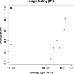
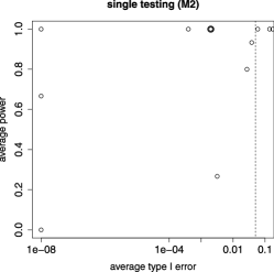
(a)	(b)
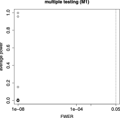
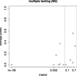
(c)	(d)

Figure 1: Simulated data as described in Section 5.1. (a) and (b): Single testing with average type I error (33) on x-axis (log-scale) and average power (34) on y-axis. (c) and (d): Multiple testing with familywise error rate on x-axis (log-scale) and average power (34), but using $P_{\mathrm{corr};j}$, on y-axis. Vertical dotted line is at abscissa $0.05$. Each point corresponds to a model configuration. (a) and (c): 12 model configurations generated from independent covariates (M1); (b) and (d): 12 model configurations generated from equi-dependent covariates (M2). When an error is zero, we plot it on the log-scale at abscissa $10^{-8}$.

5.2 Values of $P_{\mathbf{X}}$

The detection results in (30) and (4) depend on the ratio $\kappa_{j}=\max_{k\neq j}|(P_{\mathbf{X}})_{jk}|/|(P_{\mathbf{X}})_{jj}|$. We report in Table 1 summary statistics of $\{\kappa_{j}\}_{j}$ for various datasets. We clearly see that the values of $\kappa_{j}$ are typically rather small which implies good detection properties as discussed in Section 4. Furthermore, the values $\max_{k\neq j}|(P_{\mathbf{X}})_{jk}|$ occurring in the construction of $\Delta_{j}$ in Section 2.4.1 are typically very small (not shown here).

Table 1: Minimum, maximum and three quartiles of $\{\kappa_{j}\}_{j=1}^{p}$ for various designs $\mathbf{X}$ from different datasets. The first four are from the simulation models in Section 5.1. Although not relevant for the table, “Motif” (see Section 5.3) and “Riboflavin” have a continuous response while the last six have a class label (Dettling, 2004)

dataset, $(n,p)$	$\min_{j}\kappa_{j}$	$0.25$q$\{\kappa_{j}\}_{j}$	med$\{\kappa_{j}\}_{j}$	$0.75$q$\{\kappa_{j}\}_{j}$	$\max_{j}\kappa_{j}$
(M1), $(100,500)$	0.21	0.27	0.29	0.31	0.44
(M1), $(100,2500)$	0.27	0.34	0.36	0.39	0.54
(M2), $(100,500)$	0.20	0.26	0.29	0.32	0.45
(M2), $(100,2500)$	0.26	0.33	0.36	0.39	0.59
Motif, $(143,287)$	0.05	0.10	0.13	0.18	0.47
Riboflavin, $(71,4088)$	0.29	0.54	0.65	0.77	1.73
Leukemia, $(72,3571)$	0.32	0.44	0.50	0.58	1.57
Colon, $(62,2000)$	0.28	0.50	0.57	0.67	1.36
Lymphoma, $(62,4026)$	0.34	0.52	0.63	0.78	1.49
Brain, $(34,5893)$	0.51	0.63	0.67	0.74	2.44
Prostate, $(102,6033)$	0.26	0.45	0.57	0.74	3.67
NCI, $(61,5244)$	0.37	0.52	0.61	0.79	1.76

5.3 Real data application

We consider a problem about motif regression for finding the binding sites in DNA sequences of the HIF1$\alpha$ transcription factor. The binding sites are also called motifs, and they are typically 6–15 base pairs (with categorical values $\in\{A,C,G,T\}$) long.

The data consists of a univariate response variable $Y$ from CHIP-chip experiments, measuring the logarithm of the binding intensity of the HIF1$\alpha$ transcription factor on coarse DNA segments. Furthermore, for each DNA segment, we have abundance scores for $p=195$ candidate motifs, based on DNA sequence data. Thus, for each DNA segment $i$ we have $Y_{i}\in\mathbb{R}$ and $X_{i}\in\mathbb{R}^{p}$, where $i=1,\ldots,n_{\mathrm{tot}}=287$ and $p=195$. We consider a linear model as in (1) and hypotheses $H_{0,j}$ for $j=1,\ldots,p=195$: rejection of $H_{0,j}$ then corresponds to a significant motif. This dataset has been analyzed in Meinshausen, Meier and Bühlmann (2009) who found one significant motif using their $p$-value method for a linear model based on multiple sample splitting (which assumes the unpleasant “beta-min” condition in (10)).

Since the dataset has $n_{\mathrm{tot}}>p$ observations, we take one random subsample of size $n=143<p=195$. Figure 2 reports the single-testing as well as the adjusted $p$-values for controlling the FWER. There is one significant motif with corresponding FWER-adjusted $p$-value equal to 0.007, and the method in Meinshausen, Meier and Bühlmann (2009) based on the total sample with $n_{\mathrm{tot}}$ found the same significant variable with FWER-adjusted $p$-value equal to 0.006. Interestingly, the weakly significant motif with $p$-value 0.080 is known to be a true binding site for HIF1$\alpha$, thanks to biological validation experiments.

When compared to the Bonferroni–Holm procedure for controlling FWER based on the raw $p$-values as shown in Figure 2(a), we have for the variables with smallest $p$-values:

method as in (28): $$\ 0.007,\ 0.080,\ 0.180,$$

Bonferroni–Holm: $$\ 0.011,\ 0.098,\ 0.242.$$

Thus, for this example, the multiple testing correction as in Section 3 does not provide large improvements in power over the Bonferroni–Holm procedure; but our method is closely related to the Westfall–Young procedure which has been shown to be asymptotically optimal for a broad class of high-dimensional problems (Meinshausen, Maathuis, and Bühlmann, 2011).

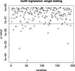
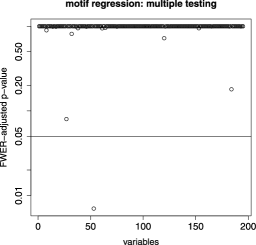
(a)	(b)

Figure 2: Motif regression with $n=143$ and $p=195$. (a) Single-testing $p$-values as in (26); (b) Adjusted $p$-values as in (28) for FWER control. The $p$-values are plotted on the log-scale. Horizontal line is at $y=0.05$.

6 Finite sample results

We present here finite sample analogues of Theorem 1 and 2. Instead of assumption (A), we assume the following:

(A^′)

There are constants $\Delta_{j}>0$ such that

$$\mathbb{P}\biggl{[}\bigcap_{j=1}\biggl{\{}a_{n,p;j}(\sigma)\sum_{k\neq j}(P_{\mathbf{X}})_{jk}\bigl{(}\hat{\beta}_{\mathrm{init};k}-\beta^{0}_{k}\bigr{)}|\leq\Delta_{j}\biggr{\}}\biggr{]}\geq 1-\kappa$$

for some (small) $0<\kappa<1$.

We then have the following result.

Proposition 0.

Assume model (1) with Gaussian errors. Consider the corrected Ridge regression estimator $\hat{\beta}_{\mathrm{corr}}$ in (21) with regularization parameter $\lambda>0$, and assume (16) and condition (A^′). Then, with probability at least $1-\kappa$, for $j\in\{1,\ldots,p\}$ and if $H_{0,j}$ holds:

$$a_{n,p;j}(\sigma)|\hat{\beta}_{\mathrm{corr};j}|\leq a_{n,p;j}(\sigma)|Z_{j}|+\Delta_{j}+\bigl{\|}a_{n,p}b(\lambda)\bigr{\|}_{\infty},$$

$$\bigl{\|}a_{n,p}b(\lambda)\bigr{\|}_{\infty}=\max_{j=1,\ldots,p}a_{n,p;j}(\sigma)\bigl{|}b_{j}(\lambda)\bigr{|}\leq\frac{\lambda}{\Omega_{\mathrm{min}}(\lambda)^{1/2}}n^{1/2}\sigma^{-1}\bigl{\|}\theta^{0}\bigr{\|}_{2}\lambda_{\mathrm{min}\neq 0}(\hat{\Sigma})^{-1}.$$

Similarly, with probability at least $1-\kappa$, for any subset $G\subseteq\{1,\ldots,p\}$ and if $H_{0,G}$ holds:

$$\max_{j\in G}a_{n,p;j}(\sigma)|\hat{\beta}_{\mathrm{corr};j}|\leq\max_{j\in G}\bigl{(}a_{n,p;j}(\sigma)|Z_{j}|+\Delta_{j}\bigr{)}+\bigl{\|}a_{n,p}b(\lambda)\bigr{\|}_{\infty}.$$

A proof is given in Section .1. Due to the third statement in Lemma 1, $\Omega_{\mathrm{min}}(\lambda)^{-1/2}$ is bounded for a bounded range of $\lambda\in(0,C]$. Therefore, the bound for $\|a_{n,p}b(\lambda)\|_{\infty}$ can be made arbitrarily small by choosing $\lambda>0$ sufficiently small.

Theorem 2 is a consequence of the following finite sample result.

Proposition 0.

Consider the event $\mathcal{E}$ with probability $\mathbb{P}[\mathcal{E}]\geq 1-\kappa$ where condition (A^′) holds. Then, when using the corrected $p$-values from (28), with $\zeta\geq 0$ (allowing also $\zeta=0$), we obtain approximate strong control of the familywise error rate:

$$\mathbb{P}[V_{\alpha}>0]\leq F_{Z}\bigl{(}F_{Z}^{-1}(\alpha)-\zeta+2(2\pi)^{-1/2}\bigl{\|}a_{n,p}b(\lambda)\bigr{\|}_{\infty}\bigr{)}+\bigl{(}1-\mathbb{P}[\mathcal{E}]\bigr{)}.$$

A proof is given in Section .1. We immediately get the following bound for $\zeta\geq 0$:

$$\mathbb{P}[V_{\alpha}>0]\leq\alpha+\sup_{u}\bigl{|}F^{\prime}_{Z}(u)\bigr{|}2(2\pi)^{-1/2}\bigl{\|}a_{n,p}b(\lambda)\bigr{\|}_{\infty}+\bigl{(}1-\mathbb{P}[\mathcal{E}]\bigr{)}.$$

7 Conclusions

We have proposed a novel construction of $p$-values for individual and more general hypotheses in a high-dimensional linear model with fixed design and Gaussian errors. We have restricted ourselves to max-type statistics for general hypotheses but modifications to e.g., weighted sums are straightforward using the representation in Proposition 2. A key idea is to use a linear, namely the Ridge estimator, combined with a correction for the potentially substantial bias due to the fact that the Ridge estimator is estimating the projected regression parameter vector onto the row-space of the design matrix. The finding that we can “succeed” with a corrected Ridge estimator in a high-dimensional context may come as a surprise, as it is well known that Ridge estimation can be very bad for say prediction. Nevertheless, our bias corrected Ridge procedure might not be optimal in terms of power, as indicated in Section 4.1. The main assumptions we make are the compatibility condition for the design, i.e., an identifiability condition, and knowledge of an upper bound of the sparsity (see Lemma 2). A related idea of using a linear estimator coupled with a bias correction for deriving confidence intervals has been earlier proposed by Zhang and Zhang (2011).

No tuning parameter. Our approach does not require the specification of a tuning parameter, except for the issue that we crudely bound the true sparsity as in (25); we always used $\xi=0.05$, and the Scaled Lasso initial estimator does not require the specification of a regularization parameter. All our numerical examples were run without tuning the method to a specific setting, and error control with our $p$-value approach is often conservative while the power seems reasonable. Furthermore, our method is generic which allows to test for any $H_{0,G}$ regardless whether the size of $G$ is small or large: we present in the Section .2 an additional simulation where $|G|$ is large. For multiple testing correction or for general hypotheses with sets $G$ where $|G|>1$, we rely on the power of simulation since analytical formulae for max-type statistics under dependence seem in-existing: yet, our simulation is extremely simple as we only need to generate dependent multivariate Gaussian random variables.

Small variance of Ridge estimator. As indicated before, it is surprising that corrected Ridge estimation performs rather well for statistical testing. Although the bias due to the projection $P_{\mathbf{X}}$ can be substantial, it is compensated by small variances $\sigma^{2}n^{-1}\Omega_{jj}$ of the Ridge estimator. It is not true that $\Omega_{jj}$’s become large as $p$ increases: that is, the Ridge estimator has small variance for an individual component when $p$ is very large, see Section 4.1. Therefore, the detection power of the method remains reasonably good as discussed in Section 4. Viewed from a different perspective, even though $|(P_{\mathbf{X}})_{jj}\beta^{0}_{j}|$ may be very small, the normalized version $a_{n,p;j}(\sigma)|(P_{\mathbf{X}})_{jj}\beta^{0}_{j}|$ can be sufficiently large for detection since $a_{n,p;j}(\sigma)$ may be very large (as the inverse of the square root of the variance). The values of $P_{\mathbf{X}}$ can be easily computed for a given problem: our analysis about sufficient conditions for detection in Section 4 could be made more complete by invoking random matrix theory for the projection $P_{\mathbf{X}}$ (assuming that $\mathbf{X}$ is a realization of i.i.d. row-vectors whose entries are potentially dependent). However, currently, most of the results on singular values and similar quantities of $\mathbf{X}$ are for the regime $p\leq n$ (Vershynin, 2012), which leads in our context to the trivial projection $P_{\mathbf{X}}=I$, or for the regime $p/n\to C$ with $0\leq C<\infty$ (El Karoui, 2008).

Extensions. Obvious but partially non-trivial model extensions include random design, non-Gaussian errors or generalized linear models. From a practical point of view, the second and third issue would be most valuable. Relaxing the fixed design assumption makes part of the mathematical arguments more complicated, yet a random design is better posed in terms of identifiability.

Appendix

.1 Proofs

Proof of Proposition 1 The statement about the bias is given in Shao and Deng (2012) (proof of their Theorem 1). The covariance matrix of $\hat{\beta}$ is

$$n^{-1}\Omega=n^{-1}(\hat{\Sigma}+\lambda I)^{-1}\hat{\Sigma}(\hat{\Sigma}+\lambda I)^{-1}.$$

Then, for the variance we obtain $\operatorname{Var}(\hat{\beta}_{j})=n^{-1}\sigma^{2}\Omega_{jj}\geq n^{-1}\sigma^{2}\Omega_{\mathrm{min}}(\lambda)$.

Proof of Proposition 2 We write

$$\hat{\beta}_{\mathrm{corr};j}=\bigl{(}\hat{\beta}_{j}-\mathbb{E}[\hat{\beta}_{j}]\bigr{)}+\theta^{0}_{j}-\sum_{k\neq j}(P_{\mathbf{X}})_{jk}\hat{\beta}_{\mathrm{init};k}+\bigl{(}\mathbb{E}[\hat{\beta}_{j}]-\theta^{0}_{j}\bigr{)}.$$

The result then follows by defining $Z_{j}=\hat{\beta}_{j}-\mathbb{E}[\hat{\beta}_{j}]$ and using that $\theta^{0}_{j}=(P_{\mathbf{X}}\beta^{0})_{j}=(P_{\mathbf{X}})_{jj}\beta^{0}_{j}+\sum_{k\neq j}(P_{\mathbf{X}})_{jk}\beta^{0}_{k}$.

Proof of Proposition 3 (basis for proving Theorem 1) The bound from Proposition 1 for the estimation bias of the Ridge estimator leads to:

$$\bigl{\|}a_{n,p}b(\lambda)\bigl{\|}_{\infty} = \max_{j=1,\ldots,p}a_{n,p;j}(\sigma)\bigl{|}\mathbb{E}[\hat{\beta}_{j}]-\theta^{0}_{j}\bigr{|}$$

$$\leq \frac{\lambda\|\theta^{0}\|_{2}\lambda_{\mathrm{min}\neq 0}(\hat{\Sigma})^{-1}}{\sigma n^{-1/2}\Omega_{jj}^{1/2}}$$

$$\leq \lambda\bigl{\|}\theta^{0}\bigl{\|}_{2}\lambda_{\mathrm{min}\neq 0}(\hat{\Sigma})^{-1}\sigma^{-1}n^{1/2}\Omega_{\mathrm{min}}(\lambda)^{-1/2}.$$

By using the representation from Proposition 2, invoking assumption (A^′) and assuming that the null-hypothesis $H_{0,j}$ or $H_{0,G}$ holds, respectively, the proof is completed.

Proof of Theorem 1 Due to the choice of $\lambda=\lambda_{n}$ we have that $\|a_{n,p}b(\lambda_{n})\|_{\infty}=o(1)\ (n\to\infty)$. The proof then follows from Proposition 3 and invoking assumption (A) saying that the probabilities for the statements in Proposition 3 converge to 1 as $n\to\infty$.

Proof of Proposition 4 (basis for proving Theorem 2) Consider the set $\mathcal{E}$ where assumption (A^′) holds (whose probability is at least $\mathbb{P}[\mathcal{E}]\geq 1-\kappa$). Without loss of generality, we consider $P_{j}=2(1-\Phi(a_{n,p;j}(\sigma)|\hat{\beta}_{\mathrm{corr};j}|-\Delta_{j}))$ without the truncation at value 1 (implied by the positive part $(a_{n,p;j}(\sigma)|\hat{\beta}_{\mathrm{corr};j}|-\Delta_{j})_{+}$); in terms of decisions (rejection or non-rejection of a hypothesis), both versions for the $p$-value are equivalent. Then, on $\mathcal{E}$ and for $j\in S_{0}^{c}$:

$$P_{j} = 2\bigl{(}1-\Phi\bigl{(}a_{n,p;j}(\sigma)|\hat{\beta}_{\mathrm{corr};j}|-\Delta_{j}\bigr{)}\bigr{)}$$

$$\geq 2\biggl{(}1-\Phi\biggl{(}a_{n,p;j}(\sigma)\biggl{|}\hat{\beta}_{\mathrm{corr};j}-\sum_{k\neq j}(P_{\mathbf{X}})_{jk}\bigl{(}\hat{\beta}_{\mathrm{init};k}-\beta^{0}_{k}\bigr{)}\biggr{|}\biggr{)}\biggr{)}$$

$$\geq 2\bigl{(}1-\Phi\bigl{(}a_{n,p;j}(\sigma)|Z_{j}|\bigr{)}\bigr{)}-2(2\pi)^{-1/2}\bigl{\|}a_{n,p}b(\lambda)\bigr{\|}_{\infty},$$

where in the last inequality we used Proposition 2 and Taylor’s expansion. Thus, on $\mathcal{E}$:

$$\min_{j\in S_{0}^{c}}P_{j} \geq \min_{j\in S_{0}^{c}}2\bigl{(}1-\Phi\bigl{(}a_{n,p;j}(\sigma)|Z_{j}|\bigr{)}\bigr{)}-2(2\pi)^{-1/2}\bigl{\|}a_{n,p}b(\lambda)\bigr{\|}_{\infty}$$

$$\geq \min_{j=1,\ldots,p}2\bigl{(}1-\Phi\bigl{(}a_{n,p;j}(\sigma)|Z_{j}|\bigr{)}\bigr{)}-2(2\pi)^{-1/2}\bigl{\|}a_{n,p}b(\lambda)\bigr{\|}_{\infty}.$$

Therefore,

$$\mathbb{P}\Bigl{[}\min_{j\in S_{0}^{c}}P_{j}\leq c\Bigr{]} \leq \mathbb{P}\Bigl{[}\mathcal{E}\cap\Bigl{\{}\min_{j\in S_{0}^{c}}P_{j}\leq c\Bigr{\}}\Bigr{]}+\mathbb{P}\bigl{[}\mathcal{E}^{c}\bigr{]}$$

$$\leq \mathbb{P}\Bigl{[}\min_{j=1,\ldots,p}2\bigl{(}1-\Phi\bigl{(}a_{n,p;j}(\sigma)|Z_{j}|\bigr{)}\bigr{)}\leq c+2(2\pi)^{-1/2}\bigl{\|}a_{n,p}b(\lambda)\bigr{\|}_{\infty}\Bigr{]}+\mathbb{P}\bigl{[}\mathcal{E}^{c}\bigr{]}$$

$$= F_{Z}\bigl{(}c+2(2\pi)^{-1/2}\bigl{\|}a_{n,p}b(\lambda)\bigr{\|}_{\infty}\bigr{)}+\mathbb{P}\bigl{[}\mathcal{E}^{c}\bigr{]}.$$

Using this we obtain:

$$\mathbb{P}[V_{\alpha}>0] = \mathbb{P}\Bigl{[}\min_{j\in S_{0}^{c}}P_{\mathrm{corr};j}\leq\alpha\Bigr{]}=\mathbb{P}\Bigl{[}\min_{j\in S_{0}^{c}}P_{j}\leq F_{Z}^{-1}(\alpha)-\zeta\Bigr{]}$$

$$\leq F_{Z}\bigl{(}F_{Z}^{-1}(\alpha)-\zeta+2(2\pi)^{-1/2}\bigl{\|}a_{n,p}b(\lambda)\bigr{\|}_{\infty}\bigr{)}+\mathbb{P}\bigl{[}\mathcal{E}^{c}\bigr{]}.$$

This completes the proof.

Proof of Theorem 2 Due to the choice of $\lambda=\lambda_{n}$ we have that $\|a_{n,p}b(\lambda_{n})\|_{\infty}=o(1)\ (n\to\infty)$. Furthermore, using the formulation in Proposition 4, assumption (A) translates to a sequence of sets $\mathcal{E}_{n}$ with $\mathbb{P}[\mathcal{E}_{n}]\to 1\ (n\to\infty)$. We then use Proposition 4 and observe that for sufficiently large $n$: $F_{Z}(F_{Z}^{-1}(\alpha)-\zeta+2(2\pi)^{-1/2}\|a_{n,p}b(\lambda_{n})\|_{\infty})\leq F_{Z}(F_{Z}^{-1}(\alpha))\leq\alpha$. The modification for the case with $\alpha_{n}\to 0$ sufficiently slowly follows analogously: note that the second last inequality in the proof above follows by monotonicity of $F_{Z}(\cdot)$ and $\zeta>2(2\pi)^{-1/2}\|a_{n,p}b(\lambda_{n})\|_{\infty}$ for $n$ sufficiently large. This completes the proof.

Proof of Theorem 3 Throughout the proof, $\alpha_{n}\to 0$ is converging sufficiently slowly, possibly depending on the context of the different statements we prove. Regarding statement 1: it is sufficient that for $j\in S_{0}$,

$$a_{n,p;j}(\sigma)|\hat{\beta}_{\mathrm{corr};j}|\gg\max(\Delta_{j},1).$$

From Proposition 2, we see that this can be enforced by requiring

$$a_{n,p;j}(\sigma)\biggl{(}\bigl{|}(P_{\mathbf{X}})_{jj}\beta^{0}_{j}\bigr{|}-\biggl{|}\sum_{k\neq j}(P_{\mathbf{X}})_{jk}\bigl{(}\hat{\beta}_{\mathrm{init};k}-\beta^{0}_{k}\bigr{)}\biggr{|}-|Z_{j}|-\bigl{|}b_{j}(\lambda)\bigr{|}\biggr{)}\gg\max(\Delta_{j},1).$$

Since $|a_{n,p;j}(\sigma)\sum_{k\neq j}(P_{\mathbf{X}})_{jk}(\hat{\beta}_{\mathrm{init};k}-\beta^{0}_{k})|\leq\Delta_{j}$, this holds if

$$\bigl{|}\beta^{0}_{j}\bigr{|}\gg\frac{1}{|(P_{\mathbf{X}})_{jj}|a_{n,p;j}(\sigma)}\max\bigl{(}\Delta_{j},a_{n,p;j}(\sigma)Z_{j},a_{n,p;j}(\sigma)b_{j}(\lambda),1\bigr{)}.$$ (35)

Due to the choice of $\lambda=\lambda_{n}$ (as in Theorem 1), we have $a_{n,p;j}(\sigma)b_{j}(\lambda)\leq\|a_{n,p}(\sigma)b(\lambda)\|_{\infty}=o(1)$. Hence, (35) holds with probability converging to one if

$$\bigl{|}\beta^{0}_{j}\bigr{|}\gg\frac{1}{|(P_{\mathbf{X}})_{jj}|a_{n,p;j}(\sigma)}\max(\Delta_{j},1),$$

completing the proof for statement 1.

For proving the second statement, we recall that

$$1-J_{G}(c)=\mathbb{P}\Bigl{[}\max_{j\in G}\bigl{(}a_{n,p;j}(\sigma)|Z_{j}|+\Delta_{j}\bigr{)}>c\Bigr{]}.$$

Denote by $W=\max_{j\in G}(a_{n,p;j}(\sigma)|Z_{j}|+\Delta_{j})\leq\tilde{W}=\max_{j\in G}a_{n,p;j}(\sigma)|Z_{j}|+\max_{j\in G}\Delta_{j}$. Thus,

$$\mathbb{P}[W>c]\leq\mathbb{P}[\tilde{W}>c].$$

Therefore, the statement for the $p$-value $\mathbb{P}[P_{G}\leq\alpha_{n}]$ is implied by

$$\mathbb{P}_{\tilde{W}}[\tilde{W}>\hat{\gamma}_{G}]\leq\alpha_{n}.$$ (36)

Using the union bound and the fact that $a_{n,p;j}(\sigma)|Z_{j}|\sim\mathcal{N}(0,1)$ (but dependent over different values of $j$), we have that

$$\max_{j\in G}a_{n,p;j}(\sigma)|Z_{j}|=O_{P}\bigl{(}\sqrt{\log\bigl{(}|G|\bigr{)}}\bigr{)}.$$

Therefore, (36) holds if

$$\hat{\gamma}_{G}=\max_{j\in G}a_{n,p;j}(\sigma)|\hat{\beta}_{\mathrm{corr};j}|\gg\max\Bigl{(}\max_{j\in G}\Delta_{j},\sqrt{\log\bigl{(}|G|\bigr{)}}\Bigr{)}.$$

The argument is now analogous to the proof of the first statement above, using the representation from Proposition 2.

Regarding the third statement, we invoke the rough bound

$$P_{\mathrm{corr};j}\leq pP_{j},$$

with the non-truncated Bonferroni corrected $p$-value at the right-hand side. Hence,

$$\max_{j\in S_{0}}P_{\mathrm{corr};j}\leq\alpha_{n}$$

is implied by

$$\max_{j\in S_{0}}pP_{j}=\max_{j\in S_{0}}2p\bigl{(}1-\Phi\bigl{(}\bigl{(}a_{n,p;j}(\sigma)|\hat{\beta}_{\mathrm{corr};j}|-\Delta_{j}\bigr{)}_{+}\bigr{)}\bigr{)}\leq\alpha_{n}.$$

Since this involves a standard Gaussian two-sided tail probability, the inequality can be enforced (for certain slowly converging $\alpha_{n}$) by

$$\max_{j\in S_{0}}2\exp\bigl{(}\log(p)-\bigl{(}a_{n,p;j}(\sigma)|\hat{\beta}_{\mathrm{corr};j}|-\Delta_{j}\bigr{)}_{+}^{2}/2\bigr{)}=o_{P}(1).$$

The argument is now analogous to the proof of the first statement above, using the representation from Proposition 2.

The fourth statement involves slight obvious modifications of the arguments above.

.2 $P$-values for $H_{0,G}$ with $|G|$ large

We report here on a small simulation study for testing $H_{0,G}$ with $G=\{1,2,\ldots,100\}$. We consider model (M2) from Section 5.1 with 4 different configurations and we use the $p$-value from (27) with corresponding decision rule for rejection of $H_{0,G}$ if the $p$-value is smaller or equal to the nominal level 0.05. Table 2 describes the result based on 500 independent simulations (where the fixed design remains the same). The method works well with much better power than multiple testing of individual hypotheses but worse than average power for testing individual hypotheses without multiplicity adjustment (which is not a proper approach). This is largely in agreement with the theoretical results in Theorem 3. Furthermore, the type I error control is good.

Table 2: Testing of general hypothesis $H_{0,G}$ with $|G|=100$ using the $p$-value in (27) with significance level $0.05$. Second column: type I error; Third column: power; Fourth column: comparison with power using multiple individual testing and average power using individual testing without multiplicity adjustment (both for all $p$ hypotheses $H_{0,j}\ (j=1,\ldots,p)$)

Model	$\mathbb{P}[\mbox{false rejection}]$	$\mathbb{P}[\mbox{true rejection}]$	(power mult., power indiv.)
(M2), $p=500$, $s=3$, $b=0.5$	0.00	0.10	(0.01,1.00)
(M2), $p=500$, $s=3$, $b=1$	0.00	0.91	(0.37,1.00)
(M2), $p=2500$, $s=3$, $b=0.5$	0.01	0.02	(0.00,1.00)
(M2), $p=2500$, $s=3$, $b=1$	0.00	0.83	(0.17,1.00)

.3 Number of false positives in simulated examples

We show in Table 3 the number of false positives $V=V_{0.05}$ in the simulated scenarios where the FWER (among individual hypotheses) was found too large. Although the FWER is larger than 0.05, the number of false positives is relatively small, except for the extreme model (M2), $p=2500$, $s=15$, $b=1$ which has a too large sparsity and a too strong signal strength. For the latter model, we would need to increase $\xi$ in (25) to achieve better error control.

Table 3: Probabilities for false positives for simulation models from Section 5.1 in scenarios where the FWER is clearly overshooting the nominal level $0.05$

Model	$\mathbb{P}[V=0]$	$\mathbb{P}[V=1]$	$\mathbb{P}[V=2]$	$\mathbb{P}[V=3]$	$\mathbb{P}[V=4]$	$\mathbb{P}[V\geq 5]$
(M2), $p=500$, $s=15$, $b=1$	0.482	0.336	0.138	0.028	0.010	0.006
(M2), $p=500$, $s=15$, $b=0.5$	0.746	0.218	0.034	0.000	0.002	0.000
(M2), $p=2500$, $s=15$, $b=1$	0.012	0.044	0.098	0.126	0.172	0.548
(M2), $p=2500$, $s=15$, $b=0.5$	0.504	0.328	0.132	0.032	0.004	0.000

.4 Further discussion about $p$-values and bounds $\Delta_{j}$ in assumption (A)

The $p$-values in (26) and (27) are crucially based on the idea of correction with the bounds $\Delta_{j}$ in Section 2.4.1. The essential idea is contained in Proposition 2:

$$a_{n,p;j}(\sigma)\hat{\beta}_{\mathrm{corr};j}$$

$$\quad=a_{n,p;j}(\sigma)(P_{\mathbf{X}})_{jj}-a_{n,p;j}(\sigma)\sum_{k\neq j}(P_{\mathbf{X}})_{jk}\bigl{(}\hat{\beta}_{\mathrm{init};k}-\beta^{0}_{k}\bigr{)}+a_{n,p;j}(\sigma)Z_{j}+\mbox{negligible term}.$$

There are three cases. If

$$a_{n,p;j}(\sigma)\sum_{k\neq j}(P_{\mathbf{X}})_{jk}\bigl{(}\hat{\beta}_{\mathrm{init};k}-\beta^{0}_{k}\bigr{)}=o_{P}(1),$$ (37)

a correction with the bound $\Delta_{j}$ would not be necessary, but of course, it does not hurt in terms of type I error control. If

$$a_{n,p;j}(\sigma)\sum_{k\neq j}(P_{\mathbf{X}})_{jk}\bigl{(}\hat{\beta}_{\mathrm{init};k}-\beta^{0}_{k}\bigr{)}\asymp V,$$ (38)

for some non-degenerate random variable $V$, the correction with the bound $\Delta_{j}$ is necessary and assuming that $\Delta_{j}$ is of the same order of magnitude as $V$, we have a balance between $\Delta_{j}$ and the stochastic term $a_{n,p;j}(\sigma)Z_{j}$. In the last case where

$$a_{n,p;j}(\sigma)\sum_{k\neq j}(P_{\mathbf{X}})_{jk}\bigl{(}\hat{\beta}_{\mathrm{init};k}-\beta^{0}_{k}\bigr{)}\to\infty,$$ (39)

the bound $\Delta_{j}$ would be the dominating element in the $p$-value construction. We show in Figure 3 that there is empirical evidence that (38) applies most often.

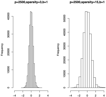
Figure 3: Histogram of projection bias $a_{n,p;j}(\sigma)\sum_{k\neq j}(P_{\mathbf{X}})_{jk}(\hat{\beta}_{\mathrm{init};k}-\beta^{0}_{k})$ over all values $j=1,\ldots,p$ and over 100 independent simulation runs. Left: model (M2), $p=2500$, $s=3$, $b=1$; Right: model (M2), $p=2500$, $s=15$, $b=1$.

Case (39) is comparable to a crude procedure which makes a hard decision about relevance of the underlying coefficients:

$$\mbox{if }a_{n,p;j}(\sigma)|\hat{\beta}_{\mathrm{corr};j}|>\Delta_{j}\mbox{ holds, then $H_{0,j}$ is rejected},$$

and the rejection would be “certain” corresponding to a $p$-value with value equal to $0$; and in case of a “$\leq$” relation, the corresponding $p$-value would be set to one. This is an analogue to the thresholding rule:

$$\mbox{if}\ |\hat{\beta}_{\mathrm{init};j}|>\Delta_{\mathrm{init}}\ \mbox{holds, then $H_{0,j}$ is rejected},$$ (40)

where $\Delta_{\mathrm{init}}\geq\|\hat{\beta}_{\mathrm{init}}-\beta^{0}\|_{\infty}$, e.g. using a bound where $\Delta_{\mathrm{init}}\geq\|\hat{\beta}_{\mathrm{init}}-\beta^{0}\|_{1}$. For example, (40) could be the variable selection estimator with the thresholded Lasso procedure (van de Geer, Bühlmann and Zhou, 2011). An accurate construction of $\Delta_{\mathrm{init}}$ for practical use is almost impossible: it depends on $\sigma$ and in a complicated way on the nature of the design through e.g. the compatibility constant, see (7).

Our proposed bound $\Delta_{j}$ in (25) is very simple. In principle, its justification also depends on a bound for $\|\hat{\beta}_{\mathrm{init}}-\beta^{0}\|_{1}$, but with the advantage of “robustness”. First, the bound $a_{n,p;j}(\sigma)\max_{k\neq j}|(P_{\mathbf{X}})_{jk}|\|\hat{\beta}_{\mathrm{init}}-\beta^{0}\|_{1}$ appearing in (23) is not depending on $\sigma$ anymore (since $\|\hat{\beta}_{\mathrm{init}}-\beta^{0}\|_{1}$ scales linearly with $\sigma$). Secondly, the inequality in (23) is crude implying that $\Delta_{j}$ in (25) may still satisfy assumption (A) even if the bound of $\|\hat{\beta}_{\mathrm{init}}-\beta^{0}\|_{1}$ is misspecified and too small. The construction of $p$-values as in (26) and (27) is much better for practical purposes (and for simulated examples) than using a rule as in (40).

References

- Bickel, Ritov and Tsybakov (2009) {barticle}[mr] \bauthor\bsnmBickel, \bfnmPeter J.\binitsP.J., \bauthor\bsnmRitov, \bfnmYa’acov\binitsY. &\bauthor\bsnmTsybakov, \bfnmAlexandre B.\binitsA.B. (\byear2009). \btitleSimultaneous analysis of lasso and Dantzig selector. \bjournalAnn. Statist. \bvolume37 \bpages1705–1732. \biddoi=10.1214/08-AOS620, issn=0090-5364, mr=2533469 \bptokimsref \endbibitem
- Bickel et al. (1998) {bbook}[mr] \bauthor\bsnmBickel, \bfnmPeter J.\binitsP.J., \bauthor\bsnmKlaassen, \bfnmChris A. J.\binitsC.A.J., \bauthor\bsnmRitov, \bfnmYa’acov\binitsY. &\bauthor\bsnmWellner, \bfnmJohn A.\binitsJ.A. (\byear1998). \btitleEfficient and Adaptive Estimation for Semiparametric Models. \blocationNew York: \bpublisherSpringer. \bidmr=1623559 \bptokimsref \endbibitem
- Bühlmann (2006) {barticle}[mr] \bauthor\bsnmBühlmann, \bfnmPeter\binitsP. (\byear2006). \btitleBoosting for high-dimensional linear models. \bjournalAnn. Statist. \bvolume34 \bpages559–583. \biddoi=10.1214/009053606000000092, issn=0090-5364, mr=2281878 \bptokimsref \endbibitem
- Bühlmann, Kalisch and Maathuis (2010) {barticle}[mr] \bauthor\bsnmBühlmann, \bfnmP.\binitsP., \bauthor\bsnmKalisch, \bfnmM.\binitsM. &\bauthor\bsnmMaathuis, \bfnmM. H.\binitsM.H. (\byear2010). \btitleVariable selection in high-dimensional linear models: Partially faithful distributions and the PC-simple algorithm. \bjournalBiometrika \bvolume97 \bpages261–278. \biddoi=10.1093/biomet/asq008, issn=0006-3444, mr=2650737 \bptokimsref \endbibitem
- Bühlmann and van de Geer (2011) {bbook}[mr] \bauthor\bsnmBühlmann, \bfnmPeter\binitsP. &\bauthor\bparticlevan de \bsnmGeer, \bfnmSara\binitsS. (\byear2011). \btitleStatistics for High-dimensional Data: Methods, Theory and Applications. \bseriesSpringer Series in Statistics. \blocationHeidelberg: \bpublisherSpringer. \biddoi=10.1007/978-3-642-20192-9, mr=2807761 \bptokimsref \endbibitem
- Bunea, Tsybakov and Wegkamp (2007) {barticle}[mr] \bauthor\bsnmBunea, \bfnmFlorentina\binitsF., \bauthor\bsnmTsybakov, \bfnmAlexandre\binitsA. &\bauthor\bsnmWegkamp, \bfnmMarten\binitsM. (\byear2007). \btitleSparsity oracle inequalities for the Lasso. \bjournalElectron. J. Stat. \bvolume1 \bpages169–194. \biddoi=10.1214/07-EJS008, issn=1935-7524, mr=2312149 \bptokimsref \endbibitem
- Candes and Tao (2007) {barticle}[mr] \bauthor\bsnmCandes, \bfnmEmmanuel\binitsE. &\bauthor\bsnmTao, \bfnmTerence\binitsT. (\byear2007). \btitleThe Dantzig selector: Statistical estimation when is much larger than . \bjournalAnn. Statist. \bvolume35 \bpages2313–2351. \biddoi=10.1214/009053606000001523, issn=0090-5364, mr=2382644 \bptnotecheck related\bptokimsref \endbibitem
- Dettling (2004) {barticle}[pbm] \bauthor\bsnmDettling, \bfnmMarcel\binitsM. (\byear2004). \btitleBagBoosting for tumor classification with gene expression data. \bjournalBioinformatics \bvolume20 \bpages3583–3593. \biddoi=10.1093/bioinformatics/bth447, issn=1367-4803, pii=bth447, pmid=15466910 \bptokimsref \endbibitem
- El Karoui (2008) {barticle}[mr] \bauthor\bsnmEl Karoui, \bfnmNoureddine\binitsN. (\byear2008). \btitleSpectrum estimation for large dimensional covariance matrices using random matrix theory. \bjournalAnn. Statist. \bvolume36 \bpages2757–2790. \biddoi=10.1214/07-AOS581, issn=0090-5364, mr=2485012 \bptokimsref \endbibitem
- Fan and Li (2001) {barticle}[mr] \bauthor\bsnmFan, \bfnmJianqing\binitsJ. &\bauthor\bsnmLi, \bfnmRunze\binitsR. (\byear2001). \btitleVariable selection via nonconcave penalized likelihood and its oracle properties. \bjournalJ. Amer. Statist. Assoc. \bvolume96 \bpages1348–1360. \biddoi=10.1198/016214501753382273, issn=0162-1459, mr=1946581 \bptokimsref \endbibitem
- Fan and Lv (2008) {barticle}[mr] \bauthor\bsnmFan, \bfnmJianqing\binitsJ. &\bauthor\bsnmLv, \bfnmJinchi\binitsJ. (\byear2008). \btitleSure independence screening for ultrahigh dimensional feature space. \bjournalJ. R. Stat. Soc. Ser. B Stat. Methodol. \bvolume70 \bpages849–911. \biddoi=10.1111/j.1467-9868.2008.00674.x, issn=1369-7412, mr=2530322 \bptnotecheck related\bptokimsref \endbibitem
- Fan and Lv (2010) {barticle}[mr] \bauthor\bsnmFan, \bfnmJianqing\binitsJ. &\bauthor\bsnmLv, \bfnmJinchi\binitsJ. (\byear2010). \btitleA selective overview of variable selection in high dimensional feature space. \bjournalStatist. Sinica \bvolume20 \bpages101–148. \bidissn=1017-0405, mr=2640659 \bptokimsref \endbibitem