BCS-BEC crossover in three-dimensional Fermi gases with spherical spin-orbit coupling

Abstract

We present a systematic theoretical study of the BCS-BEC crossover problem in three-dimensional atomic Fermi gases at zero temperature with a spherical spin-orbit coupling which can be generated by a synthetic non-Abelian gauge field coupled to neutral fermions. Our investigations are based on the path integral formalism which is a powerful theoretical scheme for the study of the properties of the bound state, the superfluid ground state, and the collective excitations in the BCS-BEC crossover. At large spin-orbit coupling, the system enters the BEC state of a novel type of bound state (referred to as rashbon) which possesses a non-trivial effective mass. Analytical results and interesting universal behaviors for various physical quantities at large spin-orbit coupling are obtained. Our theoretical predictions can be tested in future experiments of cold Fermi gases with three-dimensional spherical spin-orbit coupling.

I Introduction

It has been widely accepted for a long time that, by tuning the attractive strength in a Fermi gas, one can realize a smooth crossover from the Bardeen–Cooper–Schrieffer (BCS) superfluidity at weak attraction to Bose–Einstein condensation (BEC) of difermion molecules at strong attraction Eagles ; Leggett ; BCSBEC1 ; BCSBEC2 ; BCSBEC3 ; BCSBEC4 ; BCSBEC5 ; BCSBEC6 ; BCSBEC7 . For a dilute Fermi gas in three dimensions where the effective range $r_{0}$ of the short-range interaction is much smaller than the inter-particle distance, the system can be characterized by a dimensionless parameter $1/(k_{\rm F}a_{s})$, where $a_{s}$ is the $s$-wave scattering length of the short-range interaction and $k_{\rm F}$ is the Fermi momentum in the absence of interaction. The BCS-BEC crossover occurs when the parameter $1/(k_{\rm F}a_{s})$ is tuned from negative to positive values, and the BCS and BEC limits correspond to the cases $1/(k_{\rm F}a_{s})\rightarrow-\infty$ and $1/(k_{\rm F}a_{s})\rightarrow+\infty$, respectively. The BCS-BEC crossover has also become an interesting issue for the studies of dense nuclear and quark matter which may exists in the core of compact stars BCSBECNM ; BCSBECHe ; BCSBECQM .

This BCS-BEC crossover phenomenon has been successfully demonstrated in ultracold fermionic atoms, where the $s$-wave scattering length and hence the parameter $1/(k_{\rm F}a_{s})$ were tuned by means of the Feshbach resonance BCSBECexp1 ; BCSBECexp2 ; BCSBECexp3 . At the resonant point or the so-called unitary point where $a_{s}\rightarrow\infty$, the only length scale of the system is the inter-particle distance ($\sim k_{\rm F}^{-1}$). Therefore, the properties of the system at the unitary point $1/(k_{\rm F}a_{s})=0$ become universal, i.e., independent of the details of the interactions. All physical quantities, scaled by their counterparts for the non-interacting Fermi gases, become universal constants. Determining these universal constants has been one of the most intriguing topics in the research of the cold Fermi gases Unitary ; Unitary2 .

While the BCS-BEC crossover triggered by tuning the attraction strength between fermions from weak to strong ($1/(k_{\rm F}a_{s})$ from $-\infty$ to $+\infty$) has been comprehensively studied both theoretically and experimentally, it is always interesting to look for other mechanisms to realize the BCS-BEC crossover. Recent experimental breakthrough in generating synthetic non-Abelian gauge field SOC has opened up the opportunity to study the spin-orbit coupling (SOC) effect in cold atomic gases SOC01 ; SOC02 ; SOC03 ; SOC04 ; 3DSOC . For fermionic atoms, it may provide an alternative way to realize the BCS-BEC crossover 3DBCSBEC . Apart from engineering cold-atom analogs to known Hamitonians such as Rashba SOC, synthetic non-Abelian gauge field can generate SOC that has no known analog in condensed matter systems.

The spin-orbit coupling for neutral fermions can be generated by a synthetic SU(2) gauge field. In general, the synthetic vector potential ${\bf A}$ for spin-1/2 fermions takes the form ${\bf A}=-(\lambda_{x}\sigma_{x}{\bf e}_{x}+\lambda_{y}\sigma_{y}{\bf e}_{y}+\lambda_{z}\sigma_{z}{\bf e}_{z})$ SOC03 ; SOC04 ; 3DSOC ; 3Dbound , where $\sigma_{i}$ ($i=x,y,z$) are the Pauli matrices. From the minimum coupling scheme, the resulting Hamiltonian for spin-1/2 fermions moving in a gauge potential ${\bf A}$ reads ${\cal H}={\bf p}^{2}/(2m)+\mbox{\boldmath{$\sigma$}}\cdot\mbox{\boldmath{$\xi$}}_{\lambda}$ where $\mbox{\boldmath{$\xi$}}_{\lambda}=(\lambda_{x}p_{x},\lambda_{y}p_{y},\lambda_{z}p_{z})$. The term $\mbox{\boldmath{$\sigma$}}\cdot\mbox{\boldmath{$\xi$}}_{\lambda}$ can be regarded as a generalized Rashba SOC. The gauge field strengths $\lambda_{i}$ ($i=x,y,z$) characterize the spin-orbital coupling constants. The problem of the difermion bound state in the three-dimensional (3D) case in the presence of SOC has been studied in Ref. 3Dbound . Three special cases were considered: (1) $\lambda_{x}=\lambda_{y}=0$ and $\lambda_{z}=\lambda$ (called extreme prolate (EP)); (2) $\lambda_{x}=\lambda_{y}=\lambda$ and $\lambda_{z}=0$ (called extreme oblate (EO)); (3) $\lambda_{x}=\lambda_{y}=\lambda_{z}=\lambda$ (called spherical (S)). The EO-type SOC is physically equivalent to the Rashba SOC which is interesting for condensed matter physics. For EO- and S-type SOCs, it was shown that the difermion bound state exists even for $a_{s}<0$ where the bound state does not exist in the absence of SOC. With increased SOC, the binding energy is generally enhanced3Dbound . The bound state also possesses a non-trivial effective mass which is generally larger than twice of the fermion mass $m$ 3D1 ; rashbon ; Iskin . Such a novel bound state caused by the SOC is now referred to as rashbons in the literatures rashbon . For the two-dimensional (2D) case, the bound state exists for arbitrarily small attraction. It was shown in Ref. 2Dhe that the EO-type SOC or the Rashba SOC enhances the binding energy and the bound state also has a non-trivial effective mass. This is analogous to the catalysis of the dynamical mass generation by an external non-Abelian gauge field in quantum field theory NJL .

Because of the presence of novel bound state with SOC, it has been proposed that a dilute Fermi gas with EO- and S-type SOCs can undergo a smooth crossover from the BCS superfluid state to the Bose-Einstein condensation of rashbons (RBEC) even for negative values of $1/(k_{\rm F}a_{s})$ if the SOC constant $\lambda$ is tuned from small to large values 3DBCSBEC . Due to the presence of SOC constant $\lambda$, the 3D BCS-BEC crossover problem depends on two dimensionless parameters: $1/(k_{\rm F}a_{s})$ and $\lambda/k_{\rm F}$ (we set $m=1$ in this paper). The BCS-BEC crossover problem and anisotropic superfluidity in 3D Fermi gases with EO-type SOC has been extensively studied 3D1 ; 3D2 . It was shown that the system enters the RBEC regime at $\lambda/k_{\rm F}\sim 1$ for EO-type SOC for negative values of $1/(k_{\rm F}a_{s})$. The BCS-BEC crossover in 2D Fermi gases with EO-type SOC was also studied 2Dhe ; chen . Similar conclusions were found for the 2D case.

In this paper, we present a systematic theoretical study of the BCS-BEC crossover in 3D Fermi gases at zero temperature with S-type SOC. Especially, we will study the properties of the collective modes along the BCS-BEC crossover and the effective interaction among the rashbons in the RBEC regime. As far as we know, in the presence of SOC, these two interesting issues have not yet been studied (See the Note added). For S-type SOC, the superfluid ground state is isotropic, which brings much convenience to the computations, and enables us to obtain various analytical results and universal behaviors at large SOC.

This paper is organized as follows. In Sec. II, we set up the functional path integral formalism for the BCS-BEC crossover problem with a spherical SOC. Then we first determine the binding energy and the effective mass of the rashbon at vanishing density and temperature (the vacuum in the presence of SOC) in Sec. III. The ground state properties, such as the solution of the gap and number equations, fermion momentum distribution, the condensate fraction, and the superfluid density are discussed in Sec. IV. We derive the Gross-Pitaevskii free energy for the weakly interacting rashbon condensate at large SOC and determine the rashbon-rashbon scattering length in Sec. V. The properties of the collective excitations, such as the gapless Goldstone mode and the massive Anderson-Higgs mode, are investigated in Sec. VI. We summarize in Sec. VII.

II Model and Effective Potential

For neutral atoms, the spin-orbit coupling can be generated by a synthetic non-Abelian gauge potential ${\bf A}$. For instance, the well-known Rashba spin-orbit coupling in solid-state systems can be generated via a 2D synthetic vector potential SOC03 ; SOC04

$${\bf A}=-\lambda(\sigma_{x}{\bf e}_{x}+\sigma_{y}{\bf e}_{y}).$$ (1)

For spin-1/2 fermions moving in three spatial dimensions, this results in an anisotropic (but circular in $x$-$y$ plane) ground state.

In this paper, we are interested in a 3D extension of the Rashba spin-orbit coupling. A 3D synthetic vector potential ${\bf A}$ can be produced by laser-induced coupling to link four internal atomic states with a tetrahedral geometry 3DSOC . The synthetic 3D vector potential takes the form 3DSOC

$${\bf A}=-\lambda_{\perp}(\sigma_{x}{\bf e}_{x}+\sigma_{y}{\bf e}_{y})-\lambda_{\parallel}\sigma_{z}{\bf e}_{z},$$ (2)

which includes all three components of the Pauli matrices. The single-particle Hamiltonian describing spin-1/2 fermions moving in three spatial dimensions in the synthetic gauge field is given by

$${\cal H}_{\text{GF}}=\frac{\left(\hat{\bf p}-{\bf A}\right)^{2}}{2m},$$ (3)

where $\hat{\bf p}=-i\hbar\nabla$ is the momentum operator. In the following we use the natural units $\hbar=k_{\text{B}}=m=1$. We are interested in the fully spherical case, $\lambda_{\perp}=\lambda_{\parallel}\equiv\lambda$. The single-particle Hamiltonian can be reduced to

$${\cal H}_{\text{GF}}=\frac{\hat{\bf p}^{2}}{2}+\lambda\mbox{\boldmath{$\sigma$}}\cdot\hat{\bf p},$$ (4)

where an irrelevant constant $\lambda^{2}/2$ has been omitted. The resulting spherical SOC term $\lambda\mbox{\boldmath{$\sigma$}}\cdot\hat{\bf p}$ can be called a Weyl spin-orbit coupling 3DSOC in analogy to the Weyl fermions weyl . Here the sign of the gauge field strength $\lambda$ is not important, since the physical quantities depend only on the parameter $\lambda^{2}$ as we will show in the following. Therefore, we set $\lambda>0$ without loss of generality.

The symmetry properties of the Hamiltonian ${\cal H}_{\text{GF}}$ can be summarized as follows: (i) It has a global rotational symmetry generated by the total angular momentum ${\bf j}={\bf l}+{\bf s}$ with ${\bf l}$ being the orbital angular momentum and ${\bf s}=\mbox{\boldmath{$\sigma$}}/2$ being the spin angular momentum; (2) Since the operator $\mbox{\boldmath{$\sigma$}}\cdot\hat{\bf p}$ is parity odd, spatial inversion symmetry does not hold; (3) Time reversal symmetry holds; (4) The Galilean invariance in the absence of SOC is broken by the SOC term. However, as it will be shown, the Galilean invariance can emerge at low energy for sufficiently large $\lambda$.

The spin degeneracy is lifted by the SOC term. For $\lambda\neq 0$, the Hamiltonian ${\cal H}_{\text{GF}}$ has two eigen-energies $\epsilon_{\bf k}^{\pm}={\bf k}^{2}/2\pm\lambda|{\bf k}|$, which are rotationally symmetric in the momentum space. The corresponding orthogonal eigen-states can be expressed as dilute

$$|{\bf k}+\rangle=\alpha_{\bf k}^{+}|{\bf k}\uparrow\rangle+\alpha_{\bf k}^{-}e^{i\phi_{\bf k}}|{\bf k}\downarrow\rangle,$$

$$|{\bf k}-\rangle=\alpha_{\bf k}^{-}|{\bf k}\uparrow\rangle-\alpha_{\bf k}^{+}e^{i\phi_{\bf k}}|{\bf k}\downarrow\rangle,$$ (5)

where $\alpha_{\bf k}^{\pm}=\sqrt{(1\pm k_{z}/|{\bf k}|)/2}$ and $e^{i\phi_{\bf k}}=(k_{x}+ik_{y})/\sqrt{k_{x}^{2}+k_{y}^{2}}$. Since the SOC term includes all Pauli matrices, there does not exist a simple, ${\bf k}$-independent, matrix which maps the state $|{\bf k}+\rangle$ to $|{\bf k}-\rangle$ and vice versa. For the 2D Rashba SOC, this matrix is simply given by $\sigma_{z}$.

Now we turn to the many-body Hamiltonian. We consider a homogeneous Fermi gas. We define the Fermi momentum $k_{\text{F}}$ through the fermion density $n=N/V=k_{\text{F}}^{3}/(3\pi^{2})$, and the Fermi energy is $\epsilon_{\text{F}}=k_{\text{F}}^{2}/2$. For the purpose of studying the BCS-BEC crossover, we turn on a short-range s-wave attractive interaction in the spin-singlet channel. In the attractive strength can be tuned by means of the Feshbach resonance catom . In the dilute limit $k_{\text{F}}r_{0}\ll 1$ ($r_{0}$ is effective range of the interaction), the interaction Hamiltonian can be modeled by a contact interaction. The many-body Hamiltonian of the system can be written as

$$H = \int d^{3}{\bf r}\psi^{\dagger}({\bf r})\left({\cal H}_{0}+\cal{H}_{\rm{so}}\right)\psi({\bf r})$$ (6)

$$- U\int d^{3}{\bf r}^{\phantom{{\dagger}}}\psi^{\dagger}_{\uparrow}({\bf r})\psi^{\dagger}_{\downarrow}({\bf r})\psi^{\phantom{{\dagger}}}_{\downarrow}({\bf r})\psi^{\phantom{{\dagger}}}_{\uparrow}({\bf r}),$$

where $\psi({\bf r})=[\psi_{\uparrow}({\bf r}),\psi_{\downarrow}({\bf r})]^{\rm T}$ represents the two-component fermion fields, ${\cal H}_{0}=\hat{\bf p}^{2}/2-\mu$ is the free single-particle Hamiltonian with $\mu$ being the chemical potential, ${\cal H}_{\rm{so}}=\lambda\mbox{\boldmath{$\sigma$}}\cdot\hat{\bf p}$ is the SOC term, and $U>0$ denotes the attractive s-wave interaction between unlike spins. For the validity of such a contact interaction, another dilute condition $\lambda r_{0}\ll 1$ should be satisfied dilute .

In the functional path integral formalism, the partition function of the system is

$${\cal Z}=\int\mathcal{D}\psi\mathcal{D}\bar{\psi}\exp\left\{-{\cal S}[\psi,\bar{\psi}]\right\},$$ (7)

where

$${\cal S}[\psi,\bar{\psi}]=\int_{0}^{\beta}d\tau\int d^{3}{\bf r}\bar{\psi}\partial_{\tau}\psi+\int_{0}^{\beta}d\tau H(\psi,\bar{\psi}).$$ (8)

Here $\beta=1/T$ and $H(\psi,\bar{\psi})$ is obtained by replacing the field operators $\psi^{\dagger}$ and $\psi$ with the Grassmann variables $\bar{\psi}$ and $\psi$, respectively. To decouple the interaction term we introduce the auxiliary complex pairing field $\Phi(x)=-U\psi_{\downarrow}(x)\psi_{\uparrow}(x)$ $[x=(\tau,{\bf r})]$ and apply the Hubbard-Stratonovich transformation. Using the four-component Nambu-Gor’kov spinor $\Psi(x)=[\psi_{\uparrow},\psi_{\downarrow},\bar{\psi}_{\uparrow},\bar{\psi}_{\downarrow}]^{\rm T}$, we express the partition function as

$${\cal Z} = \int{\cal D}\Psi{\cal D}\bar{\Psi}{\cal D}\Phi{\cal D}\Phi^{\ast}\exp\Bigg{\{}-\frac{1}{U}\int dx|\Phi(x)|^{2}$$ (9)

$$+ \frac{1}{2}\int dx\int dx^{\prime}\bar{\Psi}(x){\bf G}^{-1}(x,x^{\prime})\Psi(x^{\prime})\Bigg{\}},$$

where the inverse single-particle Green’s function ${\bf G}^{-1}(x,x^{\prime})$ is given by

$${\bf G}^{-1}=\left(\begin{array}[]{cc}-\partial_{\tau}-{\cal H}_{0}-\cal{H}_{\rm{so}}&i\sigma_{y}\Phi(x)\\ -i\sigma_{y}\Phi^{*}(x)&-\partial_{\tau}+{\cal H}_{0}-\cal{H}_{\rm{so}}^{\ast}\end{array}\right)\delta(x-x^{\prime}).$$ (12)

Integrating out the fermion fields, we obtain $\mathcal{Z}=\int\mathcal{D}\Phi\mathcal{D}\Phi^{\ast}\exp\big{\{}-{\cal S}_{\rm{eff}}[\Phi,\Phi^{\ast}]\big{\}}$, where the effective action reads

$${\cal S}_{\rm{eff}}[\Phi,\Phi^{\ast}]=\frac{1}{U}\int dx|\Phi(x)|^{2}-\frac{1}{2}\mbox{Trln}[{\bf G}^{-1}(x,x^{\prime})].$$ (13)

III Two-Body Problem

In this section, we study the two-body problem at vanishing density. We will determine the binding energy and effective mass of difermion bound state formed in the non-Abelian gauge field. The systematic way to study the two-body problem in presence of a nonzero spin-orbit coupling $\lambda$ is to consider the Green’s function $\Gamma(Q)$ of the fermion pairs, where $Q=(i\nu_{n},{\bf q})$ with $\nu_{n}=2n\pi T$ ($n$ integer) being the bosonic Matsubara frequency. For zero density, we need to consider the case $\Phi=0$. In the functional path integral formalism, $\Gamma^{-1}(Q)$ can be obtained from its coordinate representation defined as

$$\Gamma^{-1}(x,x^{\prime})=\frac{1}{\beta V}\frac{\delta^{2}{\cal S}_{\rm{eff}}[\Phi,\Phi^{\ast}]}{\delta\Phi^{\ast}(x)\delta\Phi(x^{\prime})}\bigg{|}_{\Phi=0}.$$ (14)

For $\Phi=0$, the single-particle Green’s function ${\bf G}(K)$ reduces to its non-interacting form

$${\cal G}_{0}(K)=\left(\begin{array}[]{cc}g_{+}(K)&0\\ 0&g_{-}(K)\end{array}\right),$$ (17)

where $K=(i\omega_{n},{\bf k})$ with $\omega_{n}=(2n+1)\pi T$ being the fermionic Matsubara frequency. The matrix elements $g_{\pm}(K)$ read

$$g_{+}(K)=\frac{1}{i\omega_{n}-\xi_{\bf k}-\xi_{\text{so}}},$$

$$g_{-}(K)=\frac{1}{i\omega_{n}+\xi_{\bf k}-\xi_{\text{so}}^{*}},$$ (18)

where $\xi_{\bf k}=\epsilon_{\bf k}-\mu$ with $\epsilon_{\bf k}={\bf k}^{2}/2$, $\xi_{\text{so}}=\lambda\mbox{\boldmath{$\sigma$}}\cdot{\bf k}$ and $\xi_{\text{so}}^{*}=\lambda\mbox{\boldmath{$\sigma$}}^{*}\cdot{\bf k}$. Here $\mbox{\boldmath{$\sigma$}}^{*}=(\sigma_{x},-\sigma_{y},\sigma_{z})$. The inverse in $g_{\pm}(K)$ can be worked out and we obtain

$$g_{+}(K)=\frac{i\omega_{n}-\xi_{\bf k}+\xi_{\text{so}}}{(i\omega_{n}-\xi_{\bf k})^{2}-\lambda^{2}{\bf k}^{2}},$$

$$g_{-}(K)=\frac{i\omega_{n}+\xi_{\bf k}+\xi_{\text{so}}^{*}}{(i\omega_{n}+\xi_{\bf k})^{2}-\lambda^{2}{\bf k}^{2}}.$$ (19)

The single-particle excitation spectrum therefore has two branches, $\xi_{{\bf k}}^{\pm}=\xi_{\bf k}\pm\lambda|{\bf k}|$, due to the spin-orbit coupling.

Using the free fermion propagators $g_{\pm}(K)$, $\Gamma^{-1}(Q)$ can be expressed as

$$\Gamma^{-1}(Q)=\frac{1}{U}+\frac{1}{2}\sum_{K}\text{Tr}\left[g_{+}(K+Q)\sigma_{y}g_{-}(K)\sigma_{y}\right].$$ (20)

Completing the Matsubara frequency sum and making the analytical continuation $i\nu_{n}\rightarrow\omega+i0^{+}$, the real part of $\Gamma^{-1}(\omega+i0^{+},{\bf q})$ takes the form

$$\Gamma_{\text{R}}^{-1}(\omega,{\bf q})\equiv\text{Re}\Gamma^{-1}(\omega+i0^{+},{\bf q})$$

$$= \frac{1}{U}-\frac{1}{4}\sum_{\alpha,\gamma=\pm}\sum_{{\bf k}}\frac{1-f(\xi_{{\bf k}+{\bf q}/2}^{\alpha})-f(\xi_{{\bf k}-{\bf q}/2}^{\gamma})}{\xi_{{\bf k}+{\bf q}/2}^{\alpha}+\xi_{{\bf k}-{\bf q}/2}^{\gamma}-\omega}\left(1+\alpha\gamma{\cal T}_{\bf{kq}}\right),$$

where $f(E)=1/(e^{\beta E}+1)$ is the Fermi-Dirac distribution function, and ${\cal T}_{\bf{kq}}$ is defined as

$${\cal T}_{\bf{kq}}=\frac{({\bf k}+{\bf q}/2)\cdot({\bf k}-{\bf q}/2)}{|{\bf k}+{\bf q}/2||{\bf k}-{\bf q}/2|}.$$ (22)

We use the notations $\sum_{K}=T\sum_{n}\sum_{\bf k}$ and $\sum_{\bf k}=\int d^{3}{\bf k}/(2\pi)^{3}$ throughout this paper. Note that $\Gamma^{-1}(Q)$ takes the form similar to that of the relativistic systems BCSBECHe , due to the fact that ${\cal H}_{\text{so}}$ behaves like a Dirac Hamiltonian.

The integral over the fermion momentum ${\bf k}$ is divergent and the contact coupling $U$ needs to be regularized. For a short range interaction potential with its s-wave scattering length $a_{s}$, it is natural to regularize $U$ by means of the two-body problem in the absence of SOC. We have

$$\frac{1}{U}=-\frac{1}{4\pi a_{s}}+\sum_{\bf k}\frac{1}{2\epsilon_{\bf k}}.$$ (23)

In cold atom experiments, the s-wave scattering length can be tuned by means of the Feshbach resonance catom .

For the pure two-body problem at vanishing density and temperature, we discard the Fermi-Dirac distribution function. The energy-momentum dispersion $\omega_{\bf q}$ of the pair excitation is defined as the solution $\omega+2\mu=\omega_{\bf q}$ of the two-body equation $\Gamma_{\text{R}}^{-1}(\omega,{\bf q})=0$ . After some manipulations, the two-body equation becomes

$$\sum_{\bf k}\left(\frac{1}{{\bf k}^{2}}-\frac{{\cal E}_{\bf kq}}{{\cal E}_{\bf kq}^{2}-4\lambda^{2}{\bf k}^{2}-\frac{4\lambda^{4}{\bf k}^{2}{\bf q}^{2}\sin^{2}\varphi}{{\cal E}_{\bf kq}^{2}-\lambda^{2}{\bf q}^{2}}}\right)=\frac{1}{4\pi a_{s}}.$$ (24)

Here $\varphi$ is the angle between ${\bf k}$ and ${\bf q}$, and ${\cal E}_{\bf kq}=\epsilon_{{\bf k}+{\bf q}/2}+\epsilon_{{\bf k}-{\bf q}/2}-\omega_{\bf q}={\bf k}^{2}+{\bf q}^{2}/4-\omega_{\bf q}$.

III.1 Bound state and binding energy

We are interested in whether there exist difermion bound state in the presence of SOC. For this purpose, we first consider zero center-of-mass momentum ${\bf q}$ and determine the energy regime where the imaginary part of $\Gamma^{-1}(\omega+i0^{+},{\bf q}=0)$ vanishes. We have

$$\text{Im}\Gamma^{-1}(\omega+i0^{+},{\bf q}=0)$$ (25)

$$= -\frac{1}{4\pi}\sum_{\alpha=\pm}\int_{0}^{\infty}k^{2}dk\delta(k^{2}+2\alpha\lambda k-\omega-2\mu).$$

Therefore, a bound state exists if the equation $\Gamma_{\text{R}}^{-1}(\omega,{\bf q}=0)=0$ has a solution in the regime $-\infty<\omega+2\mu<-\lambda^{2}$.

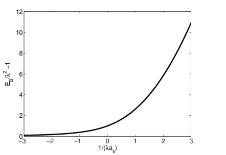
Figure 1: The quantity $E_{\text{B}}/\lambda^{2}-1$ as a function of the dimensionless parameter $\kappa=1/(\lambda a_{s})$.

The binding energy $E_{\text{B}}$ in the presence of nonzero SOC is determined by the solution of $\omega+2\mu=-E_{\text{B}}$ for the equation $\Gamma_{\text{R}}^{-1}(\omega,{\bf q}=0)=0$. From the imaginary part of $\Gamma^{-1}(\omega+i0^{+},{\bf q}=0)$, the binding energy $E_{\text{B}}$ must be larger than a threshold $E_{\text{th}}=\lambda^{2}$. The equation determining $E_{\text{B}}$ reads

$$\int_{0}^{\infty}k^{2}dk\left[\frac{1}{k^{2}}-\frac{k^{2}+E_{\text{B}}}{(k^{2}+E_{\text{B}})^{2}-4\lambda^{2}k^{2}}\right]=\frac{\pi}{2a_{s}}.$$ (26)

Completing the integrals analytically, we obtain a simple algebraic equation for $E_{\text{B}}$,

$$\frac{E_{\text{B}}-2\lambda^{2}}{\sqrt{E_{\text{B}}-\lambda^{2}}}=\frac{1}{a_{s}}.$$ (27)

We find that, for arbitrary scattering length $a_{s}$, there always exists a solution $E_{\text{B}}>\lambda^{2}$ . Therefore, the difermion bound state can form in the presence of SOC even for $a_{s}<0$ where no bound state exists in the absence of SOC.

The solution of Eq. (27) can be analytically expressed as

$$E_{\text{B}}=\lambda^{2}+\frac{1}{4}\left(\frac{1}{a_{s}}+\sqrt{\frac{1}{a_{s}^{2}}+4\lambda^{2}}\right)^{2}.$$ (28)

Therefore, the quantity $E_{\text{B}}/\lambda^{2}$ depends only on the dimensionless parameter $\kappa=1/(\lambda a_{s})$. We have

$$\frac{E_{\text{B}}}{\lambda^{2}}={\cal J}\left(\kappa\right),$$ (29)

where the function ${\cal J}(\kappa)$ is defined as

$${\cal J}(\kappa)=1+\frac{1}{4}\left(\kappa+\sqrt{\kappa^{2}+4}\right)^{2}.$$ (30)

We are interested in the case $\lambda a_{s}\rightarrow\infty$ or $\kappa=0$. This happens when $a_{s}\rightarrow\infty$ (unitary point of the Feshbach resonance) for fixed $\lambda$ or $\lambda\rightarrow\infty$ for fixed $a_{s}$. In this case, we have ${\cal J}=2$ and a very simple result

$$E_{\text{B}}(\lambda a_{s}\rightarrow\infty)=2\lambda^{2}.$$ (31)

In general, the numerical result for the quantity $E_{\text{B}}/\lambda^{2}-1={\cal J}(\kappa)-1$ is shown in Fig. 1.

Since the Hamiltonian has rotational symmetry generated by the total angular momentum ${\bf J}={\bf L}+{\bf S}$, the bound state should be a $J$ singlet. Therefore, the bound state wave function can be expressed as 3Dbound

$$\Psi({\bf r})=\psi_{0}({\bf r})|\uparrow\downarrow-\downarrow\uparrow\rangle+\psi_{1}({\bf r})|\uparrow\downarrow+\downarrow\uparrow\rangle,$$ (32)

where the spin quantization axis is chosen to be along ${\bf r}$, the relative radius of the two fermions. $\psi_{0}({\bf r})$ is an $L=0$ orbital state, while $\psi_{1}({\bf r})$ an $L=1$ orbital state. The spatial wave functions can be evaluated as 3Dbound

$$\psi_{0}({\bf r}) = \frac{e^{-br}}{r}\left(\frac{\lambda}{b}\sin{\lambda r}+\cos{\lambda r}\right)$$

$$\psi_{1}({\bf r}) = i\frac{e^{-br}}{r}\left(\left(1+\frac{1}{br}\right)\sin{\lambda r}-\frac{\lambda}{b}\cos{\lambda r}\right),$$ (33)

where $b=\sqrt{E_{\rm B}-\lambda^{2}}$. In the absence of SOC, the bound state exists only for $a_{s}>0$. We have $\psi_{1}({\bf r})=0$ and the known result $\psi_{0}({\bf r})=(1/r)e^{-r/a_{s}}$ for spin-singlet bound state. However, in the presence of SOC, the bound state is a mixture of spin-singlet and spin-triplet components. This will have a significant impact on the many-body problem, where the pair wave function possesses both spin-singlet and spin-triplet components.

III.2 Molecule effective mass

For small nonzero center-of-mass momentum ${\bf q}$, the solution for $\omega_{\bf q}$ can be written as $\omega_{\bf q}=-E_{\text{B}}+{\bf q}^{2}/(2m_{\text{B}})$, where $m_{\text{B}}$ is referred to as the effective mass of the bound state. Substituting this dispersion into the equation $\Gamma_{\text{R}}^{-1}(\omega,{\bf q})=0$ and expanding the equation to the order $O({\bf q}^{2})$, we obtain

$$\left(1-\frac{2m}{m_{\text{B}}}\right)\int_{0}^{\infty}k^{2}dk\frac{(k^{2}+E_{\text{B}})^{2}+4\lambda^{2}k^{2}}{\left[(k^{2}+E_{\text{B}})^{2}-4\lambda^{2}k^{2}\right]^{2}}$$ (34)

$$= \frac{4}{3}\int_{0}^{\infty}k^{2}dk\frac{8\lambda^{4}k^{2}}{(k^{2}+E_{\text{B}})\left[(k^{2}+E_{\text{B}})^{2}-4\lambda^{2}k^{2}\right]^{2}}.$$

Defining a new variable $x=k/\lambda$, this equation becomes

$$\left(1-\frac{2m}{m_{\text{B}}}\right)\int_{0}^{\infty}dxx^{2}\frac{(x^{2}+{\cal J})^{2}+4x^{2}}{[(x^{2}+{\cal J})^{2}-4x^{2}]^{2}}$$ (35)

$$= \frac{4}{3}\int_{0}^{\infty}dxx^{2}\frac{8x^{2}}{(x^{2}+{\cal J})[(x^{2}+{\cal J})^{2}-4x^{2}]^{2}}.$$

Completing the integrals analytically, we obtain

$$\frac{2m}{m_{\text{B}}}=\frac{7}{3}-\frac{4}{3}\left(\frac{{\cal J}-1}{{\cal J}}\right)^{3/2}-\frac{2}{{\cal J}}.$$ (36)

The effective mass therefore depends only on the combined parameter $\kappa=1/(\lambda a_{s})$. We have

$$\frac{2m}{m_{\text{B}}} = \frac{7}{3}-\frac{4}{\kappa^{2}+4+\kappa\sqrt{\kappa^{2}+4}}$$ (37)

$$- \frac{4}{3}\left(1-\frac{2}{\kappa^{2}+4+\kappa\sqrt{\kappa^{2}+4}}\right)^{3/2}.$$

The numerical result for $m_{\rm B}/2m$ is shown in Fig. 2. We find analytically that $m_{\rm B}\rightarrow 2m$ in the limit $\kappa\rightarrow+\infty$ and $m_{\rm B}\rightarrow 6m$ in the limit $\kappa\rightarrow-\infty$. For the case $\lambda a_{s}\rightarrow\infty$ or $\kappa=0$, the effective mass reads

$$\frac{m_{\text{B}}(\lambda a_{s}\rightarrow\infty)}{2m}=\frac{3(4+\sqrt{2})}{14}=1.16.$$ (38)

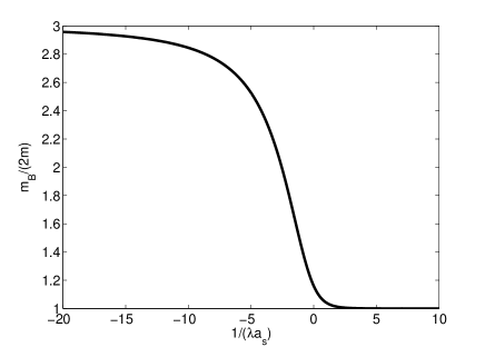
Figure 2: The molecule effective mass $m_{\text{B}}$ (divided by $2m$) as a functions of the dimensionless parameter $\kappa=1/(\lambda a_{s})$.

In summary, the difermion bound state forms in the presence of SOC for arbitrary value of s-wave scattering length $a_{s}$. The bound state possesses a non-trivial binding energy $E_{\text{B}}$ and a non-trivial effective mass $m_{\text{B}}>2m$. Such type of bound state is referred to as rashbon in the previous literatures. Due to the formation of bound state at the BCS side of the resonance ($a_{s}<0$) and the enhancement of binding energy in the presence of SOC, we expect that there will be a crossover from the BCS superfluid state to the Bose-Einstein condensation of rashbons if the spin-orbit coupling $\lambda$ can be tuned from small to large values.

IV Superfluid Ground State: Mean Field Theory

For the many-body problem, we first consider the properties of the superfluid ground state ($T=0$) in the self-consistent mean-field theory. In the superfluid ground state, the pairing field $\Phi(x)$ acquires a nonzero expectation value $\langle\Phi(x)\rangle=\Delta$, which serves as the order parameter of the superfluidity. Without loss of generality, we set $\Delta$ to be real. Then, we can express the pairing field as $\Phi(x)=\Delta+\phi(x)$, where $\phi(x)$ is the fluctuation around the mean field. The effective action ${\cal S}_{\text{eff}}[\Phi,\Phi^{*}]$ can be expanded in powers of the fluctuation,

$${\cal S}_{\text{eff}}[\Phi,\Phi^{*}]={\cal S}_{\text{eff}}^{(0)}(\Delta)+{\cal S}_{\text{eff}}^{(2)}[\phi,\phi^{*}]+\cdots,$$ (39)

where ${\cal S}_{\text{eff}}^{(0)}(\Delta)\equiv{\cal S}_{\rm eff}[\Delta,\Delta]$ is the saddle-point or mean-field effective action with the superfluid order parameter determined by the saddle-point condition $\partial{\cal S}_{\text{eff}}^{(0)}/\partial\Delta=0$.

In the mean-field approximation, the grand potential $\Omega={\cal S}_{\rm eff}[\Delta,\Delta]/(\beta V)$ can be expressed as

$$\Omega=\frac{\Delta^{2}}{U}-\frac{1}{2}\frac{1}{\beta}\sum_{n}\sum_{\bf k}\text{lndet}{\cal G}^{-1}(i\omega_{n},{\bf k}),$$ (40)

where the inverse fermion Green’s function reads

$${\cal G}^{-1}(i\omega_{n},{\bf k})=\left(\begin{array}[]{cc}i\omega_{n}-\xi_{\bf k}-\xi_{\text{so}}&i\sigma_{y}\Delta\\ -i\sigma_{y}\Delta&i\omega_{n}+\xi_{\bf k}-\xi_{\text{so}}^{*}\end{array}\right).$$ (43)

Using the formula for block matrix, we first work out the determinate and obtain

$$\text{det}{\cal G}^{-1}(i\omega_{n},{\bf k})=\left[(i\omega_{n})^{2}-(E_{\bf k}^{+})^{2}\right]\left[(i\omega_{n})^{2}-(E_{\bf k}^{-})^{2}\right],$$ (44)

where $E_{\bf k}^{\pm}=\sqrt{(\xi_{\bf k}\pm\lambda|{\bf k}|)^{2}+\Delta^{2}}$ are quasiparticle excitation spectra. Then completing the Matsubara frequency sum we obtain

$$\Omega=\frac{\Delta^{2}}{U}+\sum_{\bf k}\left[\xi_{\bf k}-{\cal W}(E_{\bf k}^{+})-{\cal W}(E_{\bf k}^{-})\right],$$ (45)

where ${\cal W}(E)=E/2+T\ln(1+e^{-E/T})$. Note that the term $\sum_{\bf k}\xi_{\bf k}\equiv\frac{1}{2}\sum_{\bf k}(\xi_{\bf k}^{+}+\xi_{\bf k}^{-})$ is added to recover the correct ground state energy for the normal state ($\Delta=0$).

IV.1 Ground-state energy

At zero temperature, the ground-state energy $E_{\rm G}\equiv\Omega(T=0)$ is $E_{\rm G}=\Delta^{2}/U+(1/2)\sum_{\bf k}(2\xi_{\bf k}-E_{\bf k}^{+}-E_{\bf k}^{-})$. Using the fact that the binding energy $E_{\rm B}$ satisfies the equation

$$\frac{1}{U}=\frac{1}{2}\sum_{\alpha=\pm}\int_{0}^{\infty}\frac{k^{2}dk}{2\pi^{2}}\frac{1}{k^{2}+2\alpha\lambda k+E_{\text{B}}},$$ (46)

we can express the ground-state energy in terms of $E_{\text{B}}$ as

$$E_{\rm G}=\frac{1}{2}\sum_{\alpha=\pm}\int_{0}^{\infty}\frac{k^{2}dk}{2\pi^{2}}\left(\frac{\Delta^{2}}{k^{2}+2\alpha\lambda k+E_{\text{B}}}-E_{k}^{\alpha}+\xi_{k}^{\alpha}\right).$$ (47)

Since the integral is convergent, we can use the trick $k^{2}\pm 2\lambda k=(k\pm\lambda)^{2}-\lambda^{2}$ and convert the integration variables to $k\pm\lambda$. Then, we obtain

$$E_{\rm G}=\int_{0}^{\infty}\frac{dk}{2\pi^{2}}(k^{2}+\lambda^{2})\left(\frac{\Delta^{2}}{k^{2}+E_{\text{B}}-\lambda^{2}}-\tilde{E}_{k}+\tilde{\xi}_{k}\right),$$ (48)

where

$$\tilde{\xi}_{k}=\epsilon_{k}-\tilde{\mu},\ \ \ \ \ \ \tilde{E}_{k}=\sqrt{\left(\epsilon_{k}-\tilde{\mu}\right)^{2}+\Delta^{2}}$$ (49)

with $\tilde{\mu}=\mu+\lambda^{2}/2$.

Using the above expression for $E_{\text{G}}$, the gap $\Delta$ and the chemical potential $\mu$ can be determined by $\partial E_{\rm G}/\partial\Delta=0$ and $\partial E_{\rm G}/\partial\mu=-n$, i.e.,

$$\int_{0}^{\infty}dk(k^{2}+\lambda^{2})\left[\frac{1}{k^{2}+E_{\text{B}}-\lambda^{2}}-\frac{1}{2\sqrt{\left(\epsilon_{k}-\tilde{\mu}\right)^{2}+\Delta^{2}}}\right]=0,$$

$$\int_{0}^{\infty}dk(k^{2}+\lambda^{2})\left[1-\frac{\epsilon_{k}-\tilde{\mu}}{\sqrt{\left(\epsilon_{k}-\tilde{\mu}\right)^{2}+\Delta^{2}}}\right]=2\pi^{2}n$$ (50)

We notice that the above expressions for the gap and number equations can be analytically evaluated using the elliptic functions, such as the analytical treatment for the gap and number equations in the absence of SOC ANAGAP .

IV.2 Fermion Green’s function

The explicit form of the fermion Green’s function ${\cal G}(i\omega_{n},{\bf k})$ can be evaluated using the formula for block matrix. In the Nambu-Gor’kov space, it takes the form

$${\cal G}(i\omega_{n},{\bf k})=\left(\begin{array}[]{cc}{\cal G}_{11}(i\omega_{n},{\bf k})&{\cal G}_{12}(i\omega_{n},{\bf k})\\ {\cal G}_{21}(i\omega_{n},{\bf k})&{\cal G}_{22}(i\omega_{n},{\bf k})\end{array}\right).$$ (53)

The matrix elements can be expressed as

$${\cal G}_{11}(i\omega_{n},{\bf k})={\cal A}_{11}(i\omega_{n},{\bf k})\hat{I}+{\cal B}_{11}(i\omega_{n},{\bf k})\hat{M},$$

$${\cal G}_{22}(i\omega_{n},{\bf k})={\cal A}_{22}(i\omega_{n},{\bf k})\hat{I}+{\cal B}_{22}(i\omega_{n},{\bf k})\hat{M}^{*},$$

$${\cal G}_{12}(i\omega_{n},{\bf k})=-i\sigma_{y}\left[{\cal A}_{12}(i\omega_{n},{\bf k})\hat{I}+{\cal B}_{12}(i\omega_{n},{\bf k})\hat{M}^{*}\right],$$

$${\cal G}_{21}(i\omega_{n},{\bf k})=i\sigma_{y}\left[{\cal A}_{21}(i\omega_{n},{\bf k})\hat{I}+{\cal B}_{21}(i\omega_{n},{\bf k})\hat{M}\right],$$ (54)

where $\hat{I}$ is the identity operator in the spin space and the operators $\hat{M}$ and $\hat{M}^{*}$ are defined as

$$\hat{M}=\frac{\mbox{\boldmath{$\sigma$}}\cdot{\bf k}}{|{\bf k}|},\ \ \ \ \hat{M}^{*} = \frac{\mbox{\boldmath{$\sigma$}}^{*}\cdot{\bf k}}{|{\bf k}|}.$$ (55)

The explicit forms of the quantities ${\cal A}_{ij}$ and ${\cal B}_{ij}$ are given by

$${\cal A}_{11}(i\omega_{n},{\bf k})=\frac{1}{2}\left[\frac{i\omega_{n}+\xi_{\bf k}^{+}}{(i\omega_{n})^{2}-(E_{\bf k}^{+})^{2}}+\frac{i\omega_{n}+\xi_{\bf k}^{-}}{(i\omega_{n})^{2}-(E_{\bf k}^{-})^{2}}\right],$$

$${\cal A}_{22}(i\omega_{n},{\bf k})=\frac{1}{2}\left[\frac{i\omega_{n}-\xi_{\bf k}^{+}}{(i\omega_{n})^{2}-(E_{\bf k}^{+})^{2}}+\frac{i\omega_{n}-\xi_{\bf k}^{-}}{(i\omega_{n})^{2}-(E_{\bf k}^{-})^{2}}\right],$$

$${\cal A}_{12}(i\omega_{n},{\bf k})=\frac{1}{2}\left[\frac{\Delta}{(i\omega_{n})^{2}-(E_{\bf k}^{+})^{2}}+\frac{\Delta}{(i\omega_{n})^{2}-(E_{\bf k}^{-})^{2}}\right],$$

$${\cal A}_{21}(i\omega_{n},{\bf k})={\cal A}_{12}(i\omega_{n},{\bf k}),$$ (56)

and

$${\cal B}_{11}(i\omega_{n},{\bf k})=\frac{1}{2}\left[\frac{i\omega_{n}+\xi_{\bf k}^{+}}{(i\omega_{n})^{2}-(E_{\bf k}^{+})^{2}}-\frac{i\omega_{n}+\xi_{\bf k}^{-}}{(i\omega_{n})^{2}-(E_{\bf k}^{-})^{2}}\right],$$

$${\cal B}_{22}(i\omega_{n},{\bf k})=-\frac{1}{2}\left[\frac{i\omega_{n}-\xi_{\bf k}^{+}}{(i\omega_{n})^{2}-(E_{\bf k}^{+})^{2}}-\frac{i\omega_{n}-\xi_{\bf k}^{-}}{(i\omega_{n})^{2}-(E_{\bf k}^{-})^{2}}\right],$$

$${\cal B}_{12}(i\omega_{n},{\bf k})=-\frac{1}{2}\left[\frac{\Delta}{(i\omega_{n})^{2}-(E_{\bf k}^{+})^{2}}-\frac{\Delta}{(i\omega_{n})^{2}-(E_{\bf k}^{-})^{2}}\right],$$

$${\cal B}_{21}(i\omega_{n},{\bf k})=-{\cal B}_{12}(i\omega_{n},{\bf k}).$$ (57)

Using the matrix elements of the Green’s function, we can calculate various quantities. First, the momentum distributions $n_{\uparrow}({\bf k})$ and $n_{\downarrow}({\bf k})$ for the two spin components can be evaluated as

$$n_{\uparrow}({\bf k})\equiv\langle\bar{\psi}_{{\bf k}\uparrow}\psi_{{\bf k}\uparrow}\rangle$$ (58)

$$= \frac{1}{\beta}\sum_{n}\left[{\cal A}_{11}(i\omega_{n},{\bf k})+\frac{k_{z}}{|{\bf k}|}{\cal B}_{11}(i\omega_{n},{\bf k})\right]e^{i\omega_{n}0^{+}},$$

$$n_{\downarrow}({\bf k})\equiv\langle\bar{\psi}_{{\bf k}\downarrow}\psi_{{\bf k}\downarrow}\rangle$$

$$= \frac{1}{\beta}\sum_{n}\left[{\cal A}_{11}(i\omega_{n},{\bf k})-\frac{k_{z}}{|{\bf k}|}{\cal B}_{11}(i\omega_{n},{\bf k})\right]e^{i\omega_{n}0^{+}}.$$

Second, the singlet and triplet pairing amplitudes can be expressed as

$$\phi_{\uparrow\downarrow}({\bf k})\equiv\langle\psi_{{\bf k}\uparrow}\psi_{-{\bf k}\downarrow}\rangle$$ (59)

$$= \frac{1}{\beta}\sum_{n}\left[-{\cal A}_{21}(i\omega_{n},{\bf k})+\frac{k_{z}}{|{\bf k}|}{\cal B}_{21}(i\omega_{n},{\bf k})\right],$$

$$\phi_{\downarrow\uparrow}({\bf k})\equiv\langle\psi_{{\bf k}\downarrow}\psi_{-{\bf k}\uparrow}\rangle$$

$$= \frac{1}{\beta}\sum_{n}\left[{\cal A}_{21}(i\omega_{n},{\bf k})+\frac{k_{z}}{|{\bf k}|}{\cal B}_{21}(i\omega_{n},{\bf k})\right],$$

$$\phi_{\uparrow\uparrow}({\bf k})\equiv\langle\psi_{{\bf k}\uparrow}\psi_{-{\bf k}\uparrow}\rangle$$

$$= -\frac{k_{x}-ik_{y}}{k}\frac{1}{\beta}\sum_{n}{\cal B}_{21}(i\omega_{n},{\bf k}),$$

$$\phi_{\downarrow\downarrow}({\bf k})\equiv\langle\psi_{{\bf k}\downarrow}\psi_{-{\bf k}\downarrow}\rangle$$

$$= \frac{k_{x}+ik_{y}}{k}\frac{1}{\beta}\sum_{n}{\cal B}_{21}(i\omega_{n},{\bf k}).$$

Third, the gap equation for $\Delta$ can be expressed as

$$\Delta=-U\frac{1}{\beta}\sum_{n}\sum_{\bf k}{\cal A}_{12}(i\omega_{n},{\bf k}).$$ (60)

IV.3 Gap and chemical potential

Using the ground state energy $E_{\rm G}$, the original forms of the gap and number equations at $T=0$ are

$$\frac{1}{U}=\frac{1}{2}\sum_{\bf k}\left(\frac{1}{2E_{\bf k}^{+}}+\frac{1}{2E_{\bf k}^{-}}\right),$$

$$n=\sum_{\bf k}\left(1-\frac{\xi_{\bf k}^{+}}{2E_{\bf k}^{+}}-\frac{\xi_{\bf k}^{-}}{2E_{\bf k}^{-}}\right).$$ (61)

The pairing gap $\Delta$ and the chemical potential $\mu$ can be numerically solved for given values of $1/(k_{\rm F}a_{s})$ and $\lambda/k_{\rm F}$. From now on, we denote the saddle point solution for the gap at zero temperature as $\Delta_{0}$. We also notice the relation

$$\frac{1}{\lambda a_{s}}=\frac{1}{k_{\text{F}}a_{s}}\left(\frac{\lambda}{k_{\rm F}}\right)^{-1}.$$ (62)

(A) Analytical Results for Large SOC. We first obtain the analytical solution at large SOC, $\lambda/k_{\rm F}\gg 1$. For large SOC, we expect $\mu<0$ and $\Delta_{0}\ll|\mu|$. Therefore, we can expand the equations in powers of $\Delta_{0}/|\mu|$ and keep only the leading order terms. The gap equation becomes

$$\frac{1}{U}=\frac{1}{2}\sum_{\alpha=\pm}\int_{0}^{\infty}\frac{k^{2}dk}{2\pi^{2}}\frac{1}{k^{2}+2\alpha\lambda k-2\mu}+O\left(\frac{\Delta_{0}^{2}}{|\mu|^{2}}\right),$$ (63)

Comparing with the two-body problem, we obtain

$$\mu\simeq-\frac{E_{\text{B}}}{2}.$$ (64)

Substituting this into the number equation, we obtain

$$n = \frac{\Delta_{0}^{2}}{8\pi^{2}}\int_{0}^{\infty}k^{2}dk\left[\frac{1}{(\xi_{k}^{+})^{2}}+\frac{1}{(\xi_{k}^{-})^{2}}\right]+O\left(\frac{\Delta_{0}^{2}}{|\mu|^{2}}\right)$$ (65)

$$\simeq \frac{\Delta_{0}^{2}}{\pi^{2}}\int_{0}^{\infty}k^{2}dk\frac{(k^{2}+E_{\text{B}})^{2}+4\lambda^{2}k^{2}}{\left[(k^{2}+E_{\text{B}})^{2}-4\lambda^{2}k^{2}\right]^{2}}.$$

We notice that this integral also appears in Eq. (25). Completing the integral analytically, we obtain

$$\Delta_{0}^{2} \simeq 4\pi\lambda n\frac{({\cal J}-1)^{3/2}}{{\cal J}}$$ (66)

$$= \frac{4\lambda\left[2\epsilon_{\rm F}({\cal J}-1)\right]^{3/2}}{3\pi{\cal J}}.$$

Therefore we have

$$\frac{\Delta_{0}}{\epsilon_{\text{F}}}\simeq\sqrt{\frac{16}{3\pi}\frac{({\cal J}-1)^{3/2}}{{\cal J}}\frac{\lambda}{k_{\text{F}}}}.$$ (67)

In the limit $\lambda a_{s}\rightarrow\infty$, we have ${\cal J}=2$ and therefore

$$\Delta_{0}^{2}(\lambda a_{s}\rightarrow\infty)\simeq 2\pi\lambda n=\frac{2\lambda(2\epsilon_{\rm F})^{3/2}}{3\pi}.$$ (68)

It can be written as another interesting form

$$\frac{\Delta_{0}(\lambda a_{s}\rightarrow\infty)}{\epsilon_{\text{F}}}\simeq\sqrt{\frac{8}{3\pi}\frac{\lambda}{k_{\text{F}}}}.$$ (69)

Therefore, for very large SOC, the gap $\Delta_{0}$ increases as $\Delta_{0}\sim\sqrt{\lambda}$.

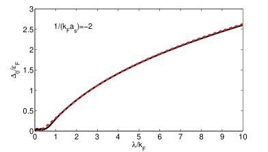
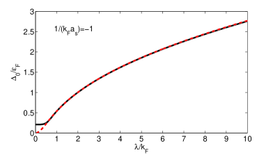
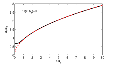
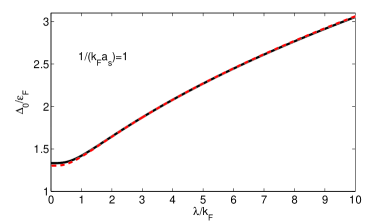
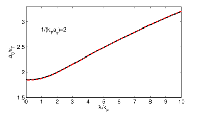
Figure 3: The pairing gap $\Delta_{0}$ (divided by $\epsilon_{\rm F}$) as a function of $\lambda/k_{\rm F}$. The red dashed line shows the analytical result (54) or (60).

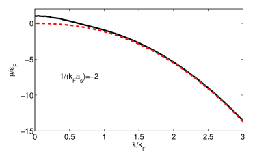
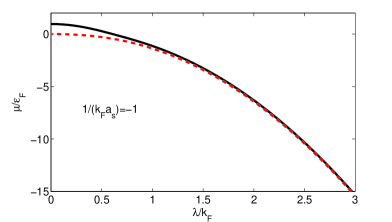
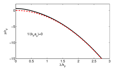
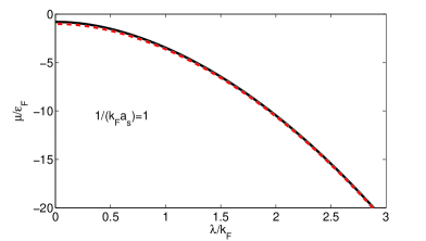
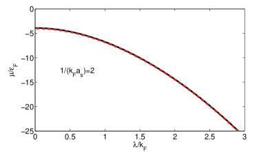
Figure 4: The chemical potential $\mu$ (divided by $\epsilon_{\rm F}$) as a function of $\lambda/k_{\rm F}$. The red dashed line shows the analytical result $\mu\simeq-\frac{E_{\rm B}}{2}$ for large SOC.

Beyond the leading order, we can write the chemical potential $\mu$ as

$$\mu=-\frac{E_{\text{B}}}{2}+\frac{\mu_{\text{B}}}{2},$$ (70)

where $\mu_{\text{B}}=2\mu+E_{\rm B}\ll E_{\rm B}$ is referred to as the effective chemical potential for bosons (rashbons). We will give an explicit expression for $\mu_{\text{B}}$ in Section V.

(B) Numerical Results. The gap and number equations (39) and (48) are equivalent. For numerical calculations, it is convenient to employ Eq. (39). If we define the following dimensionless quantities

$$g_{1}=\frac{\lambda}{k_{\rm F}},\ \ \ g_{2}=\frac{1}{k_{\rm F}a_{s}},\ \ \ x_{1}=\frac{\mu}{\epsilon_{\rm F}},\ \ \ x_{2}=\frac{\Delta_{0}}{\epsilon_{\rm F}},$$ (71)

the gap and number equations can be written as the following dimensionless form

$$\int_{0}^{\infty}dz(z^{2}+g_{1}^{2})\Bigg{[}\frac{1}{z^{2}+g_{1}^{2}{\cal J}(g_{2}/g_{1})-g_{1}^{2}}$$

$$\ \ \ \ \ \ \ \ \ \ \ \ \ \ \ \ \ \ \ \ \ \ \ -\frac{1}{\sqrt{(z^{2}-g_{1}^{2}-x_{1})^{2}+x_{2}^{2}}}\Bigg{]}=0,$$

$$\int_{0}^{\infty}dz(z^{2}+g_{1}^{2})\Bigg{[}1-\frac{z^{2}-g_{1}^{2}-x_{1}}{\sqrt{(z^{2}-g_{1}^{2}-x_{1})^{2}+x_{2}^{2}}}\Bigg{]}=\frac{2}{3}.$$ (72)

The integrals in the above equations can be analytically evaluated using elliptic functions ANAGAP . For given values of $g_{1}$ and $g_{2}$, these two equations determine $x_{1}$ and $x_{2}$.

The numerical results are shown in Fig. 3 and Fig. 4. The red dashed lines correspond to the analytical results for large SOC,

$$x_{1}=-g_{1}^{2}{\cal J}(g_{2}/g_{1}),$$

$$x_{2}=\sqrt{\frac{16g_{1}}{3\pi}\frac{[{\cal J}(g_{2}/g_{1})-1]^{3/2}}{{\cal J}(g_{2}/g_{1})}}.$$ (73)

We find that the pairing gap generally increases with increased $\lambda/k_{\rm F}$. The numerical results become in good agreement with the analytical results when $\lambda/k_{\rm F}\gtrsim 1$. Therefore, the system enters the rashbon BEC regime at $\lambda/k_{\text{F}}\sim 1$. For large positive value of $1/(k_{\rm F}a_{s})$, the analytical results are in good agreement with the numerical results even for small values of $\lambda/k_{\rm F}$. For very large $\lambda$, we find the numerical results fit very well with the following scaling behavior

$$\frac{\Delta_{0}}{\epsilon_{\rm F}}\simeq\sqrt{\frac{8}{3\pi}}\sqrt{\frac{\lambda}{k_{\rm F}}},\ \ \ \ \frac{\mu}{\epsilon_{\rm F}}\simeq-2\left(\frac{\lambda}{k_{\rm F}}\right)^{2},$$ (74)

for both negative and positive values of $1/(k_{\rm F}a_{s})$.

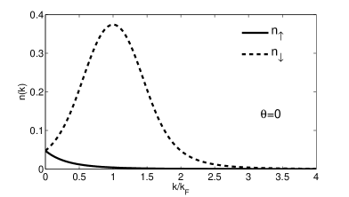
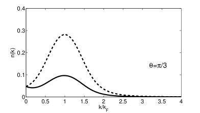
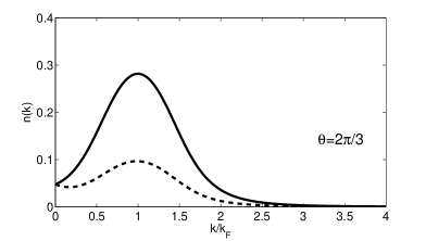
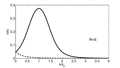
Figure 5: The fermion momentum distributions $n_{\uparrow}(k)$ and $n_{\downarrow}(k)$ for various values of the polar angle $\theta$. We set $1/(k_{\rm F}a_{s})=-1$ and $\lambda/k_{\rm F}=1$ in this calculation.

IV.4 Fermion momentum distribution

From the matrix elements of the fermion Green’s function ${\cal G}(i\omega_{n},{\bf k})$, we can obtain the momentum distributions $n_{\uparrow}({\bf k})$ and $n_{\downarrow}({\bf k})$ for the two spin components. The density of each component reads $n_{\sigma}=\sum_{\bf k}n_{\sigma}({\bf k}).$We find that even though the density of the two components are the same, $n_{\uparrow}=n_{\downarrow}$, their distributions in the momentum space are different. At zero temperature, their explicit expressions are given by

$$n_{\uparrow}(k,\theta) = \frac{1}{4}\sum_{\alpha}\left(1-\frac{\xi_{k}^{\alpha}}{E_{k}^{\alpha}}\right)+\frac{\cos\theta}{4}\sum_{\alpha}\alpha\left(1-\frac{\xi_{k}^{\alpha}}{E_{k}^{\alpha}}\right),$$

$$n_{\downarrow}(k,\theta) = \frac{1}{4}\sum_{\alpha}\left(1-\frac{\xi_{k}^{\alpha}}{E_{k}^{\alpha}}\right)-\frac{\cos\theta}{4}\sum_{\alpha}\alpha\left(1-\frac{\xi_{k}^{\alpha}}{E_{k}^{\alpha}}\right),$$ (75)

where $\theta$ is the polar angle in the momentum space. We find that $n_{\uparrow}({\bf k})=n_{\downarrow}({\bf k})$ only for $\theta=\pi/2$. We have $n_{\uparrow}({\bf k})<n_{\downarrow}({\bf k})$ for $0<\theta<\pi/2$ and $n_{\uparrow}({\bf k})>n_{\downarrow}({\bf k})$ for $\pi/2<\theta<\pi$. The reason of $n_{\uparrow}({\bf k})\neq n_{\downarrow}({\bf k})$ can be understood from the fact that the inversion symmetry ($z\rightarrow-z$) does not hold due to the presence of SOC. Meanwhile, we have $n_{\uparrow}({\bf k})=n_{\downarrow}(-{\bf k})$ due to the time reversal symmetry.

In general, with increased SOC, the distribution broadens, which indicates a BCS-BEC crossover. A numerical example for $1/(k_{\rm F}a_{s})=-1$ and $\lambda/k_{\rm F}=1$ is shown in Fig. 5. The new feature here is that the distributions generally display non-monotonous behavior due to the SOC effect. We note that the peaks in the distributions are just located at $k=\lambda$.

IV.5 Condensate density

According to Leggett’s definition FC , the condensate number of fermion pairs is given by

$$N_{0}=\frac{1}{2}\sum_{\sigma,\sigma^{\prime}=\uparrow,\downarrow}\int\int d^{3}{\bf r}d^{3}{\bf r}^{\prime}|\langle\psi_{\sigma}({\bf r})\psi_{\sigma^{\prime}}({\bf r}^{\prime})\rangle|^{2}.$$ (76)

For systems with only singlet pairing, this recovers the usual result $N_{0}=\int\int d^{3}{\bf r}d^{3}{\bf r}^{\prime}|\langle\psi_{\uparrow}({\bf r})\psi_{\downarrow}({\bf r}^{\prime})\rangle|^{2}$ FCFM . Converting this to the momentum space, we find that the condensate density $n_{0}=N_{0}/V$ is a sum of all absolute squares of the pairing amplitudes,

$$n_{0}=\frac{1}{2}\sum_{\bf k}\left[|\phi_{\uparrow\downarrow}({\bf k})|^{2}+|\phi_{\downarrow\uparrow}({\bf k})|^{2}+|\phi_{\uparrow\uparrow}({\bf k})|^{2}+|\phi_{\downarrow\downarrow}({\bf k})|^{2}\right]$$

$$=\sum_{\bf k}\left\{\left[\frac{1}{\beta}\sum_{n}{\cal A}_{21}(i\omega_{n},{\bf k})\right]^{2}+\left[\frac{1}{\beta}\sum_{n}{\cal B}_{21}(i\omega_{n},{\bf k})\right]^{2}\right\}.$$ (77)

Completing the Matsubara frequency summation and taking the zero temperature limit, we obtain the explicit expression for $T=0$,

$$n_{0} = \frac{\Delta_{0}^{2}}{16\pi^{2}}\int_{0}^{\infty}k^{2}dk\left[\frac{1}{(E_{k}^{+})^{2}}+\frac{1}{(E_{k}^{-})^{2}}\right]$$ (78)

$$= \frac{\Delta_{0}^{2}}{8\pi^{2}}\int_{0}^{\infty}dk\frac{k^{2}+\lambda^{2}}{(\epsilon_{k}-\tilde{\mu})^{2}+\Delta_{0}^{2}}.$$

Generally, we can show that $n_{0}<n/2$. For large SOC and/or attraction, we have $\Delta_{0}\ll|\mu|$. Using the number equation (39) or (48) and expanding all terms in powers of $\Delta_{0}/|\mu|$, we find that

$$n_{0}=\frac{n}{2}-O\left(\frac{\Delta_{0}^{4}}{|\mu|^{4}}\right).$$ (79)

Therefore, the condensate fraction $2N_{0}/N$ approaches unity at large SOC and/or attraction, indicating the fact that the ground state at large SOC is a Bose condensate of weakly interacting rashbons.

In general, the condensate fraction $2N_{0}/N$ can be expressed as

$$\frac{2N_{0}}{N}=\frac{3x_{2}^{2}}{4}\int_{0}^{\infty}dz\frac{z^{2}+g_{1}^{2}}{(z^{2}-g_{1}^{2}-x_{1})^{2}+x_{2}^{2}}.$$ (80)

It can be numerically obtained using the solutions of $x_{1}$ and $x_{2}$ from the gap and number equations. The numerical results are shown in Fig. 6. We find that, even for negative values of $1/(k_{\rm F}a_{s})$, the condensate fraction approaches unity around $\lambda/k_{\rm F}\sim 2$. This is consistent with the observation from the solutions of the gap and number equations that the system enters the rashbon BEC regime at $\lambda/k_{\rm F}\simeq 1$ for negative and small positive values of $1/(k_{\rm F}a_{s})$.

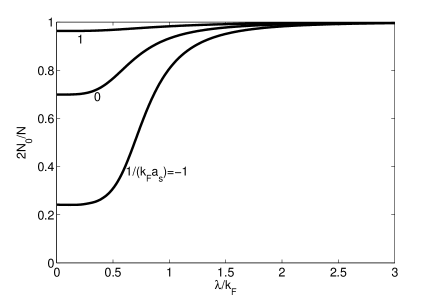
Figure 6: The condensate fraction $2N_{0}/N$ as a function of $\lambda/k_{\rm F}$ for various values of $1/(k_{\rm F}a_{s})$.

IV.6 Superfluid density

To evaluate the superfluid density $n_{s}$, we can employ the standard definition NS01 ; NS02 . When the superfluid moves with a uniform velocity $\mbox{\boldmath{$\upsilon$}}_{s}=(\upsilon_{x},\upsilon_{y},\upsilon_{z})$, the superfluid order parameter transforms like $\Phi\rightarrow\Phi e^{2i{\bf q}_{s}\cdot{\bf r}}$ and $\Phi^{*}\rightarrow\Phi^{*}e^{-2i{\bf q}_{s}\cdot{\bf r}}$, where ${\bf q}_{s}=m\mbox{\boldmath{$\upsilon$}}_{s}$ ($m=1$ in our units). The superfluid density $n_{s}$ is defined as the response of the thermodynamic potential $\Omega$ to an infinitesimal velocity velocity $\mbox{\boldmath{$\upsilon$}}_{s}$, i.e.,

$$\Omega({\bf q}_{s})=\Omega({\bf 0})+\frac{1}{2}n_{s}{\bf q}_{s}^{2}+O({\bf q}_{s}^{4}).$$ (81)

The thermodynamic potential in the presence of a velocity $\mbox{\boldmath{$\upsilon$}}_{s}$ can be evaluated by a gauge transformation for the fermion field $\psi\rightarrow\psi e^{-i{\bf q}_{s}\cdot{\bf r}}$. We have

$$\Omega({\bf q}_{s})=\frac{\Delta^{2}}{U}-\frac{1}{2}\frac{1}{\beta}\sum_{n}\sum_{\bf k}\text{lndet}{\cal G}_{s}^{-1}(i\omega_{n},{\bf k}),$$ (82)

where the inverse fermion Green function in the presence of $\mbox{\boldmath{$\upsilon$}}_{s}$ reads

$${\cal G}_{s}^{-1}(i\omega_{n},{\bf k})={\cal G}^{-1}(i\omega_{n},{\bf k})-\Sigma({\bf q}_{s}).$$ (83)

Here the velocity-dependent part $\Sigma({\bf q}_{s})$ includes three parts, $\Sigma({\bf q}_{s})=\Sigma_{1}({\bf q}_{s})+\Sigma_{2}({\bf q}_{s})+\Sigma_{3}({\bf q}_{s})$, where

$$\Sigma_{1}({\bf q}_{s})=\frac{1}{2}{\bf q}_{s}^{2}\tau_{3},$$

$$\Sigma_{2}({\bf q}_{s})={\bf k}\cdot{\bf q}_{s}\tau_{0},$$

$$\Sigma_{3}({\bf q}_{s})=\lambda(\sigma_{x}q_{x}\tau_{3}+\sigma_{y}q_{y}\tau_{0}+\sigma_{z}q_{z}\tau_{3}).$$ (84)

Here $\tau_{i}$ ($i=1,2,3$) and $\tau_{0}$ are the Pauli matrices and the identity matrix in the Nambu-Gor’kov space, respectively. We note that the term $\Sigma_{3}({\bf q}_{s})$ is purely due to the presence of SOC.

(A) Derivation of the Superfluid Density. The superfluid density $n_{s}$ can be obtained by the method of derivative expansion for $\Omega({\bf q}_{s})$, i.e.,

$$\Omega({\bf q}_{s})=\Omega({\bf 0})+\frac{1}{2}\sum_{n}\frac{1}{n}\text{Tr}\left[{\cal G}\Sigma({\bf q}_{s})\right]^{n}.$$ (85)

We find that there are four types of nonzero contributions at the order $O({\bf q}_{s}^{2})$:

$$\Omega_{1}\sim\text{Tr}({\cal G}\Sigma_{1}),\ \ \ \ \ \ \ \ \ \ \Omega_{2}\sim\text{Tr}({\cal G}\Sigma_{2}{\cal G}\Sigma_{2}),$$

$$\Omega_{3}\sim\text{Tr}({\cal G}\Sigma_{3}{\cal G}\Sigma_{3}),\ \ \ \Omega_{4}\sim\text{Tr}({\cal G}\Sigma_{2}{\cal G}\Sigma_{3}).$$ (86)

Since the superfluid state is isotropic, the superfluid density tensor should also be isotropic. We have carefully checked that all anisotropic terms vanish exactly. Completing the trace in the Nambu-Gor’kov and spin spaces, we finally obtain the following expressions for the four types of contributions:

$$\Omega_{1}=\frac{{\bf q}_{s}^{2}}{2}\frac{1}{\beta}\sum_{n}\sum_{\bf k}\frac{1}{2}\left({\cal A}_{11}e^{i\omega 0^{+}}-{\cal A}_{22}e^{-i\omega_{n}0^{+}}\right)$$

$$\Omega_{2}=\frac{{\bf q}_{s}^{2}}{2}\frac{1}{\beta}\sum_{n}\sum_{\bf k}\frac{{\bf k}^{2}}{3}\left({\cal A}_{11}^{2}+{\cal B}_{11}^{2}+{\cal A}_{22}^{2}+{\cal B}_{22}^{2}+2{\cal A}_{21}^{2}+2{\cal B}_{21}^{2}\right),$$

$$\Omega_{3}=\frac{{\bf q}_{s}^{2}}{2}\frac{1}{\beta}\sum_{n}\sum_{\bf k}\lambda^{2}\left[\left({\cal A}_{11}^{2}+{\cal A}_{22}^{2}+2{\cal A}_{21}^{2}\right)-\frac{1}{3}\left({\cal B}_{11}^{2}+{\cal B}_{22}^{2}+2{\cal B}_{21}^{2}\right)\right],$$

$$\Omega_{4}=\frac{{\bf q}_{s}^{2}}{2}\frac{1}{\beta}\sum_{n}\sum_{\bf k}\frac{4\lambda|{\bf k}|}{3}\left({\cal A}_{11}{\cal B}_{11}-{\cal A}_{22}{\cal B}_{22}+2{\cal A}_{21}{\cal B}_{21}\right).$$ (87)

Note that the first contribution is just from the total particle density $n$, $\Omega_{1}=\frac{1}{2}n{\bf q}_{s}^{2}$. Collecting all terms, the superfluid density $n_{s}$ is given by

$$n_{s}=n+\frac{1}{\beta}\sum_{n}\sum_{\bf k}\Bigg{[}\frac{{\bf k}^{2}}{3}\left({\cal A}_{11}^{2}+{\cal B}_{11}^{2}+{\cal A}_{22}^{2}+{\cal B}_{22}^{2}+2{\cal A}_{21}^{2}+2{\cal B}_{21}^{2}\right)+\frac{4\lambda|{\bf k}|}{3}\left({\cal A}_{11}{\cal B}_{11}-{\cal A}_{22}{\cal B}_{22}+2{\cal A}_{21}{\cal B}_{21}\right)$$

$$\ \ \ \ \ +\lambda^{2}\left({\cal A}_{11}^{2}+{\cal A}_{22}^{2}+2{\cal A}_{21}^{2}\right)-\frac{\lambda^{2}}{3}\left({\cal B}_{11}^{2}+{\cal B}_{22}^{2}+2{\cal B}_{21}^{2}\right)\Bigg{]}.$$ (88)

Completing the Matsubara frequency sum, we obtain the finite-temperature expression

$$n_{s} = n-\int_{0}^{\infty}\frac{k^{2}dk}{2\pi^{2}}\left[\frac{(k+\lambda)^{2}}{6}\frac{1}{2T}\frac{1}{\cosh^{2}\left(\frac{E_{k}^{+}}{2T}\right)}+\frac{(k-\lambda)^{2}}{6}\frac{1}{2T}\frac{1}{\cosh^{2}\left(\frac{E_{k}^{-}}{2T}\right)}\right]$$ (89)

$$- \frac{\lambda}{3}\int_{0}^{\infty}\frac{kdk}{2\pi^{2}}\left[\left(\xi_{k}^{+}+\frac{\Delta^{2}}{\xi_{k}}\right)\frac{1-2f(E_{k}^{+})}{E_{k}^{+}}-\left(\xi_{k}^{-}+\frac{\Delta^{2}}{\xi_{k}}\right)\frac{1-2f(E_{k}^{-})}{E_{k}^{-}}\right].$$

We have checked that this expression is consistent with the result for ordinary fermionic superfluids in the absence of SOC NS01 ; NS02 . Also, setting $\Delta=0$, we find that $n_{s}(\Delta=0)$ vanishes exactly.

We are interested in the zero temperature case. At zero temperature, the superfluid density reduces to

$$n_{s}=n-n_{\lambda},$$ (90)

where $n_{\lambda}$ is given by

$$n_{\lambda}=\frac{\lambda}{6\pi^{2}}\int_{0}^{\infty}kdk\left[\left(\xi_{k}^{+}+\frac{\Delta_{0}^{2}}{\xi_{k}}\right)\frac{1}{E_{k}^{+}}-\left(\xi_{k}^{-}+\frac{\Delta_{0}^{2}}{\xi_{k}}\right)\frac{1}{E_{k}^{-}}\right].$$ (91)

We notice that $n_{\lambda}$ vanishes in the absence of SOC and we recover the usual result $n_{s}=n$ at $T=0$ for ordinary fermionic superfluids NS01 ; NS02 . However, for nonzero SOC, $n_{\lambda}$ is always positive and we have $n_{s}(\lambda\neq 0)<n$. Therefore, the SOC leads to suppression of the superfluid density.

(B) Analytical Result for Large SOC. To understand this interesting phenomenon, we first take a look at the large SOC limit. In this case we have $\mu\simeq-E_{\text{B}}/2$ and $\Delta\ll|\mu|$. Therefore, we can expand the expression in powers of $\Delta/|\mu|$ and keep only the leading order terms. Doing so, we obtain

$$n \simeq \frac{\Delta_{0}^{2}}{8\pi^{2}}\int_{0}^{\infty}k^{2}dk\left[\frac{1}{(\xi_{k}^{+})^{2}}+\frac{1}{(\xi_{k}^{-})^{2}}\right]$$ (92)

$$\simeq \frac{\Delta_{0}^{2}}{\pi^{2}}\int_{0}^{\infty}k^{2}dk\frac{(k^{2}+E_{\text{B}})^{2}+4\lambda^{2}k^{2}}{\left[(k^{2}+E_{\text{B}})^{2}-4\lambda^{2}k^{2}\right]^{2}}$$

and

$$n_{\lambda} \simeq \frac{\lambda\Delta_{0}^{2}}{6\pi^{2}}\int_{0}^{\infty}kdk\left\{\frac{1}{\xi_{k}}\left(\frac{1}{\xi_{k}^{+}}-\frac{1}{\xi_{k}^{-}}\right)-\frac{1}{2}\left[\frac{1}{(\xi_{k}^{+})^{2}}-\frac{1}{(\xi_{k}^{-})^{2}}\right]\right\}$$ (93)

$$\simeq \frac{\Delta_{0}^{2}}{\pi^{2}}\frac{4}{3}\int_{0}^{\infty}k^{2}dk\frac{8\lambda^{4}k^{2}}{(k^{2}+E_{\text{B}})\left[(k^{2}+E_{\text{B}})^{2}-4\lambda^{2}k^{2}\right]^{2}}.$$

Comparing the above results with the equation for the molecule effective mass, we find that $n_{\lambda}/n\simeq 1-2m/m_{\text{B}}$. Therefore, at large SOC, the superfluid density is suppressed by a factor $2m/m_{\rm B}$, i.e.,

$$n_{s}\simeq\frac{2m}{m_{\text{B}}}n.$$ (94)

For $\lambda\rightarrow\infty$, using the result for $2m/m_{\rm B}$ at $\kappa=0$, we find that the ratio $n_{s}/n$ approaches a universal value,

$$\frac{n_{s}}{n}(\lambda/k_{\rm F}\rightarrow\infty)\rightarrow\frac{14}{3(4+\sqrt{2})}=0.862.$$ (95)

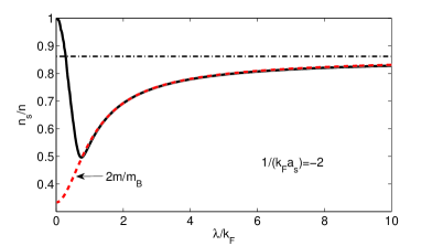
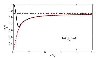
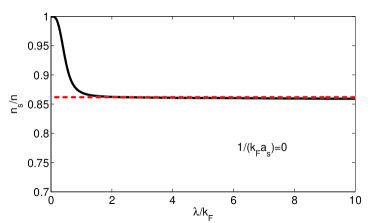
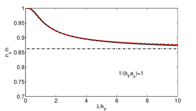
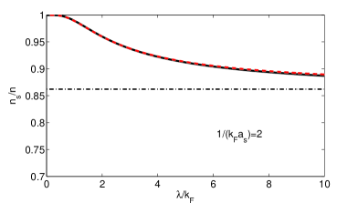
Figure 7: The superfluid density $n_{s}$ (divided by $n$) as a function of $\lambda/k_{\rm F}$ for various values of $1/(k_{\rm F}a_{s})$. The red dashed line shows the analytical result $2m/m_{\text{B}}$. The dot-dashed line corresponds to the value $0.862$ for $\lambda a_{s}\rightarrow\infty$.

To further understand this result, we consider the effective action for the phase field $\theta(x)$. To this end, we write the order parameter as $\Phi(x)=\Delta(x)e^{i\theta(x)}$. In the static limit, we can obtain the effective Hamiltonian for the phase field, $H_{\text{eff}}=(J_{s}/2)\int d^{3}{\bf r}[\nabla\theta(\bf r)]^{2}$, where the superfluid phase stiffness $J_{s}$ is related to the superfluid density $n_{s}$ by $J_{s}=n_{s}/(4m)$. Therefore, at large SOC, we have

$$J_{s}\simeq\frac{2m}{m_{\text{B}}}\frac{n}{4m}=\frac{n_{\text{B}}}{m_{\text{B}}},$$ (96)

where $n_{\text{B}}=n/2$ is the density of bosons (rashbons). This means that, at large SOC, the superfluid phase stiffness self-consistently recovers that for a rashbon gas with a non-trivial effective mass $m_{\rm B}$. We emphasize that this interesting result was first observed by us in 2D Fermi gases with Rashba spin-orbit coupling 2Dhe .

This result also indicates that the Galilean invariance, which is explicitly broken in the original fermion Hamiltonian, can be viewed as a low-energy emergent symmetry at large SOC. This is due to the fact that at large SOC the system becomes a weakly interacting Bose-Einstein condensate of non-relativistic rashbons which have a non-trivial effective mass $m_{\rm B}$. We will show this conclusion explicitly in the next section by deriving the Gross-Pitaevskii free energy for the dilute rashbon condensate at large SOC.

(C) Numerical Results. The superfluid density at zero temperature can be expressed in terms of the dimensionless parameters as

$$\frac{n_{s}}{n}=1-\frac{g_{1}}{2}\sum_{\alpha=\pm}\alpha\int_{0}^{\infty}zdz\frac{z^{2}+2\alpha g_{1}z-x_{1}+\frac{x_{2}^{2}}{z^{2}-x_{1}}}{\sqrt{(z^{2}+2\alpha g_{1}z-x_{1})^{2}+x_{2}^{2}}}.$$ (97)

It can be numerically obtained using the solutions of $x_{1}$ and $x_{2}$ from the gap and number equations.

The numerical results for $n_{s}/n$ as a function of $\lambda/k_{\rm F}$ for different values of $1/(k_{\rm F}a_{s})$ are shown in Fig. 7. For negative values or small positive values of $1/(k_{\rm F}a_{s})$, the numerical result becomes in good agreement with the analytical result $n_{s}/n\simeq 2m/m_{\text{B}}$ when $\lambda/k_{\rm F}>1$, which is consistent with the observation that the system enters the rashbon BEC regime at $\lambda/k_{\rm F}\sim 1$. For large positive values of $1/(k_{\rm F}a_{s})$ (in fact even for $1/(k_{\rm F}a_{s})=1$), the numerical results are always in good agreement with the analytical result for all values of $\lambda/k_{\rm F}$.

For both negative and positive values of $1/(k_{\rm F}a_{s})$, we find that $n/n_{s}$ approaches a universal value $0.862$ when $\lambda/k_{\rm F}\rightarrow\infty$, as indicated from the analytical observation.

IV.7 Spin susceptibility

Since the superfluid ground state exhibits spin-triplet pairing, the spin susceptibility $\chi$ can be nonzero even at zero temperature spin , in contrast to the case of vanishing SOC. The spin susceptibility is defined as the response of the system to an infinitesimal “magnetic field” ${\bf H}$, which induces an additional term $\mbox{\boldmath{$\sigma$}}\cdot{\bf H}$ in the Hamiltonian. Since the ground state is rotationally symmetric, the spin susceptibility is also isotropic. It can be evaluated by the definition

$$\Omega({\bf H})=\Omega({\bf 0})-\frac{1}{2}\chi{\bf H}^{2}+\cdots.$$ (98)

Using the derivative expansion, the spin susceptibility can be evaluated as

$$\chi = -\frac{1}{\beta}\sum_{n}\sum_{\bf k}\left({\cal A}_{11}^{2}+{\cal A}_{22}^{2}+2{\cal A}_{21}^{2}\right)$$ (99)

$$+ \frac{1}{3}\frac{1}{\beta}\sum_{n}\sum_{\bf k}\left({\cal B}_{11}^{2}+{\cal B}_{22}^{2}+2{\cal B}_{21}^{2}\right).$$

At zero temperature, the spin susceptibility reads

$$\chi=\frac{1}{6\pi^{2}\lambda}\int_{0}^{\infty}kdk\left[\left(\xi_{k}^{+}+\frac{\Delta_{0}^{2}}{\xi_{k}}\right)\frac{1}{E_{k}^{+}}-\left(\xi_{k}^{-}+\frac{\Delta_{0}^{2}}{\xi_{k}}\right)\frac{1}{E_{k}^{-}}\right].$$ (100)

This result shows explicitly that $\chi\neq 0$ for nonzero SOC. An interesting relation is that $\chi$ is proportional to the normal fluid density $n_{\lambda}=n-n_{s}$. We have

$$\chi=\frac{n-n_{s}}{\lambda^{2}}.$$ (101)

Using the result $\chi_{0}=3n/(2\epsilon_{\rm F})$ for non-interacting Fermi gases in the absence of SOC, we obtain

$$\frac{\chi}{\chi_{0}}=\frac{1}{3}\left(\frac{\lambda}{k_{\text{F}}}\right)^{-2}\left(1-\frac{n_{s}}{n}\right).$$ (102)

Therefore, at large SOC, the spin susceptibility behaves as $\chi\sim(\lambda/k_{\rm F})^{-2}$. The numerical results are shown in Fig. 8. In general, increasing the attractive strength suppresses the magnitude of $\chi$.

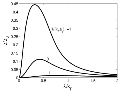
Figure 8: The spin susceptibility $\chi$ (divided by $\chi_{0}$) as a function of $\lambda/k_{\rm F}$ for various values of $1/(k_{\rm F}a_{s})$.

V Bose-Einstein Condensation of Weakly Interacting Rashbons

As we have shown in the last section, the superfluid state in the large SOC limit is a Bose-Einstein condensation of rashbons. We are interested in the interactions among the rashbons. In this section, we will derive the Gross-Pitaevskii free energy for a dilute rashbon condensate, which allow us to extract the rashbon-rashbon scattering length. Another goal of this section is to show that the Galilean invariance, which is explicitly broken in the original fermion Hamiltonian, can be effectively recovered at the boson (rashbon) level at large SOC.

To this end, we consider the mean field theory where the auxiliary boson field $\Phi(x)$ is replaced by its expectation value $\langle\Phi(x)\rangle=\Delta(x)$. In the large SOC limit $\lambda\rightarrow\infty$, the fermion chemical potential $\mu$ approaches $-E_{\text{B}}/2$. Since the pairing gap $|\Delta|\ll|\mu|$, we can expand the effective action in powers of $|\Delta|$ (as well as in powers of its space-time derivatives), which results in a Ginzburg-Landau free energy functional

$$V_{\text{GL}}[\Delta(x)]=\int dx\Bigg{[}\Delta^{\dagger}(x)\left(a\frac{\partial}{\partial\tau}-b\mbox{\boldmath{$\nabla$}}^{2}\right)\Delta(x)$$

$$\ \ \ \ \ \ \ \ \ \ \ \ \ \ \ \ \ +\ \ c|\Delta(x)|^{2}+\frac{1}{2}d|\Delta(x)|^{4}\Bigg{]}.$$ (103)

V.1 Calculation of the Ginzburg-Landau coefficients

The coefficients $c$ and $d$ of the potential terms can be obtained from the mean field thermodynamic potential $\Omega_{0}=(T/V){\cal S}_{\text{eff}}[\Delta^{\dagger},\Delta]$ which can be evaluated as

$$\Omega=-\frac{|\Delta|^{2}}{4\pi a_{s}}-\sum_{\bf k}\left(\frac{E_{\bf k}^{+}+E_{\bf k}^{-}}{2}-\xi_{\bf k}-\frac{|\Delta|^{2}}{2\epsilon_{\bf k}}\right).$$ (104)

We have

$$c=\frac{\partial\Omega}{\partial|\Delta|^{2}}\bigg{|}_{\Delta=0},\ \ \ \ d=\frac{\partial^{2}\Omega}{\partial(|\Delta|^{2})^{2}}\bigg{|}_{\Delta=0}.$$ (105)

After a simple algebra, the coefficients $\alpha$ and $\beta$ can be evaluated as

$$c=\frac{1}{4\pi}\left(\frac{-2\mu-2\lambda^{2}}{\sqrt{-2\mu-\lambda^{2}}}-\frac{1}{a_{s}}\right),$$

$$d=\frac{1}{16\pi}\frac{-2\mu+2\lambda^{2}}{(-2\mu-\lambda^{2})^{5/2}}.$$ (106)

From the expression of $c$, we find that a quantum phase transition from vacuum to Bose condensation takes place at $\mu=-E_{\rm B}/2$. Thus near the phase transition, $c$ can be simplified as

$$c\simeq-\frac{1}{8\pi}\frac{E_{\text{B}}}{\left(E_{\rm B}-\lambda^{2}\right)^{3/2}}\mu_{\text{B}},$$ (107)

where $\mu_{\text{B}}=2\mu+E_{\rm B}\ll E_{\text{B}}$ is the boson chemical potential. Further, setting $\mu=-E_{\rm B}/2$, $d$ can be reduced to

$$d\simeq\frac{1}{16\pi}\frac{E_{\rm B}+2\lambda^{2}}{(E_{\rm B}-\lambda^{2})^{5/2}}.$$ (108)

The coefficients $a$ and $b$ of the kinetic terms can be obtained from the inverse boson propagator ${\cal D}^{-1}(Q)$ with $\Delta=0$. It can be evaluated as

$${\cal D}^{-1}(Q)=\frac{1}{U}-\frac{1}{4}\sum_{\alpha,\gamma=\pm}\sum_{{\bf k}}\frac{1+\alpha\gamma{\cal T}_{\bf{kq}}}{\xi_{{\bf k}+{\bf q}/2}^{\alpha}+\xi_{{\bf k}-{\bf q}/2}^{\gamma}-i\nu_{n}}$$ (109)

In the large SOC limit, the coefficients $a$ and $b$ can be obtained by the small momentum expansion for ${\cal D}^{-1}(Q)$. We have

$${\cal D}^{-1}(Q)\simeq-a\left(i\nu_{n}+\mu_{\text{B}}-\frac{{\bf q}^{2}}{2m_{\rm B}}\right),$$ (110)

where $m_{\text{B}}$ is the rashbon effective mass determined by (28), and $a$ is given by

$$a=\frac{1}{8\pi}\frac{E_{\text{B}}}{\left(E_{\rm B}-\lambda^{2}\right)^{3/2}}.$$ (111)

We observe the relation $c={\cal D}^{-1}(0)=-a\mu_{\text{B}}$.

V.2 Gross-Pitaevskii free energy

According to the above results for the Ginzburg-Landau coefficients, if we define the new condensate wave function $\psiup(x)$ by

$$\psiup(x)=\sqrt{a}\Delta(x),$$ (112)

the Ginzgurg-Landau free energy can be reduced to the Gross-Pitaevskii free energy of a dilute Bose gas,

$$V_{\text{GP}}[\psiup(x)]=\int dx\Bigg{[}\psiup^{\dagger}(x)\left(\frac{\partial}{\partial\tau}-\frac{\mbox{\boldmath{$\nabla$}}^{2}}{2m_{\text{B}}}\right)\psiup(x)$$

$$\ \ \ \ \ \ \ \ \ \ \ \ \ \ \ \ \ -\ \ \mu_{\text{B}}|\psiup(x)|^{2}+\frac{1}{2}\frac{4\pi a_{\text{BB}}}{m_{\text{B}}}|\psiup(x)|^{4}\Bigg{]},$$ (113)

where $a_{\text{BB}}$ is the boson-boson scattering length. Its explicit expression is

$$a_{\text{BB}}=m_{\text{B}}\frac{E_{\rm B}+2\lambda^{2}}{E_{\rm B}^{2}}\sqrt{E_{\rm B}-\lambda^{2}}.$$ (114)

Note that $m=1$ in our units. For $\lambda=0$ and $a_{s}>0$, using the result $m_{\text{B}}=2$ and $E_{\rm B}=1/a_{s}^{2}$, we recover the well-known result $a_{\text{BB}}=2a_{s}$ BCSBEC3 . One remark here is that this result is the mean field result which is not exact. In the absence of SOC, exact four-body calculation shows that $a_{\text{BB}}\simeq 0.6a_{s}$ fourbody . Therefore, it is interesting to explore the exact rashbon-rashbon scattering length in the future studies. Another theoretical framework to obtain more exact $a_{\text{BB}}$ is to include the Gaussian fluctuations FL .

The Gross-Pitaevskii free energy explicitly shows that the Galilean invariance, which is explicitly broken in the original fermion Hamiltonian, can be effectively viewed as a low-energy emergent symmetry at large SOC.

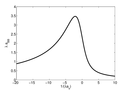
Figure 9: The molecule scattering length $a_{\text{BB}}$ (divided by $1/\lambda$) as a function of the dimensionless parameter $\kappa=1/(\lambda a_{s})$.

V.3 Rashbon-rashbon scattering length

Using the expressions for the binding energy $E_{\rm B}$ and the effective mass $m_{\text{B}}$, we obtain

$$a_{\text{BB}}=\frac{1}{\lambda}\frac{2({\cal J}+2)\sqrt{{\cal J}-1}}{{\cal J}^{2}\left[\frac{7}{3}-\frac{4}{3}\left(\frac{{\cal J}-1}{{\cal J}}\right)^{3/2}-\frac{2}{{\cal J}}\right]}.$$ (115)

We find that the quantity $\lambda a_{\text{BB}}$ depends only on the dimensionless parameter $\kappa=1/(\lambda a_{s})$. For the case $\lambda a_{s}\rightarrow\infty$ or $\kappa=0$, we have ${\cal J}=2$ and, therefore,

$$a_{\text{BB}}(\lambda a_{s}\rightarrow\infty)=\frac{1}{\lambda}\frac{3(4+\sqrt{2})}{7}=\frac{2.32}{\lambda}.$$ (116)

The numerical result for the scattering length $a_{\text{BB}}$ is shown in Fig. 9. We find that the quantity $\lambda a_{\text{BB}}$ has a maximum near the point $\kappa=0$, at $\kappa=-2.11$.

V.4 Rashbon chemical potential

For a uniform system, the expectation value of the condensate $\psiup(x)$ should be determined by minimizing the Gross-Pitaevskii free energy. We find that the minimum is given by

$$|\psiup_{0}|^{2}=\frac{\mu_{\rm B}}{g_{0}},$$ (117)

where $g_{0}=4\pi a_{\text{BB}}/m_{\text{B}}$. The total density of the bosons is $n_{\text{B}}=n/2=|\psiup_{0}|^{2}=a\Delta_{0}^{2}$. Therefore, the boson chemical potential can be given by

$$\mu_{\text{B}}=\frac{2\pi a_{\text{BB}}}{m_{\text{B}}}n.$$ (118)

For the case $\lambda a_{s}\rightarrow\infty$, using the result for $m_{\text{B}}$ and $a_{\text{BB}}$, we obtain

$$\mu_{\text{B}}(\lambda a_{s}\rightarrow\infty)=\frac{2\pi n}{\lambda}.$$ (119)

VI Gaussian Fluctuation and Collective Excitations

To study the collective excitations, we consider the fluctuations around the mean field. Making the field shift $\Phi(x)\rightarrow\Delta_{0}+\phi(x)$, we can expand the effective action ${\cal S}_{\text{eff}}$ in powers of the fluctuations. The zeroth order term ${\cal S}_{\text{eff}}^{(0)}$ is just the mean field result, and the linear terms vanish automatically guaranteed by the saddle point condition for $\Delta_{0}$. The quadratic terms, corresponding to Gaussian fluctuations, can be evaluated as

$${\cal S}_{\text{eff}}^{(2)}[\phi,\phi^{\dagger}]=\frac{1}{2}\sum_{Q}\left(\begin{array}[]{cc}\phi^{\dagger}(Q)&\phi(-Q)\end{array}\right){\bf M}(Q)\left(\begin{array}[]{cc}\phi(Q)\\ \phi^{\dagger}(-Q)\end{array}\right),$$ (123)

where the inverse boson propagator ${\bf M}$ takes the form

$${\bf M}(Q)=\left(\begin{array}[]{cc}{\bf M}_{11}(Q)&{\bf M}_{12}(Q)\\ {\bf M}_{21}(Q)&{\bf M}_{22}(Q)\end{array}\right)$$ (126)

with the relations ${\bf M}_{11}(Q)={\bf M}_{22}(-Q)$ and ${\bf M}_{12}(Q)={\bf M}_{21}(Q)$. The matrix elements of ${\bf M}(Q)$ can be expressed in terms of the fermion propagator ${\cal G}(K)$. We have

$${\bf M}_{11}(Q)=\frac{1}{U}+\frac{1}{2}\sum_{K}\text{Tr}\left[{\cal G}_{11}(K+Q)\sigma_{y}{\cal G}_{22}(K)\sigma_{y}\right],$$

$${\bf M}_{12}(Q)=-\frac{1}{2}\sum_{K}\text{Tr}\left[{\cal G}_{12}(K+Q)\sigma_{y}{\cal G}_{12}(K)\sigma_{y}\right].$$ (127)

At zero temperature, the explicit form of ${\bf M}(Q)$ can be evaluated as

$${\bf M}_{11}(Q)=\frac{1}{U}+\frac{1}{4}\sum_{\alpha,\gamma=\pm}\sum_{\bf k}\left[\frac{\left(u_{{\bf k}+{\bf q}/2}^{\alpha}\right)^{2}\left(u_{{\bf k}-{\bf q}/2}^{\gamma}\right)^{2}}{i\nu_{n}-E_{{\bf k}+{\bf q}/2}^{\alpha}-E_{{\bf k}-{\bf q}/2}^{\gamma}}-\frac{\left(v_{{\bf k}+{\bf q}/2}^{\alpha}\right)^{2}\left(v_{{\bf k}-{\bf q}/2}^{\gamma}\right)^{2}}{i\nu_{n}+E_{{\bf k}+{\bf q}/2}^{\alpha}+E_{{\bf k}-{\bf q}/2}^{\gamma}}\right]\left(1+\alpha\gamma{\cal T}_{\bf kq}\right)$$ (128)

and

$${\bf M}_{12}(Q)=\frac{1}{4}\sum_{\alpha,\gamma=\pm}\sum_{\bf k}\left[\frac{u_{{\bf k}+{\bf q}/2}^{\alpha}v_{{\bf k}+{\bf q}/2}^{\alpha}u_{{\bf k}-{\bf q}/2}^{\gamma}v_{{\bf k}-{\bf q}/2}^{\gamma}}{i\nu_{n}+E_{{\bf k}+{\bf q}/2}^{\alpha}+E_{{\bf k}-{\bf q}/2}^{\gamma}}-\frac{u_{{\bf k}+{\bf q}/2}^{\alpha}v_{{\bf k}+{\bf q}/2}^{\alpha}u_{{\bf k}-{\bf q}/2}^{\gamma}v_{{\bf k}-{\bf q}/2}^{\gamma}}{i\nu_{n}-E_{{\bf k}+{\bf q}/2}^{\alpha}-E_{{\bf k}-{\bf q}/2}^{\gamma}}\right]\left(1+\alpha\gamma{\cal T}_{\bf kq}\right).$$ (129)

Here the BCS distribution functions are defined as $(v_{\bf k}^{\alpha})^{2}=(1-\xi_{\bf k}^{\alpha}/E_{\bf k}^{\alpha})/2$ and $(u_{\bf k}^{\alpha})^{2}=(1+\xi_{\bf k}^{\alpha}/E_{\bf k}^{\alpha})/2$. In the absence of SOC, $\lambda=0$, the expressions for ${\bf M}_{11}(Q)$ and ${\bf M}_{12}(Q)$ recover the results obtained in Ref. BCSBEC3 .

VI.1 Bogoliubov excitation in the rashbon condensate

At large SOC and/or attraction, the superfluid state is a Bose-Einstein condensation of weakly interacting Bose gas. Thus, we expect that the low-energy collective excitation in this case recover the well-known Bogoliubov excitation spectrum in a weakly interacting Bose condensate Naoto . In this part, we will give an explicit proof for this.

In the large SOC and/or strong-coupling limit, the chemical potential reads $\mu\simeq-E_{\rm B}/2$ and we have $\Delta_{0}\ll|\mu|$. In this case, we can expand the matrix elements of ${\bf M}$ in powers of $\Delta_{0}/|\mu|$ and keep only the leading-order terms. Following this spirit, we obtain

$${\bf M}_{11}(Q)\simeq{\cal D}^{-1}(Q)+X\Delta_{0}^{2},$$

$${\bf M}_{12}(Q)\simeq Y\Delta_{0}^{2},$$ (130)

where the coefficients $X$ and $Y$ are given by

$$X=2Y=\frac{1}{4}\sum_{\bf k}\left[\frac{1}{(\xi_{\bf k}^{+})^{3}}+\frac{1}{(\xi_{\bf k}^{-})^{3}}\right]=2d.$$ (131)

Further, taking the small momentum expansion for ${\cal D}^{-1}(Q)$, we obtain

$${\bf M}_{11}(Q)\simeq-a\left(i\nu_{n}+\mu_{\text{B}}-\frac{{\bf q}^{2}}{2m_{\rm B}}\right)+2d\Delta_{0}^{2}.$$ (132)

Therefore, in the large SOC and/or strong coupling limit, the boson propagator ${\bf M}(Q)$ can be well approximated by

$${\bf M}_{11}(Q)\simeq a\left(-i\nu_{n}+\frac{{\bf q}^{2}}{2m_{\text{B}}}-\mu_{\text{B}}+2g_{0}|\psiup_{0}|^{2}\right)$$

$${\bf M}_{22}(Q)\simeq a\left(i\nu_{n}+\frac{{\bf q}^{2}}{2m_{\text{B}}}-\mu_{\text{B}}+2g_{0}|\psiup_{0}|^{2}\right)$$

$${\bf M}_{12}(Q)={\bf M}_{21}(Q)\simeq ag_{0}|\psiup_{0}|^{2},$$ (133)

where $g_{0}=4\pi a_{\text{BB}}/m_{\text{B}}$ and $|\psiup_{0}|^{2}=\mu_{\text{B}}/g_{0}$ is the minimum of the Gross-Pitaevskii free energy (corresponding to the saddle point $\Delta_{0}$ of the effective potential). From the Gross-Pitaevskii free energy, the boson density reads $n_{\text{B}}=n/2=|\psiup_{0}|^{2}$. Utilizing these results, we obtain

$${\bf M}(Q)\simeq a\left(\begin{array}[]{cc}-i\nu_{n}+\frac{{\bf q}^{2}}{2m_{\text{B}}}+g_{0}n_{\rm B}&g_{0}n_{\rm B}\\ g_{0}n_{\rm B}&i\nu_{n}+\frac{{\bf q}^{2}}{2m_{\text{B}}}+g_{0}n_{\rm B}\end{array}\right).$$ (136)

By taking the analytical continuation $i\nu_{n}\rightarrow\omega+i0^{+}$, the dispersion $\omega=\omega({\bf q})$ of the collective mode is obtained by solving the equation

$$\det{{\bf M}[{\bf q},\omega({\bf q})]}=0.$$ (137)

Therefore, the Goldstone mode takes a dispersion relation given by

$$\omega({\bf q})=\sqrt{\frac{{\bf q}^{2}}{2m_{\text{B}}}\left(\frac{{\bf q}^{2}}{2m_{\text{B}}}+\frac{8\pi a_{\text{BB}}n_{\text{B}}}{m_{\text{B}}}\right)}.$$ (138)

This is just the Bogoliubov excitation spectrum in a dilute Bose condensate where the bosons possess a mass $m_{\text{B}}$ and a two-body scattering length $a_{\text{BB}}$.

VI.2 Collective modes in the BCS-BEC crossover

The dispersions of the collective modes are, in principle, determined by the equation $\det{{\bf M}[{\bf q},\omega({\bf q})]}=0$. To make the result more physical, we decompose the complex fluctuation field $\phi(x)$ into its amplitude mode $\lambda(x)$ and phase mode $\theta(x)$, $\phi(x)=\lambda(x)+i\theta(x)$. Then, the fluctuation part of the effective action takes the form

$${\cal S}_{\text{eff}}^{(2)}=\frac{1}{2}\sum_{Q}\left(\begin{array}[]{cc}\lambda^{*}(Q)&\theta^{*}(Q)\end{array}\right){\bf N}(Q)\left(\begin{array}[]{c}\lambda(Q)\\ \theta(Q)\end{array}\right),$$ (139)

where the matrix ${\bf N}(Q)$ is defined as

$${\bf N}(Q)=2\left(\begin{array}[]{cc}{\bf M}_{11}^{+}+{\bf M}_{12}&i{\bf M}_{11}^{-}\\ -i{\bf M}_{11}^{-}&{\bf M}_{11}^{+}-{\bf M}_{12}\end{array}\right).$$ (140)

Here the quantities ${\bf M}_{11}^{\pm}$ are defined as

$${\bf M}_{11}^{\pm}({\bf q},\omega)=\frac{1}{2}\left[{\bf M}_{11}({\bf q},\omega)\pm{\bf M}_{11}({\bf q},-\omega)\right].$$ (141)

We notice that ${\bf M}_{11}^{+}$ and ${\bf M}_{11}^{-}$ are even and odd functions of $\omega$, respectively.

From the explicit form of ${\bf M}_{11}(Q)$, we have ${\bf M}_{11}^{-}({\bf q},0)=0$. Therefore, the amplitude and phase modes decouple completely at $\omega=0$. Furthermore, using the saddle-point condition for the order parameter $\Delta_{0}$, we find ${\bf M}_{11}^{+}({\bf 0},0)={\bf M}_{12}({\bf 0},0)$, which ensures that the phase mode at ${\bf q}=0$ is gapless, i.e., the Goldstone mode.

We now determine the velocity $c_{s}$ of the Goldstone mode, $\omega({\bf q})=c_{s}|{\bf q}|$ for $\omega,|{\bf q}|\ll\text{min}_{\bf k}\{E_{\bf k}^{\pm}\}$. For this purpose, we make a small ${\bf q}$ and $\omega$ expansion of ${\bf N}(Q)$,

$${\bf M}_{11}^{+}+{\bf M}_{12} = A+C|{\bf q}|^{2}-D\omega^{2}+\cdots,$$

$${\bf M}_{11}^{+}-{\bf M}_{12} = Q|{\bf q}|^{2}-R\omega^{2}+\cdots,$$

$${\bf M}_{11}^{-} = -B\omega+\cdots.$$ (142)

Here we note that the coefficient $Q$ is proportional to the superfluid density $n_{s}$ and the superfluid phase stiffness $J_{s}$. The explicit form of $A,\ B,\ D,\ R$ and $Q$ can be calculated as

$$A = \frac{1}{4}\sum_{\alpha=\pm}\sum_{\bf k}\frac{\Delta_{0}^{2}}{(E_{\bf k}^{\alpha})^{3}},$$

$$B = \frac{1}{8}\sum_{\alpha=\pm}\sum_{\bf k}\frac{\xi_{\bf k}^{\alpha}}{(E_{\bf k}^{\alpha})^{3}},$$

$$D = \frac{1}{16}\sum_{\alpha=\pm}\sum_{\bf k}\left[\frac{1}{(E_{\bf k}^{\alpha})^{3}}-\frac{\Delta_{0}^{2}}{(E_{\bf k}^{\alpha})^{5}}\right],$$

$$R = \frac{1}{16}\sum_{\alpha=\pm}\sum_{\bf k}\frac{1}{(E_{\bf k}^{\alpha})^{3}},$$

$$Q = \frac{J_{s}}{2\Delta_{0}^{2}}=\frac{n_{s}}{8m\Delta_{0}^{2}}.$$ (143)

The Goldstone mode velocity or the so-called sound velocity in the superfluid state is given by

$$c_{s}=\sqrt{Q\over B^{2}/A+R}.$$ (144)

The corresponding eigenvector of ${\bf N}$ is $(\lambda,\theta)=(-ic|{\bf q}|B/A,1)$, which is a pure phase mode at ${\bf q}=0$ but has an admixture of the amplitude mode controlled by $B$ at finite ${\bf q}$. Another massive mode, or the so-called Anderson-Higgs mode, has a mass gap

$$M_{g}=\sqrt{\frac{B^{2}+AR}{DR}}.$$ (145)

(A) Analytical Results for Large SOC. In the rashbon BEC limit $\lambda/k_{\text{F}}\gg 1$, we have $\mu\simeq E_{\text{B}}/2$ and $\Delta_{0}\ll|\mu|$. Therefore, the coefficients $A,\ B,\ D,\ R$ and $Q$ can be well approximated as

$$A \simeq \frac{\Delta_{0}^{2}}{4}\sum_{\alpha=\pm}\sum_{\bf k}\frac{1}{(\xi_{\bf k}^{\alpha})^{3}}=2\Delta_{0}^{2}d,$$

$$B \simeq \frac{1}{8}\sum_{\alpha=\pm}\sum_{\bf k}\frac{1}{(\xi_{\bf k}^{\alpha})^{2}}=a,$$

$$D \simeq \frac{1}{16}\sum_{\alpha=\pm}\sum_{\bf k}\frac{1}{(\xi_{\bf k}^{\alpha})^{3}}=\frac{d}{2},$$

$$R \simeq \frac{1}{16}\sum_{\alpha=\pm}\sum_{\bf k}\frac{1}{(\xi_{\bf k}^{\alpha})^{3}}=\frac{d}{2},$$

$$Q \simeq \frac{1}{2\Delta_{0}^{2}}\frac{n_{\rm B}}{m_{\text{B}}}.$$ (146)

In this case, we find that $B^{2}/A\gg R$ and therefore the amplitude and phase modes are strongly coupled.

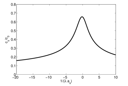
Figure 10: The sound velocity $c_{s}$ of the Goldstone mode (divided by $c_{0}$) in the RBEC regime as a function of the dimensionless parameter $\kappa=1/(\lambda a_{s})$.

The sound velocity $c_{s}$ and the mass gap $M_{g}$ read

$$c_{s}=\sqrt{AQ\over B^{2}}\simeq\sqrt{\frac{d}{a^{2}}\frac{n_{\rm B}}{m_{\rm B}}},$$

$$M_{g}=\sqrt{\frac{B^{2}}{DR}}\simeq\frac{2a}{d}.$$ (147)

Using the relation $d/a^{2}=4\pi a_{\text{BB}}/m_{\text{B}}$, the sound velocity recovers the result for a weakly interacting rashbon gas,

$$c_{s}=\sqrt{\frac{4\pi a_{\text{BB}}n_{\rm B}}{m_{\rm B}^{2}}}=\sqrt{\frac{\mu_{\rm B}}{m_{\rm B}}}.$$ (148)

Therefore, in the BEC limit, the quantity $c_{s}/c_{0}$ depends only on the dimensionless parameter $\kappa=1/(\lambda a_{s})$, where $c_{0}=\sqrt{2\pi n/\lambda}$. Using the results for $m_{\rm B}$ and $a_{\text{BB}}$, we obtain

$$c_{s}=c_{0}\sqrt{\frac{({\cal J}+2)\sqrt{{\cal J}-1}}{2{\cal J}^{2}}\left[\frac{7}{3}-\frac{4}{3}\left(\frac{{\cal J}-1}{{\cal J}}\right)^{3/2}-\frac{2}{{\cal J}}\right]}.$$ (149)

The numerical result for the quantity $c/c_{0}$ is shown in Fig. 10. We find that it has a maximum near the point $\kappa=0$, at $\kappa=-0.18$. For the case $\lambda a_{s}\rightarrow\infty$, we have

$$c_{s}(\lambda a_{s}\rightarrow\infty)=c_{0}\sqrt{\frac{7}{3(4+\sqrt{2})}}=0.66c_{0}.$$ (150)

Using the expressions for $a$ and $d$, we obtain the explicit form of the mass gap $M_{g}$,

$$M_{g}=\frac{4E_{\text{B}}(E_{\text{B}}-\lambda^{2})}{E_{\text{B}}+2\lambda^{2}}=\lambda^{2}\frac{4{\cal J}({\cal J}-1)}{{\cal J}+2}.$$ (151)

Therefore, in the BEC limit, the quantity $M_{g}/\lambda^{2}$ depends only on the dimensionless parameter $\kappa=1/(\lambda a_{s})$. The numerical result is shown in Fig. 11. We find that it is very small in the limit $\kappa\rightarrow-\infty$, and increases rapidly in the regime $\kappa>0$. For the case $\lambda a_{s}\rightarrow\infty$, we have $E_{\text{B}}=2\lambda^{2}$ and therefore

$$M_{g}(\lambda a_{s}\rightarrow\infty)=2\lambda^{2}.$$ (152)

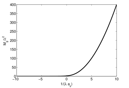
Figure 11: The mass gap $M_{g}$ of the Anderson-Higgs mode (divided by $\lambda^{2}$) in the RBEC regime as a function of the dimensionless parameter $\kappa=1/(\lambda a_{s})$.

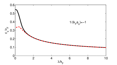
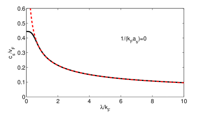
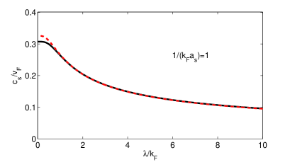
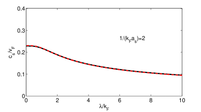
Figure 12: The velocity of the Goldstone mode (sound velocity) $c_{s}$ (divided by $\upsilon_{\rm F}$) as a function of $\lambda/k_{\rm F}$ for various values of $1/k_{\rm F}a_{s}$. The red dashed lines corresponds to the analytical result (134).

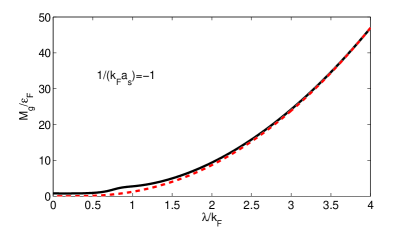
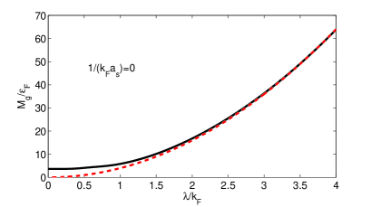
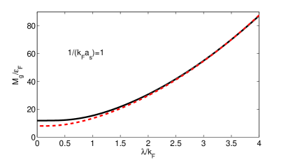
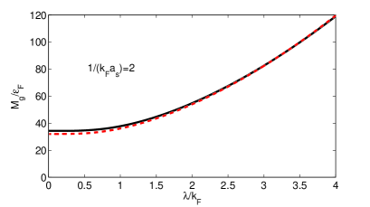
Figure 13: The mass gap $M_{g}$ of the Anderson-Higgs mode (divided by $\epsilon_{\rm F}$) as a function of $\lambda/k_{\rm F}$ for various va;lues of $1/(k_{\rm F}a_{s})$. The red dashed lines corresponds to the analytical result (136).

(B) Numerical Results. Using the same trick in Section IV, we obtain

$$A = \frac{\Delta_{0}^{2}}{4\pi^{2}}\int_{0}^{\infty}dk\frac{k^{2}+\lambda^{2}}{[(\epsilon_{k}-\tilde{\mu})^{2}+\Delta_{0}^{2}]^{3/2}}\equiv\frac{k_{\text{F}}}{2\pi^{2}}\tilde{A},$$

$$B = \frac{1}{8\pi^{2}}\int_{0}^{\infty}dk\frac{(k^{2}+\lambda^{2})(\epsilon_{k}-\tilde{\mu})}{[(\epsilon_{k}-\tilde{\mu})^{2}+\Delta_{0}^{2}]^{3/2}}\equiv\frac{1}{2\pi^{2}k_{\text{F}}}\tilde{B},$$

$$D = \frac{1}{16\pi^{2}}\int_{0}^{\infty}dk\frac{(k^{2}+\lambda^{2})(\epsilon_{k}-\tilde{\mu})^{2}}{[(\epsilon_{k}-\tilde{\mu})^{2}+\Delta_{0}^{2}]^{5/2}}\equiv\frac{1}{2\pi^{2}k_{\text{F}}^{3}}\tilde{D},$$

$$R = \frac{1}{16\pi^{2}}\int_{0}^{\infty}dk\frac{k^{2}+\lambda^{2}}{[(\epsilon_{k}-\tilde{\mu})^{2}+\Delta_{0}^{2}]^{3/2}}\equiv\frac{1}{2\pi^{2}k_{\text{F}}^{3}}\tilde{R},$$

$$Q \equiv \frac{1}{2\pi^{2}k_{\text{F}}}\tilde{Q},$$ (153)

where the dimensionless quantities $\tilde{A},\tilde{B},\tilde{D},\tilde{R}$ and $\tilde{Q}$ are defined as

$$\tilde{A}=x_{2}^{2}\int_{0}^{\infty}dz\frac{z^{2}+g_{1}^{2}}{[(z^{2}-g_{1}^{2}-x_{1})^{2}+x_{2}^{2}]^{3/2}},$$

$$\tilde{B}=\int_{0}^{\infty}dz(z^{2}+g_{1}^{2})\frac{z^{2}-g_{1}^{2}-x_{1}}{[(z^{2}-g_{1}^{2}-x_{1})^{2}+x_{2}^{2}]^{3/2}},$$

$$\tilde{D}=\int_{0}^{\infty}dz(z^{2}+g_{1}^{2})\frac{(z^{2}-g_{1}^{2}-x_{1})^{2}}{[(z^{2}-g_{1}^{2}-x_{1})^{2}+x_{2}^{2}]^{5/2}},$$

$$\tilde{R}=\int_{0}^{\infty}dz\frac{z^{2}+g_{1}^{2}}{[(z^{2}-g_{1}^{2}-x_{1})^{2}+x_{2}^{2}]^{3/2}},$$

$$\tilde{Q}=\frac{1}{3x_{2}^{2}}-\frac{g_{1}}{6x_{2}^{2}}\sum_{\alpha=\pm}\alpha\int_{0}^{\infty}zdz\frac{z^{2}+2\alpha g_{1}z-x_{1}+\frac{x_{2}^{2}}{z^{2}-x_{1}}}{\sqrt{(z^{2}+2\alpha g_{1}z-x_{1})^{2}+x_{2}^{2}}}.$$

Therefore, we have

$$\frac{c_{s}}{\upsilon_{\rm F}}=\sqrt{\tilde{Q}\over\tilde{B}^{2}/\tilde{A}+\tilde{R}}$$ (155)

and

$$\frac{M_{g}}{\epsilon_{\rm F}}=2\sqrt{\frac{\tilde{B}^{2}+\tilde{A}\tilde{R}}{\tilde{D}\tilde{R}}},$$ (156)

where $\upsilon_{\rm F}=k_{\text{F}}/m$ $(m=1)$ is the Fermi velocity for the non-interacting Fermi gas in the absence of SOC.

Using the solutions of $x_{1}$ and $x_{2}$ from the gap and number equations, we can calculate the quantity $c_{s}/\upsilon_{\rm F}$ and $M_{g}/\epsilon_{\rm F}$ for given values of $1/(k_{\rm F}a_{s})$ and $\lambda/k_{\text{F}}$. The numerical results are shown in Figs. 12 and 13. For large negative values of $1/(k_{\rm F}a_{s})$ and $\lambda/k_{\rm F}\rightarrow 0$, we recover the well-known result $c_{s}=\upsilon_{\rm F}/\sqrt{3}$ for weak coupling fermionic superfluids BCSBEC3 . For negative values or small positive values of $1/(k_{\rm F}a_{s})$, the numerical result becomes already in good agreement with the analytical results (124) and (126) at $\lambda/k_{\rm F}\sim 1$, which is consistent with the observation that the system enters the rashbon BEC regime at $\lambda/k_{\rm F}\sim 1$. For large positive values of $1/(k_{\rm F}a_{s})$, the numerical results are in good agreement with the analytical results for all values of $\lambda/k_{\rm F}$.

For very large $\lambda/k_{\rm F}$, we find that the numerical results fit very well with the following scaling behavior

$$\frac{c_{s}}{\upsilon_{\rm F}}=0.66\sqrt{\frac{2\pi}{3}}\left(\frac{\lambda}{k_{\rm F}}\right)^{-1/2},\ \ \ \ \frac{M_{g}}{\epsilon_{\rm F}}=4\left(\frac{\lambda}{k_{\rm F}}\right)^{2},$$ (157)

for both negative and positive values of $1/(k_{\rm F}a_{s})$, as indicated from the analytical observations.

VII Summary

In summary, we have presented a comprehensive study of the BCS-BEC crossover problem in 3D Fermi gases with a spherical spin-orbit coupling which can be realized by a 3D symmetrical configuration of the synthetic SU(2) gauge field. The two-body problem, the superfluid ground-state properties, and the behaviors of collective excitations are studied. Analytical results and interesting universal behaviors for various physical quantities at large SOC are obtained. We notice that there has been experimental proposal for the realization of 3D spherical spin-orbit coupling in cold fermionic atoms 3DSOC . Therefore, it is interesting to test our theoretical predictions in future experiments of cold Fermi gases with 3D spherical spin-orbit coupling.

Acknowledgments — L. He and X. -G. Huang acknowl- edge the supports from the Helmholtz International Center for FAIR within the framework of the LOEWE program (Landes- offensive zur Entwicklung Wissenschaftlich- Ökonomischer Exzellenz) launched by the State of Hesse. L. He also ac- knowledges the support from the Alexander von Humboldt Foundation.

Note Added — During the preparation of this manuscript, we became aware of the recent paper by Vyasanakere and Shenoy 3DVS , where similar results were reported.

References

- (1) D. M. Eagles, Phys. Rev. 186, 456(1969).
- (2) A. J. Leggett, in Modern trends in the theory of condensed matter, Springer-Verlag, Berlin, 1980, pp.13-27.
- (3) P. Nozieres and S. Schmitt-Rink, J. Low Temp. Phys. 59, 195(1985).
- (4) C. A. R. S a de Melo, Mohit Randeria, and Jan R. Engelbrecht, Phys. Rev. Lett. 71, 3202(1993).
- (5) Jan R. Engelbrecht, Mohit Randeria, and C. A. R. S’a de Melo, Phys. Rev. B55, 15153(1997).
- (6) Mohit Randeria, Ji-Min Duan, and Lih-Yir Shieh, Phys. Rev. Lett. 62, 981 (1989); Phys. Rev. B41, 327(1990).
- (7) Q. Chen, J. Stajic, S. Tan, and K. Levin, Phys. Rept. 412, 1(2005).
- (8) S. Giorgini, L. P. Pitaevskii, and S. Stringari, Rev. Mod. Phys. 80, 1215(2008).
- (9) V. M. Loktev, R. M. Quick, and S. G. Sharapov, Phys. Rept. 349, 1 (2001).
- (10) U. Lombardo, P. Nozieres, P. Schuck, H.-J. Schulze, and A. Sedrakian, Phys. Rev. C64, 064314(2001); X.-G. Huang, Phys. Rev. C81, 034007(2010).
- (11) L. He and P. Zhuang, Phys. Rev. D75, 096003 (2007); Phys. Rev. D76, 056003 (2007); G. Sun, L. He, and P. Zhuang, Phys. Rev. D75, 096004 (2007); L. He, Phys. Rev. D82, 096003(2010).
- (12) Y. Nishida and H. Abuki, Phys. Rev. D72, 096004(2005); H. Abuki, Nucl. Phys. A791, 117(2007); M. Kitazawa, D. H. Rischke and I. A. Shovkovy, Phys. Lett. B663, 228(2008); T. Brauner, Phys. Rev. D77, 096006(2008).
- (13) M. Greiner, C. A. Regal, D. S. Jin, Nature 426, 537(2003).
- (14) S. Jochim, M. Bartenstein, A. Altmeyer, G. Hendl, S. Riedl, C. Chin, J. Hecker Denschlag, and R. Grimm, Science 302, 2101(2003).
- (15) M. W. Zwierlein, J. R. Abo-Shaeer, A. Schirotzek, C. H. Schunck, and W. Ketterle, Nature 435, 1047(2003).
- (16) H. Hu, X. -J. Liu, and P. D. Drumond, Nat. Phys. 3, 469(2007); Y. Nishida and D. T. Son, Phys. Rev. Lett. 97, 050403(2006); M. Y. Veillette, D. E. Sheehy, and L. Radzihovsky, Phys. Rev. A75, 043614(2007).
- (17) S. Nascimb ne, N. Navon, K. Jiang, F. Chevy, and C. Salomon, Nature 463, 1057(2010); N. Navon, S. Nascimb ne, F. Chevy, and C. Salomon, Science 328, 5979(2010).
- (18) K. Osterloh, M. Baig, L. Santos, P. Zoller, and M. Lewenstein, Phys. Rev. Lett. 95, 010403(2005); J. Ruseckas, G. Juzeliunas, P. Ohberg, and M. Fleischhauer, Phys. Rev. Lett. 95, 010404(2005); T. D. Stanescu, C. Zhang, and V. Galitski , Phys. Rev. Lett. 99, 110403 (2007); X. J. Liu, M. F. Borunda, X. Liu, and J. Sinova , Phys. Rev. Lett. 102, 046402(2009); Y. J. Lin, R. L. Compton, K. Jimenez-Garcia, J. V. Porto, and I. B. Spielman, Nature 462, 628(2009); Y. J. Lin, K. Jimenez-Garcia, and I. B. Spielman, Nature 471, 83(2011).
- (19) J. D. Sau, Ra. Sensarma, S. Powell, I. B. Spielman, and S. Das Sarma, Phys. Rev. B83, 140510(R) (2011).
- (20) D. L. Campbell, G. Juzeliunas, and I. B. Spielman, Phys. Rev. A84, 025602 (2011).
- (21) G. Juzeliunas, J. Ruseckas, and J. Dalibard, Phys. Rev. A81, 053403 (2010).
- (22) J. Dalibard, F. Gerbier, G. Juzeliunas, and Patrik Ohberg, Rev. Mod. Phys. 83, 1523 (2011).
- (23) B. M. Anderson, G. Juzeliunas, I. B. Spielman, and V. M. Galitski, Phys. Rev. Lett. 108, 235301 (2012).
- (24) J. P. Vyasanakere, S. Zhang, and V. B. Shenoy, Phys. Rev. B84, 014512 (2011).
- (25) J. P. Vyasanakere and V. B. Shenoy, Phys. Rev. B83, 094515 (2011).
- (26) J. P. Vyasanakere and V. B. Shenoy, Arxiv:1108.4872.
- (27) H. Hu, L. Jiang, X.-J. Liu, and H. Pu, Phys. Rev. Lett. 107, 195304(2011); Z.-Q. Yu and H. Zhai, Phys. Rev. Lett. 107, 195305(2011).
- (28) M. Iskin and A. L. Subasi, Phys. Rev. A84, 043621(2011).
- (29) L. He and X.-G. Huang, Phys. Rev. Lett. 108, 145302 (2012).
- (30) V. P. Gusynin, D. K. Hong, and I. A. Shovkovy, Phys. Rev. D57, 5230(1998); I. A. Shovkovy and V. M. Turkowski, Phys. Lett. B367, 213(1996).
- (31) M. Gong, S. Tewari, and C. Zhang, Phys. Rev. Lett. 107, 195303(2011); M. Iskin and A. L. Subasi, Phys. Rev. Lett. 107, 050402(2011); W. Yi and G. -C. Guo, Phys. Rev. A84, 031608(R); L. Han and C. A. R. S a de Melo, Phys. Rev. A85, 011606(R) (2012); L. Dell Anna, G. Mazzarella, and L. Salasnich, Phys. Rev. A84, 033633(2011); L. Jiang, X.-J. Liu, H. Hu, and H. Pu, Phys. Rev. A84, 063618 (2011) ; K. Zhou and Z. Zhang, Phys. Rev. Lett. 108, 025301 (2012).
- (32) G. Chen, M. Gong, and C. Zhang, Phys. Rev. A85, 013601(2012).
- (33) X. Wan, A. M. Turner, A. Vishwanath, and S. Y. Savrasov, Phys. Rev. B83, 205101 (2011).
- (34) X. Cui, Phys. Rev. A85, 022705 (2012).
- (35) S. Giorgini, L. P. Pitaevskii, and S. Stringari, Rev. Mod. Phys. 80, 1215 (2008).
- (36) M. Marini, F. Pistolesi, and G. C. Strinati, Eur. Phys. J. 1, 151(1998).
- (37) A. J. Leggett, Quantum Liquids. Bose Condensation and Cooper Pairing in Condensed-Matter Systems, Oxford Universty Press, Oxford, 2006.
- (38) L. Salasnich, N. Manini, and A. Parola, Phys. Rev. A72, 023621(2005); L. Salasnich, Phys. Rev. A76, 015601(2007).
- (39) E. Taylor, A. Griffin, N. Fukushima, and Y. Ohashi, Phys. Rev. A74, 063626(2006); N. Fukushima, Y. Ohashi, E. Taylor, and A. Griffin, Phys. Rev. A75, 033609(2007).
- (40) L. He, M. Jin, and P. Zhuang, Phys. Rev. B73, 214527(2006); Phys. Rev. B74, 024516(2006); Phys. Rev. B74, 214516(2006).
- (41) L. P. Gor’kov and E. I. Rashba, Phys. Rev. Lett. 87, 037004 (2001).
- (42) D. S. Petrov, C. Salomon and G. V. Shlyapnikov, Phys. Rev. Lett. 93, 090404(2004).
- (43) H. Hu, X.-J. Liu, and P. D. Drummond, Europhys. Lett. 74, 574(2006); R. B. Diener, R. Sensarma, and M. Randeria, Phys. Rev. A77, 023626(2008).
- (44) N. Nagaosa, Quantum Field Theory in Condensed Matter Physics, Springer, 1999.
- (45) J. P. Vyasanakere and V. B. Shenoy, arXiv:1201.5332.