Fatgraph Algorithms and the Homology of the Kontsevich Complex

Abstract

Fatgraphs are multigraphs enriched with a cyclic order of the edges incident to a vertex. This paper presents algorithms to: (1) generate the set $\mathcal{R}_{g,n}$ of fatgraphs, given the genus $g$ and the number of boundary cycles $n$; (2) compute automorphisms of any given fatgraph; (3) compute the homology of the fatgraph complex $\mathcal{R}_{g,n}$. The algorithms are suitable for effective computer implementation.

In particular, this allows us to compute the rational homology of the moduli space of Riemann surfaces with marked points. We thus compute the Betti numbers of $M_{g,n}$ with $(2g+n)\leqslant 6$, corroborating known results.

1 Introduction

This paper deals with algorithms for the enumeration of fatgraphs and their automorphisms, and the computation of the homology of the complex formed by fatgraphs of a given genus $g$ and number of boundary components $n$.

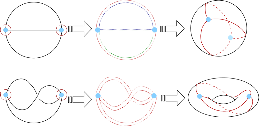
Figure 1: Thickening of a fatgraph into a Riemann surface. Left column: Starting fatgraph: the cyclic order at the vertices is given by the orientation of the ambient euclidean plane. Middle column: Thickening of the fatgraph by gluing topological disks along the boundary components. The border of a cells is drawn as a dotted line; each topological disk has been given a different color. Right column: The resulting Riemann surface with the embedded graph. Note that the two starting graphs would be isomorphic when considered as ordinary multigraphs; they are distinguished by the additional cyclic structure at the vertices.

A fatgraph is a multigraph enriched with the assignment, at each vertex $v$, of a cyclic order of the edges incident to $v$. Such graphs can be “fattened” into a smooth punctured oriented surface, by gluing polygons along the edges in such a way that two adjacent edges on the polygon boundary are consecutive in the cyclic order at the common endpoint (see Figure 1); an additional assignment of a length for each edge allows to define a conformal structure on the surface. The resulting Riemann surface is naturally marked, by choosing the marking points to be the centers of the polygons. There is thus a functorial correspondence between fatgraphs and marked Riemann surfaces; a fatgraph $G$ is said to have genus $g$ and $n$ boundary components if it corresponds to a punctured Riemann surface $S\in\mathcal{M}_{g,n}$.

In the papers [kontsevich;1993] and [kontsevich;feynman], M. Kontsevich introduced “Graph Homology” complexes that relate the stable homology groups of certain infinite-dimensional Lie algebras to various other topological objects. In particular, the “associative operad” variant of this construction results in a chain complex whose homology is isomorphic to the (co)homology of the moduli space of smooth Riemann surfaces $\mathcal{M}_{g,n}$: the graded module underlying the complex is freely generated by the set $\mathcal{R}_{g,n}$ of fatgraphs of genus $g$ and number of boundary components $n$, endowed with the differential defined by edge contraction.

The needed definitions and theorems about fatgraphs and their homology complex are briefly recalled in Section 2; the interested reader is referred to [mondello:arXiv:0705.1792v1] and [lando-zvonkin] for proofs and context.

The bulk of this paper is concerned with finding an effectively computable representation of fatgraphs (see Section 3), and presenting algorithms to:

1. compute automorphisms of any given fatgraph (Section 4);

2. generate the set $\mathcal{R}_{g,n}$ of fatgraphs, given the genus $g$ and number of boundary components $n$ (Section 5);

3. compute the homology of the fatgraph complex $\mathcal{R}_{g,n}$ (Section 6).

Note that, in contrast with other computational approaches to fatgraphs (e.g., [penner+knudsen+wiuf+andersen:2009]) which draw on the combinatorial definition of a fatgraph, our computer model of fatgraphs is directly inspired by the topological definition, and the algorithm for enumerating elements of $\mathcal{R}_{g,n}$ is likewise backed by a topological procedure.

Theorem 2.2 provides an effective way to compute the (co)homology of $\mathcal{M}_{g,n}$. The Betti numbers of $\mathcal{M}_{g,n}$ can be computed from the knowledge of the dimension of chain spaces $W_{p}$ of the fatgraph complex and the ranks of boundary operators $D_{p}$; this computation can be accomplished in the following stages:

1. Generate the basis set of $W_{*}$; by definition, the basis set is the set $\mathcal{R}_{g,n}$ of oriented fatgraphs that correspond to surfaces in $\mathcal{M}_{g,n}$.

2. Work out the differential $D\colon W_{*}\to W_{*}$ as matrices $\mathitbf{D}^{(p)}$ mapping coordinates in the fatgraph basis of $W_{p}$ into coordinates relative to the fatgraph basis of $W_{p-1}$.

3. Compute the ranks of the matrices $\mathitbf{D}^{(p)}$.

Stage I needs just the pair $g,n$ as input; its output is the set of orientable marked fatgraphs belonging in $\mathcal{R}_{g,n}$. By definition, marked fatgraphs are decorated abstract fatgraphs, and the decoration is a simple combinatorial datum (namely, a bijection of the set of boundary cycles with the set $\{1,\ldots,n\}$): therefore, the problem can be reduced to enumerating abstract fatgraphs. With a recursive algorithm, one can construct trivalent $\mathcal{M}_{g,n}$-fatgraphs from trivalent graphs in $\mathcal{M}_{g-1,n}$ and $\mathcal{M}_{g-1,n+1}$. All other graphs in $\mathcal{M}_{g,n}$ are obtained by contraction of non-loop edges.

The differential $D$ has a simple geometrical definition: $D(G)$ is a sum of graphs $G^{\prime}$, each gotten by contracting a non-loop edge of $G$. A simple implementation of Stage II would just compare each contraction of a graph with $p$ edges with any graph with $p-1$ edges, and score a $\pm 1$ (depending on the orientation) in the corresponding entry of the matrix $\mathitbf{D}^{(p)}$. However, this algorithm has quadratic complexity, and the large number of graphs involved makes it very inefficient already for $\mathcal{M}_{0,5}$. The simple observation that contraction of edges is defined on the topological fatgraph underlying a marked fatgraph allows us to apply the naive algorithm to topological fatgraphs only, which cuts complexity down by a factor $O((n!)^{2})$. The resulting matrix is then extended to marked fatgraphs by the action of graph automorphism groups on the markings of boundary cycles. This is the variant detailed in Section 6.

Stage III is conceptually the simplest: by elementary linear algebra, the Betti numbers can be computed from the rank of matrices $\mathitbf{D}^{(p)}$ and the dimension of their domain space. The computational problem of determining the rank of a matrix has been extensively studied; it should be noted, however, that this step can actually be the most computationally burdening.

It is worth mentioning that V. Godin [godin:homology] introduced a slightly different fatgraph complex, which computes the integral (co)homology of $\mathcal{M}_{g,n}$; possible adaptation of the algorithms to this complex and an outlook on the expected problems is given in Section 7.

An effective implementation (using the Python programming language [10]) of the algorithms presented here is available at http://code.google.com/p/fatghol. It has so far been used to compute the Betti numbers of $\mathcal{M}_{g,n}$ for $(2g+n)\leqslant 6$.

Results are summarized in Table 1: the values coincide with results already published in the literature. References are given in the closing Section 7, together with a discussion on the implementation performance and possible future directions for improving and extending the algorithms.

	$b_{0}$	$b_{1}$	$b_{2}$	$b_{3}$	$b_{4}$	$b_{5}$	$b_{6}$	$b_{7}$	$b_{8}$	$b_{9}$	$b_{10}$	$b_{11}$	$b_{12}$
$\mathcal{M}_{0,3}$	1
$\mathcal{M}_{0,4}$	1	2
$\mathcal{M}_{0,5}$	1	5	6
$\mathcal{M}_{0,6}$	1	9	26	24
$\mathcal{M}_{1,1}$	1
$\mathcal{M}_{1,2}$	1
$\mathcal{M}_{1,3}$	1			1
$\mathcal{M}_{1,4}$	1			4	3
$\mathcal{M}_{2,1}$	1		1
$\mathcal{M}_{2,2}$	1		2			1

Table 1: Betti numbers of $\mathcal{M}_{g,n}$ for $2g+n\leqslant 6$. For readability, null values have been omitted and the corresponding entry left blank. See Section 7 for a discussion of these results.

1.1 Notation

Algorithms are listed in pseudo-code reminiscent of the Python language syntax (see [python:reference27]); comments in the code listings are printed in italics font. The word “object” is used to denote an heterogeneous composite type in commentaries to the code listings: for our purposes, an object is just a tuple ‘”($a_{1}$, $a_{2}$, $\ldots$, $a_{N}$)”’, where each of the slots ”$a_{i}$” can be independently assigned a value; we write $X.a_{i}$ to denote the slot $a_{i}$ of object $X$. Object slots are mutable, i.e., they can be assigned different values over the course of time. Appendix B gives a complete recap of the notation used and the properties assumed of syntax, data structures, and operators.

A great deal of this paper is concerned with finding computationally-effective representations of topological objects; in general, we use boldface letters to denote the computer analog of a mathematical object. For instance, the letter $G$ always denotes a fatgraph, and $\mathitbf{G}$ its corresponding computer representation as a ”Fatgraph” object.

Finally, if $A$ is a category of which $X$, $Y$ are objects, we use Eilenberg’s notation $A(X,Y)$ for the $\operatorname{Hom}$-set, instead of the more verbose $\operatorname{Hom}_{A}(X,Y)$.

2 Fatgraphs and marked Riemann surfaces

This section recaps the main definitions and properties of fatgraphs and the relation of the fatgraph complex to the cohomology of $\mathcal{M}_{g,n}$. These results are well-known: a clear and comprehensive account is given by G. Mondello in [mondello:arXiv:0705.1792v1]; the book by Lando and Zvonkin [lando-zvonkin] provides a broad survey of the applications of fatgraphs and an introduction accessible to readers without a background in Algebraic Geometry.

“Fatgraphs” take their name from being usually depicted as graphs with thin bands as edges, instead of 1-dimensional lines; they have also been called “ribbon graphs” in algebraic geometry literature. Here, the two names will be used interchangeably.

Definition 2.1 (Geometric definition of fatgraphs).

A fatgraph is a finite CW-complex of pure dimension 1, together with an assignment, for each vertex $v$, of a cyclic ordering of the edges incident at $v$.

A morphism of fatgraphs is a cellular map $f\colon G\to G^{\prime}$ such that, for each vertex $v$ of $G^{\prime}$, the preimage $f^{-1}(V)$ of a small neighborhood $V$ of $v$ is a small neighborhood of a tree in $G$ (i.e., $f^{-1}(V)$ is a contractible connected graph).

Unless otherwise specified, we assume that all vertices of a fatgraph have valence at least 3.

If $G$ is a fatgraph, denote $V(G)$, $E(G)$ and $L(G)$ the sets of vertices, unoriented edges and oriented edges (equivalently called “legs” or “half-edges”).

Let $G$ be a fatgraph, and $G^{\prime}$ be the CW-complex obtained by contracting an edge $\alpha\in E(G)$ to a point. If $\alpha$ connects two distinct vertices (i.e., $\alpha$ is not a loop) then $G^{\prime}$ inherits a fatgraph structure from $G$: if $(\alpha<\alpha_{1}<\ldots<\alpha_{k}<\alpha)$ and $(\alpha<\alpha^{\prime}_{1}<...<\alpha^{\prime}_{h}<\alpha)$ are the cyclic orders at endpoints of $\alpha$, then the vertex formed by collapsing $\alpha$ is endowed with the cyclic order $(\alpha_{1}<\ldots<\alpha_{k}<\alpha^{\prime}_{1}<\ldots<\alpha^{\prime}_{h})$. The graph $G^{\prime}$ is said to be obtained from $G$ by contraction of $\alpha$.

Contraction morphisms play a major role in manipulation of ribbon graphs.

Lemma 2.1.

Any morphism of fatgraphs is a composition of isomorphisms and contractions of non-loop edges.

We can thus define functors $V(-)$, $E(-)$ and $L(-)$ that send morphisms of graphs to maps of their set of vertices, (unoriented) edges, and oriented edges.

The following combinatorial description of a fatgraph will also be needed:

Definition 2.2 (Combinatorial definition of fatgraph).

A fatgraph is a $4$-tuple $(L,\sigma_{0},\sigma_{1},\sigma_{2})$ comprised of a finite set $L$, together with bijective maps $\sigma_{0},\sigma_{1},\sigma_{2}\colon L\to L$ such that:

• $\sigma_{1}$ is a fixed-point free involution: $\sigma_{1}^{2}=\operatorname{id}$, and

• $\sigma_{0}\circ\sigma_{2}=\sigma_{1}$.

Lemma 2.2.

Definitions 2.1 and 2.2 are equivalent.

Any two of the maps $\sigma_{0},\sigma_{1},\sigma_{2}$ determine the third, by means of the defining relation $\sigma_{0}\circ\sigma_{2}=\sigma_{1}$; therefore, to give a ribbon graph it is sufficient to specify only two out of three maps.

In the combinatorial description, $V(G)$ is the set $L_{0}$ of orbits of $\sigma_{0}$, $E(G)$ is the set $L_{1}$ of orbits of $\sigma_{1}$, and $L(G)$ is plainly the set $L$.

There is a functorial construction to build a topological surface $S(G)$ from a fatgraph $G$; this is usually referred to as “thickening” or “fattening” in the literature.

Lemma 2.3.

There exists a functor $S$ that associates to every fatgraph $G$ a punctured Riemann surface $S(G)$, and to every morphism $f\colon G\to G^{\prime}$ a continuous map $S(f)\colon S(G)\to S(G^{\prime})$.

Denote by $B(G)$ the set $L/\sigma_{2}$ of orbits of $\sigma_{2}$: in the topological description, its elements are the support of 1-cycles in $H^{1}(G)$ that correspond under a retraction to small loops around the punctures in $S(G)$; they are called “boundary cycles” of $G$.

The assignment $G\mapsto B(G)$ extends to a functor $B(-)$; by Lemma 2.1, for any $f\colon G_{1}\to G_{2}$ the map $B(f)\colon B(G_{1})\to B(G_{2})$ is a bijection.

The correspondence between fatgraphs and Riemann surfaces allows us to give the following.

Definition 2.3.

The number of boundary cycles of a graph $G$ is given by $n=\lvert B(G)\rvert$, and is equal to the puncture number of the Riemann surface $S(G)$.

If $S(G)$ has genus $g$ and $n$ boundary cycles, then:

$$\chi(G):=\chi(S(G))=2-2g-n=2-2g-\lvert B(G)\rvert,$$ (1)

so we can define, for any fatgraph $G$, the genus $g$, as given by the relation above.

Lemma 2.4.

If $G^{\prime}$ is obtained from $G$ by contraction of a non-loop edge, then $G$ and $G^{\prime}$ share the same genus and number of boundary cycles.

Definition 2.4.

A marked fatgraph is a fatgraph $G$ endowed with a bijection $\nu:B(G)\to\{1,\ldots,n\}$. The map $\nu$ is said to be the “marking” on $G$.

A morphism $f\colon G_{1}\to G_{2}$ of marked fatgraphs must preserve the marking of boundary cycles:

$$\xymatrix{B(G_{1})&B(G_{2})\\ \{1,\ldots,n\}\ar^{f}"1,1";"1,3"\ar_{\nu_{1}}"1,1";"2,2"\ar^{\nu_{2}}"1,3";"2,2"}$$

By a slight abuse of language, we shall usually omit mention of the marking map $\nu$ and just speak of “the marked fatgraph $G$”.

2.1 Moduli spaces of marked Riemann surfaces

Fix integers $g\geqslant 0$, $n>0$ such that $2-2g-n<0$. Let $S$ be a smooth closed oriented surface of genus $g$ and $X=\{x_{1},\ldots,x_{n}\}$ a set of points of $S$.

Definition 2.5.

The Teichmüller space

$$\mathcal{T}_{g,n}:=\text{\rm Conf}(S)/\textrm{Diff}^{0}(S,n)$$

is the quotient of the set of all conformal metrics on $S$ by the set of all diffeomorphisms homotopic to the identity and fixing the $n$ marked points.

The mapping class group $\Gamma_{g,n}$ is the group of isotopy classes of self-diffeomorphisms that preserve orientation and fix marked points:

$$\Gamma_{g,n}:=\textrm{Diff}^{+}(S,n)/\textrm{Diff}^{0}(S,n).$$

The topological space $\mathcal{M}_{g,n}:=\mathcal{T}_{g,n}/\Gamma_{g,n}$ is the moduli space of (smooth) $n$-pointed algebraic curves of genus $g$. It parametrizes complex structures on $S$, up to diffeomorphisms that: (1) are homotopic to the identity mapping on $S$, (2) preserve the orientation of $S$, and (3) fix the $n$ marked points.

The Teichmüller space $\mathcal{T}_{g,n}$ is an analytic space and is homeomorphic to a convex domain in $\mathbb{C}^{3g-3+n}$. Since $\mathcal{T}_{g,n}$ is an analytic variety and $\Gamma_{g,n}$ acts discontinuously with finite stabilizers, $\mathcal{M}_{g,n}$ inherits a structure of analytic orbifold of complex dimension $3g-3+n$.

Since $\mathcal{T}_{g,n}$ is contractible, its equivariant (co)homology with rational coefficients is isomorphic to the rational (co)homology of $\mathcal{M}_{g,n}$ (see [8, VII.7.7]).

2.2 The fatgraph cellularization of the moduli spaces of marked Riemann surfaces

An embedding of a fatgraph $G$ is an injective continuous map $\iota\colon G\to S$, that is, a homeomorphism of $G$ onto $\iota(G)\subseteq S$, such that the orientation on $S$ induces the cyclic order at the vertices of $\iota(G)$.

Definition 2.6.

An embedded fatgraph is a fatgraph $G$ endowed with a homeomorphism ${\tilde{\iota}}$ between $S(G)$ and the ambient surface $S$, modulo the action of $\textrm{Diff}^{0}(S)$.

There is an obvious action of $\Gamma_{g,n}$ on the set $\mathscr{\widetilde{R}}_{g,n}$ of fatgraphs embedded into $n$-marked Riemann surfaces of genus $g$.

If confusion is likely to arise, we shall speak of abstract fatgraphs, to mean the topological and combinatorial objects defined in Definition 2.1, as opposed to embedded fatgraphs as in Definition 2.6 above.

Definition 2.7.

A metric $\ell$ on a fatgraph $G$ is an assignment of a real positive number $\ell_{\alpha}$ for each edge $\alpha\in E(G)$.

Given a metric $\ell$ on a fatgraph $G$, the “thickening” construction for fatgraphs can be extended to endow the surface $S(G)$ with a conformal structure dependent on $\ell$. Conversely, a theorem due to Jenkins and Strebel guarantees that a metric can be defined on each fatgraph embedded in a surface $S$, depending uniquely on the conformal structure on $S$.

Let $G$ be a fatgraph (embedded or abstract) of genus $g$ with $n$ marked boundary components. The set $\Delta(G)=\{(G,\ell)\}$ of metrics on $G$ has an obvious structure of topological cell; now glue these cells by stipulating that $\Delta(G^{\prime})$ is the face $\ell_{\alpha}=0$ of $\Delta(G)$ when $G^{\prime}$ is obtained from $G$ by contraction of the edge $\alpha$. The topological spaces obtained by this gluing instructions are denoted $\mathcal{T}^{\text{comb}}_{g,n}$ (when using embedded fatgraphs), or $\mathcal{M}^{\text{comb}}_{g,n}$ (when using abstract fatgraphs). The following theorem clarifies their relation to the Teichmüller and the moduli space; details can be found, e.g., in [mondello:arXiv:0705.1792v1, Section 4.1].

Theorem 2.1.

The thickening construction induces orbifold isomorphisms:

$$\mathcal{T}_{g,n}\times\mathbb{R}^{n}\simeq\mathcal{T}^{\text{comb}}_{g,n},\qquad\mathcal{M}_{g,n}\times\mathbb{R}^{n}\simeq\mathcal{M}^{\text{comb}}_{g,n},$$

Call $M(G)$ the cell in $\mathcal{M}^{\text{comb}}_{g,n}$ corresponding to an abstract fatgraph $G$, and $T(\tilde{G})$ the cell in $\mathcal{T}^{\text{comb}}_{g,n}$ corresponding to an embedded fatgraph $\tilde{G}$.

The functorial action of $\Gamma_{g,n}$ on $\mathscr{\widetilde{R}}_{g,n}$ induces an action on $\mathcal{T}^{\text{comb}}_{g,n}$, which permutes cells $T({\tilde{G}})$ by PL isomorphisms.

Lemma 2.5.

$\mathcal{M}^{\text{comb}}_{g,n}$ is the quotient space of $\mathcal{T}^{\text{comb}}_{g,n}$ by the cellular action of the mapping class group $\Gamma_{g,n}$; the projection homomorphism commutes with the isomorphisms in Theorem 2.1.

Lemma 2.6.

The isotropy group $\Gamma_{{\tilde{G}}}$ of the cell $T({\tilde{G}})\hookrightarrow\mathcal{T}^{\text{comb}}_{g,n}$ is (isomorphic to) the automorphism group $\operatorname{Aut}G$ of the abstract fatgraph $G$ underlying ${\tilde{G}}$.

The action of $\Gamma_{g,n}$ commutes with the face operators, so $M(G)$ is a face of $M(G^{\prime})$ iff $G^{\prime}$ is obtained from $G$ by contraction of a non-loop edge.

2.3 Equivariant homology of $\mathcal{T}_{g,n}$ and the complex of fatgraphs

Definition 2.8.

An orientation of a fatgraph $G$ is an orientation of the vector space $\mathbb{Q}E(G)$, that is, the choice of an order of the edges of $G$, up to even permutations.

Giving an orientation on $G$ (resp. ${\tilde{G}}$) is the same as orienting the simplex $\Delta(G)$ (resp. $T({\tilde{G}})$).

If $G$ is a fatgraph with $p$ edges, let $W_{G}:=\bigwedge^{p}\mathbb{Q}E(G)$ be the 1-dimensional vector space generated by the wedge products $\alpha_{1}\land\ldots\land\alpha_{p}$ of edges of $G$. Every $f\in\operatorname{Aut}G$ induces a map $f:E(G)\to E(G)$ on the edges and thus a map $f_{*}:\alpha_{1}\land\ldots\land\alpha_{p}\mapsto f(\alpha_{1})\land\ldots\land f(\alpha_{p})$. Trivially, $f_{*}(\alpha_{1}\land\ldots\land\alpha_{p})=\pm\alpha_{1}\land\ldots\land\alpha_{p}$, depending on whether $f$ preserves or reverses the orientation of $G$.

Definition 2.9.

A fatgraph $G$ is orientable iff it has no orientation-reversing automorphisms.

Form a differential complex of orientable fatgraphs as follows.

Definition 2.10.

The complex $(W_{*},D)$ of orientable fatgraphs is defined by:

• $W_{p}:=\bigoplus_{G}W_{G}$, where $G$ runs over orientable fatgraphs with $(2g+n-1+p)$ edges;

• $D:=\sum_{1}^{p}(-1)^{i}d_{i}$, where $d_{i}\colon W_{p}\to W_{p-1}$ is given by:

  $$d_{i}(\alpha_{1}\land\ldots\land\alpha_{p}):=\begin{cases}\alpha_{1}\land\ldots\land\widehat{\,\alpha_{i}\,}\land\ldots\land\alpha_{p}&\parbox[t]{100.00015pt}{if $\alpha_{i}$ is not a loop and $G/\alpha_{i}$ is orientable,}\\ 0&\text{otherwise.}\end{cases}$$

Every oriented fatgraph $(G,\omega)$ defines an element $\omega_{G}\in W_{G}$ by taking the wedge product of edges of $G$ in the order given by $\omega$; conversely, any $\alpha_{1}\land\ldots\land\alpha_{p}\in W_{G}$ defines an orientation on $G$ by setting $\omega:=\alpha_{1}<\ldots<\alpha_{p}$.

Theorem 2.2.

The $\Gamma_{g,n}$-equivariant homology of $\mathcal{T}_{g,n}$ with rational coefficients is computed by the complex of oriented fatgraphs $(W_{*},D)$, i.e., there exists an isomorphism:

$$H^{\Gamma_{g,n}}_{*}(\mathcal{T}_{g,n},\mathbb{Q})\cong H_{*}(W_{*},D).$$

Proof.

The genus and number of boundary cycles will be fixed throughout, so for brevity, set $\Gamma:=\Gamma_{g,n}$, $\mathcal{T}:=\mathcal{T}_{g,n}$ and $\mathcal{T}^{\text{comb}}:=\mathcal{T}^{\text{comb}}_{g,n}$.

By Theorem 2.1, we have:

$$H^{\Gamma}_{*}(\mathcal{T},\mathbb{Q})=H^{\Gamma}_{*}(\mathcal{T}^{\text{comb}},\mathbb{Q}).$$

Recall that $H^{\Gamma}_{*}(\mathcal{T}^{\text{comb}},\mathbb{Q})$ can be defined as the homology of the double complex $P_{*}\otimes C_{*}(\mathcal{T}^{\text{comb}},\mathbb{Q})$, where $P_{*}$ is any projective resolution of $\mathbb{Q}$ over $\mathbb{Q}[\Gamma]$. The spectral sequence $E^{1}_{pq}:=H_{q}(P_{*}\otimes_{\Gamma}C_{p})=H_{q}(\Gamma,C_{p})$ abuts to $H^{\Gamma}_{p+q}(\mathcal{T}^{\text{comb}})$ (see [8, VII.5 and VII.7]).

The space $\mathcal{T}^{\text{comb}}_{g,n}$ has, by definition, an equivariant cellularization with cells indexed by embedded fatgraphs of genus $g$ with $n$ marked boundary components. Let $R_{p}$ be a set of representatives for the orbits of $p$-cells under the action of $\Gamma$. By Lemma 2.5, $R_{p}$ is in bijective correspondence with the set of abstract fatgraphs having $p$ edges, and the orientation of a cell translates directly to an orientation of the corresponding graph. For each geometric simplex $T({\tilde{G}})\subseteq\mathcal{T}^{\text{comb}}$, let $\Gamma_{\tilde{G}}$ be its isotropy group, and let $\mathbb{Q}{\tilde{G}}$ be the $\Gamma_{\tilde{G}}$-module consisting of the $\mathbb{Q}$-vector space generated by an element $\Delta$ on which $\Gamma_{\tilde{G}}$ acts by the orientation character: $\tau\cdot\Delta=\pm\Delta$ depending on whether $\tau$ preserves or reverses the orientation of the cell $T({\tilde{G}})$. By Lemma 2.6, there is an isomorphism between $\Gamma_{\tilde{G}}$ and $\operatorname{Aut}G$; if $\tau\in\Gamma_{\tilde{G}}$ reverses (resp. preserves) orientation of $T({\tilde{G}})$, then the corresponding $f\in\operatorname{Aut}G$ reverses (resp. preserves) orientation on $G$. Therefore, $\mathbb{Q}{\tilde{G}}$ and $W_{G}$ are isomorphic as $\operatorname{Aut}G=\Gamma_{T{\tilde{G}}}$ modules.

Following [8, p. 173], let us decompose (as a $\Gamma$-module)

$$C_{*}(\mathcal{T}^{\text{comb}},\mathbb{Q})=\bigoplus_{G\in R_{p}}W_{G};$$

then, by Shapiro’s lemma [8, III.6.2], we have:

$$H_{q}(\Gamma,C_{p})\cong\bigoplus_{G\in R_{p}}H_{q}(\Gamma_{\tilde{G}},\mathbb{Q}{\tilde{G}})\cong\bigoplus_{G\in R_{p}}H_{q}(\operatorname{Aut}G,W_{G}).$$

Since $\operatorname{Aut}G$ is finite and we take rational coefficients, then $H_{q}(\operatorname{Aut}G,W_{G})=0$ if $q>0$ [8, III.10.2]. On the other hand, if $G$ is orientable then $\operatorname{Aut}G$ acts trivially on $W_{G}$, so:

$$H_{0}(\operatorname{Aut}G,W_{G})=\begin{cases}0&\text{if $G$ has an orientation-reversing automorphism,}\\ W_{G}&\text{if $G$ has \emph{no} orientation-reversing automorphisms.}\end{cases}$$

Let $R^{\prime}_{p}$ be the collection of all orientable fatgraphs with $p$ edges. Substituting back into the spectral sequence, we see that only one column survives:

$$E^{1}_{p,0} =\bigoplus_{G\in R^{\prime}_{p}}W_{G}=W_{p},$$ (2)

$$E^{1}_{p,q} =0 q>0$$ for all , (3)

In other words, $E^{1}_{pq}$ reduces to the complex $(E^{1}_{*,0},d^{1})$.

Finally, we show that the differential $d^{1}\colon E^{1}_{p,0}\to E^{1}_{p-1,0}$ corresponds to the differential $D\colon W_{p}\to W_{p-1}$ under the isomorphism formula (2); this will end the proof. Indeed, we shall prove commutativity of the following diagram at the chain level:

$$\xymatrix{P_{*}\otimes W_{p}&\bigoplus_{G\in R^{\prime}_{p}}P_{*}\otimes W_{G}\bigoplus_{G^{\prime}\in R^{\prime}_{p-1}}P_{*}\otimes W_{G^{\prime}}P_{*}\otimes W_{p-1}\\ P_{*}\otimes C_{p}(\mathcal{T}^{\text{comb}},\mathbb{Q})P_{*}\otimes C_{p-1}(\mathcal{T}^{\text{comb}},\mathbb{Q})\ar^{\operatorname{id}_{P}\otimes D}"1,2";"1,3"\ar_{\operatorname{id}_{P}\otimes\partial}"2,2";"2,3"\ar_{\theta_{p}}"1,2";"2,2"\ar^{\theta_{p-1}}"1,3";"2,3"\ar@{=}"1,1";"1,2"\ar@{=}"1,3";"1,4"}$$ (4)

which implies commutativity at the homology level:

$$\xymatrix{\bigoplus_{G\in R^{\prime}_{p}}H_{0}(\operatorname{Aut}G,W_{G})&\bigoplus_{G^{\prime}\in R^{\prime}_{p-1}}H_{0}(\operatorname{Aut}G^{\prime},W_{G^{\prime}})\\ H_{0}(\Gamma,C_{p}(\mathcal{T}^{\text{comb}},\mathbb{Q}))H_{0}(\Gamma,C_{p-1}(\mathcal{T}^{\text{comb}},\mathbb{Q}))\ar^{D}"1,1";"1,2"\ar_{d^{1}=H_{0}(\Gamma,\partial)}"2,1";"2,2"\ar_{\cong}"1,1";"2,1"\ar^{\cong}"1,2";"2,2"}$$

whence the conclusion $E^{1}_{*,0}\cong(W_{*},D)$.

The vertical maps $\theta_{p}$, $\theta_{p-1}$ in (4) are the chain isomorphisms underlying the $\Gamma$-module decomposition $C_{p}(\mathcal{T}^{\text{comb}},\mathbb{Q})\cong\bigoplus_{G\in R_{p}}W_{G}$. Taking the boundary of a cell $T({\tilde{G}})\subseteq\mathcal{T}^{\text{comb}}$ commutes with the $\Gamma$-action: $\partial T(\tau\cdot{\tilde{G}})=\tau\cdot\partial T({\tilde{G}})$. Furthermore, $T({\tilde{G}}^{\prime})$ is a cell in $\partial T({\tilde{G}})$ iff ${\tilde{G}}^{\prime}$ is obtained from ${\tilde{G}}$ by contraction of an edge; but ${\tilde{G}}^{\prime}$ is a contraction of ${\tilde{G}}$ iff the underlying abstract fatgraphs $G^{\prime}$ and $G$ stand in the same relation. Thus, the $\Gamma$-complexes $(C_{*},\partial)$ and $(W_{*},D)$ are isomorphic by $\theta_{*}$, so diagram (4) commutes, as was to be proved. ∎

3 Computer representation of Fatgraphs

Although the combinatorial definition of a fatgraph (cf. Lemma 2.2) lends itself to a computer representation as a triple of permutations —as used, e.g., in [penner+knudsen+wiuf+andersen:2009, Section 2.4]—, the functions that are needed by the generation algorithms (see Section 5) are rather topological in nature and thus suggest an approach more directly related to the concrete realization of a fatgraph.

Definition 3.1.

A ”Fatgraph” object $\mathitbf{G}$ is comprised of the following data:

• A list ”$\mathitbf{G}$.vertices” of ”Vertex” objects.

• A list ”$\mathitbf{G}$.edges” of ”Edge” objects.

• A set ”$\mathitbf{G}$.boundary_cycles” of ”BoundaryCycle” objects.

• An orientation ”$\mathitbf{G}$.orient”.

The exact definition of the constituents of a ”Fatgraph” object is the subject of the following sections; informally, let us say that a ”Vertex” is a cyclic list of edges and that an ”Edge” is a pair of vertices and incidence positions. A precise statement about the correspondence of abstract fatgraphs and ”Fatgraph” objects is made in Section 3.5.

There is some redundancy in the data comprising a ”Fatgraph” object: some of these data are inter-dependent and cannot be specified arbitrarily. Actually, all data comprising a ”Fatgraph” object can be computed from the vertex list alone, as the following sections show.

In what follows, the letters $l$, $m$ and $n$ shall denote the number of vertices, edges and boundary cycles:

• ”$l$ == $\lvert V(G)\rvert$ == size($\mathitbf{G}$.vertices)”,

• ”$m$ == $\lvert E(G)\rvert$ == size($\mathitbf{G}$.edges)”,

• ”$n$ == $\lvert B(G)\rvert$ == size($\mathitbf{G}$.boundary_cycles)”.

For integers $\alpha$ and $k$, we use $(\alpha\%k)$ to denote the smallest non-negative representative of $\alpha\mod k\;$.

3.1 Vertices

We can represent a fatgraph vertex by assigning labels to all fatgraph vertices and mapping a vertex to the cyclically-invariant list of labels of incident edges. Figure 2 gives an illustration.

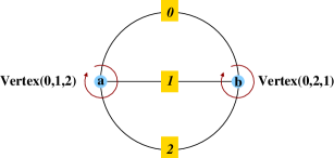
Figure 2: Representation of vertices as (cyclic) lists of edge labels; vertices are identified by lowercase Latin letters; edge labels are depicted as roman numerals on a yellow square background, sitting over the edge they label. The representation of a vertex as a list is implicitly ciliated: here we use the convention that the edge closest to the tail of the arrow is the ciliated one.

Definition 3.2.

A vertex together with a choice of an attached edge is called a ciliated vertex. The chosen edge is called the cilium.

Definition 3.3.

If $v$ is a ciliated vertex and $e$ is a half-edge attached to it, define the attachment index of $e$ at $v$ as the index of edge $e$ relative to the cilium at $v$: if $\alpha$ is the attachment index of $e$ at $v$, then $\sigma_{0}^{\alpha}$ takes the cilium at $v$ onto $e$.

The attachment index at a vertex is unambiguously defined for all edges which are not loops; the two half-edges comprising a loop have distinct attachment indices. For brevity, in the following we shall slightly abuse the definition and speak of the attachment index of an edge at a vertex.

Definition 3.4.

A ”Vertex” object ”$\mathitbf{v}$ == Vertex($e_{1}$, $\ldots$, $e_{z}$)” is a list of the labels $e_{1}$, …, $e_{z}$ of attached edges.

Two ”Vertex” objects are considered equal if one is equal (as a sequence) to the other rotated by a certain amount.

Note that the definition of ”Vertex” objects as plain lists corresponds to ciliated vertices in a fatgraph. In order to implement the cyclic behavior of fatgraph vertices, the requirement on equality must be imposed; equality of ”Vertex” objects can be tested by an algorithm of quadratic complexity in the vertex valence.

If $\mathitbf{v}$ is a vertex object, let us denote ”num_loops($\mathitbf{v}$)” the number of loops attached to $\mathitbf{v}$; it is a vertex invariant and will be used in the computation of fatgraph isomorphisms. Implementations of ”num_loops” need only count the number of repeated edge labels in the list defining the ”Vertex” object $\mathitbf{v}$.

3.2 Edges

Definition 3.5.

An ”Edge” object $\mathitbf{e}$ is an unordered pair of endpoints, so defined: each endpoint corresponds to a 2-tuple $(\mathitbf{v},a)$, where $\mathitbf{v}$ is a vertex, and $a$ is the index at which edge $\mathitbf{e}$ appears within vertex $\mathitbf{v}$ (the attachment index).

It is clear how an ”Edge” object corresponds to a fatgraph edge: a fatgraph edge is made of two half-edges, each of which is uniquely identified by a pair formed by the end vertex $\mathitbf{v}$ and the attachment index $a$. In the case of loops, the two ends will have the form $(\mathitbf{v},a)$, $(\mathitbf{v},a^{\prime})$ where $a$ and $a^{\prime}$ are the two distinct attachment indices at $\mathitbf{v}$.

The ”other_end($\mathitbf{e}$, $\mathitbf{v}$, $a$)” function takes as input an edge object $\mathitbf{e}$, a vertex $\mathitbf{v}$, and an attachment index $a$ and returns the endpoint of $\mathitbf{e}$ opposite to $(\mathitbf{v},a)$.

The notation ”Edge(”$\langle$endpoints$\rangle$”)” will be used for an ”Edge” object comprising the specified endpoints.

Figure 3 provides a graphical illustration of the representation of fatgraph edges as ”Edge” objects.

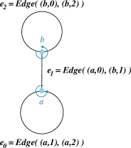
Figure 3: Representation of fatgraph edges. Each edge is identified with a pair of endpoints, where an endpoint is a vertex together with an attachment index. In the figure, letters $a$ and $b$ denote the vertices; attachment indices are computed by assigning index $0$ to the edge closest to the orientation arrow’s tail.

3.2.1 Computation of the edge list

The edge list ”$\mathitbf{G}$.edges” can be computed from the list of vertices as follows.

The total number $m$ of edges is computed from the sum of vertex valences, and used to create a temporary array $P$ of $m$ lists (each one initially empty). We then incrementally turn $P$ into a list of edge endpoints (in the form $(\mathitbf{v},a)$ where $\mathitbf{v}$ is a vertex and $a$ the attachment index) by just walking the list of vertices: $P[k]$ is the list ”[ $(\mathitbf{v}_{k},0)$, $\ldots$, $(\mathitbf{v}_{k},z_{k})$ ]” where $\mathitbf{v}_{k}$ (of valence $z_{k}$) is the $k$-th ”Vertex” in ”$\mathitbf{G}$.vertices”. The list ”$\mathitbf{G}$.edges” is just $P$ recast into ”Edge” objects. In pseudo-code:

⬇

1 $m$ $\leftarrow$ $(1/2)\cdot\sum_{\mathitbf{v}\in\mathitbf{G}.vertices}\text{valence}(\mathitbf{v})$

2 $P$ $\leftarrow$ array of $m$ empty lists

3 for $\mathitbf{v}$ in $\mathitbf{G}$.vertices:

4 for ($a$, $e$) in enumerate($\mathitbf{v}$):

5 append $(\mathitbf{v},a)$ to $P[e]$

6 wrap endpoints into ”Edge” objects

7 $\mathitbf{G}$.edges $\leftarrow$ [ Edge($p$) for $p$ in $P$ ]

3.3 Boundary Cycles

Definition 3.6.

A ”BoundaryCycle” object is a set of corners (see Figure 4).

A corner object $\mathitbf{C}$ is a triple ”(vertex, incoming, outgoing)”, consisting of a vertex $\mathitbf{v}$ and two indices ”$i$ == $\mathitbf{C}$.incoming”, ”$j$ == $\mathitbf{C}$.outgoing” of consecutive edges (in the cyclic order at $\mathitbf{v}$). In order to have a unique representation of any corner, we impose the condition that either $j=i+1$, or $i$ and $j$ are, respectively, the ending and starting indices of $\mathitbf{v}$ (regarded as a list).

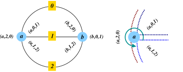
Figure 4: Representation of fatgraph boundary cycles. Left: How the boundary cycles are represented with corners: each boundary component is identified with the set of triplets it encloses. Therefore the boundary cycles for the graph are represented by the sets $\{(a,0,1),(b,2,0)\}$, $\{(a,1,2),(b,1,2)\}$, and $\{(a,2,0),(b,0,1)\}$. Right: Zoom around vertex $a$ in the left picture, to show the three corners identified with triples $(a,i,j)$. The indices in the triple are attachment indices, i.e., displacement relative from the ciliated edge (the one closest to the arrow tail); they bear no relation to the labels on the edges (numbers on the light yellow background in the left picture).

It is easy to convince oneself that a ”BoundaryCycle” object corresponds to a boundary cycle as defined in Section 3. Indeed, if $(L,\sigma_{0},\sigma_{1},\sigma_{2})$ is a fatgraph, then the boundary cycles are defined as the orbits of $\sigma_{2}$ on the set $L$ of half-edges; a (endpoint vertex, attachment index) pair uniquely identifies an half-edge and can thus be substituted for it. For computational efficiency reasons, we add an additional successor index to form the corner triple $(\mathitbf{v},i,j)$ so that the action of $\sigma_{2}$ can be computed from corner data alone, without any reference to the ambient fatgraph.

Since distinct orbits are disjoint, two ”BoundaryCycle” objects are either identical (they comprise the same corners) or have no intersection. In particular, this representation based on corners distinguishes boundary cycles made of the same edges: for instance, the boundary cycles of the fatgraph depicted in Figure 5 are represented by the disjoint set of corners $\{(\mathitbf{v},2,3),(\mathitbf{v},4,5),(\mathitbf{v},0,1)\}$ and $\{(\mathitbf{v},1,2),(\mathitbf{v},3,4),(\mathitbf{v},5,0)\}$.

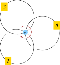
Figure 5: A fatgraph whose two boundary cycles are comprised of exactly the same edges; however, they give rise to disjoint sets of corners: $\{(\mathitbf{v},2,3),(\mathitbf{v},4,5),(\mathitbf{v},0,1)\}$ versus $\{(\mathitbf{v},1,2),(\mathitbf{v},3,4),(\mathitbf{v},5,0)\}$.

3.3.1 Computation of boundary cycles

The procedure for computing the set of boundary cycles of a given ”Fatgraph” object $\mathitbf{G}$ is listed in Algorithm 1.

Algorithm 1 Output the set of boundary cycles of a Fatgraph object $\mathitbf{G}$. Input to the algorithm is a Fatgraph object $\mathitbf{G}$; the output is a list of BoundaryCycle objects. The special constant used marks locations in the temporary array corners whose contents has already been assigned to a boundary cycle.

⬇

1 def compute_boundary_cycles($\mathitbf{G}$):

2 build working array of corners

3 corners $\leftarrow$ [ [ ($\mathitbf{v}$, $i$, ($(i+1)$ % $\lvert\mathitbf{v}\rvert$)) for $i$ in $0,\ldots,\lvert\mathitbf{v}\rvert-1$ ]

4 for $\mathitbf{v}$ in $\mathitbf{G}$.vertices ]

5 result $\leftarrow$ empty list

6 $l_{0}$ $\leftarrow$ 0

7 $i_{0}$ $\leftarrow$ 0

8 while True:

9 locate the first unused corner

10 for $l$ in $l_{0}$, $\ldots$, size(corners)-1:

11 $\mathitbf{v}$ $\leftarrow$ $\mathitbf{G}$.vertices[$l$]

12 $i$ $\leftarrow$ first_index_not_used(corners[$\mathitbf{v}$], $i_{0}$)

13 if $i$ is not None:

14 exit “for” loop

15 if $l$ $=$ size(corners)-1 and $i$ is None:

16 all corners used, mission accomplished

17 return result

18 else:

19 $l_{0}$ $\leftarrow$ $l$

20 $i_{0}$ $\leftarrow$ $i$

21 walk the boundary cycle and record corners

22 start $\leftarrow$ $(\mathitbf{v},i)$

23 triples $\leftarrow$ empty list

24 while $(\mathitbf{v},i)$ $\neq$ start or size(triples) $=$ 0:

25 triples.append(corners[$\mathitbf{v}$][$i$])

26 $j$ $\leftarrow$ corners[$v$][$i$][2]

27 $\mathitbf{e}$ $\leftarrow$ $\mathitbf{v}$[$j$]

28 mark location as “used”

29 corners[$\mathitbf{v}$][$i$] $\leftarrow$ used

30 $(\mathitbf{v},i)$ $\leftarrow$ other_end($\mathitbf{e}$, $\mathitbf{v}$, $j$)

31 $\mathitbf{b}$ $\leftarrow$ BoundaryCycle(triples)

32 result.append($\mathitbf{b}$)

33

34 def first_index_not_used($L$):

35 for index, item in enumerate($L$):

36 if item is not used:

37 return index

38 return None

The algorithm closely follows a geometrical procedure: starting with any corner, follow its “outgoing” edge to its other endpoint, and repeat until we come back to the starting corner. The list of corners so gathered is a boundary cycle. At each iteration, the used corners are cleared out of the ”corners” list by replacing them with the special value used, so that they will not be picked up again in subsequent iterations.

Lemma 3.1.

For any ”Fatgraph” object $\mathitbf{G}$ representing a fatgraph $G$, the function ”compute_boundary_cycles” in Algorithm 1 has the following properties: 1) terminates in finite time, and 2) returns a list of ”BoundaryCycle” objects that represent the boundary cycles of $G$.

Proof.

The algorithm works on a temporary array ”corners”: as it walks along a boundary cycle (lines 24–30), corner triples are moved from the working array to the ”triples” list and replaced with the constant used; when we’re back to the starting corner, a ”BoundaryCycle” object $\mathitbf{b}$ is constructed from the ”triples” list and appended to the result.

The ”corners” variable is a list, the $n$-th item of which is (again) a list holding the corners around the $n$-th vertex (i.e., ”$\mathitbf{G}$.vertices[$n$]”), in the order they are encountered when winding around the vertex. By construction, ”corners[$\mathitbf{v}$][$i$]” has the the form $(\mathitbf{v},i,j)$ where $j$ is the index following $i$ in the cyclic order, i.e., $(\mathitbf{v},i,j)$ represents the corner formed by the “incoming” $i$-th edge and the “outgoing” $j$-th edge.

The starting corner for each walk along a boundary cycle is determined by scanning the ”corners” list (lines 10–14): loop over all indexes $\mathitbf{v}$, $i$ in the ”corners” list, and quit looping as soon as ”corners[$\mathitbf{v}$][$i$]” is not used (line 13). If all locations in the corners list are used, then the all corners have been assigned to a boundary cycle and we can return the result list to the caller. ∎

3.4 Orientation

According to Definition 2.8, orientation is given by a total order of the edges (which directly translates into an orientation of the associated orbifold cell).

Definition 3.7.

The orientation ”$\mathitbf{G}$.orient” is a list that associates each edge with its position according to the order given by the orientation. Two such lists are equivalent if they differ by an even permutation.

If $\mathitbf{e}_{1}$ and $\mathitbf{e}_{2}$ are edges in a ”Fatgraph” object $\mathitbf{G}$, then $\mathitbf{e}_{1}$ precedes $\mathitbf{e}_{2}$ iff ”$\mathitbf{G}$.orient[$\mathitbf{e}_{1}$] ¡ $\mathitbf{G}$.orient[$\mathitbf{e}_{2}$]”; this links the fatgraph orientation from Definition 2.8 with the one above.

If a ”Fatgraph” object is derived from another ”Fatgraph” instance (e.g., when an edge is contracted), the resulting graph must derive its orientation from the “parent” graph, if we want the edge contraction to correspond to taking cell boundary in the orbicomplex $\mathcal{M}^{\text{comb}}_{g,n}$.

When no orientation is given, the trivial one is (arbitrarily) chosen: edges are ordered in the way they are listed in the ”$\mathitbf{G}$.edges” list, i.e., ”$\mathitbf{G}$.orient[$\mathitbf{e}$]” is the position at which $\mathitbf{e}$ appears in ”$\mathitbf{G}$.edges”.

According to Definition 2.9, a fatgraph is orientable iff it has no orientation-reversing automorphism. The author knows of no practical way to ascertain if a fatgraph is orientable other than enumerating all automorphisms and checking if any one of them reverses orientation:

⬇

1 def is_oriented($\mathitbf{G}$):

2 for $\mathitbf{a}$ in automorphisms($\mathitbf{G}$):

3 if is_orientation_reversing($\mathitbf{a}$):

4 return False

5 no orientation-reversing automorphism found, $\mathitbf{G}$ is orientable

6 return True

3.5 A category of Fatgraph objects

3.5.1 Isomorphisms of Fatgraph objects

In this section, we shall only give the definition of ”Fatgraph” isomorphisms and prove the basic properties; the algorithmic generation and treatment of ”Fatgraph” isomorphisms is postponed to Section 4.

Definition 3.8.

An isomorphism of ”Fatgraph” objects $\mathitbf{G}_{1}$ and $\mathitbf{G}_{2}$ is a triple $\mathitbf{f}=$”(pv, rot, pe)” where:

• ”pv” is a permutation of the vertices: vertex $\mathitbf{v}_{1}$ of $\mathitbf{G}_{1}$ is sent to vertex ”pv[$\mathitbf{v}$]” of $\mathitbf{G}_{2}$, and rotated by ”rot[$\mathitbf{v}$]” places leftwards;

• ”pe” is a permutation of the edge labels: edge $\mathitbf{e}$ in $\mathitbf{G}_{1}$ is mapped to edge ”pe[$\mathitbf{e}$]” in $\mathitbf{G}_{2}$.

The adjacency relation must be preserved by isomorphism triples: if $\mathitbf{v}_{1}$ and $\mathitbf{v}_{2}$ are endpoint vertices of the edge $\mathitbf{e}$, then ”pv[$\mathitbf{v}_{1}$]” and ”pv[$\mathitbf{v}_{2}$]” must be the endpoint vertices of edge ”pe[$\mathitbf{e}$]” in $\mathitbf{G}_{2}$.

Since a vertex in a ”Fatgraph” instance is essentially the list of labels of edges attached to that vertex, we can dually state the compatibility condition above as requiring that, for any vertex $\mathitbf{v}$ in ”$\mathitbf{G}_{1}$.vertices” and any valid index $j$ of an edge of $\mathitbf{v}$, we have:

$$\mathitbf{G}_{2} \mathitbf{v} j \mathitbf{v} = \mathitbf{G}_{1} \mathitbf{v} j$$.vertices[pv[]][+rot[]] pe[.vertices[][]] (5)

The above formula (5) makes the parallel between ”Fatgraph” object isomorphisms and fatgraph maps (in the sense of Definition 2.1) explicit.

Lemma 3.2.

Let $G_{1}$, $G_{2}$ be fatgraphs, represented respectively by $\mathitbf{G}_{1}$ and $\mathitbf{G}_{2}$. Every isomorphism of fatgraphs $f\colon G_{1}\to G_{2}$ lifts to a corresponding isomorphism ”$\mathitbf{f}$ == (pv, rot, pe)” on the computer representations. Conversely, every triple ”(pv, rot, pe)” representing an isomorphism between the ”Fatgraph” instances induces a (possibly trivial) fatgraph isomorphism between $G_{1}$ and $G_{2}$.

Proof.

Every isomorphism $f\colon G_{1}\to G_{2}$ naturally induces bijective maps $f_{V}\colon V(G_{1})\to V(G_{2})$ and $f_{E}\colon E(G_{1})\to E(G_{2})$ on vertices and edges. Given a cilium on every vertex, $f$ additionally determines, for each vertex $v\in V(G)$, the displacement $f_{\textsl{rot}}(v)$ of the image of the cilium of $v$ relative to the cilium of $f_{V}(v)$. Similarly, $f_{E}$ determines a bijective mapping of edge labels, and is completely determined by it. This is exactly the data collected in the triple ”(pv, rots, pe)”, and the compatibility condition (5) holds by construction.

Conversely, assume we are given a triple ”(pv, rots, pe)”, representing an isomorphism of ”Fatgraph” instances. We can construct maps $f_{V}$, $f_{E}$ as follows: $f_{V}$ sends a vertex $\mathitbf{v}\in\mathitbf{G}_{1}$ to the vertex corresponding to ”pv[$\mathitbf{v}$]”; $f_{E}$ maps the cilium of $\mathitbf{v}$ to the edge attached to ”pv[$\mathitbf{v}$]” at ”rot[$\mathitbf{v}$]” positions away from the cilium; the compatibility condition (5) guarantees that $f_{E}$ is globally well-defined. ∎

Lemma 3.3.

Let $\mathitbf{G}_{1}$, $\mathitbf{G}_{2}$ be ”Fatgraph” objects, and $\eta$ a bijective map between ”$\mathitbf{G}_{1}$.edges” and ”$\mathitbf{G}_{2}$.edges” that preserves the incidence relation. Then there is a unique ”Fatgraph” isomorphism $\mathitbf{f}$ that extends $\eta$ (in the sense that ”$\mathitbf{f}$.pe == $\eta$”).

Proof.

Start constructing the ”Fatgraph” morphism $\mathitbf{f}$ by setting ”$\mathitbf{f}$.pe == $\eta$”. If $\mathitbf{e}_{1}$, …, $\mathitbf{e}_{z_{k}}$ are the edges incident to ”$\mathitbf{v}_{k}\in\mathitbf{G}_{1}$.vertices”, then there is generally one and only one endpoint $\mathitbf{v}_{k}^{\prime}$ common to edges $\eta(\mathitbf{e}_{k})$; define ”$\mathitbf{f}$.pv[$\mathitbf{v}_{k}$] == $\mathitbf{v}_{k}^{\prime}$”. There is only one case in which this is not true, namely, if all edges share the same two endpoints: in this case, however, there is still only one choice of ”$\mathitbf{f}$.pv[$\mathitbf{v}_{k}$]” such that the cyclic order of edges at the source vertex matches the cyclic order of edges at the target vertex. Finally, choose ”$\mathitbf{f}$.rot[$\mathitbf{v}_{k}$]” as the displacement between the cilium at $\mathitbf{v}_{k}^{\prime}$ and the image of the cilium of $\mathitbf{v}_{k}$.

It is easy to check that eq. (5) holds, so $\mathitbf{f}$ is a well-defined isomorphism. ∎

3.5.2 Contraction morphisms

Recall from the definition in Section 2 that contraction produces a “child” fatgraph from a “parent” fatgraph and a chosen regular (i.e., non-looping) edge.

The ”Fatgraph.contract” method (see Algorithm 2) thus needs only take as input the “parent” graph $\mathitbf{G}$ and the edge $\mathitbf{e}$ to contract, and produces as output the “child” fatgraph $\mathitbf{G}^{\prime}$. The contraction algorithm proceeds in the following way:

• The two end vertices of the edge $\mathitbf{e}$ are fused into one: the list ”$\mathitbf{G}^{\prime}$.vertices” is built by copying the list ”$\mathitbf{G}$.vertices”, removing the two endpoints of $\mathitbf{e}$, and adding the new vertex (resulting from the collapse of $\mathitbf{e}$) at the end.

• Deletion of an edge also affects the orientation: the orientation ”$\mathitbf{G}^{\prime}$.orient” on the “child” fatgraph keeps the edges in the same order as they are in the parent fatgraph. However, since ”$\mathitbf{G}^{\prime}$.orient” must be a permutation of the edge indices, we need to renumber the edges and shift the higher-numbered edges down one place.

• The “child” graph $\mathitbf{G}^{\prime}$ is constructed from the list ”$\mathitbf{G}^{\prime}$.vertices” and the derived orientation ”$\mathitbf{G}^{\prime}$.orient”; the list of “new” edges is constructed according to the procedure given in Section 3.2.1.

Listing 2 summarizes the algorithm applied.

Algorithm 2 Construct a new Fatgraph object $\mathitbf{G}^{\prime}$ obtained by contracting the edge $\mathitbf{e}$ in $\mathitbf{G}$. The renumbering function $s$ is the identity on numbers in the range $0$, …, $e-1$, and shifts numbers in range $e+1$, …, $m$ down by 1. Function rotated$(L,p)$ returns a copy of list $L$ shifted leftwards by $p$ places.

⬇

1 def contract($\mathitbf{G}$, $\mathitbf{e}$):

2 let ($\mathitbf{v}_{1}$, $a_{1}$), ($\mathitbf{v}_{2}$, $a_{2}$) be the endpoints of $\mathitbf{e}$

3 $V^{\prime}$ $\leftarrow$ [ Vertex($x$ for $x$ in $\mathitbf{v}$ if $x$ $\neq$ $\mathitbf{e}$)

4 for $\mathitbf{v}$ in $\mathitbf{G}$.vertices if $\mathitbf{v}$ $\neq$ $\mathitbf{v}_{1}$ and $\mathitbf{v}$ $\neq$ $\mathitbf{v}_{2}$ ]

5 append the fused vertex at end of list $V$

6 $\mathitbf{v}^{\prime}$ $\leftarrow$ Vertex(rotated($\mathitbf{v}_{1}$, $a_{1}$) + rotated($\mathitbf{v}_{2}$, $a_{2}$))

7 $V^{\prime}$.append($\mathitbf{v}^{\prime}$)

8 $\omega^{\prime}$ $\leftarrow$ [ $s$($\mathitbf{G}^{\prime}$.orient[$x$]) for $x$ in $\mathitbf{G}^{\prime}$.edges if $x$ $\neq$ $e$ ]

9 return Fatgraph(vertices $\leftarrow$ $V^{\prime}$; orient $\leftarrow$ $\omega^{\prime}$)

The vertex resulting from the contraction of $\mathitbf{e}$ is formed as follows. Assume $\mathitbf{v}_{1}$ and $\mathitbf{v}_{2}$ are the endpoint vertices of the contracted edge. Now fuse endpoints of the contracted edge:

1. Rotate the lists $\mathitbf{v}_{1}$, $\mathitbf{v}_{2}$ so that the given edge $\mathitbf{e}$ appears last in $\mathitbf{v}_{1}$ and first in $\mathitbf{v}_{2}$.

2. Form the new vertex $\mathitbf{v}$ by concatenating the two rotated lists (after expunging vertices $\mathitbf{v}_{1}$ and $\mathitbf{v}_{2}$).

Note that this changes the attachment indices of all edges incident to $\mathitbf{v}_{1}$ and $\mathitbf{v}_{2}$, therefore the edge list of $\mathitbf{G}^{\prime}$ needs to be recomputed from the vertex list.

The “child” fatgraph $G^{\prime}$ inherits an orientation from the “parent” fatgraph, which might differ from its default orientation. Let $\alpha_{1},\ldots,\alpha_{h},\ldots,\alpha_{m}$ be the edges of the parent fatgraph $G$, with $e=\alpha_{h}$ being contracted to create the “child” graph $G^{\prime}$. If $\alpha_{k(1)}<\alpha_{k(2)}<\ldots<\alpha_{k(m)}$ is the ordering on $E(G)$ that induces the orientation on $G$ and $h=k(j)$, then $\alpha_{k(1)}<\ldots<\alpha_{k(j-1)}<\alpha_{k(j+1)}<\ldots<\alpha_{k(m)}$ descends to a total order on the edges of $G^{\prime}$ and induces the correct orientation.

Orientation is represented in a ”Fatgraph” object as a list, mapping edge labels to a position in the total order; using the notation above, the orientation of $G$ is given by $\omega:=k^{-1}$. The orientation on $G^{\prime}$ is then given by $\omega^{\prime}$ defined as follows:

$$\omega^{\prime}(i):=\begin{cases}\omega(i)&\text{if $\omega(i)<h$,}\\ \omega(i)-1&\text{if $\omega(i)>h$.}\end{cases}$$

Alternatively we can write:

$$\omega^{\prime}=s\circ\omega,\qquad s(x):=\begin{cases}x&\text{if $x<h$,}\\ x-1&\text{if $x>h$.}\end{cases}$$

This corresponds exactly to the assignment in Algorithm 2.

The above discussion can be summarized in the following.

Lemma 3.4.

If $\mathitbf{G}$ and $\mathitbf{G}^{\prime}$ represent fatgraphs $G$ and $G^{\prime}$, and ”$\mathitbf{G}$ == contract($\mathitbf{G}^{\prime}$, $\mathitbf{e}$)”, then $G$ is obtained from $G^{\prime}$ by contraction of the edge $e$ represented by $\mathitbf{e}$.

The contract_boundary_cycle function.

The boundary cycles of the “child” ”Fatgraph” object $\mathitbf{G}^{\prime}$ can also be computed from those of $\mathitbf{G}$. The implementation (see Listing 1) is quite straightforward: we copy the given list of corners and alter those who refer to the two vertices that have been merged in the process of contracting the specified edge.

Algorithm 3 Return a new BoundaryCycle instance, image of $\mathitbf{b}$ under the topological map that contracts the edge with index $\mathitbf{e}$.

⬇

1 def contract_boundary_cycle($\mathitbf{G}$, $\mathitbf{b}$, $\mathitbf{e}$):

2 let ($\mathitbf{v}_{1}$, $a_{1}$), ($\mathitbf{v}_{2}$, $a_{2}$) be the endpoints of $\mathitbf{e}$

3 $z_{1}$ $\leftarrow$ valence($\mathitbf{v}_{1}$)

4 $z_{2}$ $\leftarrow$ valence($\mathitbf{v}_{2}$)

5 “child” boundary cycle $\mathitbf{b}^{\prime}$ starts off as an empty list

6 $\mathitbf{b}^{\prime}$ $\leftarrow$ [ ]

7 for corner in $\mathitbf{b}$:

8 if corner[0] $=$ $\mathitbf{v}_{1}$:

9 if $a_{1}$ $=$ corner.incoming:

10 continue with next corner

11 else:

12 $i_{1}$ $\leftarrow$ (corner.incoming - $a_{1}$ - 1) % $z_{1}$

13 $i_{2}$ $\leftarrow$ (corner.outgoing - $a_{1}$ - 1) % $z_{1}$

14 append corner ($\mathitbf{v}_{1}$, $i_{1}$, $i_{2}$) to $\mathitbf{b}^{\prime}$

15 elif corner[0] $=$ $\mathitbf{v}_{2}$:

16 if $a_{2}$ $=$ corner.incoming:

17 continue with next corner

18 if $a_{2}$ $=$ corner.outgoing:

19 append $(\mathitbf{v}_{1},z_{1}+z_{2}-3,0)$ to $\mathitbf{b}^{\prime}$

20 else:

21 $i_{1}$ $\leftarrow$ $z_{1}-1$ + ((corner.incoming - $a_{2}$ - 1) % $z_{2}$)

22 $i_{2}$ $\leftarrow$ $z_{1}-1$ + ((corner.outgoing - $a_{2}$ - 1) % $z_{2}$)

23 append $(v_{1},i_{1},i_{2})$ to $b^{\prime}$

24 else:

25 keep corner unchanged

26 append corner to $\mathitbf{b}^{\prime}$

27 return BoundaryCycle($\mathitbf{b}^{\prime}$)

Let $\mathitbf{v}_{1}$ and $\mathitbf{v}_{2}$ be the end vertices of the edge to be contracted, and $a_{1}$, $a_{2}$ be the corresponding attachment indices. Let $z_{1}$ and $z_{2}$ be the valences of vertices $\mathitbf{v}_{1}$, $\mathitbf{v}_{2}$. We build the list of corners of the boundary cycle in the “child” graph incrementally: the $\mathitbf{b}^{\prime}$ lists starts empty (line 6), and is then added corners as we run over them in the loop between lines 7 and 26.

There are four distinct corners that are bounded by the edge $\mathitbf{e}$ to be contracted; denote them by $\mathitbf{C}_{1}$, $\mathitbf{C}_{2}$, $\mathitbf{C}_{3}$, $\mathitbf{C}_{4}$. These map onto two distinct corners $\mathitbf{C}$, $\mathitbf{C}^{\prime}$ after contraction. Assume that $\mathitbf{C}_{1}$ and $\mathitbf{C}_{2}$ map to $\mathitbf{C}$: then $\mathitbf{C}_{1}$ and $\mathitbf{C}_{2}$ lie “on the same side” of the contracted edge, i.e., any boundary cycle that includes $\mathitbf{C}_{1}$ will include also $\mathitbf{C}_{2}$ and viceversa. (See Figure 6 for an illustration.) Since they both map to the same corner $\mathitbf{C}$ in the “child” graph, we only need to keep one: we choose to keep (and transform) the corner that has the contracted edge at the second index (lines 9–10); similarly for $\mathitbf{C}_{3}$ and $\mathitbf{C}_{4}$ in mapping to $\mathitbf{C}^{\prime}$ (lines 16–17).

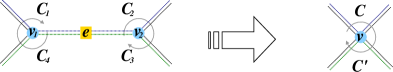
Figure 6: How corners are modified by edge contraction. Left: Four distinct corners are formed at the endpoints $\mathitbf{v}_{1}$, $\mathitbf{v}_{2}$ of edge $\mathitbf{e}$, which is to be contracted: $\mathitbf{C}_{1}=(\mathitbf{v}_{1},0,2)$, $\mathitbf{C}_{2}=(\mathitbf{v}_{2},0,1)$, $\mathitbf{C}_{3}=(\mathitbf{v}_{2},1,2)$, and $\mathitbf{C}_{4}=(\mathitbf{v}_{1},0,1)$. Edges are shown thickened, and (potentially) distinct boundary cycles are drawn in different colors. Right: After contraction of $\mathitbf{e}$, corners $\mathitbf{C}_{1}$ and $\mathitbf{C}_{2}$ are fused into $C=(\mathitbf{v},0,1)$, and $\mathitbf{C}_{3}$, $\mathitbf{C}_{4}$ are fused into $\mathitbf{C}^{\prime}=(\mathitbf{v},2,3)$.

Recall that, when contracting an edge with endpoints $\mathitbf{v}_{1}$ and $\mathitbf{v}_{2}$, the new vertex is formed by concatenating two series of edges: (1) edges attached to the former $\mathitbf{v}_{1}$, starting with the successor (in the cyclic order) of the contracted edge; (2) edges attached to the former $\mathitbf{v}_{2}$, starting with the successor of the contracted edge. Therefore:

1. The image of a corner rooted in vertex $\mathitbf{v}_{1}$ will have its attachment indices rotated leftwards by $a_{1}+1$ positions: the successor of the contracted edge has now attachment index 0 (lines 12–13). Note that the highest attachment index belonging into this group is $z_{1}-2$: position $z_{1}-1$ would correspond to the contracted edge.

2. The image of a corner rooted in vertex $\mathitbf{v}_{2}$ has its attachment indices rotated leftwards by $a_{2}+1$ positions, and shifted up by $z_{1}-1$ (lines 21–22). As a special case, when the contracted edge is in second position we need to map the corner to the corner having attachment index 0 in second position (line 19).

Any other corner is copied with no alterations (line 26).

3.5.3 The category of Fatgraph objects

We can now formally define a category of ”Fatgraph” objects and their morphisms.

Definition 3.9.

$\mathcal{R}^{\#}$ is the category whose objects are ”Fatgraph” objects, and whose morphisms are compositions of ”Fatgraph” isomorphisms (as defined in Section 4) and edge contraction maps.

More precisely, if $\mathitbf{G}$ and $\mathitbf{G}^{\prime}$ are isomorphic ”Fatgraph” objects, then the morphism set $\mathcal{R}^{\#}(\mathitbf{G},\mathitbf{G}^{\prime})$ is defined as the set of ”Fatgraph” isomorphisms in the sense of Section 4; otherwise, let $m$ and $m^{\prime}$ be the number of edges of $\mathitbf{G}$, $\mathitbf{G}^{\prime}$, and set $k:=m-m^{\prime}$: each element in $\mathcal{R}^{\#}(\mathitbf{G},\mathitbf{G}^{\prime})$ has the form $\mathitbf{a}^{\prime}\circ(\pi_{1}\circ\cdots\circ\pi_{k})\circ\mathitbf{a}$ where $\mathitbf{a}$, $\mathitbf{a}^{\prime}$ are automorphisms of $\mathitbf{G}$, $\mathitbf{G}^{\prime}$ and $\pi_{1}$, …, $\pi_{k}$ are non-loop edge contractions.

Theorem 3.1.

There exists a functor $K$ from the category $\mathcal{R}^{\#}$ of ”Fatgraph” objects to the category $\mathcal{R}$ of abstract fatgraphs, which is surjective and full.

Proof.

Given a ”Fatgraph” $\mathitbf{G}$, its constituent ”Vertex” objects determine cyclic sequences $v_{0}=(e_{0}^{0},e^{0}_{1},\ldots,e^{0}_{z_{0}})$, …, $v_{l}=(e^{l}_{0},\ldots,e^{l}_{z_{l}})$, such that

$$\{e^{0}_{0},\ldots,e^{0}_{z_{0}},e^{1}_{0},\ldots,e^{l-1}_{z_{l-1}},e^{l}_{0},\ldots,e^{l}_{z_{l}}\}=\{0,\ldots,m-1\}.$$

Fix a starting element for each of the cyclic sequences $v_{0}$, …, $v_{l}$. Then set:

$$L:=\{(e,i,v):v=v_{j}\in\{v_{0},\ldots,v_{l}\},\;e=e^{j}_{i}\in v\},$$

and define maps $\sigma_{0},\sigma_{1},\sigma_{2}\colon L\to L$ as follows:

• $\sigma_{0}$ sends $(e,i,v_{j})$ to $(e^{\prime},i^{\prime},v_{j})$ where $i^{\prime}=(i+1)\%z_{j}$ and $e^{\prime}=e^{j}_{i^{\prime}}$ is the successor of $e$ in the cyclic order at $v_{j}$;

• $\sigma_{1}$ maps $(e,i,v)$ to the unique other triplet $(e^{\prime},i^{\prime},v^{\prime})\in L$ such that $e=e^{\prime}$;

• finally, $\sigma_{2}$ is determined by the constraint $\sigma_{0}\circ\sigma_{2}=\sigma_{1}$.

Then $K(\mathitbf{G})=(L,\sigma_{0},\sigma_{1},\sigma_{2})$ is a fatgraph. Figure 7 provides a graphical illustration of the way a ”Fatgraph” object is constructed out of such combinatorial data.

Now let $G$ be an abstract fatgraph; assuming $G$ has $m$ edges, assign to each edge a “label”, i.e., pick a bijective map $e:E(G)\to E$, where $E$ is an arbitrary finite set. Each vertex $v\in V(G)$ is thus decorated with a cyclic sequence of edge labels; the set of which determines a ”Fatgraph” object $\mathitbf{G}$; it is clear that $G=K(\mathitbf{G})$.

This proves that $K$ is surjective; since every fatgraph morphism can be written as a composition of isomorphisms and edge contractions (Lemma 2.1), it is also full. It is clear that every edge contraction is the image of an edge contraction in the corresponding ”Fatgraph” objects, and the assertion for isomorphisms follows as a corollary of Lemma 3.2. ∎

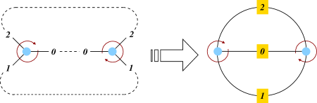
Figure 7: Construction of a fatgraph out of a set of Vertex instances: half-edges tagged with the same (numeric) label are joined together to form an edge.

Definition 3.10.

If $G=K(\mathitbf{G})$ then we say that the ”Fatgraph” object $\mathitbf{G}$ represents the abstract fatgraph $G$.

It is clear from the construction above that there is a considerable amount of arbitrary choices to be made in constructing a representative ”Fatgraph”; there are thus many representatives for the same fatgraph, and different choices lead to equivalent ”Fatgraph” objects.

Lemma 3.5.

Two distinct ”Fatgraph” objects representing the same abstract fatgraph are isomorphic.

Proof.

Assume $\mathitbf{G}_{1}$ and $\mathitbf{G}_{2}$ both represent the same abstract fatgraph $G=K(\mathitbf{G}_{1})=K(\mathitbf{G}_{2})$. Let $\eta_{1}$, $\eta_{2}$ be the maps that send ”Edge” objects in $\mathitbf{G}_{1}$, $\mathitbf{G}_{2}$ to the corresponding edges in $G$; then $\eta=\eta_{1}^{-1}\circ\eta_{2}$ maps edges of $\mathitbf{G}_{1}$ into edges of $\mathitbf{G}_{2}$ and respects the incidence relation, therefore it is the edge part of a ”Fatgraph” isomorphism by Lemma 3.3. ∎

Theorem 3.2.

The categories $\mathcal{R}^{\#}$ and $\mathcal{R}$ are equivalent.

Proof.

The functor $K$ is surjective and full by Theorem 3.1; that it is also faithful follows from the following argument. Any fatgraph morphism is a composition of edge contractions and isomorphisms. Any isomorphism determines, in particular, a map on the set of edges, and there is one and only one ”Fatgraph” isomorphism induced by this map (Lemma 3.3). Any edge contraction is uniquely determined by the contracted edge: if $f\colon G_{1}\to G_{2}$ is the morphism contracting edge $e$ and $G_{i}=K(\mathitbf{G}_{i})$, then $\mathitbf{f}$, contraction of the ”Edge” object $\mathitbf{e}$ representing $e$, is the sole morphism of $\mathitbf{G}_{1}$ into $\mathitbf{G}_{2}$ that maps onto $f$. ∎

4 Fatgraphs isomorphism and equality testing

The isomorphism problem on computer representations of fatgraphs consists in finding out when two distinct ”Fatgraph” instances represent isomorphic fatgraphs (in the sense of Definition 2.1) or possibly the same fatgraph. Indeed, the procedure for associating a ”Fatgraph” instance to an abstract fatgraph (see Theorem 3.1) involves labeling all edges, choosing a starting edge (cilium) on each vertex and enumerating all vertices in a certain order; for each choice, we get a different ”Fatgraph” instance representing the same (abstract) fatgraph.

The general isomorphism problem for (ordinary) graphs is a well-known difficult problem. However, the situation is much simpler for fatgraphs, because of the following property.

Lemma 4.1 (Rigidity Property).

Let $G_{1}$, $G_{2}$ be connected fatgraphs, and $f\colon G_{1}\to G_{2}$ an isomorphism. For any vertex $v\in V(G_{1})$, and any edge $x$ incident to $v$, $f$ is uniquely determined (up to homotopies fixing the vertices of $G_{i}$) by its restriction to $v$ and $x$.

In particular, an isomorphism of graphs with ciliated vertices is completely determined once the image $w=f(v)$ of a vertex $v$ is known, together with the displacement (relative to the cyclic order at $w$) of the image of the cilium of $v$ relative to the cilium of the image vertex $w$.

Proof.

Consider $f$ as a CW-complex morphism: $f=(f_{0},f_{1})$ where $f_{i}$ is a continuous map on the set of $i$-dimensional cells.

Let $U$ be a small open neighborhood of $v\in V(G_{1})$. Given $f|_{U}$, incrementally construct a CW-morphism $f^{\prime}\colon G_{1}\to G_{2}$ as follows. Each edge $x^{\prime}$ incident to $v$ can be expressed as $x^{\prime}=\sigma_{0}^{\alpha}x$ for some ”$0\leqslant\alpha<$valence($v$)”. Let $w=f(v)$ and $y=f(x)$, and define:

$$f_{1}^{\prime}(x) :=y,$$

$$f_{0}^{\prime}(v) :=w,$$

$$f_{1}^{\prime}(x^{\prime}) :=\sigma_{0}^{\alpha}y=\sigma_{0}^{\alpha}f_{1}^{\prime}(x)\quad\text{if $x^{\prime}=\sigma_{0}^{\alpha}x$},$$

$$f_{0}^{\prime}(v^{\prime}_{\alpha}) :=w^{\prime}_{\alpha},$$

where:

• $v^{\prime}_{\alpha}$ is the endpoint of $x^{\prime}=\sigma_{0}^{\alpha}x$ “opposite” to $v$,

• $w^{\prime}_{\alpha}$ is the endpoint of $y^{\prime}=\sigma_{0}^{\alpha}y$ “opposite” to $w$.

Then $f^{\prime}$ extends $f$ on an open set $U^{\prime}\supsetneq\overline{U}$, which contains the subgraph formed by all edges attached to $v$ and $v^{\prime}$. In addition:

• $f^{\prime}_{1}(x^{\prime})=f(x^{\prime})$ up to a homotopy fixing the endpoints since $f$ commutes with $\sigma_{0}$,

• $f^{\prime}_{0}(v_{\alpha})=f(v_{\alpha})$ since $f$ preserves adjacency.

By repeating the same construction about the vertices $v^{\prime}_{\alpha}$ and $w^{\prime}_{\alpha}$, one can extend $f^{\prime}$ to a CW-morphism that agrees with $f$ on an open set $U^{\prime\prime}\supsetneq\overline{U^{\prime}}$.

Recursively, by connectedness, we can thus extend $f^{\prime}$ to agree with $f$ (up to homotopy) over all of $G_{1}$. ∎

4.1 Enumeration of Fatgraph isomorphisms

The stage is now set for presenting the algorithm to enumerate the isomorphisms between two given ”Fatgraph” objects. Pseudo-code is listed in Algorithm 4; as this procedure is quite complex, a number of auxiliary functions have been used, whose purpose is explained in Section 4.1.1. Function isomorphisms, given two ”Fatgraph” objects $\mathitbf{G}_{1}$ and $\mathitbf{G}_{2}$, returns a list of triples ”(pv, rot, pe)”, each of which determines an isomorphism. If there is no isomorphism connecting the two graphs, then the empty list ”[ ]” is returned.

Algorithm 4 Enumerate isomorphisms between two Fatgraph objects $\mathitbf{G}_{1}$ and $\mathitbf{G}_{2}$: output of the algorithm is a list of triples (pv, rot, pe). If there is no isomorphism connecting the two input fatgraphs, the empty list is returned.

⬇

1def isomorphisms($\mathitbf{G}_{1}$, $\mathitbf{G}_{2}$):

2 immediately rule out easy cases of no isomorphisms

3 if graphs invariants differ:

4 return [ ]

5 result $\leftarrow$ [ ]

6 vs1 $\leftarrow$ valence_spectrum($\mathitbf{G}_{1}$)

7 vs2 $\leftarrow$ valence_spectrum($\mathitbf{G}_{2}$)

8 (valence, vertices) $\leftarrow$ starting_vertices($\mathitbf{G}_{2}$)

9 $\mathitbf{v}_{1}$ $\leftarrow$ vs1[valence][0]

10 for $\mathitbf{v}_{2}$ in compatible_vertices($\mathitbf{v}_{1}$, vertices):

11 for rot in $0,\ldots,$valence:

12 Initializepv, rots, peas empty maps

13 pv[$\mathitbf{v}_{1}$] $\leftarrow$ $\mathitbf{v}_{2}$

14 rots[$\mathitbf{v}_{1}$] $\leftarrow$ rot

15 extend_map(pe, $\mathitbf{v}_{1}$, rotated($\mathitbf{v}_{2}$, rot))

16 if extension failed:

17 continue with next rot

18 breadth-first search to extend the mapping over corresponding vertices

19 nexts $\leftarrow$ neighbors(pv, pe, $\mathitbf{G}_{1}$, $\mathitbf{v}_{1}$, $\mathitbf{G}_{2}$, $\mathitbf{v}_{2}$)

20 while size(pv) < $\mathitbf{G}_{1}$.num_vertices:

21 neighborhood $\leftarrow$ [ ]

22 for ($\mathitbf{v}_{1}^{\prime}$, $\mathitbf{v}_{2}^{\prime}$, $r$) in nexts:

23 (pv, rots, pe) $\leftarrow$ extend_iso(pv, rots, pe, $\mathitbf{G}_{1}$, $\mathitbf{v}_{1}^{\prime}$, $r$, $\mathitbf{G}_{2}$, $\mathitbf{v}_{2}^{\prime}$)

24 if cannot extend:

25 exit “while” loop and continue with next rot

26 append neighbors(pv, pe, $\mathitbf{G}_{1}$, $\mathitbf{v}_{1}^{\prime}$, $\mathitbf{G}_{2}$, $\mathitbf{v}_{2}^{\prime}$) to neighborhood

27 nexts $\leftarrow$ neighborhood

28 isomorphism found, record it

29 result.append((pv, rots, pe))

30 return result

By the rigidity lemma 4.1, any fatgraph isomorphism is uniquely determined by the mapping of a small neighborhood of any vertex. The overall strategy of the algorithm is thus to pick a pair of “compatible” vertices and try to extend the map as in the proof of of lemma 4.1.

We wish to stress the difference with isomorphism of ordinary graphs: since an isomorphism $f$ is uniquely determined by any pair of corresponding vertices, the initial choice of candidates $v$, $f(v)$ either yields an isomorphism or it does not: there is no backtracking involved.

Since the isomorphism computation is implemented as an exhaustive search, it is worth doing a few simple checks to rule out cases of non-isomorphic graphs (lines 3–4). One has to weigh the time taken to compute a graph invariant versus the potential speedup obtained by not running the full scan of the search space; experiments run using the Python code show that the following simple invariants already provide some good speedup:

• the number of vertices, edges, boundary cycles;

• the total number of loops;

• the set of valences;

• the number of vertices of every given valence.

Since an isomorphism is uniquely determined by its restriction to any vertex, one can restrict to considering just pairs of the form $(\mathitbf{v}_{1},\mathitbf{v}_{2})$ where $\mathitbf{v}_{1}$ is a chosen vertex in $\mathitbf{G}_{1}$. Then the algorithm tries all possible ways (rotations) of mapping $\mathitbf{v}_{1}$ into a compatible vertex $\mathitbf{v}_{2}$ in $\mathitbf{G}_{2}$. The body of the inner loop (line 11 onwards) mimics the construction in the proof of Lemma 4.1.

The starting vertex $\mathitbf{v}_{1}$ should be selected so to minimize the number of mapping attempts performed; this is currently done by minimizing the product of valence and number of vertices of that valence on $\mathitbf{G}_{2}$ (line 8), and then picking a vertex of the chosen valence in $\mathitbf{G}_{1}$ as $\mathitbf{v}_{1}$ (line 9).

First, given the target vertex $\mathitbf{v}_{2}$ and a rotation ”rot”, a new triple ”(pv,rots,pe)” is created; ”pv” is set to represent the initial mapping of $\mathitbf{v}_{1}$ onto $\mathitbf{v}_{2}$, rotated leftwards by ”rot” positions, and ”pe” maps edges of $\mathitbf{v}_{1}$ into corresponding edges of the rotated $\mathitbf{v}_{2}$. If this mapping is not possible (e.g., $\mathitbf{v}_{1}$ has a loop and $\mathitbf{v}_{2}$ does not, or not in a corresponding position), then the attempt is aborted and execution continues from line 11 with the next candidate ”rot”.

The mapping defined by ”(pv,rots,pe)” is then extended to neighbors of the vertices already inserted. This entails a breadth-first search over pairs of corresponding vertices, starting from $\mathitbf{v}_{1}$ and $\mathitbf{v}_{2}$. Note that, in this extension step, not only the source and target vertices, but also the rotation to be applied is uniquely determined: chosen a vertex $\mathitbf{v}_{1}^{\prime}$ connected to $\mathitbf{v}_{1}$ by an edge $\mathitbf{e}$, there is a unique rotation $r$ on $\mathitbf{v}_{2}^{\prime}$ such that ”pv[$\mathitbf{e}$]” has the same attachment index to $\mathitbf{v}_{2}^{\prime}$ that $\mathitbf{e}$ has to $\mathitbf{v}_{1}$. If, at any stage, the extension of the current triple ”(pv, rots, pe)” fails, it is discarded and execution continues from line 11 with the next value of ”rot”.

When the loop started at line 10 is over, execution reaches the end of the ”isomorphisms” function, and returns the (possibly empty) list of isomorphisms to the caller.

Theorem 4.1.

Given ”Fatgraph” objects $\mathitbf{G}_{1}$, $\mathitbf{G}_{2}$, function ”isomorphisms” returns all ”Fatgraph” isomorphisms from $\mathitbf{G}_{1}$ to $\mathitbf{G}_{2}$.

Proof.

Given an isomorphism $f:\mathitbf{G}_{1}\to\mathitbf{G}_{2}$, restrict $f$ to the starting vertex $\mathitbf{v}_{1}$: then $f$ will be output when Algorithm 4 examines the pair $\mathitbf{v}_{1}$, $f(\mathitbf{v}_{1})$; since Algorithm 4 performs an exhaustive search, $f$ will not be missed.

Conversely, since equation (5) holds by construction for all the mappings returned by ”isomorphisms”, then each returned triple $\mathitbf{f}=$”(pv, rots, pe)” is an isomorphism. ∎

4.1.1 Auxiliary functions

Here is a brief description of the auxiliary functions used in the listing of Algorithm 4 and 5. Apart from the neighbors function, they are all straightforward to implement, so only a short specification of the behavior is given, with no accompanying pseudo-code.

The neighbors function.

Definition 4.1.

Define a candidate extension as a triplet ”($\mathitbf{v}_{1}^{\prime}$, $\mathitbf{v}_{2}^{\prime}$, $r$)”, where:

• $\mathitbf{v}_{1}^{\prime}$ is a vertex in $\mathitbf{G}_{1}$, connected to $\mathitbf{v}_{1}$ by an edge $\mathitbf{e}$;

• $\mathitbf{v}_{2}^{\prime}$ is a vertex in $\mathitbf{G}_{2}$, connected to $\mathitbf{v}_{2}$ by edge ”$\mathitbf{e}^{\prime}$ == pe[$\mathitbf{e}$]”;

• $r$ is the rotation to be applied to $\mathitbf{v}_{2}^{\prime}$ so that edge $\mathitbf{e}$ and $\mathitbf{e}^{\prime}$ have the same attachment index, i.e., they are incident at corresponding positions in $\mathitbf{v}_{1}^{\prime}$ and $\mathitbf{v}_{2}^{\prime}$.

Function ”neighbors” lists candidate extensions that extend map ”pv” in the neighborhood of given input vertices $\mathitbf{v}_{1}$ (in the domain fatgraph $\mathitbf{G}_{1}$) and $\mathitbf{v}_{2}$ (in the image fatgraph $\mathitbf{G}_{2}$). It outputs a list of triplets $(\mathitbf{v}_{1}^{\prime},\mathitbf{v}_{2}^{\prime},r)$, each representing a candidate extension.

Algorithm 5 Enumerate the candidate extensions of the given pv and pe in the neighborhood of input vertices $\mathitbf{v}_{1}$ and $\mathitbf{v}_{2}$.

⬇

1 def neighbors(pv, pe, $\mathitbf{G}_{1}$, $\mathitbf{v}_{1}$, $\mathitbf{G}_{2}$, $\mathitbf{v}_{2}$):

2 result $\leftarrow$ [ ]

3 for each non-loop edge $\mathitbf{e}$ attached to $\mathitbf{v}_{1}$:

4 let $(\mathitbf{v}_{1}^{\prime},a_{1})$ be the endpoint of $\mathitbf{e}$ distinct from $\mathitbf{v}_{1}$

5 if $\mathitbf{v}_{1}^{\prime}$ already in pv domain:

6 continue with next $\mathitbf{e}$

7 let $(\mathitbf{v}_{2}^{\prime},a_{2})$ be the endpoint of $\mathitbf{e}^{\prime}$=pe[$\mathitbf{e}$] distinct from $\mathitbf{v}_{2}$

8 if $\mathitbf{v}_{2}^{\prime}$ already in pv image:

9 continue with next $\mathitbf{e}$

10 result.append($(\mathitbf{v}_{1}^{\prime},\mathitbf{v}_{2}^{\prime},a_{1}-a_{2})$)

11 return result

A sketch of this routine is given in Algorithm 5. Two points are worth of notice:

1. By the time neighbors is called (at lines 19 and 26 in Algorithm 4), the map ”pe” has already been extended over all edges incident to $\mathitbf{v}_{1}$, so we can safely set $\mathitbf{e}^{\prime}=$”pe[$\mathitbf{e}$]” in neighbors.

2. Algorithm 4 only uses neighbors with the purpose of extending ”pv” and ”pe”, so neighbors ignores vertices that are already in the domain or image of ”pv”.

The valence_spectrum function.

The auxiliary function valence_spectrum, given a ”Fatgraph” instance $\mathitbf{G}$, returns a mapping that associates to each valence $z$ the list $V_{z}$ of vertices of $\mathitbf{G}$ with valence $z$.

The starting_vertices function.

For each pair $(z,V_{z})$ in the valence spectrum, define its intensity as the product $z\cdot\lvert V_{z}\rvert$ (valence times the number of vertices with that valence). The function starting_vertices takes as input a ”Fatgraph” object $\mathitbf{G}$ and returns the pair $(z,V_{z})$ from the valence spectrum that minimizes intensity. In case of ties, the pair with the largest $z$ is chosen.

The compatible and compatible_vertices functions.

Function compatible takes a pair of vertices $\mathitbf{v}_{1}$ and $\mathitbf{v}_{2}$ as input, and returns boolean ”True” iff $\mathitbf{v}_{1}$ and $\mathitbf{v}_{2}$ have the same invariants. (This is used as a short-cut test to abandon a candidate mapping before trying a full adjacency list extension, which is computationally more expensive.) The sample code uses valence and number of loops as invariants.

The function compatible_vertices takes a vertex $\mathitbf{v}$ and a list of vertices $L$, and returns the list of vertices in $L$ that are compatible with $\mathitbf{v}$ (i.e., those which $\mathitbf{v}$ could be mapped to).

The extend_map and extend_iso functions.

The extend_map function takes as input a mapping ”pe” and a pair of ciliated vertices $\mathitbf{v}_{1}$ and $\mathitbf{v}_{2}$, and alters ”pe” to map edges of $\mathitbf{v}_{1}$ to corresponding edges of $\mathitbf{v}_{2}$: the cilium to the cilium, and so on: ”pe[$\sigma_{0}^{\alpha}(\mathitbf{e})$] == $\sigma_{0}^{\alpha}$(pe[$\mathitbf{e}$])”. If this extension is not possible, an error is signaled to the caller.

The extend_iso function is passed a ”(pv, rots, pe)” triplet, a vertex $\mathitbf{v}_{1}^{\prime}$ of $\mathitbf{G}_{1}$, a vertex $\mathitbf{v}_{2}^{\prime}$ of $\mathitbf{G}_{2}$ and a rotation $r$; it alters the given ”(pv,rots,pe)” triple by adding a mapping of the vertex $\mathitbf{v}_{1}^{\prime}$ into vertex $\mathitbf{v}_{2}^{\prime}$ (and rotating the target vertex by ”r” places rightwards). If the extension is successful, it returns the extended map ”(pv, rot, pe)”; otherwise, signals an error.

4.2 Operations with Fatgraph Isomorphisms

Compare pull-back orientation.

The compare_orientations function takes an isomorphism triple ”(pv, rots, pe)” and a pair of ”Fatgraph” objects $\mathitbf{G}_{1}$ , $\mathitbf{G}_{2}$, and returns $+1$ or $-1$ depending on whether the orientations of the target ”Fatgraph” pulls back to the orientation of the source ”Fatgraph” via the given isomorphism.

Recall that for a ”Fatgraph” object $\mathitbf{G}$, the orientation is represented by a mapping ”$\mathitbf{G}$.orient” that associates an edge $\mathitbf{e}$ with its position in the wedge product that represents the orientation; therefore, the pull-back orientation according to an isomorphism ”(pv, rots, pe)” from $\mathitbf{G}$ to $\mathitbf{G}^{\prime}$ is simply given by the map ”$\mathitbf{e}$ $\mapsto$ $\mathitbf{G}^{\prime}$.orient[pe[$\mathitbf{e}$]]”. Thus, the comparison is done by constructing the permutation that maps ”$\mathitbf{G}$.orient[$\mathitbf{e}$]” to ”$\mathitbf{G}^{\prime}$.orient[pe[$\mathitbf{e}$]]” and taking its sign (which has linear complexity with respect to the number of edges).

The is_orientation_reversing function.

Determining whether an automorphism reverses orientation is crucial for knowing which fatgraphs are orientable. Function is_orientation_reversing takes a ”Fatgraph” object and an isomorphism triple ”(pv, rots, pe)” as input, and returns boolean ”True” iff the isomorphism reverses orientation. This amounts to checking whether the given orientation and that of the pull-back one agree, which can be done with the comparison method discussed above.

Transforming boundary cycles under an isomorphism.

The function transform_boundary_cycle is used when comparing marked fatgraphs: as the marking is a function on the boundary cycles, we need to know exactly which boundary cycle of the target graph corresponds to a given boundary cycle in the source graph.

Recall that ”BoundaryCycle” instances are defined as list of corners; function transform_boundary_cycle takes a ”BoundaryCycle” $\mathitbf{b}$ and returns a new ”BoundaryCycle” object $\mathitbf{b}^{\prime}$, obtained by transforming each corner according to a graph isomorphism. Indeed, transform_boundary_cycle is straightforward loop over the corners making up $\mathitbf{b}$: For each corner ”($\mathitbf{v}$,i,j)”, a new one is constructed by transforming the vertex according to map ”pv”, and displacing indices ”i” and ”j” by the rotation amount indicated by ”rot[v♯ε ↼modulo the number of edges attached to $\mathitbf{v}$↽▷

5 Generation of fatgraphs

Let MgnGraphs be the function which⸦ given two integers $g$⸦ $n$ as input⸦ returns the collection of $\mathcal{R}_{g,n}$ graphs▷ Let us further stipulate that the output result will be represented as a list $R$. the $0$⸧th item in this list is the list of graphs with the maximal number $m$ of edges, the $k$⸧th item $R[k]$ is the list of graphs having $m-k$ edges▷ There are algorithmic advantages in this subdivision⸦ which are explained below▷

Graphs with the maximal number of edges are trivalent graphs, they are computed by a separate function MgnTrivalentGraphs⸦ described in Section 5.1▷

We can then proceed to generate all graphs in $\mathcal{R}_{g,n}$ by contraction of regular edges. through contracting one edge in trivalent graphs we get the list $R[1]$ of all graphs with $m-1$ edges, contracting one edge of $G\in R[1]$⸦ we get $G^{\prime}\in R[2]$ with $m-2$ edges⸦ and so on▷

Algorithm 6 Function MgnGraphs returns all connected fatgraphs having prescribed genus $g$ and number of boundary cycles $n$▷ Actual output of the function is a list $R$⸦ whose $k$⸧th element $R[k]$ is itself a list of graphs in $\mathcal{R}_{g,n}$ with $m-k$ edges▷

⬇

1def MgnGraphs↼$g$⸦$n$↽.

2 $m$ $\leftarrow$ $4g+2n-5$ maximum number of edges

3 $R$ $\leftarrow$ array of$m$empty lists

4 $R[0]$ $\leftarrow$ MgnTrivalentGraphs↼$g$⸦$n$↽ first item contains all 3⸧valent graphs

5 for $k$ in $1$⸦ \ldots⸦ $m-1$.

6 Initialize $R[k]$ as an empty list

7 for $\mathitbf{G}$ in $R[k-1]$.

8 for $\mathitbf{e}$ in edge_orbits↼$\mathitbf{G}$↽.

9 if $\mathitbf{e}$ is a loop.

10 continue with next $\mathitbf{e}$

11 $\mathitbf{G}^{\prime}$ $\leftarrow$ contract↼$\mathitbf{G}$⸦ $\mathitbf{e}$↽

12 if $\mathitbf{G}^{\prime}$ not already in $R[k]$.

13 append $\mathitbf{G}^{\prime}$ to $R[k]$

14 return $R$

Pseudo⸧code for MgnGraphs is shown in Algorithm 6▷ The loop at lines 8⸧⸧13 is the core of the function. contract edges of the fatgraph $G$ ↼with $m-k+1$ edges↽ to generate new fatgraphs with $m-k$ edges▷ However⸦ we need not contract every edge of a fatgraph. if $a\in\operatorname{Aut}G$ is an automorphism and $e\in E(G)$ is an edge⸦ then the contracted graphs $G^{\prime}=G/e$ and $G^{\prime\prime}=G/a(e)$ are isomorphic▷ Hence⸦ we can restrict the computation to only one representative edge per orbit of the action induced by $\operatorname{Aut}G$ on the set $E(G)$, the εedge_orbitsε function referenced at line 8 should return a list of representative edges⸦ one per each orbit of $\operatorname{Aut}(G)$ on $E(G)$▷

Lines 12⸧⸧13 add $\mathitbf{G}^{\prime}$ to $R[k]$ only if it is not already there▷ This is the most computationally expensive part of the MgnGraphs function. we need to perform a comparison between $\mathitbf{G}^{\prime}$ and each element in $R[k]$, testing equality of two fatgraphs requires computing if there are isomorphisms between the two⸦ which can only be done by attempting enumeration of such isomorphisms▷ Fatgraph isomorphism is discussed in detail in Section 4▷

If $N_{k}$ is the number of elements in $R[k]$ and $T_{\text{iso}}$ is the average time needed to determine if two graphs are isomorphic⸦ then evaluating whether $\mathitbf{G}^{\prime}$ is already contained in $R[k]$ takes $O(N_{k}\cdot T_{\text{iso}})$ time. thus⸦ the subdivision of the output $R$ into lists⸦ each one holding graphs with a specific number of edges⸦ reduces the number of fatgraph comparisons done in the innermost loop of MgnGraphs⸦ resulting in a substantial shortening of the total running time▷

Note that the top⸧level function MgnGraphs is quite independent of the actual implementation of the εFatgraphε type of objects. all is needed here⸦ is that we have methods for enumerating edges of a εFatgraphε object⸦ contracting an edge⸦ and testing two graphs for isomorphism▷

Lemma 5▷1▷

If MgnTrivalentGraphs$(g,n)$ returns the complete list of trivalent fatgraphs in $\mathcal{R}_{g,n}$⸦ then the function MgnGraphs defined above returns the complete set of fatgraphs $\mathcal{R}_{g,n}$▷

Proof▷

By the above dissection of the algorithm⸦ all we need to prove is that any fatgraph in $\mathcal{R}_{g,n}$ can be obtained by a chain of edge contractions from a trivalent fatgraph▷ This follows immediately from the fact that any fatgraph vertex $v$ of valence $z\geqslant 3$ can be expanded ↼in several ways↽ into vertices $v_{1}$⸦ $v_{2}$ of valences $z_{1}$⸦ $z_{2}$ such that $z=(z_{1}-1)+(z_{2}-1)$⸦ plus a connecting edge▷ ∎

5▷1 Generation of Trivalent Fatgraphs

Generation of trivalent graphs can be tackled by an inductive procedure. given a trivalent graph⸦ a new edge is added⸦ which joins the midpoints of two existing edges▷ In order to determine which graphs should be input to this ℓℓedge additionφφ procedure⸦ one can follow the reverse route⸦ and ascertain how a trivalent graph is transformed by deletion of an edge▷

Throughout this section⸦ $l$ and $m$ stand for the number of vertices and edges of a graph, it will be clear from the context⸦ which exact graph they are invariants of▷

5▷1▷1 Removal of edges

Let $G\in\mathcal{R}_{g,n}$ be a connected trivalent graph▷ Each edge $x\in E(G)$ falls into one of the following categories.

1. $x$ is a loop. both endpoints of $x$ are attached to a single vertex $v$⸦ another edge $x^{\prime}$ joins $v$ with a distinct vertex $v^{\prime}$,

2. $x$ joins two distinct vertices $v,v^{\prime}\in V(G)$ and separates two distinct boundary cycles $\beta,\beta^{\prime}\in B(G)$,

3. $x$ joins two distinct vertices $v,v^{\prime}\in V(G)$ but belongs to only one boundary cycle $\beta\in B(G)$⸦ within which it occurs twice ↼once for each orientation↽▷

Deletion of edge $x$ requires different adjustments in order to get a trivalent graph again in each of the three cases above, it also yields a different result in each case▷

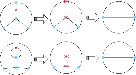
Figure 8. Graphical illustration of fatgraph edge removal▷ Top row. a regular edge ↼crossed↽ is removed from an $\mathcal{R}_{0,4}$ graph, its endpoints are further removed, the remaining edges are joined and the resulting graph is a trivalent fatgraph in $\mathcal{R}_{0,3}$▷ Bottom row. a loop is removed from a trivalent $\mathcal{R}_{0,4}$ graph, the stem together with its endpoints has to be removed as well, the remaining edges are joined⸦ and we end up with a trivalent fatgraph in $\mathcal{R}_{0,3}$▷

Case A↽. If $x$ is a loop attached to $v$⸦ then⸦ after deletion of $x$⸦ one needs to also delete the loose edge $x^{\prime}$ and the vertex $v^{\prime}$ ↼that is⸦ join the two other edges attached to $v^{\prime}$, see Figure 8⸦ bottom row↽▷ The resulting fatgraph $G^{\prime}$ has.

• two vertices less than $G$. $v$ and $v^{\prime}$ have been deleted,

• three edges less. $x$⸦ $x^{\prime}$ have been deleted and two other edges merged into one,

• one boundary cycle less. the boundary cycle totally bounded by $x$ has been removed▷

Therefore.

$$2-2g^{\prime} =\chi(G^{\prime})=l^{\prime}-m^{\prime}+n^{\prime}$$

$$=(l-2)-(m-3)+(n-1)$$

$$=l-m+n=\chi(G)=2-2g,$$

hence $g=g^{\prime}$⸦ and

$$G^{\prime}\in\mathcal{R}_{g,n-1}.$$ (A)

In case B↽⸦ $x$ joins distinct vertices $v$⸦ $v^{\prime}$ and separates distinct boundary cycles ↼see Figure 8⸦ top row↽▷ Delete $x$ and merge the two edges attached to each of the two vertices $v$ and $v^{\prime}$, in the process⸦ the two boundary cycles $\beta,\beta^{\prime}$ also merge into one▷ The resulting fatgraph $G^{\prime}$ is connected▷ Indeed⸦ given any two vertices $u,u^{\prime}\in V(G^{\prime})$⸦ there is a path $(x_{1},\ldots,x_{k})$ connecting $u$ with $u^{\prime}$ in $G$▷ If this path passes through $x$⸦ one can replace the occurrence of $x$ with the perimeter ⸧⸧⸧excluding $x$⸧⸧⸧ of one of the two boundary cycles $\beta,\beta^{\prime}$ to get a path joining $v$ and $v^{\prime}$ which avoids $x$⸦ and thus projects to a path in $G^{\prime}$▷ Again we see that $G^{\prime}$ has.

• two vertices less than $G$. $v$ and $v^{\prime}$ have been deleted,

• three edges less. $x$ has been deleted and four other edges merged into two⸦ pair by pair,

• one boundary cycle less. the boundary cycles $\beta$⸦ $\beta^{\prime}$ have been merged into one▷

Therefore $g=g^{\prime}$⸦ and

$$G^{\prime}\in\mathcal{R}_{g,n-1}.$$ (B)

In case C↽⸦ $x$ joins distinct vertices $v$⸦ $v^{\prime}$ but belongs into one boundary cycle $\beta\in B(G)$ only▷ Delete edge $x$ and the two vertices $v$⸦ $v^{\prime}$⸦ joining the attached edges two by two as in case B↽▷ We distinguish two cases⸦ depending on whether the resulting fatgraph is connected▷

1. If the resulting fatgraph $G^{\prime}$ is connected⸦ then $\beta\in B(G)$ has been split into two distinct boundary cycles $\beta^{\prime},\beta^{\prime\prime}\in B(G^{\prime})$▷ Indeed⸦ write the boundary cycle $\beta$ as an ordered sequence of oriented edges. $y_{0}\to y_{1}\to\ldots\to y_{k}\to y_{0}$▷ Assume the $y_{*}$ appear in this sequence in the exact order they are encountered when walking along $\beta$ in the sense given by the fatgraph orientation▷ The oriented edges $y_{i}$ are pairwise distinct. if $y_{i}$ and $y_{j}$ share the same supporting edge⸦ then $y_{i}$ and $y_{j}$ have opposite orientations▷ By the initial assumption of case C↽⸦ edge $x$ must appear twice in the list. if $\bar{x}$ and $\underline{x}$ denote the two orientations of $x$⸦ then $y_{i}=\bar{x}$ and $y_{j}=\underline{x}$▷ Deleting $x$ from $\beta$ is ↼from a homotopy point of view↽ the same as replacing $y_{i}=\bar{x}$ with $\bar{x}\to\underline{x}$⸦ and $y_{j}=\underline{x}$ with $\underline{x}\to\bar{x}$ when walking a boundary cycle▷ Then we see that $\beta$ splits into two disjoint cycles.

   $$\beta^{\prime} =y_{0}\to y_{1}\to\cdots\to y_{i-1}\to\bar{x}\to\underline{x}\to y_{j+1}\to\cdots\to y_{k}\to y_{0},$$

   $$\beta^{\prime\prime} =y_{i+1}\to\cdots\to y_{j-1}\to\underline{x}\to\bar{x}\to y_{i+1}.$$

   In this case⸦ $G^{\prime}$ has.

   • two vertices less than $G$. $v$ and $v^{\prime}$ have been deleted,

   • three edges less. $x$ has been deleted and four other edges merged into two⸦ pair by pair,

   • one boundary cycle more. the boundary cycle $\beta$ has been split in the pair $\beta^{\prime}$⸦ $\beta^{\prime\prime}$▷

   Therefore $g^{\prime}=g-1$ and $n^{\prime}=n+1$⸦ so.

   $$G^{\prime}\in\mathcal{R}_{g-1,n+1}.$$ (C’)

2. $G^{\prime}$ is a disconnected union of fatgraphs $G^{\prime}_{1}$ and $G^{\prime}_{2}$, for this statement to hold unconditionally⸦ we temporarily allow a single circle into the set of connected fatgraphs ↼consider it a fatgraph with one closed edge and no vertices↽ as the one and only element of $\mathcal{R}_{0,2}$▷ As will be shown in Lemma 5.2⸦ this is irrelevant for the MgnTrivalentGraphs algorithm▷ Now.

   $$l^{\prime}_{1}+l^{\prime}_{2}=l-2,\qquad m^{\prime}_{1}+m^{\prime}_{2}=m-3,\qquad n^{\prime}_{1}+n^{\prime}_{2}=n+1,$$

   hence.

   $$(2-2g^{\prime}_{1})+(2-2g^{\prime}_{2}) =(l-2)-(m-3)+(n+1)$$

   $$=(l-m+n)+2=4-2g$$

   So that $g^{\prime}_{1}+g^{\prime}_{2}=g+2$⸦ $n^{\prime}_{1}+n^{\prime}_{2}=n+1$⸦ and.

   $$G^{\prime}=G^{\prime}_{1}\otimes G^{\prime}_{2}\in\mathcal{R}_{g^{\prime}_{1},n^{\prime}_{1}}\otimes\mathcal{R}_{g^{\prime}_{2},n^{\prime}_{2}}.$$ (C”)

5▷1▷2 Inverse construction

If $x\in E(G)$ is an edge of a fatgraph $G$⸦ denote $\bar{x}$ and $\underline{x}$ the two opposite orientations of $x$▷

In the following⸦ let $\mathcal{R}^{\prime}_{g,n}$ be the set of fatgraphs with a selected oriented edge.

$$\mathcal{R}^{\prime}_{g,n}:=\{(G,\bar{x}):G\in\mathcal{R}_{g,n},\bar{x}\in L(G)\}.$$

Similarly⸦ let $\mathcal{R}^{\prime\prime}_{g,n}$ be the set of fatgraphs with two chosen oriented edges.

$$\mathcal{R}^{\prime\prime}_{g,n}:=\{(G,\bar{x},\bar{y}):G\in\mathcal{R}_{g,n},\bar{x},\bar{y}\in L(G)\}.$$

The following abbreviations are convenient.

$$\mathcal{R}=\cup\mathcal{R}_{g,n},\qquad\mathcal{R}^{\prime}=\cup\mathcal{R}^{\prime}_{g,n},\qquad\mathcal{R}^{\prime\prime}=\cup\mathcal{R}^{\prime\prime}_{g,n}.$$

Define the attachment of a new edge to a fatgraph in the following way▷ Given a fatgraph $G$ and an oriented edge $\bar{x}$⸦ we can create a new trivalent vertex $v$ in the midpoint of $x$⸦ and attach a new edge to it⸦ in such a way that the two halves of $x$ appear⸦ in the cyclic order at $v$⸦ in the same order induced by the orientation of $\bar{x}$▷ Figure 9 depicts the process▷

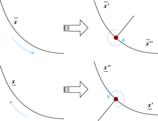
Figure 9. When adding a new vertex in the middle of an edge $x$⸦ the cyclic order depends on the oriented edge. the two orientations $\bar{x}$ and $\underline{x}$ get two inequivalent cyclic orders▷

We can now define maps that invert the constructions A↽⸦ B↽⸦ Cφ↽ and Cφφ↽ defined in the previous section▷

Figure 10. Graphical illustration of maps $p$⸦ $q$⸦ $r_{g,n}$▷ Top left. $p(G,\bar{x})$ attaches a ℓℓslipknotφφ to edge $\bar{x}$▷ Top right. $r_{2,5}(G_{1},\bar{x},G_{2},\bar{y})$ joins fatgraphs $G_{1}$ and $G_{2}$ with a new edge▷ Bottom. $q(G,\bar{x},\bar{y})$ ↼left↽ and $p(G,\underline{x},\bar{y})$ ↼right↽, it is shown how changing the orientation of an edge can lead to different results▷

Let $p_{g,n}:\mathcal{R}^{\prime}_{g,n-1}\to\mathcal{R}_{g,n}$ be the map that creates a fatgraph $p(G,\bar{x})$ from a pair $(G,\bar{x})$ by attaching the loose end of a ℓℓslip knotφφ to the midpoint of $x$▷ The map $p:\mathcal{R}^{\prime}\to\mathcal{R}$ defined by $p|_{\mathcal{R}^{\prime}_{g,n}}:=p_{g,n}$ is ostensibly inverse to A↽▷

To invert B↽ and Cφ↽⸦ define a map $q:\mathcal{R}^{\prime\prime}\to\mathcal{R}$ that operates as follows.

• Given $(G,\bar{x},\bar{y})$ with $\bar{x}\not=\bar{y}$⸦ the map $q$ attaches a new edge to the midpoints of $x$ and $y$, again the cyclic order on the new midpoint vertices is chosen such that the two halves of $x$ and $y$ appear in the order induced by the orientations $\bar{x}$⸦ $\bar{y}$▷

• When $\bar{x}=\bar{y}$⸦ let us further stipulate that the construction of $q(G,\bar{x},\bar{x})$ happens in two steps.

  1. a new trivalent vertex is created in the midpoint of $x\in E(G)$ and a new edge $\xi$ is attached to it⸦

  2. create a new trivalent vertex in the middle of the half⸧edge which comes first in the ordering induced by the orientation $\bar{x}$, attach the loose end of the new edge $\xi$ to this new vertex▷

  It is clear that the above steps give an unambiguous definition of $q$ in all cases where $\bar{x}$ and $\bar{y}$ are orientations of the same edge of $G$⸦ that is⸦ $(G,\bar{x},\bar{x})$⸦ $(G,\bar{x},\underline{x})$⸦ $(G,\underline{x},\bar{x})$⸦ and $(G,\underline{x},\underline{x})$▷

Ostensibly⸦ $q$ inverts the edge removal in cases B↽ and Cφ↽. the former applies when a graph $G\in\mathcal{R}_{g,n}$ is sent to $q(G)\in\mathcal{R}_{g,n+1}$⸦ the latter when $G\in\mathcal{R}_{g,n}$ is sent to $q(G)\in\mathcal{R}_{g+1,n-1}$▷

Finally⸦ to invert Cφφ↽⸦ let us define

$$r_{g,n}:\bigoplus_{\begin{subarray}{c}g^{\prime}_{1}+g^{\prime}_{2}=g+2\\ n^{\prime}_{1}+n^{\prime}_{2}=n\end{subarray}}\mathcal{R}^{\prime}_{g^{\prime}_{1},n^{\prime}_{1}}\times\mathcal{R}^{\prime}_{g^{\prime}_{2},n^{\prime}_{2}}\to\mathcal{R}.$$

From $(G^{\prime},\bar{x}^{\prime},G^{\prime\prime},\bar{x}^{\prime\prime})$⸦ construct a new fatgraph by bridging $G^{\prime}$ and $G^{\prime\prime}$ with a new edge⸦ whose endpoints are in the midpoints of $x^{\prime}$ and $x^{\prime\prime}$, again⸦ stipulate that the cyclic order on the new vertices is chosen such that the two halves of $x^{\prime}$⸦ $x^{\prime\prime}$ appear in the order induced by the orientations $\bar{x}^{\prime}$⸦ $\bar{x}^{\prime\prime}$▷

Summing up⸦ any fatgraph $G\in\mathcal{R}_{g,n}$ belongs to the image of one of the above maps $p$⸦ $q$⸦ and $r$▷ There is considerable overlap among the different image sets. in fact⸦ one can prove that $r$ is superfluous▷

Lemma 5▷2▷

Any fatgraph obtained by inverting construction Cφφ↽ lies in the image of maps $p$ and $q$▷

Proof▷

Assume⸦ on the contrarily⸦ that $G$ lies in the image of $r$ only▷ Then⸦ deletion of any edge $x$ from $G$ yields a disconnected graph $G^{\prime}\otimes G^{\prime\prime}$▷ Both subgraphs $G^{\prime}$ and $G^{\prime\prime}$ enjoy the same property⸦ namely⸦ that deletion of any edge disconnects. otherwise⸦ if the removal of $y\in E(G^{\prime})$ does not disconnect $G^{\prime}$⸦ then neither does it disconnect $G=r_{g,n}(G^{\prime},G^{\prime\prime})$⸦ contrary to the initial assumption▷ As long as $G^{\prime}$ or $G^{\prime\prime}$ has more than 3 edges⸦ we can delete another edge, by recursively repeating the process⸦ we end up with a fatgraph $G^{*}$ with $l^{*}\leqslant 3$ edges⸦ which is again disconnected by removal of any edge▷ Since $G^{*}$ is trivalent⸦ $3\cdot m^{*}=2\cdot l^{*}$⸦ therefore $G^{*}$ must have exactly 3 edges and 2 vertices▷ But all such fatgraphs belong to $\mathcal{R}_{0,3}$ or $\mathcal{R}_{1,1}$⸦ and it is readily checked that there is no way to add an edge such that the required property holds⸦ that any deletion disconnects▷ ∎

5▷1▷3 The MgnTrivalentGraphs algorithm

The stage is now set for implementing the recursive generation of trivalent graphs▷ Pseudo⸧code is listed in Algorithm 7▷

Algorithm 7 Return a list of all connected trivalent fatgraphs with prescribed genus $g$ and number of boundary cycles $n$▷ A fatgraph if ℓℓadmissibleφφ iff it has the prescribed genus $g$ and number of boundary cycles $n$▷

⬇

1def MgnTrivalentGraphs↼$g$⸦ $n$↽.

2 avoid infinite recursion in later statements

3 if $n$$=$ 0 or $(g,n)<(0,3)$.

4 return empty list

5

6 Induction base. $\mathcal{M}_{0,3}$ and $\mathcal{M}_{1,1}$

7 if $(g,n)$ $=$ $(0,3)$.

8 return list of fatgraphs in $\mathcal{R}_{0,3}$

9 elif $(g,n)$ $=$ $(1,1)$.

10 return list of fatgraphs in $\mathcal{R}_{1,1}$

11

12 general case

13 else.

14 R $\leftarrow$ empty list

15

16 case A↽. hang a circle to all edges of graphs in $M_{g,n-1}$

17 for $G$ in MgnTrivalentGraphs↼$g$⸦ $n-1$↽.

18 for $x$ in edge_orbits↼$G$↽.

19 add $p(G,\bar{x})$ toRif admissible

20 add $p(G,\underline{x})$ toRif admissible

21

22 case B↽. bridge all edges of a single graph in $M_{g,n-1}$

23 for $G$ in MgnTrivalentGraphs↼$g$⸦ $n-1$↽.

24 for $(x,y)$ in edge_pair_orbits↼$G$↽.

25 add $q(G,\underline{x},\underline{y})$ toRif admissible

26 add $q(G,\underline{x},\bar{y})$↽ toRif admissible

27 add $q(G,\bar{x},\underline{y})$ toRif admissible

28 add $q(G,\bar{x},\bar{y})$ toRif admissible

29

30 case C’↽. bridge all edges of a single graph in $M_{g-1,n+1}$

31 for $G$ in MgnTrivalentGraphs↼$g-1$⸦ $n+1$↽.

32 for $(x,y)$ in edge_pair_orbits↼$G$↽.

33 add $q(G,\underline{x},\underline{y})$ toRif admissible

34 add $q(G,\underline{x},\bar{y})$ toRif admissible

35 add $q(G,\bar{x},\underline{y})$ toRif admissible

36 add $q(G,\bar{x},\bar{y})$ toRif admissible

37

38 remove isomorphs from R

39 return R

Lemma 5▷3▷

MgnTrivalentGraphs$(g,n)$ generates all trivalent fatgraphs for each given $g$⸦ $n$▷ Only one representative per isomorphism class is returned▷

Proof▷

The function call MgnTrivalentGraphs$(g,n)$ recursively calls itself to enumerate trivalent graphs of $\mathcal{R}_{g,n-1}$ and $\mathcal{R}_{g-1,n+1}$▷ In particular⸦ MgnTrivalentGraphs must.

• provide the full set of fatgraphs $\mathcal{R}_{0,3}$ and $\mathcal{R}_{1,1}$ as induction base▷

• return the empty set when called with an invalid $(g,n)$ pair,

The general case is then quite straightforward. (1) apply maps $p$⸦ $q$ to every fatgraph in $\mathcal{R}_{g,n-1}$⸦ and $q$ to every fatgraph in $\mathcal{R}_{g-1,n+1}$, (2) discard all graphs that do not belong to $\mathcal{R}_{g,n}$, and (3) take only one graph per isomorphism class into the result set▷

To invert construction A↽⸦ map $p$ is applied to all fatgraphs $G\in\mathcal{R}_{g,n-1}$, if $a\in\operatorname{Aut}G$⸦ then $p(a(G),a(x))=p(G,x)$⸦ therefore we can limit ourselves to one pair $(G,x)$ per orbit of the automorphism group⸦ saving a few computational cycles▷ Similarly⸦ since $q$ is a function of $(G,\bar{x},\bar{y})$⸦ which is by construction invariant under $\operatorname{Aut}G$⸦ we can again restrict to considering only one $(G,\bar{x},\bar{y})$ per $\operatorname{Aut}G$⸧orbit, this is computed by the εedge_pair_orbits↼$G$↽ε function▷ ∎

Note that there is no way to tell from $G$ if fatgraphs $p(G,x)$ and $q(G,x,y)$ belong to $\mathcal{R}_{g,n}$. one needs to check $g$ and $n$ before adding the resulting fatgraph to the result set $R$▷

The selection of only one representative fatgraph per isomorphism class can be done by removing duplicates from the collection of generated graphs in the end⸦ or by running the isomorphism test before adding each graph to the working list $R$▷ The computational complexity is quadratic in the number of generated graphs in both cases⸦ but the latter option requires less memory▷ In any case⸦ this isomorphism test is the most computationally intensive part of MgnTrivalentGraphs▷

For an expanded discussion of the size of the result set $R$⸦ and a comparison with other generation algorithms⸦ see Appendix A▷ It would be interesting to re⸧implement the trivalent generation algorithm using the technique outlined in ♭mckay:isomorph-free♯⸦ and compare it with the current ↼rather naive↽ algorithm▷

5▷1▷4 Implementing maps $p(G,x)$ and $q(G,x,y)$

Implementation of both functions is straightforward and pseudo⸧code is therefore omitted, the only question is how to represent the ℓℓoriented edgesφφ that appear in the signature of maps $p$ and $q$▷

In both $p$ and $q$⸦ the oriented edge $\bar{x}$ or $\underline{x}$ is used to determine how to attach a new edge to the midpoint of the target ↼unoriented↽ edge $x$▷ We can thus represent an oriented edge as a pair $(\mathitbf{e},s)$ formed by a εFatgraphε edge $\mathitbf{e}$ and a ℓℓsideφφ $s$. valid values for $s$ are $+1$ and $-1$⸦ interpreted as follows▷ The parameter $s$ controls which of the two inequivalent cyclic orders the new trivalent vertex will be given▷ Let $\mathitbf{a}$⸦ $\mathitbf{b}$⸦ $\mathitbf{c}$ be the edges attached to the new vertex in the middle of $\mathitbf{e}$⸦ where $\mathitbf{a}$⸦$\mathitbf{b}$ are the two halves of $\mathitbf{e}$▷ If $s$ is $+1$⸦ then the new trivalent vertex will have the cyclic order $\mathitbf{a}<\mathitbf{b}<\mathitbf{c}<\mathitbf{a}$, if $s_{1}$ is $-1$⸦ then the edges $\mathitbf{a}$ and $\mathitbf{b}$ are swapped and the new trivalent vertex gets the cyclic order $\mathitbf{b}<\mathitbf{a}<\mathitbf{c}<\mathitbf{b}$ instead▷

6 The homology complex of marked fatgraphs

Betti numbers of a complex $(W_{*},D_{*})$ can be reckoned ↼via a little linear algebra↽ from the matrix form $\mathitbf{D}^{(k)}$ of the boundary operators $D_{k}$▷ Indeed⸦ given that $b_{k}:=\dim H_{k}(W,D)$ and $H_{k}(W,D):=Z_{k}(W,D)/B_{k}(W,D)=\operatorname{Ker}D_{k}/D_{k-1}(W_{k-1})$⸦ by the rank⸧nullity theorem we have $\dim\operatorname{Ker}D_{k}=\dim W_{k}-\operatorname{rank}\mathitbf{D}^{(k)}$ hence $b_{k}=\dim\operatorname{Ker}D_{k}-\dim D_{k-1}(W_{k-1})=\dim W_{k}-\operatorname{rank}\mathitbf{D}^{(k)}-\operatorname{rank}\mathitbf{D}^{(k-1)}$▷

In order to compute the matrix $\mathitbf{D}^{(k)}$⸦ we need to compute the coordinate vector of $D_{k}x^{(k)}_{j}$ for all vectors $x^{(k)}_{j}$ in a basis of $W_{k}$▷ If $(W_{*},D_{*})$ is the fatgraph complex⸦ then the basis vectors $x^{(k)}_{j}$ are marked fatgraphs with $k$ edges⸦ and the differential $D_{k}$ is defined as an alternating sum of edge contractions▷ Therefore⸦ in order to compute the coordinate vector of $D_{k}x^{(k)}_{j}$⸦ one has to find the unique fatgraph $x^{(k-1)}_{h}$ which is isomorphic to a given contraction of $x^{(k)}_{j}$ and score a $\pm 1$ coefficient depending on whether orientations agree or not▷

Although this approach works perfectly⸦ it is practically inefficient▷ Indeed⸦ lookups into the basis set $\{x^{(k-1)}_{h=1,\ldots,N}\}$ of $W_{k-1}$ require on average $O(N^{2})$ isomorphism checks▷ Still⸦ we can take a shortcut. if two topological fatgraphs $G$ and $G^{\prime}$ are not isomorphic⸦ so are any two marked fatgraphs $(G,\nu)$ and $(G^{\prime},\nu^{\prime})$▷ Indeed⸦ rearrange the rows and columns of the boundary operator matrix $\mathitbf{D}^{(k)}$ so that marked fatgraphs $(G,\nu)$ over the same topological fatgraph $G$ correspond to a block of consecutive indices▷ Then there is a rectangular portion of $\mathitbf{D}^{(k)}$ that is uniquely determined by a pair of topological fatgraphs $G$ and $G^{\prime}$▷ The main function for computing the boundary operator matrix can thus loop over pairs of topological fatgraphs⸦ and delegate computing the each rectangular block to specialized code▷ There are $n!/|\operatorname{Aut}G|$ marked fatgraphs per given topological fatgraph $G$⸦ so this approach can cut running time down by $O((n!)^{2})$▷

The generation of inequivalent marked fatgraphs ↼over the same topological fatgraph $G$↽ can be reduced to the ↼computationally easier↽ combinatorial problem of finding cosets of a subgroup of the symmetric group $\mathfrak{S}_{n}$▷ In addition⸦ the list of isomorphisms between $G$ and $G^{\prime}$ can be cached and re⸧used for comparing all pairs of marked fatgraphs $(G,\nu)$⸦ $(G^{\prime},\nu^{\prime})$▷ This strategy is implemented by two linked algorithms.

1. MarkedFatgraphPool. Generate all inequivalent markings of a given topological fatgraph $G$▷

2. compute_block. Given topological fatgraphs $G$ and $G^{\prime}$⸦ compute the rectangular block of a boundary operator matrix whose entries correspond to coordinates of $D(G,\nu)$ w▷r▷t▷ $(G^{\prime},\nu^{\prime})$▷

6▷1 Generation of inequivalent marked fatgraphs

For any marked fatgraph $(G,\nu)$⸦ denote $[G,\nu]$ its isomorphism class, recall that $B(-)$ is the functor associating a fatgraph with the set of its boundary cycles▷ Let $N(G)$ be the sets of all markings over $G$ and $\tilde{N}(G)$ the set of isomorphism classes thereof.

$$N(G) :=\{\,(G,\nu)\;|\;\nu\colon B(G)\to\{1,\ldots,n\}\,\},$$

$$\tilde{N}(G) :=\{\,[G,\nu]\;|\;\nu\colon B(G)\to\{1,\ldots,n\}\,\}.$$

Let $(G,\bar{\nu})$ be a chosen marked fatgraph▷ Define a group homomorphism.

$$\Phi:\operatorname{Aut}(G)\ni a\longmapsto\bar{\nu}\circ B(a)\circ\bar{\nu}^{-1}\in\mathfrak{S}_{n}.$$ (6)

The set $P=\Phi(\operatorname{Aut}G)$ is a subgroup of $\mathfrak{S}_{n}$▷

Lemma 6▷1▷

The marked fatgraphs $(G,\bar{\nu})$ and $(G,\sigma\bar{\nu})$ are isomorphic if and only if $\sigma\in P$▷

Proof▷

Let $\sigma\in P$⸦ then $\sigma^{-1}\in P$ and there exists $a\in\operatorname{Aut}G$ such that.

$$\sigma^{-1}=\bar{\nu}\circ B(a)\circ\bar{\nu}^{-1},$$

whence.

$$(\sigma\circ\bar{\nu})\circ B(a)\circ\bar{\nu}^{-1}=\operatorname{id},$$

therefore $a$ induces a marked fatgraph isomorphism between $(G,\bar{\nu})$ and $(G,\sigma\circ\bar{\nu})$▷

Conversely⸦ let $\hat{\nu}=\sigma\bar{\nu}$ and assume $(G,\bar{\nu})$ and $(G,\hat{\nu})$ are isomorphic as marked fatgraphs. then there exists $a\in\operatorname{Aut}G$ such that $\hat{\nu}\circ B(a)\circ\bar{\nu}^{-1}$ is the identity▷ Given any $\bar{\nu}\circ B(a^{\prime})\circ\bar{\nu}^{-1}\in P$ we have.

$$P\ni\bar{\nu}\circ B(a^{\prime})\circ\bar{\nu}^{-1}=\bar{\nu}\circ(\hat{\nu}^{-1}\circ\hat{\nu})\circ B(a)\circ B(a)^{-1}\circ B(a^{\prime})\circ\bar{\nu}^{-1}\\ =(\bar{\nu}\circ\hat{\nu}^{-1})\circ\hat{\nu}\circ B(a)\circ(\bar{\nu}^{-1}\circ\bar{\nu})\circ B(a^{-1})\circ B(a^{\prime})\circ\bar{\nu}^{-1}\\ =\sigma^{-1}\circ(\hat{\nu}\circ B(a)\circ\bar{\nu}^{-1})\circ\bar{\nu}\circ B(a^{-1}\circ a^{\prime})\circ\bar{\nu}^{-1}\\ =\sigma^{-1}\circ\left(\bar{\nu}\circ B(a^{-1}\circ a^{\prime})\circ\bar{\nu}^{-1}\right)\in\sigma^{-1}P,$$

therefore $P=\sigma^{-1}P$⸦ so $\sigma\in P$▷ ∎

Define a transitive action of $\mathfrak{S}_{n}$ over $N(G)$ by $\sigma\cdot(G,\nu):=(G,\sigma\nu)$, this descends to a transitive action of $\mathfrak{S}_{n}$ on $\tilde{N}(G)$▷ By the previous Lemma⸦ $P$ is the stabilizer of $[G,\bar{\nu}]$ in $\tilde{N}(G)$▷

Lemma 6▷2▷

The action of $\mathfrak{S}_{n}$ on $\tilde{N}(G)$ induces a bijective correspondence between isomorphism classes of marked fatgraphs and cosets of $P$ in $\mathfrak{S}_{n}$▷

Proof▷

Given isomorphic marked fatgraphs $(G,\nu)$ and $(G,\nu^{\prime})$⸦ let $\sigma,\sigma^{\prime}\in\mathfrak{S}_{n}$ be such that $\nu=\sigma\circ\bar{\nu}$ and $\nu^{\prime}=\sigma^{\prime}\circ\bar{\nu}$▷ By definition of marked fatgraph isomorphism⸦ there is $a\in\operatorname{Aut}G$ such that the following diagram commutes.

$$\xymatrix{B(G)&B(G)\\ \{1,\ldots,n\}\ar^{B(a)}"1,1";"1,3"\ar_{\sigma\circ\bar{\nu}=\nu}"1,1";"2,2"\ar^{\nu^{\prime}=\sigma^{\prime}\circ\bar{\nu}}"1,3";"2,2"}$$

Hence commutativity of another diagram follows.

$$\xymatrix{B(G)&B(G)\\ \{1,\ldots,n\}\{1,\ldots,n\}\ar^{B(a)}"1,1";"1,3"\ar_{\bar{\nu}}"1,1";"2,1"\ar^{\bar{\nu}}"1,3";"2,3"\ar_{\sigma^{-1}\sigma^{\prime}}"2,3";"2,1"}$$

Thus $(G,\bar{\nu})$ is isomorphic to $(G,\sigma^{-1}\sigma^{\prime}\circ\bar{\nu})$, therefore $\sigma^{-1}\sigma^{\prime}\in P$⸦ hence⸦ $\sigma^{\prime}\in\sigma P$⸦ i▷e▷⸦ $\sigma$ and $\sigma^{\prime}$ belong into the same coset of $P$▷

Conversely⸦ let $\tau,\tau^{\prime}\in\sigma P$, explicitly.

$$\tau=\sigma\circ\bar{\nu}\circ B(a)\circ\bar{\nu}^{-1},\qquad\tau^{\prime}=\sigma\circ\bar{\nu}\circ B(a^{\prime})\circ\bar{\nu}^{-1}.$$

Set $\nu=\tau\circ\bar{\nu}$⸦ $\nu^{\prime}=\tau^{\prime}\circ\bar{\nu}$, substituting back the definition of $\tau$⸦ we have.

$$\nu=\sigma\circ\bar{\nu}\circ B(a)\circ\bar{\nu}^{-1}\circ\bar{\nu}=\sigma\circ\bar{\nu}\circ B(a),$$

whence $\bar{\nu}=\sigma^{-1}\circ\nu\circ B(a)^{-1}$⸦ and.

$$\nu^{\prime}=\sigma\circ\bar{\nu}\circ B(a^{\prime})=\sigma\circ\left(\sigma^{-1}\circ\nu\circ B(a)^{-1}\right)\circ B(a^{\prime})=\nu\circ B(a^{-1}\circ a^{\prime}),$$

therefore $a^{-1}\circ a^{\prime}$ is an isomorphism between the marked fatgraphs $(G,\nu)$ and $(G,\nu^{\prime})$▷ ∎

The following is an easy corollary of the transitivity of the action of $\mathfrak{S}_{n}$ on $\tilde{N}(G)$▷

Lemma 6▷3▷

Given any marking $\nu$ on the fatgraph $G$⸦ there exist $\sigma\in\mathfrak{S}_{n}$ and $a\in\operatorname{Aut}G$ such that. $\nu=\sigma\circ\bar{\nu}\circ a$▷

Proof▷

By Lemma 6.2⸦ there exists $\sigma\in\mathfrak{S}_{n}$ such that $[G,\nu]=[G,\sigma\circ\bar{\nu}]$⸦ i▷e▷⸦ $(G,\nu)$ is isomorphic to $(G,\sigma\circ\bar{\nu})$▷ If $a\in\operatorname{Aut}G$ is this fatgraph isomorphism⸦ then the following diagram commutes.

$$\xymatrix{B(G)&B(G)\\ \{1,\ldots,n\}\ar^{B(a)}"1,1";"1,3"\ar_{\nu}"1,1";"2,2"\ar^{\sigma\circ\bar{\nu}}"1,3";"2,2"}$$

Therefore $\nu=\sigma\circ\bar{\nu}\circ B(a)$▷ ∎

The MarkedFatgraphPool algorithm▷

Given a fatgraph $G$ and a εFatgraphε object ε$\mathitbf{G}$ε representing it⸦ let us stipulate that $\bar{\nu}$ be the marking on $G$ that enumerates boundary cycles of $G$ in the order they are returned by the function εcompute_boundary_cycles↼$\mathitbf{G}$↽ε▷ By Lemma 6.3⸦ every $(G,\nu^{(j)})$ can then be expressed ↼up to isomorphism↽ as $(G,\sigma^{(j)}\circ\bar{\nu})$ with $\sigma^{(j)}\in\mathfrak{S}_{n}$▷ The set $\{\sigma^{(j)}\}$ enumerates all distinct isomorphism classes of marked fatgraphs over $G$ iff $\{\sigma^{(j)}P\}$ runs over all distinct cosets of $P$ in $\mathfrak{S}_{n}$ ↼by Lemma 6.2↽▷

The εMarkedFatgraphPoolε function computes the set $\tilde{N}(G)$ of isomorphism classes $[G,\nu]$▷

Theorem 6▷1▷

Given a εFatgraphε $\mathitbf{G}$ as input⸦ the output of εMarkedFatgraphPool↼$\mathitbf{G}$↽ε⸦ as computed by Algorithm 8⸦ is a tuple ε↼graph⸦ $P$⸦ $A$⸦ markings⸦ orientable↽ε⸦ whose components are defined as follows.

• The εgraphε item is the underlying εFatgraphε object ε$\mathitbf{G}$ε▷

• The ε$P$ε slot holds a list of all elements in the group $P=\Phi(\operatorname{Aut}G)$▷

• A corresponding set of pre⸧image representatives ↼each element is an automorphism of ε$\mathitbf{G}$ε↽ is stored into ε$A$ε. permutation ε$P[i]$ε is induced by automorphism ε$A[i]$ε⸦ i▷e▷⸦ if $\pi=P[i]$ and $a=A[i]$ then $\pi=\Phi(a)$▷

• The εmarkingsε item holds the list $\{\sigma^{(j)}\}$ of distinct cosets of $P$ ↼representing inequivalent markings↽▷

• εorientableε is a boolean value indicating whether any $(G,\nu)$ in the pool is orientable▷

We need a separate boolean variable to record the orientability of the family of marked fatgraphs $N(G)=\{(G,\nu)\}$⸦ because the automorphism group of a marked fatgraph $\operatorname{Aut}(G,\nu)$ can be a proper subgroup of $\operatorname{Aut}G$. hence⸦ $(G,\nu)$ can be orientable even if $G$ is not▷

Algorithm 8 Compute the distinct markings of a given fatgraph▷ Input to the algorithm is a Fatgraph object $\mathitbf{G}$, final result is a tuple ↼$\mathitbf{G}$⸦ $P$⸦ $A$⸦ markings⸦ orientable↽ which represents the set $\tilde{N}(G)$ of isomorphism classes of marked fatgraphs▷

⬇

1def phi↼$a$⸦ $\mathitbf{G}$↽.

2 $\pi$ $\leftarrow$ array of $n$ elements

3 for src_index⸦ src_cycle in enumerate↼$\mathitbf{G}$▷boundary_cycles↽.

4 dst_cycle $\leftarrow$ $a$▷transform_boundary_cycle↼src_cycle↽

5 if dst_cycle not in $\mathitbf{G}$▷boundary_cycles.

6 abort and signal error to caller

7 else.

8 dst_index $\leftarrow$ index ofdst_cyclein$\mathitbf{G}$▷boundary_cycles

9 $\pi$♭src_index♯ $\leftarrow$ dst_index

10 return $\pi$

11

12def MarkedFatgraphPool↼$\mathitbf{G}$↽.

13 P $\leftarrow$ empty list

14 A $\leftarrow$ empty list

15 assume $(G,\nu)$ is orientable until we have counter⸧evidence

16 orientable $\leftarrow$ True

17 step ↼1↽. loop over $\operatorname{Aut}G$

18 for $a$ in $\mathitbf{G}$▷automorphisms↼↽.

19 try.

20 $\pi$ $\leftarrow$ phi↼$a$⸦ $\mathitbf{G}$↽

21 except phi failed.

22 continue with next$a$

23 if permutation$\pi$is identity.

24 found a new automorphism.

25 ⸧ does it reverse orientation⋆

26 if $a$▷is_orientation_reversing↼↽.

27 orientable $\leftarrow$ False

28 ⸧ does it define a new marking⋆

29 if $\pi$ not in P.

30 append$\pi$to $P$

31 append$a$to $A$

32 step ↼2↽. enumerate cosets of $P$

33 markings $\leftarrow$ ♭ ♯

34 for $\sigma$ in $\mathfrak{S}_{n}$.

35 for $\pi$ in $P$.

36 if $\pi\circ\sigma$ in markings.

37 continue with next $\sigma$

38 add $\sigma$ tomarkings

Proof▷

Generation of all inequivalent markings over $G$ is a direct application of Lemma 6.2⸦ performed in two steps.

1. In the first step⸦ for each automorphism $a\in\operatorname{Aut}G$ compute the permutation $\Phi(a)$ it induces on the set of boundary components⸦ and form the subgroup $P$▷ The subgroup $P$ and the associated set of automorphisms $A\subseteq\operatorname{Aut}G$ are stored in variables εPε and εAε▷

2. In the second step⸦ compute cosets of $P$ by exhaustive enumeration▷ They are recast into the list $\{\sigma^{(j)}\}$⸦ which is stored into the εmarkingsε variable▷

As an important by⸧product of the computation⸦ the automorphism group $\operatorname{Aut}(G,\bar{\nu})$ is computed⸦ and used to determine if the marked fatgraphs in the pool are orientable▷

The auxiliary function phi computes the permutation $\Phi(a)=\bar{\nu}\circ B(a)\circ\bar{\nu}^{-1}$▷ A permutation ε$\pi$ε is created and returned, it is represented by an array with $n$ slots⸦ which is initially empty and is then stepwise constructed by iterating over boundary cycles▷ Indeed⸦ the boundary cycle εsrc_cycleε is transformed according to $B(a)$ and its position in the list of boundary cycles of $\mathitbf{G}$ is then looked up▷ Note that this lookup may fail. there are in fact cases⸦ in which the Fatgraph▷isomorphisms algorithm finds a valid mapping⸦ that however does not preserve the markings on boundary cycles, such failures need to be dealt with by rejecting $a$ as a εFatgraphε automorphism▷

Step ↼1↽ of the computation is performed in lines 18⸧⸧27.

• Computation of the permutation $\pi$ ↼induced by $a$ on the boundary cycles of $\mathitbf{G}$↽ may fail, if this happens⸦ the algorithm ignores $a$ and proceeds with another automorphism▷

• If $a$ preserves the boundary cycles pointwise⸦ then it induces an automorphism of the marked graph and we need to test whether it preserves or reverses orientation▷

• There are $\lvert\operatorname{Ker}\Phi\rvert$ distinct automorphisms inducing the same permutation on boundary cycles. if ε$\pi$ε is already in $P$⸦ discard it and continue with the next $a$▷

By Lemma 6.2⸦ there are as many distinct markings as there are cosets of εPε in $\mathfrak{S}_{n}$▷ Step ↼2↽ of the algorithm proceeds by simply enumerating all permutations in $\mathfrak{S}_{n}$⸦ with εmarkingε initially set to the empty list, for each permutation $\sigma$ a test is made as to whether $\sigma P$ intersects the list εmarkingsε ↼lines 35⸧⸧37↽, if it does not⸦ then the marking induced by $\sigma$ is added to the list▷

∎

A constructive version of Lemma 6.3 can now be implemented. the following function index_and_aut⸦ given a εFatgraphε object $\mathitbf{G}$ and a marking⸦ returns the permutation ↼by index number ε$j$ε in ε$\mathitbf{G}$▷markingsε↽ and fatgraph automorphism $a=\mathitbf{G}.A[i]$ such that the topological fatgraph ε$\mathitbf{G}$ε decorated with εmarkingε is isomorphic ↼through $a$↽ to the same graph decorated with ε$\mathitbf{G}$▷markings♭$j$♯ε▷

⬇

1def index_and_aut↼$\mathitbf{G}$⸦ marking↽.

2 for $(i,\pi)$ in enumerate↼$\mathitbf{G}.P$↽.

3 $\tau$ $\leftarrow$ $\sigma\circ\pi$

4 if $\tau$ in $\mathitbf{G}$▷markings.

5 $j$ $\leftarrow$ index of $\tau$ in$\mathitbf{G}$▷markings

6 return $(j,\mathitbf{G}.A[i])$

7 else.

8 continue with next $\pi$

The algorithm enumerates all permutations $\pi\in P$⸦ and compares $\sigma\circ\pi$ to every element of ε$\mathitbf{G}$▷markingsε. by Lemma 6.2⸦ we know that one must match▷

6▷2 Computing boundary operator matrix blocks

The differential $D(G,\nu)$ is computed by summing contractions of regular edges in $G$ ↼with alternating signs↽, likewise⸦ the matrix block corresponding to coordinates of the families of marked fatgraphs $\{(G,\nu)\}$ and $\{(G^{\prime},\nu^{\prime})\}$ can be decomposed into a sum of blocks⸦ each block representing the coordinates of $\{(G/e,\nu)\}_{e\in E(G)}$ projected on the linear span of $\{(G^{\prime},\nu^{\prime})\}$▷

More precisely⸦ given any two fatgraphs $G_{1}$ ↼with $m$ edges↽ and $G_{2}$ ↼with $m-1$ edges↽⸦ let $X_{1},X_{2}\subseteq\mathscr{R}_{g,n}$ be the linear span of $N(G_{1})$ and $N(G_{2})$ respectively⸦ and denote by $\mathrm{pr}_{X_{2}}$ the linear projection on subspace $X_{2}$▷ Recall that⸦ for any fatgraph $G$⸦ we have $D(G)=\sum\pm d^{(e)}(G)$⸦ where the sum is taken over all regular edges $e$ of $G$⸦ and $d^{(e)}$ is the contraction of edge $e$▷

Let $G$ be the fatgraph obtained by contracting the chosen edge $e$ in $G_{1}$▷ If $G_{2}$ and $G$ are isomorphic⸦ then the three graphs are related by the following diagram of fatgraph morphisms⸦ where $f_{1}$ is the contraction map and $f_{2}$ is a fatgraph isomorphism.

$$\xymatrix{G_{1}&\\ GG_{2}\ar_{f_{1}}"1,1";"2,1"\ar_{f_{2}}^{\sim}"2,1";"2,2"}$$ (7)

The above diagram (7) functorially induces a diagram on the set of boundary cycles.

$$\xymatrix{B(G_{1})&\{1,\ldots,n\}\\ B(G)B(G_{2})\ar_{B(f_{1})}^{=}"1,1";"2,1"\ar_{B(f_{2})}^{\sim}"2,1";"2,2"\ar^{\nu_{1}}"1,1";"1,2"\ar_{\nu}"2,1";"1,2"\ar_{\nu_{2}}"2,2";"1,2"}$$ (8)

Diagram (8) commutes iff $f_{1}$⸦ $f_{2}$ can be extended to morphisms of marked fatgraphs $\hat{f}_{1}:(G_{1},\nu_{1})\to(G,\nu)$ and $\hat{f}_{2}:(G,\nu)\to(G_{2},\nu_{2})$▷

Now choose εFatgraphε objects $\mathitbf{G}_{1}$⸦ $\mathitbf{G}$⸦ $\mathitbf{G}_{2}$ representing $G_{1}$⸦ $G$⸦ $G_{2}$▷

Let $\bar{\nu}_{1}$⸦ $\bar{\nu}$⸦ $\bar{\nu}_{2}$ be the markings on $G_{1}$⸦ $G$⸦ $G_{2}$ that enumerate boundary cycles in the order they are returned by the function εcompute_boundary_cycleε applied to ε$\mathitbf{G}_{1}$ε⸦ ε$\mathitbf{G}$ε⸦ ε$\mathitbf{G}_{2}$ε respectively▷ Define $\phi_{1},\phi_{2}\in\mathfrak{S}_{n}$ by.

$$\phi_{1}:=\bar{\nu}\circ B(f_{1})\circ\bar{\nu}_{1}^{-1},\qquad\phi_{2}:=\bar{\nu}_{2}\circ B(f_{2})\circ\bar{\nu}^{-1}.$$ (9)

Lemma 6▷4▷

Given any marking $\nu_{1}$ on $G_{1}$⸦ choose $\sigma_{1}\in\mathfrak{S}_{n}$ such that $\nu_{1}=\sigma_{1}\circ\bar{\nu}_{1}$ and define.

$$\nu_{2}:=\sigma_{1}\circ\phi_{1}^{-1}\circ\phi_{2}^{-1}\circ\bar{\nu}_{2},$$ (10)

Then $\nu_{2}$ is the unique marking on $G_{2}$ such that diagram (8) commutes▷

Proof▷

Let $\sigma_{2}:=\sigma_{1}\circ\phi_{1}^{-1}\circ\phi_{2}^{-1}$▷ We need to prove that the external square in diagram (8) is commutative, indeed⸦ we have.

$$\sigma_{2}=\sigma_{1}\circ(\bar{\nu}_{1}\circ B(f_{1})^{-1}\circ\bar{\nu}^{-1})\circ(\bar{\nu}\circ B(f_{2})^{-1}\circ\bar{\nu}_{2})\\ =\sigma_{1}\bar{\nu}_{1}\circ B(f_{2}\circ f_{1})^{-1}\circ\bar{\nu}_{2}^{-1},$$

so that.

$$\nu_{2}\circ B(f_{2})\circ B(f_{1})=\sigma_{2}\circ\nu_{2}\circ B(f_{2}\circ f_{1})\\ =\sigma_{1}\bar{\nu}_{1}\circ B(f_{2}\circ f_{1})^{-1}\circ\bar{\nu}_{2}^{-1}\circ\nu_{2}\circ B(f_{2}\circ f_{1})\\ =\sigma_{1}\circ\bar{\nu}_{1}=\nu_{1}.$$

The uniqueness assertion is of immediate proof⸦ since maps $B(f_{1})$ and $B(f_{2})$ are invertible▷ ∎

Let $\mathitbf{p}_{1}$⸦ $\mathitbf{p}_{2}$ be the εMarkedFatgraphPoolε output corresponding to $\mathitbf{G}_{1}$⸦ $\mathitbf{G}_{2}$⸦ and let $\{\nu_{1}^{(j)}\}_{j=1,\ldots,N_{1}}$⸦ $\{\nu_{2}^{(k)}\}_{k=1,\ldots,N_{2}}$ be the enumeration of fatgraph markings corresponding to items in the lists ε$\mathitbf{p}_{1}$▷markingsε and ε$\mathitbf{p}_{2}$▷markingsε respectively▷

Lemma 6▷5▷

For any regular edge $e$ of $G_{1}$⸦ and any choice of $j\in\{1,\ldots,N_{1}\}$⸦ there exist unique $k\in\{1,\ldots,N_{2}\}$ and $s\in\{-1,0,+1\}$ such that.

$$\mathrm{pr}_{X_{2}}\left(d^{(e)}[G_{1},\nu_{1}^{(j)}]\right)=s\cdot[G_{2},\nu_{2}^{(k)}].$$ (11)

Proof▷

If $G_{2}$ and $G=G_{1}/e$ are not isomorphic⸦ then⸦ for any marking $\nu_{1}$⸦ $d(G_{1},\nu_{1})$ has no component in the subspace $X_{2}=\{(G_{2},\nu_{2})\}$⸦ so the assertion is true with $s=0$▷

Otherwise⸦ by Lemma 6.4⸦ given $\nu_{1}=\nu_{1}^{(j)}$ there is a unique $\nu_{2}$ such that $s$ can be non⸧null, by Lemma 6.3⸦ there exist $\nu_{2}^{(k)}:=\sigma_{2}^{(k)}\circ\bar{\nu}_{2}$ and $a\in\operatorname{Aut}G$ such that.

1. the marked fatgraph $(G_{2},\nu_{2}^{(k)})$ is a representative of the isomorphism class $[G_{2},\nu_{2}]$,

2. $a$ gives the isomorphism between marked fatgraphs $(G_{2},\nu_{2})$ and $(G_{2},\nu_{2}^{(k)})$,

3. $\nu_{2}^{(k)}$ is the marking on $G_{2}$ represented by $k$⸧th item in list ε$\mathitbf{p}_{2}$▷markingsε▷

The coefficient $s$ must then be $\pm 1$ since both $(G_{2},\nu_{2}^{(k)})$ and $d^{(e)}(G_{1},\nu_{1}^{(j)})$ are ↼isomorphic to↽ elements in the basis of $X_{2}$▷ ∎

Theorem 6▷2▷

Given εMarkedFatgraphPoolε objects $\mathitbf{p}_{1}$⸦ $\mathitbf{p}_{2}$⸦ and a chosen edge $\mathitbf{e}$ of $\mathitbf{G}_{1}$⸦ the function εcompute_blockε in Algorithm 9 returns the set $S$ of all triplets $(j,k,s)$ with $s=\pm 1$ such that.

$$\mathrm{pr}_{X_{2}}\left(d^{(e)}[G_{1},\nu_{1}^{(j)}]\right)=s\cdot[G_{2},\nu_{2}^{(k)}].$$ (12)

Algorithm 9 Return the set $S$ of triplets $(j,k,s)$ such that eq▷ (12) holds for $(G_{1},\nu_{1}^{(j)})$ and $(G_{2},\nu_{2}^{(k)})$ obtained by contracting $\mathitbf{e}$ in all marked graphs in $\mathitbf{p}_{1}$ and projecting onto graphs in the $\mathitbf{p}_{2}$ family▷

⬇

1def compute_block↼$\mathitbf{p}_{1}$⸦ $\mathitbf{e}$⸦ $\mathitbf{p}_{2}$↽.

2 $\mathitbf{G}_{1}$ $\leftarrow$ $\mathitbf{p}_{1}$▷graph

3 $\mathitbf{G}_{2}$ $\leftarrow$ $\mathitbf{p}_{2}$▷graph

4 $\mathitbf{G}$ $\leftarrow$ contract↼$\mathitbf{G}_{1}$⸦ $\mathitbf{e}$↽

5 if $\mathitbf{G}$ and $\mathitbf{G}_{2}$ are not isomorphic.

6 return empty list

7 else.

8 result $\leftarrow$ empty list

9 $\mathitbf{f}_{2}$ $\leftarrow$ first isomorphism computed byFatgraph▷isomorphisms↼$\mathitbf{G}$⸦ $\mathitbf{G}_{2}$↽

10 $\phi_{1}^{-1}$ $\leftarrow$ compute_phi1_inv↼$\mathitbf{G}$⸦ $\mathitbf{G}_{1}$⸦ $\mathitbf{e}$↽

11 $\phi_{2}^{-1}$ $\leftarrow$ compute_phi2_inv↼$\mathitbf{G}$⸦ $\mathitbf{G}_{2}$⸦ $\mathitbf{f}_{2}$↽

12 for $(j,\sigma)$ in enumerate↼$\mathitbf{p}_{1}$▷markings↽.

13 $(k,\mathitbf{a})$ $\leftarrow$ index_and_aut↼$\mathitbf{p}_{2}$⸦ $\sigma\circ\phi_{1}^{-1}\circ\phi_{2}^{-1}$↽

14 $p$ $\leftarrow$ $\mathitbf{G}_{1}$▷orient♭$\mathitbf{e}$♯

15 $s$ $\leftarrow$ $(-1)^{p}$ * compare_orientations↼$\mathitbf{f}_{2}$↽ * compare_orientations↼$\mathitbf{a}$↽

16 append $(j,k,s)$ toresult

17 return result

18

19def compute_phi1_inv↼$\mathitbf{G}$⸦ $\mathitbf{G}_{1}$⸦ $\mathitbf{e}$↽.

20 $\tau$ $\leftarrow$ empty array of $n$ elements

21 for $i$⸦ $\mathitbf{b}$ in enumerate↼$\mathitbf{G}_{1}$▷boundary_cycles↽.

22 $\mathitbf{b}^{\prime}$ $\leftarrow$ contract_boundary_cycle↼$\mathitbf{G}_{1}$⸦ $\mathitbf{b}$⸦ $\mathitbf{e}$↽

23 $i^{\prime}$ $\leftarrow$ index of $\mathitbf{b}^{\prime}$ in$\mathitbf{G}$▷boundary_cycles

24 $\tau[i^{\prime}]$ $\leftarrow$ $i$

25 return $\tau$

26

27def compute_phi2_inv↼$\mathitbf{G}$⸦ $\mathitbf{G}_{2}$⸦ $f_{2}$↽.

28 $\tau^{\prime}$ $\leftarrow$ empty array of $n$ elements

29 for $i$⸦ $\mathitbf{b}$ in enumerate↼$\mathitbf{G}_{2}$▷boundary_cycles↽.

30 $\mathitbf{b}^{\prime}$ $\leftarrow$ transform_boundary_cycle↼$f_{2}$⸦ $\mathitbf{b}$↽

31 $i^{\prime}$ $\leftarrow$ index of $\mathitbf{b}^{\prime}$ in$\mathitbf{G}$▷boundary_cycles

32 $\tau^{\prime}[i^{\prime}]$ $\leftarrow$ $i$

33 return $\tau^{\prime}$

Proof▷

The algorithm closely follows the computation done before Lemmas 6.4 and in the proof of Lemma 6.5▷

If $G_{2}$ and $G=G_{1}/e$ are not isomorphic⸦ then $d^{(e)}[G_{1},\nu_{1}]$ has no component in the subspace $X_{2}$ generated by $\{[G_{2},\nu_{2}]\}$⸦ whatever the marking $\nu_{1}$▷ The assertion is thus satisfied by $S=\varnothing$⸦ i▷e▷⸦ an empty list of triplets $(j,k,s)$ ↼lines 5⸧⸧6 in Algorithm 9↽▷

If $G_{2}$ is isomorphic to $G=G_{1}/e$ through $f_{2}$⸦ then Lemma 6.4 provides the explicit formula $\nu_{2}^{(k)}=\sigma_{1}^{(j)}\circ\phi_{1}^{-1}\circ\phi_{2}^{-1}\circ\bar{\nu}_{2}$⸦ where $\sigma_{1}^{(j)}=\nu_{1}^{(j)}\circ\bar{\nu}_{1}^{-1}$▷

By assumption⸦ $\bar{\nu}_{1}$ numbers the boundary cycles on $G_{1}$ in the order they are returned by running function εcompute_boundary_cyclesε on $\mathitbf{G}_{1}$⸦ so $\sigma_{1}^{(j)}$ is the permutation corresponding to the $j$⸧th element in ε$\mathitbf{p}_{1}$▷markingsε▷

The map $\phi_{1}$ is easy to compute. again⸦ given that both $\bar{\nu}$ and $\bar{\nu}_{1}$ number the boundary cycles of $G$ and $G_{1}$ in the order they are returned by εcompute_boundary_cyclesε⸦ the auxiliary function εcompute_phi1_invε incrementally builds the result by looping over ε$\mathitbf{G}_{1}$▷boundary_cyclesε⸦ contracting the target edge⸦ and mapping the corresponding indices▷

Computation of the map $\phi_{2}$ depends on the isomorphism $f_{2}$, however⸦ two different choices for $f_{2}$ will not change the outcome of the algorithm. in the final loop at lines 12⸧⸧16⸦ only the sign of $f_{2}$ is used⸦ and the sign is constant across all isomorphisms having the same source and target fatgraphs ↼iff they are both orientable↽▷ Computation of $\phi_{2}^{-1}$ ↼in the auxiliary function εcompute_phi2_invε↽ is done in the same way as the computation of $\phi_{1}^{-1}$⸦ except we transform $b$ to $b^{\prime}$ by means of εtransform_boundary_cycle↼$f_{2}$⸦ $-$↽ε⸦ i▷e▷⸦ $B(f_{2})$▷

Finally⸦ for every marking ε$\sigma_{1}^{(j)}$ε in ε$\mathitbf{p}_{1}$▷markingsε ↼representing $\nu_{1}^{(j)}$↽⸦ we know by Lemma 6.5 that there is a unique index $k$ and $a\in\operatorname{Aut}G_{2}$ such that. $\sigma_{1}^{(j)}\circ\phi_{1}^{-1}\circ\phi_{2}^{-1}=\sigma_{2}^{(k)}$ is the $k$⸧th item in ε$\mathitbf{p}_{2}$▷markingsε ↼representing $\nu_{2}^{(k)}$↽⸦ and such that the following chain.

$$\xymatrix{G_{1}&GG_{2}G_{2}\ar_{f_{1}}"1,1";"1,2"\ar_{f_{2}}^{\simeq}"1,2";"1,3"\ar_{a}^{\simeq}"1,3";"1,4"}$$

extends to a marked fatgraph morphism.

$$\xymatrix{(G_{1},\nu_{1}^{(j)})&(G,\nu)(G_{2},\nu_{2})(G_{2},\nu_{2}^{(k)}).\ar_{\hat{f}_{1}}"1,1";"1,2"\ar_{\hat{f}_{2}}^{\simeq}"1,2";"1,3"\ar_{\hat{a}}^{\simeq}"1,3";"1,4"}$$

The sign $s$ is then obtained by comparing the orientation $\omega_{2}$ of $(G_{2},\nu_{2}^{(k)})$ with the push⸧forward orientation ${(a\circ f_{2}\circ f_{1})}_{*}\omega_{1}$⸦ where $\omega_{1}$ is the orientation on $(G_{1},\nu_{1}^{(j)})$⸦ and multiplying by the alternating sign from the homology differential▷ There are four components that make up $s$.

• the sign given by the contraction $f_{1}$. this is $+1$ by definition since the ℓℓchildφφ fatgraph $G$ inherits the orientation from the ℓℓparentφφ fatgraph $G_{1}$,

• the sign given by the isomorphism $f_{2}$. this is obtained by comparing $(f_{2})_{*}\omega$ with $\omega_{2}$⸦ which is implemented for a generic isomorphism by the function εcompare_orientationsε,

• the sign of the automorphism $a$ of ε$G_{2}$ε which transforms the push⸧forward marking into the chosen representative in the same orbit. this again can be computed by comparing $(a)_{*}\omega_{2}$ with $\omega_{2}$ and only depends on the action of $a$ on edges of $G_{2}$,

• the alternating sign from the homology differential⸦ which only depends on the position $p$ of edge $e$ within the order $\omega_{1}$▷

The product of the three non⸧trivial components is returned as the sign $s$ ↼line 15↽▷ ∎

6▷3 Matrix form of the differential $D$

The εcompute_boundary_operatorsε function ↼Algorithm 10↽ computes the matrix form $\mathitbf{D}^{(m)}$ of the differential $D$ restricted to the linear space generated by fatgraphs with $m$ edges▷

Input to the function are the number $m$ and the list of graphs⸦ divided by number of fatgraph edges. εgraphs♭$m$♯ε is the list of fatgraphs with $m$ edges▷

The output matrix $\mathitbf{D}^{(m)}$ is constructed incrementally. it starts with all entries set to $0$⸦ and is then populated blockwise▷ Indeed⸦ for every pair of εMarkedFatgraphPoolε objects $\mathitbf{p}_{1}$ ↼from a graph with $m$ edges↽ and $\mathitbf{p}_{2}$ ↼with $m-1$ edges↽⸦ and every non⸧loop edge $\mathitbf{e}$⸦ the rectangular matrix block whose upper⸧left corner is at indices $j_{0},k_{0}$ is summed the block resulting from εcompute_block↼$\mathitbf{p}1$⸦ $\mathitbf{e}$⸦ $\mathitbf{p}_{2}$↽ε▷

Algorithm 10 Compute the boundary operator matrix⸦ block by block▷

⬇

1def compute_boundary_operator↼$m$⸦ graphs↽.

2 $N_{1}$ $\leftarrow$ number of graphs with $m$ edges

3 $N_{2}$ $\leftarrow$ number of graphs with $m-1$ edges

4 $D^{(m)}$ $\leftarrow$ $N_{1}\times N_{2}$ matrix⸦ initially null

5 $j_{0}$ $\leftarrow$ 0

6 for $\mathitbf{G}_{1}$ in graphs♭m♯.

7 $\mathitbf{p}_{1}$ $\leftarrow$ MarkedFatgraphPool↼$\mathitbf{G}_{1}$↽

8 $k_{0}$ $\leftarrow$ 0

9 for $\mathitbf{G}_{2}$ in graphs♭m⸧1♯.

10 $\mathitbf{p}_{2}$ $\leftarrow$ MarkedFatgraphPool↼$\mathitbf{G}_{2}$↽

11 for $\mathitbf{e}$ in $\mathitbf{G}_{1}$▷edges.

12 if $\mathitbf{e}$ is a loop.

13 continue with next $\mathitbf{e}$

14 for $(j,k,s)$ in compute_block↼$\mathitbf{p}_{1}$⸦ $\mathitbf{e}$⸦ $\mathitbf{p}_{2}$↽.

15 add $s$ to entry $D^{(m)}[k+k_{0},j+j_{0}]$

16 increment $k_{0}$ by the number of inequivalent markings in $\mathitbf{p}_{2}$

17 increment $j_{0}$ by the number of inequivalent markings in $\mathitbf{p}_{1}$

18 return $D^{(m)}$

7 Conclusions

A Python implementation of the algorithms presented in this paper has been actually used to compute the Betti numbers of all $\mathcal{M}_{g,n}$ with $2g+n\leqslant 6$▷ The results are summarized in Table 1▷ Corresponding calculations based on theoretical results are scattered across a wide array of publications▷ For $g\geqslant 1$⸦ the groups $H^{1}(\mathcal{M}_{g,n},\mathbb{Q})$ are known from the works of Mumford ♭mumford:1967♯ and Harer ♭harer;second-homology♯, $H^{2}(\mathcal{M}_{g,n},\mathbb{Q})$ has been computed also by Harer in ♭harer;second-homology♯, a comprehensive statement with a new proof is given by Arbarello and Cornalba in ♭2♯ ↼where a minor mistake in Harerφs statement is corrected↽▷ The complete homology of $\mathcal{M}_{1,2}$ and $\mathcal{M}_{2,1}$ has been published in Godinφs paper ♭godin:homology♯▷ The homology of the $\mathcal{M}_{0,*}$ spaces is computed in ♭11⸦ Corollary⸦ 3▷10♯, see ♭1♯ for an alternative approach using results from ♭totaro:1996♯ to compute the Poincaré polynomial of $\mathcal{M}_{0,n}$▷ The Poincaré⸧Serre polynomial of $M_{2,2}$ follows as a special case of Corollary III▷2▷2 in Tommasiφs ♭tommasi:phd♯, the results also follows by combining ♭getzler:1998⸦ p▷ 22♯ with ♭hulek+tommasi⸦ Appendix A♯▷ The rational cohomology of $\mathcal{M}_{1,4}$ is completely described in Theorem 1 of ♭gorinov:rational-cohomology-M1n♯, the Betti numbers were already present in ♭getzler:1999⸦ p▷ 22♯▷ In all these cases⸦ the numerical results agree with the values in Table 1▷

An internal verification step in the code computes the classical and virtual Euler characteristics of the fatgraph complex, the computed values match those published in ♭harer-zagier;euler-characteristic⸦ 6⸦ 5♯⸦ where they are derived by theoretical means▷

As a side effect of the computation⸦ the entire family of fatgraphs $\mathcal{R}_{g,n}$ ↼with $2g+n\leqslant 6$↽ has been computed⸦ and for each fatgraph the isomorphism group is known▷ The full list of fatgraphs and their isomorphisms is too long to print here⸦ but the data is publicly available at http.◁◁fatghol▷googlecode▷com◁download◁list▷ Tables 2 and 3 provide a numerical summary of the results▷

No▷ of edges.	12	11	10	9	8	7	6	5	4	3	2	Total
$g=0$⸦ $n=3$										2	1	3
$g=0$⸦ $n=4$							6	6	7	6		25
$g=0$⸦ $n=5$				26	26	72	103	65	21			313
$g=0$⸦ $n=6$	191	191	866	1813	1959	1227	418	76				6741
$g=1$⸦ $n=1$										1	1	2
$g=1$⸦ $n=2$							5	5	8	8		26
$g=1$⸦ $n=3$				46	46	162	256	198	72			780
$g=1$⸦ $n=4$	669	669	3442	7850	9568	6752	2696	562				32208
$g=2$⸦ $n=1$				9	9	29	52	45	21			165
$g=2$⸦ $n=2$	368	368	2005	4931	6543	5094	2279	546				22134

Table 2. Number of distinct abstract fatgraphs with the given genus $g$ and number of boundary cycles $n$▷ For readability⸦ null values have been omitted and the corresponding entry left blank▷

No▷ of edges	$\mathcal{M}_{0,3}$	$\mathcal{M}_{0,4}$	$\mathcal{M}_{0,5}$	$\mathcal{M}_{0,6}$	$\mathcal{M}_{1,1}$	$\mathcal{M}_{1,2}$	$\mathcal{M}_{1,3}$	$\mathcal{M}_{1,4}$	$\mathcal{M}_{2,1}$	$\mathcal{M}_{2,2}$
12				122880				14944		713
11				616320				81504		3983
10				1274688				185760		9681
9			2240	1359840			236	227564	9	12927
8			8160	862290			918	160128	28	10077
7			11280	294480			1440	63756	43	4519
6		64	7260	49800		9	1112	13000	39	1057
5		144	2112	3024		15	408	1008	20	97
4		99	210			10	54		3
3	4	20			1	3
2	3				1
Total	7	327	31262	4583322	2	37	4168	747664	142	43054

Table 3. Number of distinct orientable marked fatgraphs in the Penner⸧Kontsevich complex of each of the indicated $\mathcal{M}_{g,n}$ spaces▷ For readability⸦ null values have been omitted and the corresponding entry left blank▷

7▷1 Performance

Table 4 gives a summary of the running times obtained on the idhydra▷uzh▷ch cluster at the University of Zurich, Figure 11 provides a graphical representation of the same data▷ The computational demands of the code are such that the homology of $\mathcal{M}_{g,n}$ can actually be computed on desktop⸧class hardware for $2g+n<6$▷

Time ↼s↽. Stage I		Stage II	Stage III	Total
$\mathcal{M}_{0,3}$	$<1$ms	$<1$ms	0▷03	0▷12
$\mathcal{M}_{0,4}$	0▷05	0▷09	$<1$ms	0▷29
$\mathcal{M}_{0,5}$	4▷78	21▷91	1▷85	29▷43
$\mathcal{M}_{0,6}$	2542▷56	16011▷70	179157▷39	233007▷06
$\mathcal{M}_{1,1}$	$<1$ms	$<1$ms	0▷010	0▷128
$\mathcal{M}_{1,2}$	0▷05	0▷08	$<1$ms	0▷27
$\mathcal{M}_{1,3}$	40▷56	136▷88	$<1$ms	174▷75
$\mathcal{M}_{1,4}$	82486▷51	336633▷75	4872▷69	424615▷85
$\mathcal{M}_{2,1}$	2▷39	4▷76	$<1$ms	7▷39
$\mathcal{M}_{2,2}$	43402▷18	181091▷11	5▷57	224694▷61

Table 4. Total CPU time ↼seconds↽ used by the Betti numbers computation for the indicated $\mathcal{M}_{g,n}$ spaces▷ The C⇁⇁ library LinBox ♭linbox:website⸦ 9♯ was used for the rank computations in Stage III▷ Running time was sampled on the idhydra▷uzh▷ch computer of the University of Zurich⸦ equipped with 480GB of RAM and Intel Xeon CPUs model X7542 running at 2▷67GHz, Python version 2▷6▷0 installed on the SUSE Linux Enterprise Server 11 64⸧bits operating system was used to execute the program▷ The system timer has a resolution of $1$ms⸦ but times are less accurate than that⸦ because of the scheduling jitter in multitasking systems▷ The ℓℓTotalφφ column does not just report the sum of the three stages⸦ but also accounts for the time the program spent in I◁O and memory management▷

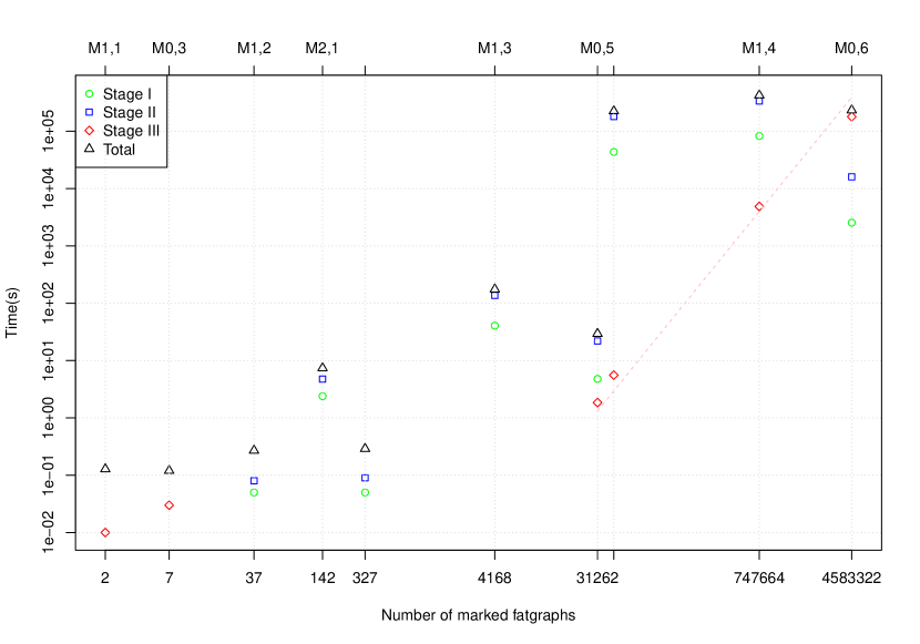
Figure 11. Scatter plot of the data in Table 4▷ Both axes use log⸧scale▷ Note how Stage III ↼computation of the boundary operators rank↽ becomes the dominant task as the number of marked fatgraphs increases▷

The scatter plot in Figure 11 shows that the time spent in computation of the $\mathitbf{D}^{(m)}$ matrix ranks done in Stage III can become the dominant contribution to the total running time as the number of fatgraphs increases▷ This highlights a limitation of the program. the large number of fatgraphs in the Kontsevich complex might turn out to be a challenge for todayφs sparse linear algebra software▷

However⸦ the set of fatgraphs for a given $(g,n)$ pair has to be generated prior to computing the matrices $\mathitbf{D}^{(m)}$. a very large set of graphs can exhaust the computerφs memory long before computation time becomes a blocking issue▷

7▷2 Application to other fatgraph complexes

In ♭godin:homology♯⸦ V▷ Godin defined a ℓℓbordered fatgraph complexφφ⸦ which computes the integral homology of the moduli spaces of Riemann surfaces with boundaries▷ Godinφs fatgraphs extend the abstract fatgraph by requiring that a leaf ↼i▷e▷⸦ a univalent vertex↽⸦ and only one⸦ is present in each boundary cycle▷ The bordered fatgraph complex is then constructed exactly as the fatgraph complex presented here⸦ with the proviso that an edge ending in a univalent vertex is never contracted. hence⸦ the differential $D$ is given by the sum of contraction of non⸧loop non⸧leaf edges▷

The algorithms of this paper can easily be adapted to compute the homology of Godinφs bordered fatgraph complex. after generating the family of marked fatgraphs of a given $(g,n)$ pair⸦ we decorate each marked fatgraph with leaves, compute the matrix form of the differential $D$ and then reduce it to Smith normal form to reckon the integral homology modules of the moduli space of bordered surfaces▷

There is no need for checking duplicates in the set of bordered fatgraphs so generated⸦ therefore the decoration step can be implemented efficiently▷ A shortcut can also be taken in computing the matrix $D$. since leaf edges are never contracted⸦ the differential on bordered fatgraphs can be deduced easily from the differential on marked fatgraphs▷ However⸦ the number of bordered fatgraphs is much larger than the number of marked fatgraphs,this means that the final linear algebra computations require even more computational resources than they do for $\mathcal{M}_{g,n}$ computations▷

7▷3 Future development directions

There are a number of directions in which the current algorithms and code could be improved▷

As already noted⸦ the generation algorithms produce quite a number of duplicates⸦ that have to be removed using a quadratic⸧complexity procedure▷ A variant of the ℓℓisomorph⸧free generationφφ algorithm of McKay ♭mckay:isomorph-free♯ could replace the naive εMgnTrivalentGraphsε code, the question of which algorithm would be faster has probably to be sorted out empirically⸦ the critical performance factor being the number of times the ℓℓisomorphismφφ test is invoked▷

Another approach would be to turn the generation procedure ℓℓupside downφφ. instead of starting with trivalent graphs and contracting edges⸦ one could start with $(g,n)$⸧fatgraphs with one vertex and expand those until the whole set of fatgraphs is generated▷ This would have the advantage that the chromatic fatgraph polynomial of Bollobás and Riordan ♭7♯ is available as an invariant to speed up the isomorphism procedure▷ On the other hand⸦ the number of fatgraphs generated this way seems consistently larger than the number of fatgraphs generated with the procedure adopted here ↼see Section A.2↽▷

So far⸦ the major obstacle to applying the algorithms of this paper to a wider range of moduli spaces has been the large number of fatgraphs involved. it affects both the total run time and memory consumption of the code▷ Most algorithms described here lend themselves naturally to parallelization⸦ so it would be possible to rewrite the program to exploit several processors and distributed memory⸦ which could solve both issues▷ However⸦ the number of generated fatgraphs grows super⸧exponentially in the asymptotic limit ♭3⸦ 4♯⸦ so any implementation of the algorithms outlined here will soon hit the limit of any present⸧day computing device▷ The question remains open⸦ whether more significant result could be obtained before hitting the limits of todayφs computers▷

Appendix A Comparison of fatgraph generation methods

This section compares three different approaches to generating trivalent fatgraphs. namely⸦ we compare the εMgnTrivalentGraphsε algorithm described in Section 5.1.3 with two alternatives▷ Table 5 presents a summary of results▷

None of the suggested algorithms is capable of directly producing an isomorph⸧free set of distinct fatgraphs, they all produce a larger set of fatgraphs that must be reduced by taking only one representative per isomorphism class of fatgraphs▷ Therefore⸦ Table 5 also reports the actual number of distinct fatgraphs for a given $g,n$ pair, not all counts are known. a cell is left empty when the corresponding count has not yet been computed▷ From the results gathered so far⸦ it is apparent that all algorithms overestimate the actual number of fatgraphs▷

$g$	$n$	$N$	$N_{1}^{+}$	$N_{2}^{+}$	$N_{3}$
0	3	2	$-$	15	$5\,760$
0	4	6	84	630	$1.072964\times 10^{13}$
0	5	26	936	15 015	$4.593811\times 10^{24}$
0	6	191	8 892	306 306	$6.326929\times 10^{37}$
0	7		114 600	5 819 814	$1.132261\times 10^{52}$
1	1	1	$-$	15	$5\,760$
1	2	5	114	630	$1.072964\times 10^{13}$
1	3	46	1 644	15 015	$4.593811\times 10^{24}$
1	4	669	24 156	306 306	$6.326929\times 10^{37}$
1	5		511 416	5 819 814	$1.132261\times 10^{52}$
2	1	9	6 336	15 015	$4.593811\times 10^{24}$
2	2	368	17 982	306 306	$6.326929\times 10^{37}$
2	3		606 144	5 819 814	$1.132261\times 10^{52}$
3	1		1 065 718 368 †	5 819 814	$1.132261\times 10^{52}$

Table 5. Number of ↼non⸧unique↽ trivalent fatgraphs generated according to different algorithms▷ The $N$ column reports the actual number of distinct fatgraphs for the given $g$⸦ $n$, empty cells mean the corresponding number has not been computed▷ The $N_{1}^{+}$ column lists upper bounds for the recursive generation algorithm MgnTrivalentGraphs ↼see Listing 7↽, values marked with the ℓℓ$\dagger$φφ symbol are estimated using earlier values of $N_{1}^{+}$ because the corresponding values of $N$ are not available▷ The $N_{2}^{+}$ values bound from above the number of fatgraphs generated by grafting binary trees into clovers▷ Finally⸦ $N_{3}$ is the count of fatgraphs generated by enumerating pairs of permutations ↼as per combinatorial definition of fatgraph↽▷

In what follows⸦ let $N(g,n):=\lvert\mathcal{R}_{g,n}\rvert$ be the number of distinct $(g,n)$⸧fatgraphs, also define.

$$\xi(g,n) :=2g+n,$$ (13)

$$m_{\text{max}}(g,n) :=6g+3n-6=3\xi-6,$$

$$m_{\text{min}}(g,n) :=2g+n-1=\xi-1.$$

It is trivial to check that $m_{\text{max}}$ and $m_{\text{min}}$ are the maximum and minimum number of edges that a $(g,n)$⸧fatgraph can have▷

A▷1 Generation by recursive edge addition

The algorithm MgnTrivalentGraphs described in Section 5.1.3 produces a $(g,n)$⸧fatgraph by adding an edge to fatgraphs with lower $(g,n)$, the procedure can then be applied recursively▷

Let $N_{1}(g,n)$ be the number of ↼non distinct↽ fatgraphs returned by εMgnTrivalentGraphs↼$g$⸦$n$↽ε▷ According to Section 5.1.3⸦ this can be written as.

$$N_{1}(g,n)=N_{1,A}(g,n)+N_{1,B}(g,n)+N_{1,C}(g,n),$$

where $N_{1,A}$⸦ $N_{1,B}$⸦ $N_{1,C}$ are the numbers of fatgraphs constructed in cases A↽⸦ B↽⸦ Cφ↽ of Algorithm 7▷

In case A↽⸦ we have 1 generated $(g,n)$⸧fatgraph per each pair formed by a $(g,n-1)$⸧fatgraph and one of its oriented edges⸦ modulo the action of the automorphism group $\operatorname{Aut}(G)$▷ However⸦ the number of orbits of this $\operatorname{Aut}(G)$⸧action is difficult to estimate▷ Since the generic fatgraph only has one automorphism⸦ an upper bound can instead be given by considering all pairs formed by a fatgraph and an oriented edge.

$$N_{1,A}(g,n)\leqslant N_{1,A}^{+}(g,n):=2\cdot m_{\text{max}}(g,n-1)\cdot N(g,n-1).$$

In case B↽⸦ the algorithm generates one $(g,n)$⸧fatgraph per each triplet formed by a $(g,n-1)$⸧fatgraph and two oriented edges⸦ not necessarily distinct ↼modulo the action of $\operatorname{Aut}G$↽, a similar remark about the upper bound applies.

$$N_{1,B}(g,n)\leqslant N_{1,B}^{+}(g,n):=(2\cdot m_{\text{max}}(g,n-1))^{2}\cdot N(g,n-1)$$

In case Cφ↽⸦ the computation is exactly the same⸦ except we apply the $q$ construction to fatgraphs belonging in $\mathcal{R}_{g-1,n+1}$.

$$N_{1,C}(g,n)\leqslant N_{1,C}^{+}(g,n):=4\cdot m_{\text{max}}(g-1,n+1)^{2}\cdot N(g-1,n+1).$$

Table 5 shows the upper bound given by

$$N_{1}^{+}(g,n):=N_{1,A}^{+}(g,n)+N_{1,B}^{+}(g,n)+N_{1,C}^{+}(g,n).$$

According to Table 5⸦ the εMgnTrivalentGraphsε algorithm outperforms the alternative procedures when $2g+n<7$⸦ and apparently generates a much larger set of fatgraphs when $2g+n>7$▷ However⸦ the values were obtained using $N_{1}^{+}(g,n)$ instead of $N(g,n)$ in recursive computations when the actual value of $N(g,n)$ is not known, therefore $N_{1}^{+}(g,n)$ might grossly overestimate the number of graphs considered by εMgnTrivalentGraphsε for $2g+n>6$▷ Further investigation is needed to ascertain whether this is due to the algorithm of Section A.2 being asymptotically faster⸦ or to the estimate for $N_{1}(g,n)$ being grossly imprecise when no data about the real number of trivalent fatgraphs in the recursion step is known▷ However⸦ the author conjectures that this estimate holds.

$$N_{1}(g,n)\leqslant O(\xi^{3})\cdot N(g,n)$$ (14)

A▷2 Generation by insertion of binary trees

A different approach is the following.

• Generate all distinct $(g,n)$⸧fatgraphs with 1 vertex, each such fatgraph has $m_{\text{min}}(g,n)$ edges⸦ hence the vertex has valence $2\cdot m_{\text{min}}(g,n)$▷

• Given any such fatgraph $G_{0}$⸦ build a trivalent $(g,n)$⸧fatgraph $G$ by replacing the vertex with a full binary tree on $2\cdot m_{\text{min}}(g,n)$ leaves▷

Call a fatgraph with only one vertex a clover▷ Let $N_{2}^{\prime}(g,n)$ be the number of distinct $(g,n)$⸧clovers, we can estimate it as follows▷

Lemma A▷1▷

The number of isomorphic clovers is equal to the number of orbits of the adjoint action of $(12\ldots 2m)$ over the set of self⸧conjugate permutations $\{\sigma_{1}\in\mathfrak{S}_{2m}:\sigma_{1}^{2}=\operatorname{id}\}$▷

Proof▷

Let $G_{0}=(L;\sigma_{0},\sigma_{1},\sigma_{2})$ be a $(g,n)$⸧fatgraph given in combinatorial form⸦ where $L=\{1,\ldots,2m\}$ and $\sigma_{i}\in\mathfrak{S}_{m}$▷ If $G_{0}$ is a clover⸦ then $\sigma_{0}$ is a permutation formed by just one cycle, without loss of generality we may assume $\sigma_{0}$ is the rotation $(12\ldots 2m)$▷ Let $G_{0}^{\prime}=(L;\sigma_{0}^{\prime},\sigma_{1}^{\prime},\sigma_{2})$ be another $(g,n)$⸧clover. by the same reasoning we have $\sigma_{0}^{\prime}=\sigma_{0}=(12\ldots m)$, if $f\colon G_{0}\to G_{0}^{\prime}$ is an isomorphism⸦ then $f$ commutes with $\sigma_{0}$ hence $f=\sigma_{0}^{j}$ for some $j|2m$▷ Therefore⸦ from $\sigma_{1}\circ f=f\circ\sigma_{1}^{\prime}$ we get $\sigma_{1}^{\prime}=\sigma_{0}^{-j}\circ\sigma_{1}\circ\sigma_{0}^{j}$▷ This proves the claim▷ ∎

Lemma A▷2▷

Let $L$ be a finite set of $l=p\cdot q$ elements▷ The number of permutations of $L$ which can be expressed as product of $q$ disjoint $p$⸧cycles is.

$$C(p,q)=\prod_{i=1}^{q}\prod_{j=1}^{p-1}(pi-j).$$ (15)

Proof▷

Without loss of generality we can assume $L=\{1,\ldots,pq\}$, let $\tau\in\mathfrak{S}_{pq}$ be a permutation composed of $q$ disjoint $p$⸧cycles▷ We can give a ℓℓcanonicalφφ form to $\tau$ if we order its cycles by stipulating that.

• a cycle $(a_{1}a_{2}\ldots a_{p})$ is always written such that $a_{1}=\min a_{i}$,

• $(a_{1}a_{2}\ldots a_{p})$ precedes $(b_{1}b_{2}\ldots b_{p})$ iff $\min a_{i}<\min b_{i}$▷

Now assume $\tau$ is written in this canonical form, then $a_{1}=1$ and we have $pq-1$ choices for the element $a_{2}=\tau(a_{1})$ following $a_{1}$ in the cycle⸦ $pq-2$ choice for the next element $a_{3}=\tau(a_{2})$⸦ and so on until the final element $a_{p}$ of the first cycle▷ Then starting element $a_{p+1}$ of the second cycle has to be the minimum element of $L\setminus\{a_{1},a_{2},\ldots,a_{p}\}$⸦ but we have $(p-1)q-1$ choices for $a_{p+2}=\tau(a_{p+1})$. an iterative argument proves the assertion▷ ∎

Lemma A▷3▷

The number of distinct self⸧conjugate permutations on a set of $l$ elements is given by $(l-1)!!:=(l-1)\cdot(l-3)\cdot\ldots\cdot 1$▷

Proof▷

A self⸧conjugate permutation $\tau$ on a set $L$ of $l=2m$ elements is the product of $m$ disjoint 2⸧cycles⸦ and the the result follows from Lemma A.2▷ ∎

Combining Lemma A.1 and A.3⸦ we immediately get the following estimate.

$$\frac{(2m-1)!!}{2m}\leqslant N_{2}^{\prime}(g,n)\leqslant(2m-1)!!,\qquad m=m_{\text{min}}(g,n),$$

where the upper bound comes from assuming that no two clovers can be transformed one into the other by a rotation⸦ and the lower bound comes from considering all clovers as part of the same equivalence class▷

In order to create a trivalent fatgraph from a clover⸦ we replace the vertex with a full binary tree with $l=2m$ leaves, equivalently⸦ we identify the leaves of the tree according to the same ℓℓgluing patternφφ that identifies half⸧edges in the clover▷

More precisely⸦ let $G_{0}=(L;\sigma_{0},\sigma_{1},\sigma_{2})$ be a clover⸦ with $L=\{1,\ldots,2m\}$ and $\sigma_{0}=(12\ldots 2m)$ as above▷ Let $L^{\prime}$ be set of leaves of a chosen binary tree $T$ and $f\colon L^{\prime}\to L$ a bijection▷ Now $\tau:=f^{-1}\circ\sigma_{1}\circ f$ is a fixed⸧point free involution on $L^{\prime}$. by identifying leaves of $T$ according to $\tau$⸦ we get a trivalent fatgraph $G$⸦ which we say is obtained by plugging $T$ into $G_{0}$ ↼by means of $f$↽▷

Given a permutation $\phi^{\prime}$ on $L^{\prime}$⸦ the map $f^{\prime}=f\circ\phi^{\prime}$ is a bijection and we have.

$$\tau^{\prime}={f^{\prime}}^{-1}\circ\sigma_{1}\circ f^{\prime}={\phi^{\prime}}^{-1}\circ(f^{-1}\circ\sigma_{1}\circ f)\circ\phi^{\prime}={\phi^{\prime}}^{-1}\circ\tau\circ{\phi^{\prime}},$$

which is an involution on $L^{\prime}$ conjugate to $\tau$▷ Conversely⸦ if $\sigma_{1}^{\prime}=\phi^{-1}\circ\sigma_{1}\circ\phi$ is conjugate to $\sigma_{1}$⸦ then $f^{\prime}=\phi\circ f\colon L^{\prime}\to L$ is again a bijection⸦ hence.

$${f}^{-1}\circ\sigma_{1}^{\prime}\circ f=(f^{-1}\circ\phi^{-1})\circ\sigma_{1}\circ(\phi\circ f)={f^{\prime}}^{-1}\circ\sigma_{1}\circ{f^{\prime}},$$

which is the involution defining the attachment map of $T$ to $G_{0}$ by means of $f^{\prime}$▷ Since any two involutions are conjugate⸦ we can fix the map $f$ once and for all binary trees with the same number of leaves⸦ and only let the involution $\sigma_{1}$ ↼i▷e▷⸦ the clover $G_{0}$↽ vary▷

Therefore $N_{2}(g,n)=N_{2}^{\prime}(g,n)\cdot Y({m_{\text{min}}(g,n))}$⸦ where $Y(l)$ is the count of full binary trees with $l$ leaves▷ The number $Y(l)$ is given by the $(l-1)$⸧th Catalan number.

$$Y(l)=\frac{(2l-2)!}{(l-1)!\cdot l!}.$$

Hence from (A.2) we get.

$$N_{2}^{-}(g,n)\leqslant N_{2}(g,n)\leqslant N_{2}^{+}(g,n),$$

where.

$$N_{2}^{-}(g,n):=\frac{1}{2m}\cdot\frac{(4m-2)!}{(2m-2)!!(2m)!},$$

$$N_{2}^{+}(g,n):=\frac{(4m-2)!}{(2m-2)!!(2m)!},$$ (16)

$$m:=m_{\text{min}}(g,n).$$

A▷3 Generation from permutations

As in the previous section⸦ represent a fatgraph $G$ in combinatorial form as $(L;\sigma_{0},\sigma_{1},\sigma_{2})$ where $L=\{1,\ldots,2m\}$▷ Here we count the number of trivalent fatgraphs that are generated by naively constructing a fatgraph from its combinatorial definition▷

If $G$ is trivalent⸦ then $\sigma_{0}$ is a product of disjoint 3⸧cycles, by Lemma A.2⸦ the number of such $\sigma_{0}$ is.

$$C(3,k)=(l-1)(l-2)\cdot(l-4)(l-5)\cdot\ldots\cdot 2\cdot 1,\qquad l=2m=3k$$ (17)

For each chosen $\sigma_{0}$⸦ each choice of a self⸧conjugate permutation $\sigma_{1}$ gives rise to a trivalent $(g,n)$⸧fatgraph, by Lemma A.3 there are exactly $(2m-1)!!$ such choices▷ Therefore⸦ we have.

$$\begin{split}N_{3}(g,n)=(2m-1)!!\cdot C(3,2m/3)=(2m-1)!!\cdot(2m-1)(2m-2)\cdot\\ \cdot(2m-4)(2m-5)\cdot\ldots\cdot 2\cdot 1,\end{split}$$ (18)

where $m=m_{\text{max}}(g,n)$▷

Appendix B Pseudo⸧code notation

Blocks of code are marked by indentation ↼rather than delimited by specific keywords↽▷

The ℓεdefεφ keyword is used to mark the beginning of a function definition▷

The notation ℓεfor $x$ in $S$εφ is used to loop over all the items $x$ in a set or sequence $S$, sometimes the notation ℓεfor x in $a,\ldots,b$εφ is used instead▷ The form ℓεfor $i,x$ in enumerate↼$S$↽εφ is used for keeping track of the iteration number when looping over the elements of $S$. as $x$ runs over the items in $S$⸦ $i$ orderly takes the values $0$⸦ $1$⸦ …⸦ up to $\lvert S\rvert-1$▷

B▷1 Basic types

Numbers and basic data structures ↼arrays⸦ lists⸦ sets, see below↽ are considered basic types⸦ together with the logical constants εTrueε and εFalseε⸦ and the special value εNoneε▷

B▷2 Objects

The word ℓℓobjectφφ is used to denote a kind of aggregate type. an object is a tuple ℓε↼$a_{1}$⸦ $a_{2}$⸦ $\ldots$⸦ $a_{N}$↽εφ⸦ where each of the slots ε$a_{i}$ε can be independently assigned a value, the values assigned to different $a_{i}$φs need not be of the same type▷ We write $X.a_{i}\leftarrow b$ to mean that the slot $a_{i}$ of object $X$ is assigned the value $b$▷ Unless otherwise noted⸦ object slots are mutable⸦ i▷e▷⸦ they can be assigned different values over the course of time▷

An objectsφ class is the tuple ℓε↼$a_{1}$⸦ $\ldots$⸦ $a_{N}$↽εφ of slots names that defines the object, the actual tuple of values is called an instance▷

B▷3 Arrays⸦ lists⸦ sets

A few types of basic data structures are used in the code. arrays⸦ lists and sets▷ They are distinguished only for clarity⸦ and we make no assumption that these are primitive. for instance⸦ each of these data structures could be implemented on top of the ℓℓlistφφ type defined here▷

An ℓℓarrayφφ is a fixed⸧size collection of elements of the same type, the number and type of elements stored in an array will be stated when the array is first created▷ Items in an array can be accessed by position. if $a$ is an array⸦ then its $k$⸧th element will be accessed as $a[k]$▷ Array elements can be mutated, we write $a[k]\leftarrow b$ to mean that object $b$ is stored into the $k$⸧th place of array $a$▷

A ℓℓlistφφ is a variable⸧size collection of objects▷ Two features distinguish lists from arrays. (1) lists can grow and shrink in size⸦ and (2) lists can store items of different types▷ If $l$ is a list with $n$ elements⸦ the notation ε$l$▷append↼$x$↽ε will be used to mean that $x$ should be added as $(n+1)$⸧th item in list $l$▷ Again⸦ the square bracket notation $l[k]$ is used to denote the value stored in the $k$⸧th place in $l$⸦ and $l[k]\leftarrow x$ means that the $k$⸧th slot of $l$ is mutated to the value $x$▷ The operator ℓℓ$+$φφ stands for concatenation when applied to lists▷

A ℓℓsetφφ is a mutable unordered collection of objects of the same type▷ The only relevant difference with sets in the mathematical sense of the word is that set variables are mutable. if $s$ is a set⸦ then ε$s$▷add↼$x$↽ε will be used to specify that $s$ should be mutated into the set $s\cup\{x\}$▷ No duplicates are admitted. if $x\in s$ and $x=y$⸦ then ε$s$▷add↼$y$↽ε does not alter $s$ in any way▷

The word ℓℓsequenceφφ will be used to denote any one of the above three▷ When $S$ is a sequence⸦ we define εsize↼$S$↽ε as the number of elements in $S$, if $S$ is a εlistε or εarrayε object⸦ valid indices into $S$ range from $0$ to εsize↼$S$↽⸧1ε▷

B▷3▷1 List comprehensions

A special syntax is used to form a list when its items can be gotten by applying a function or operation to the elements of another sequence▷

The notation ℓεL / ♭$f(x)$ for $x$ in $S$♯εφ makes $L$ into the list formed by evaluating function $f$ on each element in $S$⸦ analogously to the usual notation $\{f(x):x\in S\}$ for sets▷

As an extension⸦ the expression ℓεL / ♭$f(x)$ for $x$ in $S$ if $P(x)$♯εφ makes $L$ into the list of values of $f$ over the set $S^{\prime}$ of elements of $S$ for which the predicate $P(x)$ is true. $S^{\prime}=\{x:x\in S\wedge P(x)\}$▷

B▷4 Operators

The ℓℓεdivision. for integers $k$ and $n>0$⸦ the expression ε↼$k$ evaluates to the smallest non⸧negative residue of $k\mod n$▷

The ℓℓ$+$φφ operator normally denotes addition when applied to numbers⸦ and concatenation when applied to lists▷

Any other operator keeps it usual mathematical meaning▷

References

- [1] User ℓℓAlgoriφφ▷ Answer to MathOverflow question ℓℓBetti numbers of moduli spaces of smooth Riemann surfacesφφ▷ http.◁◁mathoverflow▷net◁questions◁38968◁betti⸧numbers⸧of⸧moduli⸧spaces⸧ϱof⸧smooth⸧riemann⸧surfaces◁39005ϑ39005⸦ September 2010▷
- [2] Enrico Arbarello and Maurizio Cornalba▷ Divisors in the moduli spaces of curves▷ In Lizhen Ji⸦ Scott Wolpert⸦ and Shing⸧Tung Yau⸦ editors⸦ Geometry of Riemann surfaces and their moduli spaces⸦ volume 14 of Surveys in Differential Geometry⸦ pages 1⸧⸧22▷ International Press⸦ Sommerville⸦ MA⸦ 2009▷ Pre⸧print available online at. http.◁◁arxiv▷org◁abs◁0810▷5373v2▷
- [3] Edward A▷ Bender and E▷ Rodney Canfield▷ The asymptotic number of maps on a surface▷ J▷ Combin▷ Theory⸦ Ser▷ A⸦ 43↼2↽.244⸧⸧257⸦ 1986▷
- [4] Edward A▷ Bender⸦ Zhicheng Gao⸦ and L▷ Bruce Richmond▷ The map asymptotics constant ▷ Electron▷ J▷ Combinatorics⸦ 15⸦ 2008▷
- [5] G▷ Bini⸦ G▷ Gaiffi⸦ and M▷ Polito▷ A formula for the Euler characteristic of ▷ Mathematische Zeitschrift⸦ 236↼3↽.491⸧⸧523⸦ 2001▷
- [6] Gilberto Bini and John Harer▷ Euler characteristics of moduli spaces of curves▷ Journal of the European Mathematical Society⸦ 13↼2↽.487⸧⸧512⸦ 2011▷
- [7] Béla Bollobás and Oliver Riordan▷ A polynomial of graphs on surfaces▷ Math▷ Ann▷⸦ 323↼1↽.81⸧⸧96⸦ 2002▷
- [8] Kenneth S▷ Brown▷ Cohomology of Groups▷ Number 87 in Graduate Texts in Mathematics▷ Springer⸧Verlag⸦ 1982▷
- [9] J▷⸧G▷ Dumas⸦ T▷ Gautier⸦ M▷ Giesbrecht⸦ P▷ Giorgi⸦ B▷ Hovinen⸦ E▷ Kaltofen⸦ B▷ D▷ Saunders⸦ W▷ J▷ Turner⸦ and G▷ Villard▷ LinBox. A Generic Library for Exact Linear Algebra▷ In A▷ Cohen⸦ X▷⸧S▷ Gao⸦ and N▷ Takayama⸦ editors⸦ Mathematical Software. ICMS 2002 ↼Proceedings of the first International Congress of Mathematical Software⸦ pages 40⸧⸧50▷ World Scientific⸦ 2002▷
- [10] Python Software Foundation▷ Python Programming Language ⸧⸧⸧ Official Website▷ http.◁◁www▷python▷org◁▷
- [11] Ezra Getzler▷ The moduli space of curves⸦ volume 129 of Progr▷ Math▷⸦ chapter Operads and moduli spaces of genus Riemann surfaces⸦ pages 199⸧⸧230▷ Birka}user⸦ Boston⸦ 1995▷ \newblock Pre⸧print available online at. \url{http.◁◁arxiv▷org◁abs◁alg⸧geom◁9411004}▷ \bibitem{getzler.1998} Ezra Getzler▷ \newblock Topological recursion relations in genus 2▷ \newblock In {\em {Integrable systems and algebraic geometry ↼Kobe◁Kyoto⸦ 1997↽}}⸦ pages 73⸧⸧106⸦ River Edge⸦ NJ⸦ 1998▷ World Scientific Publishing▷ \newblock Pre⸧print available at. \url{http.◁◁arXiv▷org◁abs◁math◁9801003}▷ \bibitem{getzler.1999} Ezra Getzler▷ \newblock {Resolving mixed Hodge modules on configuration spaces}▷ \newblock {\em Duke Math▷ J▷}⸦ 96↼1↽.175⸧⸧203⸦ 1999▷ \newblock Pre⸧print available online at. \url{http.◁◁arxiv▷org◁abs◁alg⸧geom◁9611003}▷ \bibitem{godin.homology} Véronique Godin▷ \newblock The unstable integral homology of the mapping class groups of a surface with boundary▷ \newblock {\em Math▷ Ann▷}⸦ 337↼1↽.15⸧⸧60⸦ 2007▷ \bibitem{gorinov.rational⸧cohomology⸧M1n} Alexei~G▷ Gorinov▷ \newblock {Rational cohomology of the moduli space of pointed genus curves}▷ \newblock Pre⸧print available online at. \url{http.◁◁www▷liv▷ac▷uk◁~gorinov◁}▷ \bibitem{harer⸧zagier,euler⸧characteristic} J▷~Harer and D▷~Zagier▷ \newblock The {E}uler characteristic of the moduli space of curves▷ \newblock {\em Invent▷ Math▷}⸦ 85↼3↽.457⸧⸧485⸦ 1986▷ \bibitem{harer,second⸧homology} John Harer▷ \newblock The second homology group of the mapping class group of an orientable surface▷ \newblock {\em Invent▷ Math▷}⸦ 72↼2↽.221⸧⸧239⸦ 1983▷ \bibitem{hulek⇁tommasi} Klaus Hulek and Orsola Tommasi▷ \newblock {Cohomology of the second Voronoi compactification of }⸦ 2011▷ \newblock Pre⸧print available at. \url{http.◁◁arxiv▷org◁abs◁1103▷6169}▷ \bibitem{kontsevich,1993} Maxim Kontsevich▷ \newblock Formal ↼non↽commutative symplectic geometry▷ \newblock In {\em The Gel\cprime fand Mathematical Seminars⸦ 1990⸧⸧1992}⸦ pages 173⸧⸧187▷ Birkh\εauser␣Boston⸦␣Boston⸦␣MA⸦␣1993▷␣␣␣␣␣␣␣␣␣␣␣␣␣␣\bibitem{kontsevich,feynman}␣␣␣␣Maxim␣Kontsevich▷␣␣␣␣␣␣␣\newblock␣Feynman␣diagrams␣and␣low⸧dimensional␣topology▷␣␣␣␣␣␣␣␣\newblock␣In␣{\em␣First␣European␣Congress␣of␣Mathematics⸦␣Vol▷\␣II␣↼Paris⸦␣␣␣␣␣␣␣␣1992↽}⸦␣pages␣97⸧⸧121▷␣Birkh{\εa}user⸦␣Basel⸦␣1994▷␣␣␣␣␣␣␣␣␣␣␣\bibitem{lando⸧zvonkin}␣Sergei~K▷␣Lando␣and␣Alexander~K▷␣Zvonkin▷␣␣␣␣␣␣␣\newblock␣{\em␣Graphs␣on␣surfaces␣and␣their␣applications}⸦␣volume␣141␣of␣{\em␣␣␣␣␣{E}ncyclopaedia␣of␣{M}athematical␣{S}ciences}▷␣␣␣␣␣␣␣␣\newblock␣Springer⸧Verlag⸦␣2008▷␣␣␣␣␣␣␣␣␣␣␣␣␣␣␣␣\bibitem{linbox.website}␣␣␣␣␣␣␣␣{\scshape␣LinBox}␣website▷␣␣␣␣␣␣\newblock␣\url{http.◁◁linalg▷org◁}▷␣␣␣␣␣␣␣␣␣␣␣␣␣\bibitem{mckay.isomorph⸧free}␣␣␣Brendan~D▷␣McKay▷␣␣␣␣␣␣␣\newblock␣{Isomorph⸧Free␣Exhaustive␣Generation}▷␣␣␣␣␣␣␣␣\newblock␣{\em␣Journal␣of␣Algorithms}⸦␣26↼2↽.306⸧⸧324⸦␣1998▷␣␣␣␣␣␣␣␣␣␣␣␣\bibitem{mondello.arXiv.0705▷1792v1}␣␣␣␣Gabriele␣Mondello▷␣␣␣␣␣␣\newblock␣Riemann␣surfaces⸦␣ribbon␣graphs␣and␣combinatorial␣classes▷␣␣␣␣\newblock␣In␣Athanase␣Papadopoulos⸦␣editor⸦␣{\em␣Handbook␣of␣{Teichm\εuller}␣␣␣␣␣␣theory}⸦␣volume~2⸦␣pages␣151⸧⸧216▷␣European␣Mathematical␣Society⸦␣2009▷␣␣␣␣␣␣␣␣␣␣␣␣␣␣␣\bibitem{mumford.1967}␣␣David␣Mumford▷␣␣\newblock␣{Abelian␣quotients␣of␣the␣Teichm{\εu}ller␣modular␣group}▷␣␣␣␣␣\newblock␣{\em␣J▷␣Analyse␣Math▷}⸦␣18.227⸧⸧244⸦␣1967▷␣␣␣␣␣␣␣␣␣␣␣␣\bibitem{penner⇁knudsen⇁wiuf⇁andersen.2009}␣␣␣␣␣Robert~Clark␣Penner⸦␣Michael␣Knudsen⸦␣Carsten␣Wiuf⸦␣and␣Joergen~Ellegaard␣␣␣␣␣␣␣␣␣Andersen▷␣␣␣␣␣\newblock␣{Fatgraph␣Models␣of␣Proteins}▷␣␣␣␣␣␣␣␣\newblock␣{\em␣Proteins}⸦␣277.32⸦␣2009▷␣␣␣␣␣␣␣␣␣\bibitem{tommasi.phd}␣␣␣Orsola␣Tommasi▷␣\newblock␣{\em␣{Geometry␣of␣Discriminants␣and␣Cohomology␣of␣Moduli␣Spaces}}▷␣␣␣␣\newblock␣PhD␣thesis⸦␣Radboud␣University␣Nijmegen⸦␣2005▷␣␣␣␣␣␣␣␣\newblock␣Available␣online␣at.␣␣␣␣\url{http.◁◁webdoc▷ubn▷ru▷nl◁mono◁t◁tommasi_o◁geomofdia▷pdf}▷␣␣␣␣␣␣␣␣␣\bibitem{totaro.1996}␣␣␣Burt␣Totaro▷␣␣␣␣\newblock␣{Configuration␣spaces␣of␣algebraic␣varieties}▷␣␣␣␣␣␣␣␣\newblock␣{\em␣Topology}⸦␣35↼4↽.1057⸧⸧1067⸦␣1996▷␣␣␣␣␣␣␣␣␣␣␣␣␣␣␣\bibitem{python.reference27}␣␣␣␣Guido␣van␣Rossum␣et~al▷␣\newblock␣{The␣Python␣2▷7␣Language␣Reference}▷␣␣\newblock␣Online␣document␣at.␣␣␣␣␣\url{http.◁◁docs▷python▷org◁2▷7◁reference◁index▷html}⸦␣February␣2012▷␣␣␣␣␣␣␣␣␣\end{thebibliography}ε