Slowing light with a coupled optomechanical crystal array

Abstract

We study the propagation of light in a resonator optical waveguide consisting of evanescently coupled optomechanical crystal array. In the strong driving limit, the Hamiltonian of system can be linearized and diagonalized. In this case we obtain the polaritons, which is formed by the interaction of photons and the collective excitation of mechanical resonators. By analyzing the dispersion relations of polaritons, we find that the band structure can be controlled by changing the related parameters. It has been suggested an engineerable band structure can be used to slow and stop light pulses.

I Introduction

Owing to its important application in many fields, such as, low-threshold lasing lasing , pulse delaydelay and optical memories memory01 ; memory02 ; memory03 , slow light attracts a great deal of practical interest. A number of schemes to delay and store light have been suggested, such as electromagnetically induced transparency (EIT) in the atomic ensembles EIT01 ; EIT02 , photonic crystal waveguide band edgesPC01 ; PC02 , solid-state multilayer semiconductor structuresolid , coupled resonator optical waveguide (CROW)CROW ; Fan01 ; Fan02 ; FPcavity , more complicated hybrid structure, e.g., coupled resonator optical waveguide doped with atomsSun01 ; Sun02 ; atom01 ; atom02 .

For a static photonic structure, for example a bare CROW, due to the limitation of delay-bandwidth product constraint, it is not suitable to stop light. To dynamically stop and release the light, a dynamically tunable system is required. Fan suggested that, if there are extra resonators side coupling to the optical cavity cells of the CROW, Fano interference can lead to a large change of bandwidth of the system when a small refractive index modulation is employedFan01 . The velocity of light can therefore be dynamically slowed down and even stopped. Unlike the case of EIT the light is coherently stored in a static way in the resonance cavity array. Based on this idea researchers have replaced optical resonators with atoms to couple to the resonators in the CROW and found that the light can be converted to collective excitations of atoms and then reversely converted and releasedSun01 ; atom02 .

Optomechanics opens a door to directly control the mechanical motion with light Review . Many applications of optomechanics have been proposed, for example, using cooled nanomechanical oscillators to test quantum mechanics QM , ultra-sensitive detection of force and dispalcementforce ; position , quantum optics and quantum information processing squeezing ; entanglement ; statepreparation .

Meanwhile, as a new quantum system, optomechanics is also used to stop light. EIT effect in cavity optomechanical system with a Bose-Einstein condensate (BEC) is suggested to slow the lightzhu . Research groups led respectively by PainterEITQM02 and KippenbergEITQM01 proposed slowing down light based on EIT in optomechanics. The photons are mapped onto the phonon modes instead of internal atomic degrees of freedom in the case of EIT in atomic ensembles. In fact, like the case of a CROW, an optical waveguide coupled to an optomechanical crystal array has been suggested to slow and stop light pulsePainter1 .

Motivated by the work mentioned above, this paper investigates the photon transmission in a homogeneous side coupled optomechanical crystal array, in which each optical resonator in the bare CROW couples to an extra mechanical resonator. The interaction between the mechanical mode and optical modes allows the photonic band structure of CROW to be modulated, allowing stopping and releasing light possible in our model. By adjusting the refractive index of the photonic crystal, the photons can be mapped onto the collective excitation of mechanical modes and then be stopped. Our scheme offers a patternable, compact and on-chip platform to slow and stop light.

The paper is organized as follows: In Sec. II we present our model of spatial periodic optomechanical crystal arrays, which consists of optomechanical crystal cells side-coupled each other. After linearizing the Hamiltonian, in Sec. III, we transform the system into momentum space and then use Bogoliubov transformation to diagonalise the Hamiltonian. Based on the dispersion relations of upper and lower branch polaritons obtained in previous section, take lower polariton for example, we investigate the band structure and demonstrate how slow down the velocity of polariton by compressing the bandwidth in Sec. IV. The final section concludes the paper.

II Derivation of model

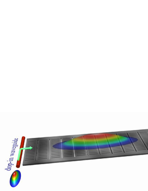
Figure 1: The schematic of 1-D periodic array of optomechanical crystals. Each optomechanical crystal cell is made up of photonic crystal and phononic crystal defect cavities coplanarPainter . The optomechanical crystal cells interact with each other by evanescent light field between them. The light pulse drops in and out by side-coupling wave guides.

We consider an 1-D periodic array of optomechanical crystals, which consists of $N$ evanescently coupled optomechanical crystals, shown in Figure 1. The single optomechanical crystal cell, co-localizing photonic and phononic resonances in a quasi one-dimensional optomechanical crystal, is proposed by the research group led by PainterPainter . The mechanical modes of the optomechanical crystal cell can be divided into common and differential modes of in-plane and out-plane motion of these nanobeams. For simplicity, we just consider the case that the gaps between the nanobeams are time-independent, i.e. the common mode case. Therefore the coupling between neighboring optical cavities is constant. To excite the system, a probe optical signal is dropped in the optomechanical array in a side-coupled configuration, and the output signal is dropped out in a similar manner. With this consideration, the Hamiltonian of the system in the reference frame rotating with probe laser frequency $\omega_{p}$ can be written as

$$H =H_{0}+H_{int}$$ (1a)

$$H_{0} =\sum_{i}\hbar\delta\hat{a}_{j}^{\dagger}\hat{a}_{j}+\sum_{j}\hbar\omega_{m}\hat{b}_{j}^{\dagger}\hat{b}_{j}$$ (1b)

$$H_{int} =\sum_{j}\hbar g\left(\hat{b}_{j}^{\dagger}+\hat{b}_{j}\right)\hat{a}_{j}^{\dagger}\hat{a}_{j}$$

$$-\sum_{j}\hbar G\left(\hat{a}_{j}^{\dagger}\hat{a}_{j+1}+\hat{a}_{j+1}^{\dagger}\hat{a}_{j}\right).$$ (1c)

here $$\hat{a}_{j}^{\dagger}\left(\hat{a}_{j}\right) \hat{b}_{j}^{\dagger}\left(\hat{b}_{j}\right) j \delta=\omega_{c}-\omega_{p} \omega_{m} g G$$ and are creation (annihilation) operators of optical cavity mode and mechanical mode in the -th optomechanical cell, respectively. is the detuning between cavity field and probe laser, is the mechanical resonator angular frequency, the constant is the coupling strength between cavity and mechanical resonator and denotes the nearest neighboring evanescently coupling of intercavity.

When the intracavity fields have a large amplitude, i.e. in the strong-driving limit, we can linearize the Hamiltonian by setting $\hat{f}=\left\langle f\right\rangle+\delta\hat{f}$ ($f=\hat{a}_{j},\hat{a}_{j}^{\dagger},\hat{b}_{j},\hat{b}_{j}^{\dagger}$), where $\left\langle f\right\rangle$ is the steady mean value and $\delta\hat{f}$ is the corresponding fluctuation around its steady value. With this ansatz, we then obtain the linearized Hamiltonian

$$H_{0} =\sum_{j}\hbar\omega_{m}\delta b_{j}^{\dagger}\delta b_{j}+\sum_{i}\hbar\tilde{\delta}\delta a_{j}^{\dagger}\delta a_{j}\allowbreak$$ (2)

$$H_{int} =\sum_{j}\hbar\tilde{g}\left(\allowbreak\delta a_{j}^{\dagger}\allowbreak\delta b_{j}+\delta a_{j}\delta b_{j}^{\dagger}\allowbreak\right)$$

$$-\sum_{j}\hbar G\left(\delta\hat{a}_{j}^{\dagger}\delta\hat{a}_{i+1}+\delta\hat{a}_{j+1}^{\dagger}\delta\hat{a}_{j}\right)$$ (3)

where the effective detuning is $\tilde{\delta}=\delta+g\left(\left\langle b\right\rangle+\left\langle b^{\ast}\right\rangle\right)/2$ and the effective coupling between light and mechanical vibration is $\tilde{g}=g\left\langle a\right\rangle$. In Eq. (3) we have omitted the counter-rotational wave term in the interaction between the cavity field and mechanical vibration.

III Dispersion of polariton

Let us study the Hamiltonian in $k$-representation. Taking into account the periodic properties of the system, we can make Fourier transformations

$$A_{k} =\frac{1}{\sqrt{N}}\sum_{j}\delta\hat{a}_{j}e^{ikjL}$$ (4a)

$$A_{k}^{\dagger} =\frac{1}{\sqrt{N}}\sum_{j}\delta\hat{a}_{j}^{\dagger}e^{-ikjL}$$ (4b)

$$B_{k} =\frac{1}{\sqrt{N}}\sum_{j}\delta\hat{b}_{j}e^{ikjL}$$ (4c)

$$B_{k}^{\dagger} =\frac{1}{\sqrt{N}}\sum_{j}\delta\hat{b}_{j}^{\dagger}e^{-ikjL}$$ (4d)

where $$A_{k}\left(A_{k}^{\dagger}\right) B_{k}\left(B_{k}^{\dagger}\right) k=2\pi n/LN n=0,1...N-1 L$$ are the normal mode operators of the coupled optical cavity, are the boson operators to describe the collective excitation (phonon) of mechanical resonators, with , and is the distance of inter-cavity. Inserting above transformation relation into Eqs. (1a), we arrive at the new Hamiltonian

$$H =\sum_{k}\hbar\omega_{m}B_{k}^{\dagger}B_{k}+\sum_{k}\hbar\omega_{ph}\left(k\right)A_{k}^{\dagger}A_{k}$$

$$+\sum_{k}\hbar\tilde{g}\allowbreak\left(\allowbreak A_{k}^{\dagger}\allowbreak B_{k}+B_{k}^{\dagger}\allowbreak A_{k}\allowbreak\right)$$ (5)

here $\omega_{ph}\left(k\right)=\tilde{\delta}-2G\cos\left(kL\right)$ is the original dispersion property of photon dependent on quasimomentum $k$ in the side-coupled photonic crystal cavity array. Hamiltonian (5) describes the interaction of the photonic and phononic modes.

To decouple the Hamiltonian (5), we introduce the Bogoliubov transformation

$$A_{k} =uC_{k}+vD_{k}$$ (6a)

$$A_{k}^{\dagger} =uC_{k}^{\dagger}+vD_{k}^{\dagger}$$ (6b)

$$B_{k} =vC_{k}-uD_{k}$$ (6c)

$$B_{k}^{\dagger} =vC_{k}^{\dagger}-uD_{k}^{\dagger}.$$ (6d)

and the inverse transformation is

$$C_{k} =uA_{k}+vB_{k}$$ (7a)

$$C_{k}^{\dagger} =uA_{k}^{\dagger}+vB_{k}^{\dagger}$$ (7b)

$$D_{k} =vA_{k}-uB_{k}$$ (7c)

$$D_{k}^{\dagger} =vA_{k}^{\dagger}-uB_{k}^{\dagger}$$ (7d)

Since operators $$C_{k} D_{k}$$ and must satisfy Bosonic commutation relations

$$\left[C_{k},C_{k}^{\dagger}\right] =1$$ (8)

$$\left[D_{k},D_{k}^{\dagger}\right] =1,$$ (9)

transformation coefficients $u$ and $v$ have the relation $u^{2}+v^{2}=1$. Substituting Eqs. (6) into Eq. (5), the Hamiltonian can be rewritten as

$$H =\left(\omega_{ph}\left(k\right)v^{2}+\omega_{m}u^{2}-2\tilde{g}uv\right)D_{k}D_{k}^{\dagger}\allowbreak$$

$$+\left(\omega_{ph}\left(k\right)u^{2}+\omega_{m}v^{2}+2\tilde{g}uv\right)C_{k}C_{k}^{\dagger}$$

$$+\left(\left(\omega_{ph}\left(k\right)-\omega_{m}\right)uv+\tilde{g}\left(v^{2}-u^{2}\right)\right)D_{k}C_{k}^{\dagger}$$

$$+\left(\left(\omega_{ph}\left(k\right)-\omega_{m}\right)uv+\tilde{g}\left(v^{2}-u^{2}\right)\right)D_{k}^{\dagger}C_{k}.$$ (10)

Obviously, if

$$\left(\omega_{ph}\left(k\right)\allowbreak-\omega_{m}\right)uv+\tilde{g}\left(v^{2}\allowbreak-u^{2}\right)=0$$ (11)

the Hamiltonian will have the diagonalized form

$$H=\sum_{k}\hbar\omega_{D}\left(k\right)D_{k}^{\dagger}D_{k}+\sum_{k}\hbar\omega_{C}\left(k\right)C_{k}^{\dagger}C_{k}.$$ (12)

From Eqs. (7) and (12) one can note that $C_{k}$ and $D_{k}$ operators represent two types of elementary excitations (phonon-photon polaritons) in coupled optomechanical array system, which is the result of the coherently mixing of photons and phonons through coupling in each optomechanics cell. The dispersion relations of lower and upper branches polaritons are determined by

$$\omega_{C}\left(k\right) =\frac{1}{2}\left(\omega_{m}+\omega_{ph}\left(k\right)-\sqrt{4\tilde{g}^{2}+\left(\omega_{ph}\left(k\right)-\omega_{m}\right)^{2}}\right)$$ (13)

$$\omega_{D}\left(k\right) =\frac{1}{2}\left(\omega_{m}+\omega_{ph}\left(k\right)+\sqrt{4\tilde{g}^{2}+\left(\omega_{ph}\left(k\right)-\omega_{m}\right)^{2}}\right).$$ (14)

It is found that the original single optical band structure is split into two bands owing to the interaction between photons and phonons.

IV Slowing light with tunable band structure

The bandwidths of lower and upper branches, respectively, are

$$\Delta_{WC} =\omega_{C}\left(\pi\right)-\omega_{C}\left(0\right)$$

$$=2G+\Delta$$ (15)

$$\Delta_{WD} =\omega_{D}\left(\pi\right)-\omega_{D}\left(0\right)$$

$$=2G-\Delta$$ (16)

where

$$\Delta=\sqrt{\tilde{g}^{2}+\left(\Delta_{OM}/2-G\right)^{2}}-\sqrt{\tilde{g}^{2}+\left(\Delta_{OM}/2+G\right)^{2}}$$ (17)

with the detuning $\Delta_{OM}=\tilde{\delta}-\omega_{m}$. Compared to the original optical band, the bandwidth of the lower branch polariton is enlarged and the upper one is compressed. Moreover, the most important thing is that both of these bandwidths of lower and upper bands can be modulated by changing parameters, such as $\tilde{g}$, $G$ and $\Delta_{OM}$. Figure 2 shows a typical picture of the bandwidth of lower branch polariton dependent on $\Delta_{OM}$, from which one can note that the bandwidth decreases with increasing $\Delta_{OM}$. In more detail, when $\Delta_{OM}/2\ll-\tilde{g}$, the bandwidth of lower band $\Delta_{WC}\simeq 4G$, corresponding to the maximum bandwidth; when $\Delta_{OM}/2\gg\tilde{g}$, the bandwidth is approximately equal to zero.

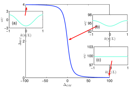
Figure 2: The bandwidth of lower branch polariton as a function of $\Delta_{0}$. The insets are the corresponding band structures of polariton when detuning (a)$\Delta_{0}=-100$; (b) $\Delta_{0}=0$ and (c) $\Delta_{0}=100$. $G=1$, $g=5$, $\omega_{m}=100$. Here $\Delta_{OM}$ is in units of $G$.

On the other hand, it is known that the group velocity of polaritons in a lattice is related with dispersion

$$v_{C,D} = \frac{\partial\omega_{C,D}\left(k\right)}{\partial k}$$ (18)

$$= -GL\sin\left(kL\right)\left(1\pm\frac{\Delta_{OM}-2G\cos\left(kL\right)}{\sqrt{4\tilde{g}^{2}+\left(\Delta_{OM}-2G\cos\left(kL\right)\right)^{2}}}\right).$$

which is also dependent on parameters $\tilde{g}$, $G$ and $\Delta_{OM}$ and therefore can be tuned. Such a tunable band structure leads to a tunable group velocity. Figure 3 shows the lower branch polariton with a momentum $kL=\pi/2$. We observe its group velocity decreases rapidly from its maximum value $G$ and vanishes as $\Delta_{OM}$ increases. In fact, such tunable band structure can play an important role in optical communication and quantum memory, for example, Fan suggested using a tunable CROW to slow and stop light pulseslowinglight .

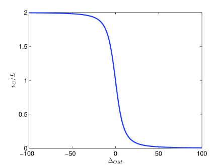
Figure 3: Velocity of lower branch polariton. Other parameters are the same as in Fig. 2.

Here we briefly demonstrate the process, taking the lower branch polariton as an example, to slow the light pulse in optomechanical crystal array. To begin with, the optical cavity is adjusted to be resonant with laser frequency, so the detuning is $\Delta_{OM}/2=-\omega_{m}/2\ll-\tilde{g}$. At this point, the bandwidth of lower branch is largest and can accommodate the entire light pulse, and the lower branch polariton is made up of photons, shown in figure 4. After the pulse enters completely into the optomechanical array, we then compress the bandwidth of lower branch polariton adiabatically by tuning the resonance frequency of the optical cavity until $\Delta_{OM}/2=\omega_{m}/2\gg\tilde{g}$. Further compressing the bandwidth, more and more photons are converted to mechanical modes in the lower branch, meanwhile, the velocity of polaritons slows down and approaches to zero.

From the point of conversion between photons and mechanical collective excitations, one can also understand the mechanism of stoping light. Because the total excitations number $N_{k}=B_{k}^{\dagger}B_{k}+A_{k}^{\dagger}A_{k}$ commutes with Hamiltonian $H$, when adjusting some parameters, such as $\Delta_{OM}$, the total excitations number is conserved, while the numbers of photons and mechanical collective excitations $A_{k}^{\dagger}A_{k}$ and $B_{k}^{\dagger}B_{k}$ are not conserved due to not commuting with the Hamiltonian. Hence the photons and mechanical collective excitations are mutually convertible, which results in mapping the light onto the mechanical vibration and vice versa. Figure 4 illustrates that the conversion between the photons and mechanical collective excitations. The number of mechanical collective excitation increases, from zero to unity, while the number of photons decrease from unity to zero, with increasing the detuning $\Delta_{OM}$.

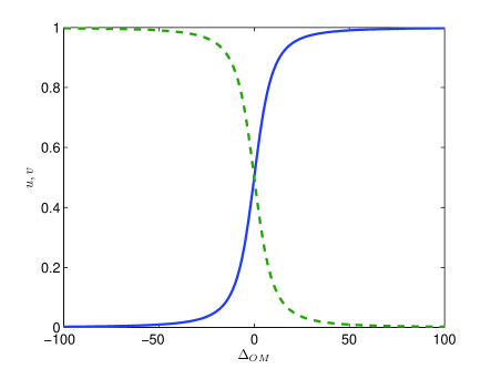
Figure 4: Transformation coefficients in the lower branch polariton versus detuning. The amplitude of $u$ and $v$ represent the ratio of photons and phonons in the lower branch polariton. Solid and dashed lines represents $v$ and $u$ respectively. Other parameters are the same as in Fig. 2.

We keep in mind that the rate of tuning cavity frequency should be less than the band gap between upper and lower branches, which is given by

$$\Delta_{WCD}\left(k\right)=\omega_{D}\left(k\right)-\omega_{C}\left(k\right)$$ (19)

This limitation avoids the polaritons in lower branch jumping up to the upper branch. Figure 5 shows that the band gap first linearly decreases and then linearly rises with increasing the detuning $\Delta_{OM}$. The minimum value of band gap is about $2G$ when the detuning of optical cavity is resonant with mechanical resonator.

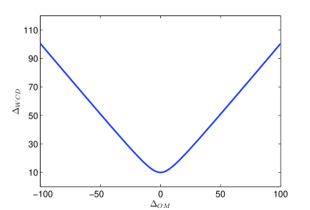
Figure 5: Band gap between upper and lower branches versus detuning. There is a minimum value when $\Delta_{OM}=0$. Other parameters are the same as in Fig. 2.

To practically stop light in the coupled optomechanics array, we tune the detuning between optical cavity field and probe laser by adjusting the refractive index of material,e.g. Si, which makes up of the optomechanical crystal. In our scheme, the amplitude of detuning modulation is the same order of magnitude of the mechanical resonance frequency, so the refractive index shift should be

$$\frac{\delta n}{n}\approx\frac{\delta\omega}{\omega_{0}}\sim 10^{-5}$$ (20)

which is feasible in practical optoelectronic devicesmodulation . Here we have taken the typical parameters $\omega_{c}/2\pi=200$ THz, $\omega_{m}/2\pi=10$ GHzPainter .

V Conclusion

We have studied the model of light transmission in a spatial periodic optomechanical crystal array. The optical cavities of the array evanescently couple to each other one by one to form a CROW. In the strong driving limit, we linearized the system and obtained the dispersion relations of lower and upper branch polaritons with Bogoliubov transformation in the momentum space. Our results show that the modulation of detuning between optical cavity and laser light can vary the bandwidths of polaritons, which has been demonstrated to be able to stop and release a light pulse.

VI Acknowledgments

We thank Andrew Bolt for polishing English.

References

- (1) K. Sakoda, Opt. Express 4, 167-176 (1999).
- (2) Yu. A. Vlasov, M. O’Boyle, H. F. Hamann and S. J. McNab, Nature 438, 65-69 (2005).
- (3) J. Scheuer, G. Paloczi, J. Poon, and A. Yariv, Opt. and Phot. News 16, 36 (2005).
- (4) N. Sangouard, C. Simon, H. de Riedmatten and N. Gisin, Rev. Mod. Phys. 83, 33–80 (2011)
- (5) K.F. Reim1, P. Michelberger, K.C. Lee, J. Nunn, N.K. Langford, and I.A. Walmsley, Phys. Rev. Lett. 107, 053603 (2011)
- (6) M. Fleischhauer and M. D. Lukin, Phys. Rev. Lett. 84, 5094–5097 (2000).
- (7) M. Fleischhauer, A. Imamoglu, J. Marangos, Rev. Mod. Phys. 77, 633–673 (2005).
- (8) Toshihiko Baba, Nature Photonics 2, 465 - 473 (2008).
- (9) Y.A. Vlasov, M. O’Boyle, H.F. Hamann, and S.J. McNab, Nature 438, 65-69 (2005).
- (10) A.V. Turukhin, V.S. Sudarshanam, M.S. Shahriar, J.A. Musser, B.S. Ham, and P.R. Hemmer, Phys. Rev. Lett. 88, 023602 (2001).
- (11) Qianfan Xu, Po Dong & Michal Lipson, Nature Physics 3, 406-410 (2007).
- (12) M.Y. and S. H. Fan, Phys. Rev. A 71, 013803 (2005).
- (13) Q. Xu, S. Sandhu, M.L. Povinelli, J. Shakya, S. Fan, and M. Lipson, Phys. Rev. Lett. 96, 123901(2006).
- (14) J.K.S. Poon, P. Chak, J.M. Choi, A. Yariv, JOSA B, 24, 2763-2769 (2007).
- (15) F. M. Hu, L. Zhou, T. Shi and C. P. Sun, Phys. Rev. A 76, 013819 (2007);
- (16) L. Zhou, J. Lu and C.P. Sun, Phys. Rev. A 76, 012313 (2007).
- (17) I O Barinov, A P Alodzhants and Sergei M Arakelyan, Quantum Electron. 39, 685 (2009).
- (18) A. P. Alodjants, I. O. Barinov and S. M. Arakelian, J. Phys. B: At. Mol. Opt. Phys. 43 095502 (2010).
- (19) F. Marquardt and S.M. Girvin, Physics 2 40 (2009).
- (20) W. Marshall, C. Simon,B. Penrose, D. Bouwmeester, Phys. Rev. Lett. 91, 130401 (2003).
- (21) J.D. Teufel, T. Donner, M.A. Castellanos-Beltran, J.W. Harlow, K.W. Lehnert, Nat. Nano., 4, 820–823, (2009).
- (22) A. Schliesser, O. Arcizet, R. Riviere, G. Anetsberger, T.J. Kippenberg, Nat. Phys., 5, 509–514 (2009).
- (23) C. Fabre, M. Pinard, S. Bourzeix, A. Heidmann, E. Giacobino, and S. Reynaud, Phys. Rev. A 49, 1337 (1994).
- (24) D. Vitali, S. Gigan, A. Ferreira, H. R. Bohm, P. Tombesi, A. Guerreiro, V. Vedral, A. Zeilinger, and M. Aspelmeyer, Phys. Rev. Lett. 98, 030405 (2007).
- (25) S. Bose, K. Jacobs, and P. L. Knight, Phys. Rev. A 56, 4175 (1997); W. Marshall, C. Simon, R. Penrose, and D. Bouwmeester, Phys. Rev. Lett. 91, 130401 (2003).
- (26) Chen Bin; Jiang Cheng; Zhu Ka-Di, Phys. Rev. A 83, 055803 (2011).
- (27) A. H. Safavi-Naeini, T. P. Mayer Alegre, J. Chan1, et.al., Nature 472, 69–73 (2011)
- (28) S. Weis1, R. Riviere, S. Deleglise, , et.al., Science, 330, 1520-1523 (2010).
- (29) D.E. Chang, A. H. Safavi-Naeini, M. Hafezi and O. Painter, New J. Phys. 13, 023003 (2011).
- (30) M. Eichenfield J. Chan, R.M. Camacho, et.al., Nature 459, 550 (2009).
- (31) M.Y. and S. H. Fan, Phys. Rev. Lett 92, 083901 (2004).
- (32) S.L. Chuang, Physics of optoelectronic Devices (Interscience, New York, 1995).