A mathematical treatment of bank monitoring incentives

Résumé

In this paper, we take up the analysis of a principal/agent model with moral hazard introduced in pages , with optimal contracting between competitive investors and an impatient bank monitoring a pool of long-term loans subject to Markovian contagion. We provide here a comprehensive mathematical formulation of the model and show using martingale arguments in the spirit of Sannikov san how the maximization problem with implicit constraints faced by investors can be reduced to a classical stochastic control problem. The approach has the advantage of avoiding the more general techniques based on forward-backward stochastic differential equations described in cviz and leads to a simple recursive system of Hamilton-Jacobi-Bellman equations. We provide a solution to our problem by a verification argument and give an explicit description of both the value function and the optimal contract. Finally, we study the limit case where the bank is no longer impatient.

JEL classification: G21 - G28 - G32

1 Introduction

Following the seminal contributions of DeMarzo and Fishman demarzo4 , demarzo5 and Sannikov san , there has been a renewed interest in the mathematical treatment of continuous-time moral hazard models and their applications. In a typical moral hazard situation, a principal (who takes the initiative of the contract) is imperfectly informed about the action of an agent (who accepts or rejects the contract). The goal is to design a contract that maximizes the utility of the principal while that of the agent is held to a given level.

In its whole generality, the mathematical treatment of the problem can be cast as follows. Agency problems stemming from the agent’s hidden action $a$ limit the utility this agent can get from contracting with the principal. The optimal contract specifies how these limitations should be strenghtened or slackened over time as a result of the agent’s ongoing performance. We first have to solve the agent’s problem for a given contract $c$

$$V_{A}(c):=\underset{a}{\sup}\ \mathbb{E}\left[U_{A}(c,a)\right],$$

where $U_{A}$ is the utility function of the agent. If we assume for simplicity that there exists a unique optimal action $a(c)$ for any $c$, a point on the set of constrained Pareto optima can be found by solving the Principal’s stochastic control problem

$$V_{P}:=\underset{c}{\sup}\left\{\mathbb{E}\left[U_{P}(c,a(c))\right]+\lambda\mathbb{E}\left[U_{A}(c,a(c))\right]\right\},$$

where $U_{P}$ is the utility function of the principal and $\lambda$ is the Lagrange multiplier associated to some reservation utility of the agent.

Because of the almost limitless choices for $c$, it is generally assumed that the agent does not have complete control over the outcomes but instead continuously affects their distribution by choosing specific actions. This actually means that the agent affects the probability measure $\mathbb{P}^{a}$ under which the above expectations are taken. This setting, which will be described more rigorously in the following section, corresponds to a weak formulation of the stochastic control problem.

As shown in cviz , a general theory can be used to solve these problems, by means of forward-backward stochastic differential equations. We show here how recursive, martingale representation-based techniques proposed by Sannikov san can be brought to bear on the issue to yield explicit solutions that are easy to derive. The paper is a companion to Pagès pages , who contributes to the optimal design of securitization in the presence of banks’ impaired incentives to monitor. It provides a coherent mathematical framework for this problem and lays down the rigorous foundations for the formal derivations sketched in pages .

Our point is to show that the martingale approach to contracting can be extended to a Markovian setting, which makes it possible to relax the assumption of conditional independence between default times. There are now papers on jump processes as opposed to diffusions, but to the best of our knowledge they only deal with Poisson risk. In the theory of repeated games with imperfect monitoring, Abreu et al. abreu use Poisson signals to vary the frequency with which actions are taken, and show that the optimal provision of incentives is markedly different should the signals be interpreted as “good” or “bad” news. Sannikov and Skrzypacz san3 find in a continuous-time setting, with both Brownian information and Poisson jumps associated with bad news, that deviations from cooperative behavior can only be punished when the discontinuous information is revealed. This echoes former results in san2 , according to which collusion is impossible under imperfect monitoring with Brownian information, as the risk of triggering a punishment when no deviation occurs is large. A model close to ours is Biais et al. biais2 , who deal with large and unfrequent Poisson losses suffered by a firm that invests in a stationary environment. They show that an optimal way to restore incentives when performance is poor is to downsize the project at any time there is a loss.

Intensity-based models have been widely used in risk management. Here we focus on a contagion model with interacting default intensities. Frey and Backhaus frey show how such models can be conveniently embedded into a Markovian framework. Under this approach, a Markov chain is defined on the set of all default configurations which, when names are exchangeable, simply boil down to the portfolio default count, and default intensities are explicit functions of time and the portfolio default state, as exemplified by davis , jar and yu in the credit field. Markov chains have recently been shown to simplify the task of pricing and hedging credit risk, as in Kraft and Steffensen kraft or Laurent et al. laurent . They are also useful in our context, as they provide an alternative way of tackling problems of optimal contracting, even though the conditions under which explicit solutions can be derived are not warranted a priori.

The rest of the paper is organized as follows. In section 2, we recall the model laid out in pages , describe the contracts and give our main assumptions. In Section 3, we formally derive a candidate optimal contract by solving the HJB equation associated to the control problem. We then use a standard verification argument to show that the candidate solution is indeed the optimal contract and provide a numerical example. The paper concludes with a short section devoted to a simple special case.

2 The model

2.1 Notations and preliminaries

We consider a model with universal risk neutrality in which time is continuous and indexed by $t\in\left[0,\infty\right)$. Without loss of generality, the risk-free interest rate is taken to be $0$. A bank has a claim to a pool of $I$ unit loans indexed by $i=1$, $\dots$,$\leavevmode\nobreak\ I$ which are ex ante identical. Each loan is a defaultable perpetuity yielding cash flow $\mu$ per unit time until it defaults. Once a loan defaults it gives no further payments. The infinite maturity and no recovery assumptions are made for tractability.

Denote by

$$N_{t}=\sum_{i=1}^{I}1_{\left\{\tau^{i}\leq t\right\}},$$

the sum of individual loan default indicators, where $\tau^{i}$ is the default time of loan $i$. The current size of the pool is $I-N_{t}$. Since all loans are a priori identical, they can be reindexed in any order after defaults. The action of the bank consists in deciding at each time $t$ whether it monitors any of the outstanding loans. These actions are summarized by the functions $e_{t}^{i}$ such that for $1\leq i\leq I-N_{t},\text{ }e_{t}^{i}=1$, if loan $i$ is monitored at time $t$, and $e_{t}^{i}=0$ otherwise.

Non-monitoring renders a private benefit $B>0$ per loan and per unit time to the bank. The opportunity cost of monitoring is thus proportional to the number of monitored loans.

The rate at which loan $i$ defaults is controlled by the hazard rate $\alpha_{t}^{i}$ specifying its instantaneous probability of default conditional on history up to time $t$. Individual hazard rates are assumed to depend both on the monitoring choice of the bank and on the size of the pool. Specifically, we choose to model the hazard rate of a non-defaulted loan $i$ at time $t$ as

$$\alpha_{t}^{i}=\alpha_{I-N_{t}}\left(1+(1-e_{t}^{i})\varepsilon\right),$$ (1)

where the parameters $\left\{\alpha_{j}\right\}_{1\leq j\leq I}$ represent individual “baseline” risk under monitoring when the number of loans is $j$ and $\varepsilon$ is the proportional impact of shirking on default risk.

We define the shirking process $k$ by

$$k_{t}=\sum_{i=1}^{I-N_{t}}\left(1-e_{t}^{i}\right),$$

which represents the number of loans that the bank fails to monitor at time $t$. Then, according to (1), aggregate default intensity is given by

$$\lambda_{t}^{k}=\alpha_{I-N_{t}}\left(I-N_{t}+\varepsilon k_{t}\right).$$ (2)

The bank can fund the pool internally at a cost $r\geq 0$. It can also raise funds from a competitive investor who values income streams at the prevailing riskless interest rate of zero. We assume that both the bank and investors observe the history of defaults and liquidations.

2.2 Description of the contracts

Contracts are offered on a take-it-or-leave-it basis by investors to the bank and agreed upon at time $0$. They determine how cash flows are shared and how loans are liquidated, conditionally on past defaults and liquidations. Without loss of generality, they specify that an investor receives cash flows from the pool and makes transfers to the bank. We denote by $D=\left\{D_{t}\right\}_{t\geq 0}$ the càdlàg, positive and increasing process describing cumulative transfers from the investors to the bank, such that

$$\mathbb{E}^{\mathbb{P}}\left[D_{\tau}\right]<+\infty,$$ (3)

where $\tau$ is the liquidation time of the pool and where we assume that $D_{0}=0$.

Remark 1

For certain interpretations, it will be useful to let $D$ have a jump at time 0 (cf. Remark 4).

Let then $H_{t}:=1_{\left\{t\geq\tau\right\}}$ be the liquidation indicator of the whole pool. The contract specifies the probability $\theta_{t}$ with which the pool is maintained given default ($dN_{t}=1$), so that at each point in time

$$dH_{t}=\left\{\begin{tabular}[]{ll}$0$&with probability $\theta_{t},$\\ $dN_{t}$&with probability $1-\theta_{t}.$\end{tabular}\ \right.$$

With our notations,the hazard rates associated with the default and liquidation processes $N_{t}$ and $H_{t}$ are $\lambda_{t}^{k}$ and $\left(1-\theta_{t}\right)\lambda_{t}^{k}$, respectively.

The contract also specifies when liquidation occurs. We assume that liquidations can only take the form of the stochastic liquidation of all loans following immediately default. The above properties translate into

$$\mathbb{P}\left(\tau\in\left\{\tau^{1},...,\tau^{I}\right\}\right)=1,\text{ and }\mathbb{P}(\tau=\tau^{i}|\mathcal{F}_{\tau^{i}},\tau>\tau^{i-1})=1-\theta_{\tau^{i}}.$$

We summarize the above details of the contracts, which are completely specified by the choice of $(D,\theta)$. Each infinitesimal time interval $\left(t,t+dt\right)$ unfolds as follows:

• $I-N_{t}$ loans are performing at time $t$.

• The bank chooses to leave $k_{t}\leq I-N_{t}$ loans unmonitored and monitors the $I-N_{t}-k_{t}$ others, enjoying private benefits $k_{t}B\,dt$.

• The investor receives $\left(I-N_{t}\right)\mu\,dt$ from the cash flows generated by the pool and pays $dDt\geq 0$ as fees to the bank.

• With probability $\lambda_{t}^{k}\,dt$ defined by (2) there is a default ($dN_{t}=1$).

• Given default the pool is maintained ($dH_{t}=0$) with probability $\theta_{t}$ or liquidated ($dH_{t}=1$) with probability $1-\theta_{t}$.

2.3 Economic assumptions

In this section we make some assumptions arising from economic considerations (see pages for details). They are in force throughout the paper.

Assumption 2.1

$$\mu\geq\overline{\alpha}_{I}.$$ (4)

This condition ensures that monitored loans are profitable viewed as of time 0.

Assumption 2.2

We have for all $j\leq I$

$$\frac{r}{\overline{\alpha}_{j}}\leq\frac{\mu\varepsilon-B}{B}\frac{\varepsilon}{1+\varepsilon},$$

The condition is related to the efficiency of monitoring and ensures that the benefits for a non-monitoring bank are not so high that shirking is socially preferable.

Assumption 2.3

Individual default risk is non-decreasing with past default

$$\alpha_{j}\leq\alpha_{j-1},\qquad\text{for all }j\leq I.$$ (5)

The condition introduces the possibility of correlated defaults through a contagion effect, as individual loans’ intensity of default may increase with the arrival of new defaults.

The expected surplus that can be extracted from the pool of loans is

$$S=\mathbb{E}\left[\int_{0}^{\infty}\left(I-N_{t}\right)\mu\,dt\right]-I =\mathbb{E}\left[\sum_{j=1}^{I}\int_{0}^{\infty}j\mu 1_{\left\{I-N_{t}=j\right\}}\,dt\right]-I$$

$$=I\left(\mu/\overline{\alpha}_{I}-1\right),$$ (6)

which is positive under Assumption 2.1. Indeed, investors could commit $I$ to the pool, pay the bank $D_{0}=S$ at time 0, and instruct it to choose $k=0$ until the default of the last loan. They would break even from (6). We assume that the bank’s monitoring decision is not observable. This leads to a dynamic moral hazard problem, as the bank may choose $k_{t}>0$ down the road to reap the private benefits $k_{t}B$. The contract $\left(D,\theta\right)$ must use observations on defaults to give the bank incentives to monitor. We assume that both the bank and investors can fully commit to such a contract.

3 Optimal contracting

Before going on, let us now describe the stochastic basis on which we are working. We will always place ourselves on a probability space $(\Omega,\mathbb{F},\mathbb{P})$ on which $N$ is a Poisson process with intensity $\lambda_{t}^{0}$ (which is defined by (2)) and where $\mathbb{P}$ is the reference probability measure. We denote $(\mathcal{F}_{t}^{N})_{t\geq 0})$ the completed natural filtration of $N$ and by $(\mathcal{G}_{t})_{t\geq 0}$ the minimal filtration containing $(\mathcal{F}_{t}^{N})_{t\geq 0})$ and that makes the liquidation time of the pool $\tau$ a $\mathcal{G}$-stopping time. We note that this filtration satisfies the usual hypotheses, and therefore we will always consider super or submartingales in their càdlàg version.

3.1 Incentive compatibility and limited liability

As recalled in the introduction, in order to make the problem tractable, we assume that the monitoring choices of the bank affect the distribution of the size of the pool. To formalize this, recall that, by definition, the shirking process $k$ is $\mathcal{G}$-predictable and bounded. Then, by Girsanov Theorem, we can define a probability measure $\mathbb{P}^{k}$ equivalent to $\mathbb{P}$ such that

$$N_{t}-\int_{0}^{t}\lambda_{t}^{k}ds,$$

is a $\mathbb{P}^{k}$-martingale.

More precisely, we have from Brémaud bre (Chapter VI, Theorem T3) that on $\mathcal{G}_{t}$

$$\frac{d\mathbb{P}^{k}}{d\mathbb{P}}=Z_{t}^{k},$$

where $Z^{k}$ is the unique solution of the following SDE

$$Z_{t}^{k}=1+\int_{0}^{t}Z_{s^{-}}^{k}\left(\frac{\lambda_{s}^{k}}{\lambda_{s}^{0}}-1\right)\left(dN_{s}-\lambda_{s}^{0}ds\right),\text{ }0\leq t\leq T,\text{ }\mathbb{P}-a.s.$$

Then, given a contract $\left(D,\theta\right)$ and a shirking process $k$, the bank’s expected utility at $t=0$ is given by

$$u_{0}^{k}(D,\theta):=\mathbb{E}^{\mathbb{P}^{k}}\left[\int_{0}^{\tau}e^{-rt}(dD_{t}+Bk_{t}\,dt)\right],$$ (7)

while that of the investor is

$$v_{0}^{k}(D,\theta):=\mathbb{E}^{\mathbb{P}^{k}}\left[\int_{0}^{\tau}\left(I-N_{t}\right)\mu\,dt-dD_{t}\right].$$ (8)

Following Sannikov san , we give now the definition of an incentive-compatible shirking process.

Definition 1

A shirking decision $k$ is incentive-compatible with respect to the contract $\left(D,\theta\right)$ if it maximizes (7).

Then, the problem faced by the investors is to design a contract $\left(D,\theta\right)$ and an incentive-compatible advice on $k$ that maximize their expected discounted payoff, subject to a given reservation utility for the bank

$$v_{I}(u):= \underset{(D,\theta)}{\sup}\mathbb{E}^{\mathbb{P}^{k}}\left[\int_{0}^{\tau}\left(I-N_{t}\right)\mu dt-dD_{t}\right]$$ (9)

subject to $$\mathbb{E}^{\mathbb{P}^{k}}\left[\int_{0}^{\tau}e^{-rt}(dD_{t}+Bk_{t}\,dt)\right]\geq u$$

$$k\text{ incentive-compatible with respect to }\left(D,\theta\right).$$

This allows us to define a first set of admissible contracts for a given monitoring advice $k$

$$\mathcal{A}^{k}(x):=\{ (D,\theta),\text{ }\theta\in[0,1]\text{ is a predictable process},\ D\text{ is positive, c\`{a}dl\`{a}g,}$$

non-decreasing and satisfies (3), $$k$$ is incentive-compatible

$$\text{with respect to $\left(D,\theta\right)$ and $u_{0}^{k}(D,\theta)\geq x$}\}.$$ (10)

Notice that we will put more restrictions on this set at the end of the section.

Using martingale arguments, we now elicit an equivalent condition for the incentive compatibility of $k$. Consider the bank’s expected lifetime utility, conditional on $\mathcal{G}_{t}$

$$U_{t}^{k}(D,\theta):= \mathbb{E}^{\mathbb{P}^{k}}\left[\int_{0}^{\tau}e^{-rs}\left(dD_{s}+Bk_{s}ds\right)\Bigm{|}\mathcal{G}_{t}\right]$$

$$= \int_{0}^{t\wedge\tau}e^{-rs}\left(dD_{s}+Bk_{s}ds\right)+e^{-rt}u_{t}^{k}(D,\theta),$$

where $u_{t}^{k}$ is the dynamic version of the bank’s continuation utility defined as

$$u_{t}^{k}(D,\theta):=1_{\left\{t<\tau\right\}}\mathbb{E}^{\mathbb{P}^{k}}\left[\int_{t}^{\tau}e^{-r(s-t)}\left(dD_{s}+Bk_{s}ds\right)\Bigm{|}\mathcal{G}_{t}\right].$$ (12)

Since we are working with the completed natural filtration of a Poisson process, and since $U_{t}^{k}$ is a $\mathcal{G}_{t}$-martingale under $\mathbb{P}^{k}$ and in $L^{1}$ because of the integrability assumptions we made, the martingale representation theorem for point processes (see bre , Chapter III, Theorems $T9$ and $T17$, and Chapter VI, Theorems $T2$ and $T3$) implies that there are predictable processes $h^{1}$ and $h^{2}$ such that the bank’s continuation utility $u^{k}$ satisfies the following “promise-keeping” equation until liquidation occurs

$$du_{t}^{k}+\left(dD_{t}+Bk_{t}dt\right)=ru_{t}^{k}\,dt-h_{t}^{1}\left(dN_{t}-\lambda_{t}^{k}\,dt\right)-h_{t}^{2}\left(dH_{t}-(1-\theta_{t})\lambda_{t}^{k}\,dt\right),$$ (13)

where the dependence of $h^{1}$ and $h^{2}$ on $k$ has been suppressed for notational convenience. The introduction of these processes provides a practical way of characterizing contracts for which a given $k$ is incentive-compatible, as shown in the following proposition, inspired by Sannikov san . They have the interpretation of “penalties” weighing down the bank’s continuation utility, the first upon default ($dN_{t}=1$), and the second upon liquidation ($dH_{t}=1$).

Proposition 1

Given a contract $\left(D,\theta\right)$ and a shirking process $k$, the latter is incentive-compatible if and only if for all $t\in\left[0,\tau\right]$ and for all $i=1$, $\cdots$, $I-N_{t}$, the following holds almost-surely,

$$\left(\frac{B}{\varepsilon\alpha_{I-N_{t}}}-h_{t}^{1}-(1-\theta_{t})h_{t}^{2}\right)(k_{t}-i)\geq 0.$$ (14)

Proof. Consider an arbitrary strategy $\widehat{k}$ specifying the number of unmonitored loans at any point in time until liquidation. Let $u_{t}^{k}$ denote the continuation utility in (12) resulting from the decision to forgo monitoring $k$ loans at all times.

Define by

$$\widehat{U}_{t}=\int_{0}^{t\wedge\tau}e^{-rs}\left(dD_{s}+B\widehat{k}_{s}ds\right)+e^{-rt}u_{t}^{k}$$ (15)

the lifetime utility of the bank viewed as of time$\leavevmode\nobreak\ t$ if it follows the strategy $\widehat{k}$ before time $t$, and plans to switch to $k$ afterwards.

We have for all $t\in\left[0,\tau\right]$

$$d\widehat{U}_{t} =e^{-rt}\left(dD_{t}+B\widehat{k}_{t}dt\right)+e^{-rt}\left(du_{t}^{k}-ru_{t}^{k}\,dt\right)$$

$$=e^{-rt}B(\widehat{k}_{t}-k_{t})\,dt-e^{-rt}\left(h_{t}^{1}(dN_{t}-\lambda_{t}^{k}\,dt)+h_{t}^{2}(dH_{t}-(1-\theta_{t})\lambda_{t}^{k}\,dt)\right)$$

$$=e^{-rt}\left(B-\alpha_{I-N_{t}}\varepsilon(h_{t}^{1}+(1-\theta_{t})h_{t}^{2})\right)(\widehat{k}_{t}-k_{t})dt$$

$$\hskip 8.99994pt-e^{-rt}\left(h_{t}^{1}(dN_{t}-\lambda_{t}^{\widehat{k}}\,dt)+h_{t}^{2}(dH_{t}-(1-\theta_{t})\lambda_{t}^{\widehat{k}}\,dt)\right),$$

where we have used the promise-keeping equation (13) for  $u^{k}$. Therefore, the first term on the right-hand side

$$e^{-rt}\left(B-\alpha_{I-N_{t}}\varepsilon(h_{t}^{1}+(1-\theta_{t})h_{t}^{2})\right)(\widehat{k}_{t}-k_{t}),$$

is the drift of $\widehat{U}$ under $\mathbb{P}^{\widehat{k}}$. Note also that, by definition, $h^{1}$ and $h^{2}$ are integrable and therefore the martingale part of $\widehat{U}$ is a true $\mathbb{P}^{\widehat{k}}$-martingale.

$\mathrm{(i)}$ Now assume that (14) does not hold on a set of positive measure, and choose $\widehat{k}$ such that it maximizes the quantity

$$\left(B-\alpha_{I-N_{t}}\varepsilon(h_{t}^{1}+(1-\theta_{t})h_{t}^{2})\right)\widehat{k}_{t},$$

for all $t$. Then, the drift of $\widehat{U}$ under $\mathbb{P}^{\widehat{k}}$ is non-negative and strictly positive on a set of positive measure. Therefore $\widehat{U}$ is a $\mathbb{P}^{\widehat{k}}$-submartingale. This implies the existence of a time $t^{\ast}>0$ such that

$$\mathbb{E}^{\mathbb{P}^{\widehat{k}}}[\widehat{U}_{t^{\ast}}]>\widehat{U}_{0}=u_{0}^{k}.$$

Therefore, if the agent follows this strategy $\widehat{k}$ until the time $t^{\ast}$ and then switches to the strategy $k$, his utility is strictly greater than the utility obtained from following the strategy $k$ all the time. This contradicts the fact that the strategy $k$ is incentive-compatible.

$\mathrm{(ii)}$ With the same notations as above, assume that (14) holds for the strategy $k$. Then this means that $\widehat{U}$ is a $\mathbb{P}^{\widehat{k}}$-supermartingale, regardless of the choice of strategy $\widehat{k}$. Moreover, since $\widehat{U}$ is positive (because $D$ is non-decreasing), it has a last element (see Problem $3.16$ in karat for instance). Then, we have by the optional sampling Theorem

$$u_{0}^{k}=\widehat{U}_{0}\geq\mathbb{E}^{\mathbb{P}^{\widehat{k}}}\left[\widehat{U}_{\tau}\right]=u_{0}^{\widehat{k}},$$

where we used (15) and the fact that $u_{\tau}^{k}=0$ for the last inequality. This means that the strategy $k$ maximizes the expected utility of the agent and is therefore incentive-compatible. $\Box$

Under the assumption that monitoring is efficient, we now focus on contracts that actually deter the bank from shirking, i.e., contracts with respect to which $k=0$ is incentive-compatible. In that particular case, the above Proposition can be simplified as follows.

Corollary 1

Given a contract $\left(D,\theta\right)$, $k=0$ is incentive-compatible if and only if

$$h_{t}^{1}+(1-\theta_{t})h_{t}^{2}\geq\frac{B}{\varepsilon\alpha_{I-N_{t}}},\text{ }t\in[0,\tau],\text{ }\mathbb{P}-a.s.$$ (16)

Remark 2

Corollary 1 states that, given that the pool has $i$ loans outstanding, in order to induce the bank to monitor all loans, the continuation payoff must drop in expectation by at least the quantity

$$b_{i}:=\frac{B}{\varepsilon\alpha_{i}},$$

following default.

In order to specify further our admissible strategies, we have to put some restrictions on $h^{1}$ and $h^{2}$. First, we assume that the bank has limited liability. This means that the bank’s continuation utility is bounded from below by $b_{I-N_{t}}$ up to liquidation, since otherwise the incentive-compatible (16) would be violated upon default. In particular, the limited liability constraint must hold after a default if the pool is maintained in operation ($dH_{t}=0$), when the drop in utility is $h^{1}$. This implies that

$$\text{For all $1\leq i\leq I$, }u_{t^{-}}^{0}-h_{t}^{1}\geq b_{i-1},\text{ on $\left\{N_{t}=I-i\right\}$.}$$ (17)

For the second condition, we assume that the bank forfeits any rights to cash flows once the pool is liquidated. The constraint $u_{\tau}^{0}=0$ implies in turn that at all times

$$u_{t^{-}}^{0}=h_{t}^{1}+h_{t}^{2},$$ (18)

since the drop in utility is $h^{1}+h^{2}$ in that case.

The introduction of the processes $h^{1}$ and $h^{2}$ allows us to greatly simplify the set of admissible contracts by formulating the incentive compatibility requirement in terms of explicit conditions. Our set of admissible strategies is therefore

$$\widetilde{\mathcal{A}}^{0}(x):=\{ (D,\theta,h^{1},h^{2}),\text{ }\theta\in[0,1]\text{ is predictable},\ D\text{ is positive, c\`{a}dl\`{a}g,}$$

non-decreasing and satisfies (3), $$h^{1} h^{2}$$ and are predictable,

$$\text{integrable and satisfy $u_{t^{-}}^{0}-h_{t}^{1}\geq b_{I-N_{t}-1}$},\ \text{$u_{t^{-}}^{0}=h_{t}^{1}+h_{t}^{2}$,}$$

$$\text{ and $x\leq u_{0}^{0}(D,\theta)$.}\}.$$ (19)

Since $j=1$ is a degenerate special case, it is convenient to treat monitoring with a single loan first before turning to the general case.

3.2 Single loan: Constant utility

The default of a single loan ends the game. Hence, there is no room for stochastic liquidation and the processes $\theta$ and $h^{2}$ are left undefined. The incentive compatibility constraint (16) takes the simpler form $h_{t}^{1}\geq b_{1}$. However, from (18), $u_{t}=h_{t}^{1}$ on $\left\{t<\tau\right\}$, so the incentive compability constraint can be rewritten as:

$$u_{t}\geq b_{1},\ \quad t<\tau\text{, }\mathbb{P}-a.s.$$

Note that the limited liability constraint is automatically satisfied and that (17) can be disregarded as $u_{\tau}=0$ upon default. Noting $v_{1}(u)$ the highest value that an investor can achieve for a given bank’s continuation value of$\leavevmode\nobreak\ u$, we have the following result.

Proposition 2

When $j=1$, the value function is given by $v_{1}(u)=b_{1}-u+\overline{v}_{1}$ on $u\geq b_{1}$, where

$$\overline{v}_{1}:=\frac{\mu-b_{1}(r+\lambda_{1})}{\lambda_{1}}.$$

Under the optimal contract, starting from reservation utility $u\geq b_{1}$, the incentive compatibility constraint binds at all times until default. The bank receives:

• An initial lump-sum payment $D_{0}=u-b_{1}$ which brings its continuation utility back to $b_{1}$,

• A continuous payment $dD_{t}=b_{1}(r+\lambda_{1})\,dt$ until default.

The proof is relegated to the Appendix.

3.3 Reduction to a stochastic control problem and HJB equations

Let us now turn to the general case $j\geq 2$. Under condition (16), $k=0$ is incentive-compatible. That being taken care of, solving for the optimal contract involves maximizing an investor’s expected utility and is therefore a classical stochastic control problem. Let $v_{j}(u)$ denote the investor’s value function, i.e., the maximum expected utility an investor can achieve given a pool of size $j$ and a reservation utility $u$ for the bank. Assume for now that the process $D$ is absolutely continuous with respect to the Lebesgue measure (we will verify later that the property is satisfied at the optimum), that is to say

$$D_{t}=\int_{0}^{t}\delta_{s}ds.$$

We expect the investor’s value function to solve the following system of HJB equations with initial condition $v_{1}(u)$

$$\underset{(\delta,\theta,h^{1},h^{2})\in\mathcal{C}^{j}}{\sup}\left\{\left(ru+\lambda_{j}\left(h^{1}+(1-\theta)h^{2}\right)-\delta\right)v_{j}^{\prime}(u)+j\mu-\delta\right.$$

$$\hskip 65.00009pt\left.-\theta\lambda_{j}\left(v_{j}(u)-v_{j-1}(u-h^{1})\right)-(1-\theta)\lambda_{j}v_{j}(u)\right\}=0,\text{ }u\geq b_{j},$$ (20)

where the $\mathcal{C}^{j}$ are our admissible strategies sets defined by

$$\mathcal{C}^{j}:=\left\{\delta\geq 0,\text{ }\theta\in[0,1],\text{ }h^{1}+(1-\theta)h^{2}\geq b_{j},\text{ }u-h^{1}\geq b_{j-1},\text{ }u=h^{1}+h^{2}\right\}.$$

Remark 3

We will see in the next section that our control problem is singular. Therefore the above HJB equation (3.3) is not exactly the correct one, and we will consider instead a variational inequality.

Given the constraints in the definition of $\mathcal{C}^{j}$, we reparametrize the problem in terms of the variable $z:=\theta(u-h^{1})$. This leads to the simpler system of HJB equations for $u\geq b_{j}$

$$\underset{(\delta,\theta,z)\in\widetilde{\mathcal{C}}^{j}}{\sup}\left\{\left(ru+\lambda_{j}\left(u-z\right)-\delta\right)v_{j}^{\prime}(u)+j\mu-\delta-\lambda_{j}(v_{j}(u)-\theta v_{j-1}(\frac{z}{\theta}))\right\}=0,$$ (21)

where the constraints become

$$\widetilde{\mathcal{C}}^{j}:=\left\{(\delta,\theta,z),\text{ }\delta\geq 0,\text{ }\theta\in\left[0,1\wedge\frac{u-b_{j}}{b_{j-1}}\right],\text{ and }z\in[b_{j-1}\theta,u-b_{j}]\right\}.$$

Our strategy now is to guess a candidate optimal contract by solving the above system of HJB equations, and to prove that the conjectured contract is indeed optimal by means of a verification argument.

3.3.1 Formal derivation of a candidate optimal contract

Step $\mathrm{(i)}$ Optimizing first with respect to $\delta$ yields the following variational inequality for $u>b_{j}$

$$\min\left\{-\underset{(\theta,z)\in\widetilde{\mathcal{B}}^{j}}{\sup}\left\{\left(ru+\lambda_{j}\left(u-z\right)\right)v_{j}^{\prime}(u)+j\mu-\lambda_{j}\left(v_{j}(u)-\theta v_{j-1}\left(\frac{z}{\theta}\right)\right)\right\},\right.$$

$$\hskip 32.00002pt\left.v_{j}^{\prime}(u)+1\right\}=0.$$ (22)

where

$$\widetilde{\mathcal{B}}^{j}:=\left\{(\theta,z),\text{ }\theta\in\left[0,1\wedge\frac{u-b_{j}}{b_{j-1}}\right],\text{ and }z\in[b_{j-1}\theta,u-b_{j}]\right\}.$$

We assume that all the functions $v_{j}$ are concave (a property which needs to be verified by our candidate). Then the first derivative of $v_{j}$ is decreasing. Let us also assume that there exists a level $\gamma_{j}>b_{j}$ (a free boundary) such that:

$$v_{j}^{\prime}(\gamma_{j})=-1,\text{ }v_{j}^{\prime}(u)>-1,\text{ for $u<\gamma_{j}.$}$$

Then as long as $u<\gamma_{j}$, $v_{j}$ satisfies the first equation in (22). Therefore, equation (22) tells us that the bank cannot receive cash from investors unless its utility attains the level$\leavevmode\nobreak\ \gamma_{j}$ (since $\delta=0$ is optimal before that). We also assume (and will verify) that our candidate satisfy for $u\geq\gamma_{j}$

$$\underset{(\theta,z)\in\widetilde{\mathcal{B}}^{j}}{\sup}\left\{\left(ru+\lambda_{j}\left(u-z\right)\right)v_{j}^{\prime}(u)+j\mu-\lambda_{j}\left(v_{j}(u)-\theta v_{j-1}\left(\frac{z}{\theta}\right)\right)\right\}\leq 0.$$

This means that $v_{j}$ becomes linear above $\gamma_{j}$, and that the variational inequality (22) takes the following simpler form. If $u\in(b_{j},\gamma_{j}]$ then

$$\underset{(\theta,z)\in\widetilde{\mathcal{B}}^{j}}{\sup}\left\{\left(ru+\lambda_{j}\left(u-z\right)\right)v_{j}^{\prime}(u)+j\mu-\lambda_{j}\left(v_{j}(u)-\theta v_{j-1}\left(\frac{z}{\theta}\right)\right)\right\}=0,$$

and if $u>\gamma_{j}$

$$v_{j}^{\prime}(u)+1=0.$$

In order to choose $\gamma_{j}$, it is natural to require our solution to be maximal in the sense that for each $u>b_{j}$:

$$\gamma_{j}\longrightarrow v_{j}(u),$$

is maximal at the chosen value of $\gamma_{j}$. Of course, it is not clear whether such a value exists. This heuristic approach can be proven rigorously, and that the maximality assumption will be clarified.

Property 1

Payments are made to the bank only when its continuation utility reaches a threshold $\gamma_{j}$ satisfying $v^{\prime}(\gamma_{j})=-1$.

The economic interpretation is as follows. Under the assumed concavity of the continuation function, its slope $v_{j}^{\prime}(u_{j})$ is strictly above $-1$ as long as total utility $u+v_{j}(u)$ fails to be maximized. Put differently, it is less expensive for investors to allow for an increase in the bank’s continuation payoff, which costs them $v_{j}^{\prime}(u_{j})$, than paying the bank right away, which costs them $-1$. Compensating the bank with a higher continuation utility rather than cash implies that payments are deferred ($\delta=0$). If no default incurs, the bank’s continuation payoff $u$ keeps increasing as the time set for the resumption of payments gets closer and closer. It eventually reaches the optimum level $\gamma_{j}$ (unless a default interrupts the process), at which point the bank is paid. To this extent, the state variable $u$ can be interpreted as a measure of performance, with the derivation showing that the optimal compensation scheme must be based on performance.

Step $\mathrm{(ii)}$ We next turn to the liquidation decision. One finds as first-order condition with respect to $\theta$:

$$v_{j-1}\left(\frac{z}{\theta}\right)-\frac{z}{\theta}v_{j-1}^{\prime}\left(\frac{z}{\theta}\right)\geq 0.$$ (23)

Once again, if $v_{j-1}$ is concave, the above inequality (23) is always verified. This means that the function

$$\theta\longrightarrow\theta v_{j-1}\left(\frac{z}{\theta}\right),$$

is non-decreasing, which implies that the optimal $\theta$ corresponds to its upper bound. There are then two cases:

• $u\in\left[b_{j},b_{j}+b_{j-1}\right)$ and $\theta=\left(u-b_{j}\right)/b_{j-1}$

• $u\in\left[b_{j}+b_{j-1},\gamma_{j}\right)$ and $\theta=1$.

Property 2

Stochastic liquidation takes place in the interval $\left[b_{j},b_{j}+b_{j-1}\right)$, with controls given by

$$\left\{\begin{array}[]{rcl}\delta_{t}&=&0\\ \theta_{t}&=&\left(u_{t}-b_{j}\right)/b_{j-1}\\ h_{t}^{1}&=&u_{t}-b_{j-1}\\ h_{t}^{2}&=&b_{j-1}\end{array}\right.$$

There is no liquidation in the probation interval $\left[b_{j}+b_{j-1},\gamma_{j}\right)$.

In the first interval, the pool is liquidated with strictly positive probability following default. Since $b_{j-1}\theta=u-b_{j}$, the only value left for $z$ is $z=u-b_{j}=b_{j-1}\theta$, from which we derive $h^{1}=u-b_{j-1}$ and $h^{2}=b_{j-1}$. Thus, if a default occurs in that interval, either the bank’s continuation utility drops to the minimum threshold $b_{j-1}$ (with probability $\theta$ given by the position of $u$ in that interval) or the pool is liquidated. This actually ensures that the incentive compatibility condition (16) is met, even though under continuation the drop in continuation utility $u-b_{j-1}$ is below the minimum $b_{j}$ required for incentive purposes. In contrast, there is no liquidation in the interval $\left[b_{j}+b_{j-1},\gamma_{j}\right)$, which we refer to as “probation.” It will be verified that $\gamma_{j}\geq b_{j}+b_{j-1}$, implying that the stochastic liquidation interval has always a width of $b_{j-1}$.

Step $\mathrm{(iii)}$ Finally consider the decision regarding $z$. We have seen that, if $u\in\left[b_{j},b_{j}+b_{j-1}\right)$, then $z=u-b_{j}$. On $u\in\left[b_{j}+b_{j-1},\gamma_{j}\right]$, $\theta=1$ and $z$ is constrained in the range $\left[b_{j-1},u-b_{j}\right]$. We continue our guess of a candidate solution by assuming that

$$v_{j-1}^{\prime}(u-b_{j})-v_{j}^{\prime}(u)\geq 0,$$ (24)

a condition which needs to be verified by the resulting candidate. Since $v_{j-1}$ is supposed to be concave, we have for all $z\in\left[b_{j-1},u-b_{j}\right]$

$$v_{j-1}^{\prime}(z)-v_{j}^{\prime}(u)\geq 0.$$ (25)

From this, we obtain that the function $z\longrightarrow-zv_{j}^{\prime}+v_{j-1}(z)$ is non-decreasing, which in turn implies that the supremum over $z$ is attained at $u-b_{j}$. This implies in turn that, when $u=\gamma_{j}$, the dividend payment is $\delta_{j}=ru+\lambda_{j}(u-z)=\lambda_{j}b_{j}+r\gamma_{j}$.

Property 3

The incentive compatibility constraint (16) binds on the interval $\left[b_{j}+b_{j-1},\gamma_{j}\right]$, and controls are given by

$$\left\{\begin{array}[]{rcl}\delta_{t}&=&1_{\left\{u_{t}=\gamma_{j}\right\}}\left(\lambda_{j}b_{j}+r\gamma_{j}\right)\\ \theta_{t}&=&1\\ h_{t}^{1}&=&b_{j}\\ h_{t}^{2}&=&u_{t}-b_{j}.\end{array}\right.$$

Note that the value assigned to $h^{2}$ is irrelevant, as stochastic liquidation is never carried out in this interval. The idea behind (25) is that, whatever the choice of $z$, investor value becomes more sensitive to performance as the bank’s continuation utility takes a cut following default from $u$ to $z$. As long as the difference is positive, the investor is willing to increase $z$ up to its maximum $u-b_{j}$, i.e., reduce the penalty to the incentive-compatible level $h^{1}=b_{j}$. Intuitively, it is costly to impose a higher penalty than necessary, because it would require that the bank be compensated with a higher utility growth under probation or with higher payments at the threshold $\gamma_{j}$, which would reduce investor value. Finally, note that the dividend flow $\delta$ has two components. The first, $\lambda_{j}b_{j}=jB/\epsilon$, is proportional to size and can be interpreted as a monitoring (or servicing) fee. The second, $r\gamma_{j}$, is tuned to the bank’s rate of impatience and can be interpreted as a “rent-preserving” fee. The performance-based compensation scheme resembles that obtained in actual securitization arrangements, at least when the sponsor retains an equity tranche, with some important differences that are streamlined in pages .

Summarizing all the above formal calculations, we can finally describe the contract $(D,\theta)$.

Contract 3.1

For given size $j\in\left\{1,\dots,I\right\}$, let the controls in (3.3) be defined as:

$$\delta^{j}(u):=1_{\left\{u=\gamma_{j}\right\}}(\lambda_{j}b_{j}+r\gamma_{j})$$

$$\theta^{j}(u):=1_{\left\{b_{j}\leq u<b_{j}+b_{j-1}\right\}}\left(u-b_{j}\right)/b_{j-1}+1_{\left\{b_{j}+b_{j-1}\leq u\leq\gamma_{j}\right\}}$$

$$h^{1,j}(u):=(u-b_{j-1})1_{\left\{b_{j}\leq u<b_{j}+b_{j-1}\right\}}+b_{j}1_{\left\{b_{j}+b_{j-1}\leq u\leq\gamma_{j}\right\}}$$

$$h^{2,j}(u):=u-h^{1,j}(u).$$ (26)

The corresponding contract can be described as follows:

• Given size $j$, the pool remains in operation (i.e. there is no liquidation) with one less unit at any time there is a default in the range $\left[b_{j}+b_{j-1},\gamma_{j}\right].$

• The flow of dividend paid to the bank given $j$ is $\delta_{t}^{j}=\lambda_{j}b_{j}+r\gamma_{j}$ as long as $u_{t}=\gamma_{j}$ and no default occurs, where $\delta^{j}$ is the density of $D$ with respect to the Lebesgue measure. Otherwise $\delta_{t}=0$.

• Liquidation of the pool occurs with probability $\theta_{t}^{j}=\left(u_{t}-b_{j}\right)/b_{j-1}$ at any time there is a default in the range $\left[b_{j},b_{j}+b_{j-1}\right)$. If the pool is maintained, the bank’s continuation utility is reset to its minimum $b_{j-1}$ consistent with size $j-1$.

Remark 4

If the bank’s reservation utility at time $0$ is greater than $\gamma_{I}$, then the contract should specify that a transfer is immediately made to the bank so that its utility is brought back to $\gamma_{I}$. This means that instead of considering transfers $(D_{t})_{t\geq 0}$ which are absolutely continuous with respect to the Lebesgue measure, we have to add a Dirac mass at $0$. This can be readily shown from the form of the value function $v_{I}(u)$, therefore we will not treat it. Notice that the contract 3.1 is clearly in $\widetilde{\mathcal{A}}^{0}(x)$.

We end up with the following system of ODEs characterizing the HJB equations on the interval $[b_{j},\gamma_{j}]$

$$\left(ru+\lambda_{j}b_{j}\right)v_{j}^{\prime}(u)+j\mu-\lambda_{j}\left(v_{j}(u)-v_{j-1}(u-b_{j})\right)=0,\ u\in\left(b_{j}+b_{j-1},\gamma_{j}\right]$$

$$\left(ru+\lambda_{j}b_{j}\right)v_{j}^{\prime}(u)+j\mu-\lambda_{j}\left(v_{j}(u)-\scriptstyle\frac{u-b_{j}}{b_{j-1}}v_{j-1}(b_{j-1})\right)=0,\ u\in\left(b_{j},b_{j}+b_{j-1}\right].$$

We can simplify somewhat the formulation by extending the value function $v_{j}$ to the interval $[0,b_{j}]$ as

$$v_{j}(u):=\frac{u}{b_{j}}v_{j}(b_{j}),\ u\in\left[0,b_{j}\right],$$ (27)

and to the interval $(\gamma_{j},+\infty)$ as:

$$v_{j}(u):=v_{j}(\gamma_{j})-u+\gamma_{j}.$$

Then the above system of ODEs becomes:

$$\left(ru+\lambda_{j}b_{j}\right)v_{j}^{\prime}(u)+j\mu-\lambda_{j}\left(v_{j}(u)-v_{j-1}(u-b_{j})\right)=0,\ u\in\left(b_{j},\gamma_{j}\right]$$ (28)

$$v_{j}^{\prime}(u)=-1,\text{ }u\geq\gamma_{j}.$$

We need to verify that the solution obtained from (28) satisfies all the properties assumed in the derivation of our candidate.

3.3.2 Solving the HJB equations

We now provide conditions under which the heuristic derivation of the previous section indeed corresponds to a solution of the original system of HJB equations (21). Since we already solved the problem for $j=1$, we assume here that $j\geq 2$. Let us define

$$\overline{v}_{j}:=v_{j}(b_{j}),$$

and for $x>0$ and $0<\beta\leq$ 1the functions

$$\phi_{\beta}(x):=\left(\frac{1+x}{1+(1+\beta)x}\right)^{\frac{1}{x}-1},\text{ }\psi_{\beta}(x):=\frac{\phi_{\beta}(x)-x}{(1-x)\phi_{\beta}(x)}.$$

Remark 5

It is easy to show that the functions $\psi_{\beta}$ can be extended to continuous functions on $\mathbb{R}_{+}$ which decrease from $1$ to $\frac{1}{2}$ and that for all $x\geq 0$

$$\psi_{1}(x)=\underset{0<\beta\leq 1}{\inf}\psi_{\beta}(x).$$

We have the following results.

Proposition 3

Assume that

$$\frac{r}{\lambda_{j}}-1\leq\frac{\overline{v}_{j-1}}{b_{j-1}}.$$ (29)

• The ordinary differential equations (28), along with (27), have unique maximal solutions $v_{j}$ for $j\geq 2$. The functions $v_{j}$ are globally concave, differentiable everywhere except at $b_{j}$ and twice differentiable everywhere except at $b_{j}$ and $b_{j}+b_{j-1}$. The endogenous thresholds $\gamma_{j}\geq b_{j}+b_{j-1}$ are uniquely determined by

  $$\frac{r}{\lambda_{j}}-1\in\partial v_{j-1}(\gamma_{j}-b_{j}),$$ (30)

  where $\partial v_{j}(u)$ is the subdifferential of $v_{j}$ at $u$, and verify

  $$\gamma_{j}\leq b_{j}+\gamma_{j-1}.$$ (31)

• Assume that the $\lambda_{j}$ verify

  $$\left(v_{j-1}^{\prime}(b_{j-1}^{+})\right)^{+}\frac{b_{j-1}}{\overline{v}_{j-1}}\leq\psi_{1}\left(\frac{r}{\lambda_{j}}\right),$$ (32)

  In that case, the functions $v_{j}$ also verify

  $$v_{j}^{\prime}(u)-v_{j-1}^{\prime}(u-b_{j})\leq 0,\text{ for all }u\geq b_{j}.$$ (33)

The proof is rather tedious and relegated to the Appendix. (See pages for interpretations.) The technical condition (32) restricts the range of admissible values for $\left\{\lambda_{j}\right\}_{1\leq j\leq I}$. The left-hand side reflects the kink of the value function at $b_{j}$, and is less than one by concavity. The condition is met for sufficiently large values of $\lambda_{j}$, since $\psi_{1}$ converges to 1 near the origin.

Now since the functions $v_{j}$ constructed in Proposition 3 are globally concave, have a derivative which is greater than $-1$ for $u<\gamma_{j}$ and equal to $-1$ for $u\geq\gamma_{j}$ and satisfy (33), we can apply the heuristic arguments of Section 3.3.1 to obtain the following corollary.

Corollary 2

Under the assumptions of Proposition 3, the functions $v_{j}$ constructed in the same Proposition solve the HJB equations (3.3).

Proof. The only remaining property to prove is that for $u\geq\gamma_{j}$, we have

$$-\left(ru+\lambda_{j}b_{j}\right)v_{j}^{\prime}(u)-j\mu+\lambda_{j}\left(v_{j}(u)-v_{j-1}(u-b_{j})\right)\geq 0.$$

We compute

$$-\left(ru+\lambda_{j}b_{j}\right)v_{j}^{\prime}(u)-j\mu+\lambda_{j}\left(v_{j}(u)-v_{j-1}(u-b_{j})\right)$$

$$=ru+\lambda_{j}b_{j}-j\mu+\lambda_{j}\left(v_{j}(\gamma_{j})-u+\gamma_{j}-v_{j-1}(u-b_{j})\right)$$

$$=r(u-\gamma_{j})+\lambda_{j}\left(v_{j-1}(\gamma_{j}-b_{j})+\gamma_{j}-b_{j}-v_{j-1}(u-b_{j})-u+b_{j}\right)$$

$$\geq r(u-\gamma_{j})-\lambda_{j}(u-\gamma_{j})\left(1+\underset{\gamma_{j}-b_{j}\leq x\leq u-b_{j}}{\sup}v_{j-1}^{\prime}(x)\right)$$

$$\geq r(u-\gamma_{j})-\lambda_{j}(u-\gamma_{j})\frac{r}{\lambda_{j}}$$

$$=0,$$

where we used the fact that $v_{j-1}$ is concave, that $u\rightarrow v_{j-1}(u)+u$ is increasing and that $v_{j-1}^{\prime}(\gamma_{j}-b_{j})\leq\frac{r}{\lambda_{j}}-1$. In particular, this shows that

$$-\underset{(\theta,h^{1},h^{2})\in\mathcal{B}^{j}}{\sup}\left\{\left(ru+\lambda_{j}\left(h^{1}+(1-\theta)h^{2}\right)\right)v_{j}^{\prime}(u)+j\mu\right.$$

$$\hskip 65.00009pt\left.-\lambda_{j}\left(v_{j}(u)-\theta v_{j-1}(u-h^{1})\right)\right\}\geq 0,\ u\geq\gamma_{j}.$$ (34)

$\Box$

3.4 The verification theorem

In this subsection, we prove our main result.

Theorem 3.1

Let $u_{0}\leq\gamma_{I}$ be the reservation utility for the bank. Then, the optimal contract in $\widetilde{\mathcal{A}}^{0}(x)$ for the problem (9) is the contract 3.1.

We decompose the proof in two parts. First, we show that the bank can obtain a level of utility $u_{0}$ and the investors $v_{I}(u_{0})$, for any $u_{0}\geq b_{I}$, with this contract. The second part, reported in Proposition 5, shows that for any contract $(D,\theta)$ which makes the shirking decision $k=0$ incentive-compatible, the utility the investors can obtain is bounded from above by $v_{I}(u_{0})$, where $u_{0}$ is the utility obtained by the bank.

Proposition 4

Let the assumptions of Proposition 3 hold true. For any starting condition $u_{0}>b_{I}$, we define the process $u_{t}$ as the solution of the following SDE for $j=0$, $\dots$, $I-1$

$$du_{t} =(ru_{t}-\delta^{I-N_{t}}(u_{t}))\,dt-h^{1,I-N_{t}}(u_{t})(dN_{t}-\lambda_{I-N_{t}}\,dt)$$

$$\hskip 8.99994pt-h^{2,I-N_{t}}(u_{t})(dH_{t}-\lambda_{I-N_{t}}(1-\theta^{I-N_{t}}(u_{t}))\,dt),\text{ }t<\tau.$$ (35)

Then, the contract defined by $\left(\delta^{I-N_{t}}(u_{t}),\theta^{I-N_{t}}(u_{t})\right)$ is incentive-compatible, has value $u_{0}$ for the bank and value $v_{I}(u_{0})$ for the investors.

Proof. First, the drift and volatility in the SDE (4) are clearly Lipschitz. This guarantees the existence and uniqueness of the solution for all $t$. Moreover, it is also clear from the definitions of $\delta^{I-N_{t}}$, $\theta^{I-N_{t}}$, $h^{1,I-N_{t}}$ and $h^{2,I-N_{t}}$ that

$$ru_{t}-\delta^{I-N_{t}}+\lambda_{I-N_{t}}\left(h^{1,I-j}(u_{t})+(1-\theta^{I-N_{t}}(u_{t}))h^{2,I-N_{t}}(u_{t})\right)\geq 0.$$

Hence $u_{t}$ remains below $\gamma_{I-N_{t}}$. Moreover, when $N$ jumps, we have at the time of the jump

$$u_{t}=u_{t^{-}}-h_{t}^{1,I-N_{t^{-}}}= b_{I-N_{t}}1_{b_{I-N_{t^{-}}}\leq u_{t^{-}}<b_{I-N_{t}}+b_{I-N_{t^{-}}}}$$

$$+(u_{t^{-}}-b_{N_{t^{-}}})1_{b_{I-N_{t}}+b_{I-N_{t^{-}}}\leq u_{t^{-}}\leq\gamma_{I-N_{t^{-}}}}$$

$$\geq b_{I-N_{t}}.$$

Therefore, we always have $u_{t}\geq b_{I-N_{t}}$ for $t<\tau$. Hence, the process $u$ is bounded.

Moreover, it is clear by construction that this contract makes the shirking decision $k=0$ incentive-compatible. Indeed, we have after some calculations for all $j$

$$h^{1,I-N_{t}}(u_{t})+(1-\theta^{I-N_{t}}(u_{t}))h^{2,I-N_{t}}(u_{t})=b_{I-N_{t}},\text{ }t<\tau,$$

which is exactly (16).

Then, using the equation (13) for the continuation utility of the bank obtained with the contract $(\delta^{I-N_{t}}(u_{t}),\theta^{I-N_{t}}(u_{t}))$, we obtain

$$d\left(e^{-rt}(u_{t}^{0}-u_{t})\right) =e^{-rt}\left((h_{t}^{1}-h^{1,I-N_{t}})(dN_{t}-\lambda_{I-N_{t}}dt)\right)$$

$$\hskip 8.99994pt+e^{-rt}\left((h_{t}^{2}-h^{2,I-N_{t}})(dH_{t}-\lambda_{I-N_{t}}(1-\theta^{I-N_{t}})dt)\right),$$

where we suppressed the dependance of $h^{1,I-N_{t}}$, $h^{2,I-N_{t}}$ and $\theta^{I-N_{t}}$ in $u$ for simplicity.

Since $h^{1,N_{t}}(u_{t})$ and $h^{2,I-N_{t}}(u_{t})$ are bounded because $u_{t}$ is bounded and since $h_{t}^{1}$ and $h_{t}^{2}$ are in the space $L^{1}(\mathbb{P})$ by construction, we can take the conditional expectation above to obtain

$$\mathbb{E}_{t}\left[u_{t+s}^{0}-u_{t+s}\right]=e^{rs}(u_{t}^{0}-u_{t}).$$

$u^{0}$ remains bounded, because the $\delta^{j}$ are bounded for all $j$ (recall (12)) and $u$ is bounded, thus the left-hand side above must remain bounded. Since $r>0$, letting $s$ go to $+\infty$ implies that $u_{t}=u_{t}^{0}$, $\mathbb{P}-a.s.$ and in particular that the bank overall utility is

$$u_{0}^{0}=u_{0}.$$

Let us now turn our attention to the investors. Define

$$G_{t}:=\int_{0}^{t}((I-N_{s})\mu-\delta(u_{s}))ds+v_{I-N_{t}}(u_{t}),$$ (36)

where the $v_{j}$ are those defined in Proposition 3. Consider the interval $[\tau_{j}\wedge\tau,\tau_{j+1}\wedge\tau)$. We have shown before that $u_{t}$ remains above $b_{I-j}$. But we know by construction that $v_{I-j}$ is continuous on $[b_{I-j},+\infty)$ and has a derivative which can be continuously extended on $[b_{I-j},+\infty)$. Hence we can apply the change of variable formula for locally bounded processes (see dellm , Chapter VI, Section $92$) to obtain for all $t\geq 0$

$$G_{t} =v_{I}(u_{0})+\sum_{j=0}^{I-1}\int_{\tau_{j}\wedge t}^{\tau_{j+1}\wedge t}(I-j)\mu-\delta^{I-j}(u_{s})+v_{I-j}^{\prime}(u_{s})(ru_{s}-\delta^{I-j}(u_{s}))ds$$

$$\hskip 8.99994pt+\sum_{j=0}^{I-1}\int_{\tau_{j}\wedge t}^{\tau_{j+1}\wedge t}\lambda_{I-j}v_{I-j}^{\prime}(u_{s})\left(h^{1,I-j}(u_{s})+(1-\theta^{I-j}(u_{s}))h^{2,I-j}(u_{s})\right)ds$$

$$\hskip 8.99994pt+\sum_{j=0}^{I-1}\sum_{\tau_{j}\wedge t\leq s\leq\tau_{j+1}\wedge t}v_{I-j}(u_{s})-v_{I-j}(u_{s^{-}}).$$ (37)

Let us decompose the jumps of $v_{j}$. We have

$$v_{j}(u_{s})-v_{j}(u_{s^{-}})= \Delta N_{s}\left(\left(1-\Delta H_{s}\right)v_{j-1}\left(u_{s^{-}}-h^{1,j}(u_{s^{-}})\right)-v_{j}\left(u_{s^{-}}\right)\right)$$

$$= \Delta N_{s}\left(v_{j-1}\left(u_{s^{-}}-h^{1,j}(u_{s^{-}})\right)-v_{j}\left(u_{s^{-}}\right)\right)$$

$$-\Delta H_{s}v_{j-1}\left(u_{s^{-}}-h^{1,j}(u_{s^{-}})\right),$$

which implies that

$$\sum_{s=\tau_{j}\wedge t}^{\tau_{j+1}\wedge t}\scriptstyle v_{I-j}(u_{s})-v_{I-j}(u_{s^{-}}) =\int_{\scriptstyle\tau_{j}\wedge t}^{\scriptstyle\tau_{j+1}\wedge t}\scriptstyle\left(v_{I-j-1}\left(u_{s^{-}}-h^{1,I-j}(u_{s^{-}})\right)-v_{I-j}\left(u_{s^{-}}\right)\right)dN_{s}$$

$$\hskip 8.99994pt-\int_{\scriptstyle\tau_{j}\wedge t}^{\scriptstyle\tau_{j+1}\wedge t}v_{I-j-1}\left(u_{s^{-}}-h^{1,I-j}(u_{s^{-}})\right)dH_{s}.$$

From this, we obtain

$$G_{t}=v_{I}(u_{0})+\sum_{j=0}^{I-1}\int_{\tau_{j}\wedge t}^{\tau_{j+1}\wedge t}(I-j)\mu-\delta^{I-j}(u_{s})+v_{I-j}^{\prime}(u_{s})(ru_{s}-\delta^{I-j}(u_{s}))ds$$

$$+\sum_{j=0}^{I-1}\int_{\tau_{j}\wedge t}^{\tau_{j+1}\wedge t}\lambda_{I-j}v_{I-j}^{\prime}(u_{s})\left(h^{1,I-j}(u_{s})+(1-\theta^{I-j}(u_{s}))h^{2,I-j}(u_{s})\right)ds$$

$$+\sum_{j=0}^{I-1}\int_{\tau_{j}\wedge t}^{\tau_{j+1}\wedge t}\lambda_{I-j}\left(v_{I-j-1}\left(u_{s}-h^{1,I-j}(u_{s})\right)-v_{I-j}\left(u_{s}\right)\right)ds$$

$$-\sum_{j=0}^{I-1}\int_{\tau_{j}\wedge t}^{\tau_{j+1}\wedge t}\lambda_{I-j}(1-\theta^{I-j})v_{I-j-1}\left(u_{s}-h^{1,I-j}(u_{s})\right)ds$$

$$+\sum_{j=0}^{I-1}\int_{\tau_{j}\wedge t}^{\tau_{j+1}\wedge t}\left(v_{I-j-1}\left(u_{s^{-}}-h^{1,I-j}(u_{s^{-}})\right)-v_{I-j}\left(u_{s^{-}}\right)\right)\left(dN_{s}-\lambda_{I-j}ds\right)$$

$$-\sum_{j=0}^{I-1}\int_{\tau_{j}\wedge t}^{\tau_{j+1}\wedge t}v_{I-j-1}\left(u_{s^{-}}-h^{1,I-j}(u_{s^{-}})\right)\left(dH_{s}-\lambda_{I-j}(1-\theta^{I-j}(u_{s^{-}}))ds\right).$$

Using the fact that the $v_{j}$ solve the HJB equation 28, we deduce that

$$G_{t}=v_{I}(u_{0})+\sum_{j=0}^{I-1}\int_{\tau_{j}\wedge t}^{\tau_{j+1}\wedge t}v_{I-j-1}\left(u_{s^{-}}-h^{1,I-j}(u_{s^{-}})\right)\left(dN_{s}-\lambda_{I-j}ds\right)$$

$$-\sum_{j=0}^{I-1}\int_{\tau_{j}\wedge t}^{\tau_{j+1}\wedge t}v_{I-j}\left(u_{s^{-}}\right)\left(dN_{s}-\lambda_{I-j}ds\right)$$

$$-\sum_{j=0}^{I-1}\int_{\tau_{j}\wedge t}^{\tau_{j+1}\wedge t}v_{I-j-1}\left(u_{s^{-}}-h^{1,I-j}(u_{s^{-}})\right)\left(dH_{s}-\lambda_{I-j}(1-\theta^{I-j}(u_{s^{-}}))ds\right).$$ (38)

Hence, $G$ is a bounded martingale until time $\tau$ (since $\delta$ is bounded by definition and $u_{t}$ and thus the $v_{j}(u_{t})$ are also bounded) and we have, since $u_{\tau}=0$

$$\mathbb{E}\left[\int_{0}^{\tau}\left((I-N_{t})\mu-\delta_{t}\right)dt\right]=\mathbb{E}[G_{\tau}]=G_{0}=v_{I}(u_{0}),$$

which is the desired result. $\Box$

We now show that $v_{I}(u_{0})$ is an upper bound for the utility the investor can obtain from any contract which makes the shirking decision $k=0$ incentive-compatible.

Proposition 5

For any contract $(D,\theta)\in\widetilde{\mathcal{A}}^{0}(u_{0})$, the utility the investors can obtain is bounded from above by $v_{I}(u_{0})$, where $u_{0}$ is the utility obtained by the bank.

Proof. We define as in the previous proof the quantity $G_{t}$ for an arbitrary contract $(\delta,\theta)$. By applying the change of variable formula and arguing exactly as before we can obtain that the drift of $G$ is actually negative, using again (3.3). Indeed, we know that for any $(D,\theta,h^{1},h^{2})\in\widetilde{\mathcal{A}}^{0}(u_{0})$, we have from Corollary 2 and its proof that for all $j$

$$\left(ru_{t}+\lambda_{j}\left(h^{1}_{t}+(1-\theta_{t})h^{2}_{t}\right)\right)v^{\prime}_{j}(u_{t})+j\mu-\lambda_{j}\left(v_{j}(u_{t})-\theta_{t}v_{j-1}(u_{t}-h^{1}_{t})\right)\leq 0,$$

and we know that

$$-(v^{\prime}_{j}(u_{t})+1)dD_{t}\leq 0,$$

since $D$ is non-decreasing.

Hence, using again (3.4), we have

$$G_{t\wedge\tau} \leq v_{I}(u)+\int_{0}^{\tau\wedge t}\left(v_{I-N_{s}-1}\left(u_{s^{-}}-h_{s}^{1,I-N_{s}}\right)-v_{I-N_{s}}\left(u_{s^{-}}\right)\right)\scriptstyle\left(dN_{s}-\lambda_{I-N_{s}}ds\right)$$

$$\hskip 8.99994pt-\int_{0}^{\tau\wedge t}v_{I-N_{s}-1}\left(u_{s^{-}}-h_{s}^{1,I-N_{s}}\right)\left(dH_{s}-\lambda_{I-N_{s}}(1-\theta_{s}^{I-N_{s}})ds\right).$$ (39)

Now we have

$$\mathbb{E}\left[\int_{0}^{\tau\wedge t}\left|v_{I-N_{s}-1}\left(u_{s}-h_{s}^{1,I-N_{s}}\right)-v_{I-N_{s}}\left(u_{s}\right)\right|ds\right]$$

$$\leq\mathbb{E}\left[\int_{0}^{\tau\wedge t}\left|v_{I-N_{s}-1}\left(u_{s}-h_{s}^{1,I-N_{s}}\right)-v_{I-N_{s}-1}\left(u_{s}-b_{I-N_{s}}\right)\right|ds\right]$$

$$\hskip 8.99994pt+\mathbb{E}\left[\int_{0}^{\tau\wedge t}\left|v_{I-N_{s}-1}\left(u_{s}-b_{I-N_{s}}\right)-v_{I-N_{s}}\left(u_{s}\right)\right|ds\right]$$

Then, from (33), we know that for all $j$ the function $u\longrightarrow v_{j}(u)-v_{j-1}(u-b_{j})$ is decreasing. Moreover, for $u$ large enough (namely $u\geq\gamma_{j}\vee(\gamma_{j-1}+b_{j})$) we have

$$v_{j}(u)-v_{j-1}(u-b_{j})=v_{j}(\gamma_{j})+\gamma_{j}-v_{j-1}(\gamma_{j-1})+\gamma_{j-1}-b_{j},$$

which implies that for all $j$ the function $u\longrightarrow v_{j}(u)-v_{j-1}(u-b_{j})$ is bounded. Moreover, we have

$$\mathbb{E}\left[\int_{0}^{\tau\wedge t}\left|v_{I-N_{s}-1}\left(u_{s}-h^{1,I-N_{s}}\right)-v_{I-N_{s}-1}\left(u_{s}-b_{I-N_{s}}\right)\right|ds\right]$$

$$\leq\mathbb{E}\left[\int_{0}^{\tau\wedge t}\left|h_{s}^{1,I-N_{s}}-b_{I-N_{s}}\right|\underset{b_{I-N_{s}}<u\leq\gamma_{I-N_{s}}}{\sup}\left|v_{I-N_{s}}^{\prime}(u)\right|ds\right]$$

$$\leq C\left(1+\mathbb{E}\left[\int_{0}^{\tau\wedge t}\left|u_{s}\right|ds\right]\right)$$

$$\leq C\left(1+\mathbb{E}\left[\int_{0}^{\tau\wedge t}ue^{(r+2\lambda)s}ds\right]\right)<+\infty,$$

where $\lambda:=\underset{1\leq j\leq I}{\sup}\lambda_{j}$, and where we used successively the fact that the derivative of the $v_{j}$ can be extended to a continuous function on $[b_{j},\gamma_{j}]$ which is therefore bounded on that compact, then the fact that by the limited liability condition (17) we have $h_{t}^{1}\leq u_{t}$, and finally that conditionally on the fact that there are $j$ loans left in the pool, the drift of $u_{t}$ as given by (13) is

$$ru_{t}+\lambda_{j}\left(h_{t}^{1}+(1-\theta_{t})h_{t}^{2}\right)-\delta_{t} \leq ru_{t}+\lambda_{j}\left(h_{t}^{1}+(1-\theta_{t})(u_{t}-h_{t}^{1})\right)$$

$$\leq ru_{t}+\lambda_{j}\left(u_{t}-b_{j-1}+(1-\theta_{t})u_{t})\right)$$

$$\leq u_{t}(r+2\lambda_{j}),$$

where we used the fact that $h$, $b_{j}$ and $\lambda_{j}$ are positive. Hence, $u_{t}$ increases at a rate lower than $r+2\lambda$.

Similarly, we have

$$\mathbb{E}\left[\int_{0}^{\tau\wedge t}\left|v_{I-N_{s}-1}\left(u_{s^{-}}-h_{s}^{1,I-N_{s}}\right)\right|ds\right]$$

$$\leq\mathbb{E}\left[\int_{0}^{\tau\wedge t}\left|h^{2,I-N_{s}}_{s}\right|\underset{b_{I-N_{s}}<u\leq\gamma_{I-N_{s}}}{\sup}\left|v^{\prime}_{I-N_{s}-1}(u)\right|ds\right]$$

$$\leq\mathbb{E}\left[\int_{0}^{\tau\wedge t}\left|u_{s}\right|\underset{b_{I-N_{s}}<u\leq\gamma_{I-N_{s}}}{\sup}\left|v^{\prime}_{I-N_{s}-1}(u)\right|ds\right]<+\infty.$$

Taking expectations in (3.4), we therefore obtain

$$v_{I}(u_{0})\geq \mathbb{E}\left[\int_{0}^{\tau}\left((I-N_{s})\mu-\delta_{s}\right)ds\right]$$

$$+\mathbb{E}\left[1_{t<\tau}\left(\int_{t}^{\tau}\left(\delta_{s}-(I-N_{s})\mu\right)ds+v_{I-N_{t}}(u_{t})\right)\right]$$

$$= \mathbb{E}\left[\int_{0}^{\tau}\left((I-N_{s})\mu-\delta_{s}\right)ds\right]$$

$$+\mathbb{E}\left[1_{t<\tau}\mathbb{E}_{t}\left[\int_{t}^{\tau}\left(\delta_{s}-(I-N_{s})\mu\right)ds+v_{I-N_{t}}(u_{t})\right]\right]$$

$$= \mathbb{E}\left[\int_{0}^{\tau}\left((I-N_{s})\mu-\delta_{s}\right)ds\right]$$

$$+\mathbb{E}\left[1_{t<\tau}\left(u_{t}+v_{I-N_{t}}(u_{t})-\mathbb{E}_{t}\left[\int_{t}^{\tau}\left(I-N_{s}\right)\mu ds\right]\right)\right]$$

$$\geq \mathbb{E}\left[\int_{0}^{\tau}\left((I-N_{s})\mu-\delta_{s}\right)ds\right]+\mathbb{E}\left[1_{t<\tau}\left(-I\mu\tau+u_{t}+v_{I-N_{t}}(u_{t})\right)\right].$$ (40)

Then, we know that for all $j$ the function $u\longrightarrow u+v_{j}(u)$ is increasing before $\gamma_{j}$ and is constant for $u\geq\gamma_{j}$. It is therefore bounded and we have

$$\left|-I\mu\tau+u_{t}+v_{I-N_{t}}(u_{t})\right|\leq I\mu\tau+\underset{1\leq j\leq I}{\sup}\left|\gamma_{j}+v_{j}(\gamma_{j})\right|\leq C(1+\tau),$$

for some positive constant $C$. This quantity being integrable, we can apply the dominated convergence theorem in (3.4) and let $t$ go to $+\infty$ to obtain

$$v_{I}(u_{0})\geq\mathbb{E}\left[\int_{0}^{\tau}\left((I-N_{s})\mu-\delta_{s}\right)ds\right],$$

which is the desired result. $\Box$

3.5 Numerical results

In this section we present some numerical results to illustrate our main properties. Following the empirical estimates of laurent , we choose to work with a pool of $I=30$ loans with:

$$\mu$$

Assumptions 2.1 to 2.3 are satisfied. The values assigned to $\alpha_{j}$ and $\epsilon$ are consistent with the literature. The former are assumed piecewise constant to model a surge in the default intensity after a certain fraction of the pool has defaulted. The bank’s discount rate and the yield of the loans are taken close to what could be deemed standard in financial markets.

Using the fact that the $v_{j}$ have a semi-explicit form, we use numerical integrations techniques to obtain the functions $v_{j}$ for $j=1$, $\dots$, $30$. Condition (32) of Proposition 3 is always verified. As shown in Figures 1 and 2, both the value functions $v_{j}$ and the thresholds $\gamma_{j}$ appear to be increasing with $j$. Note that the contract between the bank and the investors generates a positive social surplus, given by

$$v_{30}(\gamma_{30})+\gamma_{30}-30=1.86.$$

With competitive investors, the full surplus is extracted by the bank in the form of expected profits. We have $v_{30}(\gamma_{30})=29.88$ in this numerical example. Since investors must break even, the bank does not have the wherewithal to go for the project on its own. The capital that it has to invest corresponds to roughly $0.4\%$ of the total amount. By construction, it is the stake that it is willing to invest at time 0 in order to maximize its profits from the pool. Note that from (6) the surplus available under the first-best is $S=4.48$. About 58% of value is lost due to the agency problem.

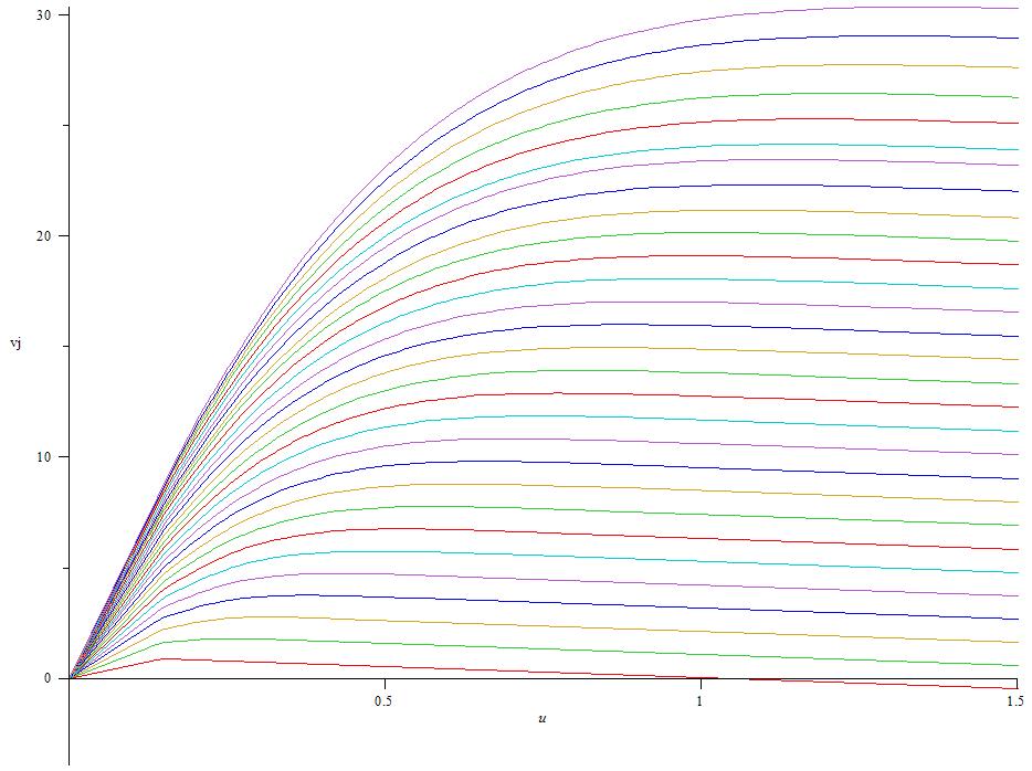
Figure 1: Functions $v_{j}(u)$ for $j=2..30$.

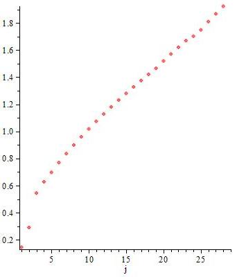
Figure 2: Values of $\gamma_{j}$ for $j=1..30$.

4 What happens when $r=0$?

In this section, we relax the assumption that the bank is impatient. A positive discount rate implies that there are gains from trades, as the bank is eager to sell claims on future cash flows to more patient investors. This is precisely what creates the moral hazard problem, as gains from trades can be undermined by high default rates when the bank shirks. We will see that, in contrast, the first-best is attained when $r=0$. Proofs are quite similar and only sketched. The analog of Proposition 3 is as follows.

Proposition 6

Assume that $r=0$.

• The ordinary differential equations (28), along with (27), have unique maximal solutions $v_{j}$ for $j\geq 1$. The functions $v_{j}$ are globally concave, differentiable everywhere except at $b_{j}$ and twice differentiable everywhere except at $b_{j}$ and $b_{j}+b_{j-1}$. The endogenous thresholds $\gamma_{j}$ are uniquely determined by

  $$\gamma_{j}=\frac{jB}{\epsilon\overline{\alpha}_{j}}.$$ (41)

• We also have

  $$v_{j}^{\prime}(u)-v_{j-1}^{\prime}(u-b_{j})\leq 0,\text{ for all }u\geq b_{j}.$$ (42)

Proof. $\mathrm{(i)}$ When $r=0$, the solution of (28) for a given $\gamma\geq b_{j}$ is

$$v_{j}(u) =\frac{j\mu}{\lambda_{j}}+e^{\frac{u-\gamma}{b_{j}}}\left(v_{j-1}(\gamma-b_{j})-b_{j}\right)+\int_{u}^{\gamma}\frac{e^{\frac{u-x}{b_{j}}}}{b_{j}}v_{j-1}(x-b_{j})dx,\text{ }b_{j}<u\leq\gamma$$ (43)

$$v_{j}(u) =\gamma-u+v_{j}(\gamma),\text{ }u>\gamma.$$

Using the same arguments as in the proof of Proposition 3, it is easily proved that the choice of $\gamma$ leading to the maximum solution is

$$\gamma_{j}=\gamma_{j-1}+b_{j}.$$

Reasoning by induction, we can then prove similarly that the functions $v_{j}$ verify all the desired properties. Moreover, since $\gamma_{1}=b_{1}$, we obtain that

$$\gamma_{j}=\sum_{i=1}^{j}b_{i}=\frac{jB}{\epsilon\overline{\alpha}_{j}}.$$

$\mathrm{(ii)}$ We can prove that

$$v_{j}^{\prime}(u) =\int_{u}^{\gamma_{j}}\frac{e^{\frac{u-x}{b_{j}}}}{b_{j}}\frac{dv_{j-1}}{du}(x-b_{j})dx-e^{\frac{u-\gamma_{j}}{b_{j}}},\text{ }b_{j}<u\leq\gamma_{j}$$

$$\frac{dv_{j}}{du}(u) =-1,\text{ }u>\gamma_{j}.$$

By the concavity of $v_{j-1}$, this implies that for $b_{j}<u\leq\gamma_{j}$

$$v_{j}^{\prime}(u)-v_{j-1}^{\prime}(u-b_{j})\leq-e^{\frac{u-\gamma_{j}}{b_{j}}}\left(v_{j-1}^{\prime}(u-b_{j})+1\right)\leq 0.$$

Since (42) is clear when $u>\gamma_{j}$, this proves $\mathrm{(ii)}$. $\Box$

Thanks to Proposition 6, we have a concave solution of the HJB equation, then using the same techniques as in the case $r>0$, we can verify that the optimal contract is given by

Contract 4.1

When $r=0$, the optimal contract can be described as follows:

• If, at some point, $u_{t}=\gamma_{j}$, there is no longer any stochastic liquidation. Fees are paid continuously to the bank, until extinction of the pool, at the rate $\delta_{t}^{i}=iB/\epsilon$ for all $i\leq j$.

• Otherwise, the policy is the same as in contract 3.1 (with $r=0$).

When the bank starts with reservation utility $\gamma_{I}$ (which is the market outcome when investors are competitive), payments are never suspended since the bank always operates at the thresholds $\gamma_{j}$ where payments are made. Hence, there can be no stochastic liquidation. More specifically, we have

$$v_{j}(\gamma_{j})=\frac{j\mu}{\lambda_{j}}-b_{j}+v_{j-1}(\gamma_{j-1}),$$

implying that the social value of the contract is

$$\gamma_{I}+v_{I}(\gamma_{I})=\gamma_{I}+\frac{I}{\overline{\alpha}_{I}}\left(\mu-\frac{B}{\epsilon}\right)=\frac{I\mu}{\overline{\alpha}_{I}}.$$

But according to (6) this is the social value attained in the first-best. Hence, when the bank is infinitely patient, the first-best is attained. For each $j$, the bank captures the maximum value of its rent, $\sum_{\left\{i\leq j\right\}}b_{i}$, but this is not socially costly since there is no loss arising from any “rent-preserving” fee.

Note that, to make the problem interesting, we have assumed that investments are not self-financing. Otherwise, the bank would be free to invest arbitrarily large amounts and there would be no demand for investors’ liquidity. This means that

$$v_{I}(\gamma_{I})<I.$$ (44)

In the general case, such a condition is difficult to work out, but when $r=0$ it is easily shown to be

$$\mu-\frac{B}{\varepsilon}<\overline{\alpha}_{I}.$$

This yields a lower bound for $B$. The moral hazard problem has to be severe enough that there is a funding problem. In the general case, we expect that the equivalent of (44) is going to hold for some lower bound on $B$ (which will depend on $r$).

Annexe A Appendix

Proof (Proof of Proposition 2)

In this particular case, Problem (9) becomes

$$v_{1}(u)=\sup_{D}\mathbb{E}^{\mathbb{P}}\left[\int_{0}^{\tau}\mu\,dt-dD_{t}\right]$$ (45)

subject to $$\mathbb{E}^{\mathbb{P}}\left[\int_{0}^{\tau}e^{-rt}\,dD_{t}\right]\geq u$$

$$u_{t}\geq b_{1},\text{ for all }t<\tau.$$

Consider first the subproblem derived from (45) by abstracting from the initial payment $D_{0}$ and ignoring the incentive compatibility constraint $u_{t}\geq b_{1}$:

$$\widetilde{v}_{1}(u)=\sup_{D}\mathbb{E}^{\mathbb{P}}\left[\int_{0+}^{\tau}\mu\,dt-dD_{t}\right]$$

subject to $$\mathbb{E}^{\mathbb{P}}\left[\int_{0+}^{\tau}e^{-rt}\,dD_{t}\right]\geq u.$$

The constraint can be written equivalently

$$\mathbb{E}^{\mathbb{P}}\left[\int_{0^{+}}^{\tau}e^{-rt}\left(dD_{t}-(r+\lambda_{1})u\,dt\right)\right]\geq 0.$$

The corresponding Lagrangian is

$$\mathcal{L}_{t}=\mu\,dt-dD_{t}+\nu_{t}e^{-rt}\left(dD_{t}-u(r+\lambda_{1})\,dt\right),$$

where $\nu_{t}$ is the Lagrange multiplier at time $t$. Optimizing with respect to $D$, we get $\nu_{t}=e^{rt}$ and the complementary slackness conditions imply that the dividend process is absolutely continuous and constant, namely $dD_{t}=\delta_{t}\,dt$, with $\delta_{t}=(r+\lambda_{1})u$. Since the process $D$ thus obtained is clearly admissible, this yields $\widetilde{v}_{1}(u)=\left(\mu-(r+\lambda_{1})u\right)/\lambda_{1}$.

Turning now to (45), but still ignoring the incentive compatibility constraint, we have

$$v_{1}(u)=\sup_{D_{0}}-D_{0}+\widetilde{v}_{1}(u-D_{0}),$$

which is increasing in $D_{0}$ when $r>0$. Since $u_{0}=u-D_{0}$ from the bank’s promise-keeping constraint (13), the highest initial payment consistent with the incentive compatibility constraint at time 0 is $D_{0}=u-b_{1}$. This yields

$$v_{1}(u) = b_{1}-u+\widetilde{v}_{1}(b_{1})$$

$$= b_{1}-u+\overline{v}_{1},$$

where $\overline{v}_{1}$ is defined as in the Proposition. Finally, one verifies that $\delta_{t}=b_{1}(r+\lambda_{1})$ yields $u_{t}=b_{1}$ on $\left[0,\tau\right)$, so that the incentive compatibility condition binds at all times before default, as desired.