Abstract

We propose a lattice model for two-dimensional $SU(N)$ $\mathcal{N}=(2,2)$ super Yang-Mills model. We start from the CKKU model for this system, which is valid only for $U(N)$ gauge group. We give a reduction of $U(1)$ part keeping a part of supersymmetry. In order to suppress artifact vacua, we use an admissibility condition.

1 Introduction

Supersymmetric gauge theories play an important role in both phenomenological and purely theoretical aspects. It is very natural to try to find a way to define supersymmetric theories nonperturbatively: a lattice regularization is a nice candidate. There have been proposed several approaches to the lattice regularization of supersymmetric Yang-Mills theories in the past decade (For reviews see [1, 2], for example). Most of them possess at least one exact supertransformation, which has an interpretation of a scalar supercharge in terms of topological twist. The supersymmetry (SUSY) algebra contains infinitesimal translations but the lattice allows only finite translations: the SUSY algebra needs to be represented by the finite translation. The (full) SUSY is broken at the finite lattice spacing, without introducing non-standard properties such as non-locality [3, 4].

In two dimensions the above mentioned exact scalar symmetry is strong enough to guarantee a restoration of full supersymmetry without fine tuning [8], which was explicitly checked in Monte Carlo simulations [9] for a model by Sugino [10]. In one dimension, a non-lattice approach without any exact supersymmetry at finite cutoff provides fine tuning free regularization [11]. Other fine tuning free lattice/non-lattice models for gauge theories are found in [12, 13, 14, 15, 16].

It is interesting to note that some of the known lattice formulations treat fermions as link variables. Since the gauge fields are treated as link variables on the lattice, it is quite natural to introduce fermions on links as superpartner of bosonic link variables. Here we focus on a 2-dimensional $\mathcal{N}=(2,2)$ system, which is the well studied system on the lattice. A Model proposed in [17] (CKKU model) was derived from a matrix model by using orbifolding, which naturally gives fermionic link variables. A geometrical approach [18] also uses link fermions. In [19], the present author together with his collaborators tried to introduce supercharges on links as well (link approach). The link approach originally intended to keep the full exact supersymmetry on the lattice at finite lattice spacing, but was turned out to be equivalent to the CKKU model [20]. On the other hand, a model proposed by Sugino (Sugino model), which also keeps the exact scalar supercharge, treat the fermion as site variables [21, 10, 22]. Both the CKKU model and the Sugino model describe the same target system in the continuum limit. In fact, both models give the same numerical results [23]. See [24, 22, 25, 26] for other approaches to this system and relation among the formulations, and [27, 28] for recent numerical studies. Note that this system is a 2-dimensional cousin of 4-dimensional $\mathcal{N}=4$ system in terms of Dirac-Kähler twist [29, 30].

There are two types of topological twist in 2-dimensional $\mathcal{N}=(2,2)$ systems and CKKU and Sugino models use different ones. They are called A-model twist and B-model twist. A-model twist combines the spacetime rotation and the internal $U(1)_{V}$ rotation. B-model uses the internal $U(1)_{A}$ instead of $U(1)_{V}$. CKKU model uses B-model twist and Sugino model uses A-model twist. We list further differences between the two formulations in Table 1.

	Sugino	CKKU
twist	A-model	B-model
fermion	site	link
gauge group	$U(N)$ or $SU(N)$	$U(N)$ only
admissibility	needed	no need

Table 1: Comparison of the Sugino model and the CKKU model.

In pure $U(N)$ super Yang-Mills theory without any matter multiplets, the $U(1)$ part of the gauge group is decoupled from the other part of the dynamics. However, in the CKKU model, due to the lattice artifacts the decoupling is not complete at finite lattice spacing. The CKKU model allows only $U(N)$ gauge group by construction and in fact a naive reduction to $SU(N)$ by hand does not work (see Sec. 3). The coupling with the $U(1)$ part may cause a fake sign problem as well [23]. Another, and more crucial problem of the $U(1)$ part of CKKU model is a stability of the $U(1)$ part of the scalar field. Because its expectation value gives the lattice spacing, the stability is quite important. An early analysis on this issue is found in [31]. In Monte Carlo simulations, an ad hoc treatment might be needed to stabilize it. One practical way is to introduce a mass term specific to the $U(1)$ part [23]. On the other hand, the Sugino model with $SU(N)$ gauge group is free from these problems. The cost we have to pay for the Sugino model is an admissibility condition, which is needed to suppress unphysical artifact vacua. The action is thus more complicated than that of CKKU model and an implementation of the model for numerical simulation becomes more complicated as well.

Motivated by the simpler implementation but the rather complicated treatment of $U(1)$ part of the CKKU model, in this paper, we propose an $SU(N)$ version of CKKU model. As we will describe, the obtained model is rather close to the Sugino model. Because link fermions require $U(N)$ gauge group, we need to use site fermions. In order to suppress artifact vacua we need the admissibility conditions as well. Unfortunately, because of the admissibility condition, the action becomes complicated.

In the next section we give a brief review of the CKKU model which uses $U(N)$ gauge group. Then we reduce the gauge group to $SU(N)$ in Sec. 3. The (classical) vacuum structure is analyzed in Sec. 4, which is needed for the admissibility condition. Sec. 5 contains conclusions and discussions.

2 A Brief Review of the $U(N)$ Model

In this section we give a brief review of the lattice model introduced in [17] and settle the notations. The target system is 2-dimensional $\mathcal{N}=(2,2)$ super Yang-Mills theory. We do not follow the original derivation with orbifolding and deconstruction but put emphasis on the nilpotent $Q$-symmetry.

We denote complex boson fields, which are made of gauge fields and scalar fields, as $\mathcal{U}_{\mu}$ and $\,\overline{\mathcal{U}}_{\mu}(=\mathcal{U}_{\mu}^{\dagger})$. We set all fields dimensionless. They live on links and their gauge transformations are

$$\mathcal{U}_{\mu}(n)\rightarrow G(n)\mathcal{U}_{\mu}(n)G^{-1}(n+\hat{\mu}),$$ (2.1)

where $G(n)$ is a group element of the gauge group, $n$ is a lattice site, and $\hat{\mu}$ is a unit vector in $\mu$-th direction. A bosonic auxiliary field $d$ is assigned to sites so transforms as site variable:

$$d(n)\rightarrow G(n)d(n)G^{-1}(n).$$ (2.2)

Fermions $\alpha,\ \beta,\ \xi$ are also assigned to links and $\lambda$ is to sites, so the gauge transformation reads:

$$\alpha(n) \rightarrow G(n)\alpha(n)G^{-1}(n+\hat{1}),$$ (2.3)

$$\beta(n) \rightarrow G(n)\beta(n)G^{-1}(n+\hat{2}),$$ (2.4)

$$\xi(n) \rightarrow G(n+\hat{1}+\hat{2})\xi(n)G^{-1}(n),$$ (2.5)

$$\lambda(n) \rightarrow G(n)\lambda(n)G^{-1}(n).$$ (2.6)

See Fig. 1. In terms of topological twist they are in the twisted basis: $\alpha$ and $\beta$ make a 2-dimensional vector, $\xi$ is an anti-symmetric tensor (i.e., a pseudo scalar in two dimensions), and $\lambda$ is a scalar.

Figure 1: Fields on the lattice for the CKKU model: fermions (left) and bosons (right).

They transform under a fermionic transformation $Q$, which is a scalar part of the twisted supersymmetry, in the following way:

$$Q\mathcal{U}_{1}(n) =2\alpha(n),\qquad Q\alpha(n)=0,$$ (2.7)

$$Q\mathcal{U}_{2}(n) =2\beta(n),\qquad Q\beta(n)=0,$$ (2.8)

$$Q\,\overline{\mathcal{U}}_{1}(n) =Q\,\overline{\mathcal{U}}_{2}(n)=0,$$ (2.9)

$$Q\lambda(n) =-\frac{1}{2}\Bigl{(}\,\overline{\mathcal{U}}_{1}(n-\hat{1})\mathcal{U}_{1}(n-\hat{1})-\mathcal{U}_{1}(n)\,\overline{\mathcal{U}}_{1}(n)$$

$$\qquad+\,\overline{\mathcal{U}}_{2}(n-\hat{2})\mathcal{U}_{2}(n-\hat{2})-\mathcal{U}_{2}(n)\,\overline{\mathcal{U}}_{2}(n)\Bigr{)}-id(n)$$

$$=-\frac{1}{2}\left([\,\overline{\mathcal{U}}_{1},\mathcal{U}_{1}]^{\prime}(n,n)+[\,\overline{\mathcal{U}}_{2},\mathcal{U}_{2}]^{\prime}(n,n)\right)-id(n),$$ (2.10)

$$Qd(n) =i\left(\,\overline{\mathcal{U}}_{1}(n-\hat{1})\alpha(n-\hat{1})-\alpha(n)\,\overline{\mathcal{U}}_{1}(n)\right)+i\left(\,\overline{\mathcal{U}}_{2}(n-\hat{2})\beta(n-\hat{2})-\beta(n)\,\overline{\mathcal{U}}_{2}(n)\right)$$

$$=i\left([\,\overline{\mathcal{U}}_{1},\alpha]^{\prime}(n,n)+[\,\overline{\mathcal{U}}_{2},\beta]^{\prime}(n,n)\right),$$ (2.11)

$$Q\xi(n) =\,\overline{\mathcal{U}}_{1}(n+\hat{2})\,\overline{\mathcal{U}}_{2}(n)-\,\overline{\mathcal{U}}_{2}(n+\hat{1})\,\overline{\mathcal{U}}_{1}(n)$$

$$=[\,\overline{\mathcal{U}}_{1},\,\overline{\mathcal{U}}_{2}]^{\prime}(n+\hat{1}+\hat{2},n).$$ (2.12)

Here we have introduced a shifted commutator

$$[A,B]^{\prime}(n,m)\equiv A(n,n+a_{A})B(n+a_{A},m)-B(n,n+a_{B})A(n+a_{B},m),$$ (2.13)

where $n+a_{A}+a_{B}=m$ and the locations of $A$ and $B$ are shifted to keep the gauge covariance (see Fig. 2). Their gauge transformations are

$$A(n,n_{A}) \rightarrow G(n)A(n,n_{A})G^{-1}(n_{A}), B(n,n_{B}) \rightarrow G(n)B(n,n_{B})G^{-1}(n_{B}),$$ (2.14)

respectively. The argument $(n,m)$ refers to the starting and end point of the link and the shifted commutator transforms as

$$[A,B]^{\prime}(n,m)\rightarrow G(n)[A,B]^{\prime}(n,m)G^{-1}(m).$$ (2.15)

It is easy to check that the above $Q$-transformation is nilpotent ($Q^{2}=0$).

Figure 2: A shifted commutator $[\mathcal{U}_{1},\mathcal{U}_{2}]^{\prime}(n,n+\hat{1}+\hat{2})=\mathcal{U}_{1}(n)\,\mathcal{U}_{2}(n+\hat{1})-\mathcal{U}_{2}(n)\,\mathcal{U}_{1}(n+\hat{2})$.

The action is given in a $Q$-exact form:

$$S_{U(N)}=Q\Lambda_{U(N)}$$ (2.16)

with preaction

$$\Lambda_{U(N)} =\kappa\sum_{n}\mathop{\mathrm{tr}}\nolimits\Bigl{[}-\frac{1}{4}\lambda(n)\left\{[\,\overline{\mathcal{U}}_{1},\mathcal{U}_{1}]^{\prime}(n,n)+[\,\overline{\mathcal{U}}_{2},\mathcal{U}_{2}]^{\prime}(n,n)-2id(n)\right\}$$

$$\qquad-\frac{1}{2}\xi(n)[\,\mathcal{U}_{1},\mathcal{U}_{2}]^{\prime}(n,n+\hat{1}+\hat{2})\Bigr{]}$$

$$=\kappa\sum_{n}\mathop{\mathrm{tr}}\nolimits\Bigl{[}\frac{1}{2}\lambda(n)\bigl{(}Q\lambda(n)\bigr{)}^{\dagger}+\frac{1}{2}\xi(n)\bigl{(}Q\xi(n)\bigr{)}^{\dagger}\Bigr{]}.$$ (2.17)

Because of the nilpotency, the invariance under the $Q$-transformation is manifest. Note that from the last expression the bosonic part of the action is positive (semi-)definite. The overall factor $\kappa$ is given as

$$\kappa=\frac{1}{g^{2}a^{2}}=\frac{N}{\lambda a^{2}},$$ (2.18)

where $g$ is a dimensionful gauge coupling, $\lambda=g^{2}/N$ is a ’t Hooft coupling, and $a$ is the lattice spacing. Eq. (2.16) reproduces a continuum action with fermion in a twisted basis:

$$S_{\rm cont.} =\frac{1}{g^{2}}\int d^{2}x\mathop{\mathrm{tr}}\nolimits\Bigl{[}\frac{1}{4}F_{\mu\nu}^{2}+\frac{1}{2}\sum_{i=1,2}(D_{\mu}s_{i})^{2}-\frac{1}{2}[s_{1},s_{2}]^{2}+\frac{1}{2}d^{2}$$

$$\qquad-\lambda D_{1}\alpha-\lambda D_{2}\beta+\xi D_{1}\beta-\xi D_{2}\alpha+\lambda[s_{1},\alpha]+\lambda[s_{2},\beta]+\xi[s_{1},\beta]-\xi[s_{2},\alpha]\Bigr{]},$$ (2.19)

where we have expanded the bosonic link variables as

$$\mathcal{U}_{\mu} =1+iaA_{\mu}+as_{\mu}+\dots$$ (2.20)

and rescaled the dimensionless lattice fields $d\to a^{2}d$ and $(\alpha,\beta,\lambda,\xi)\to(a^{\frac{3}{2}}\alpha,a^{\frac{3}{2}}\beta,a^{\frac{3}{2}}\lambda,a^{\frac{3}{2}}\xi)$. The covariant derivative is $D_{\mu}=\partial_{\mu}+i[A_{\mu},\ \cdot]$ and the curvature is $F_{\mu\nu}=-i[D_{\mu},D_{\nu}]$. The continuum $Q$-transformation is the following:

$$QA_{1} =-i\alpha,\qquad Q\alpha=0,$$ (2.21)

$$QA_{2} =-i\beta,\qquad Q\beta=0,$$ (2.22)

$$Qs_{1} =\alpha,\qquad\qquad Qs_{2}=\beta,$$ (2.23)

$$Q\lambda =D_{1}s_{1}+D_{2}s_{2}-id,$$ (2.24)

$$Qd =-i[D_{1},\alpha]-i[D_{2},\beta]+i[s_{1},\alpha]+i[s_{2},\beta],$$ (2.25)

$$Q\xi =iF_{12}+[s_{1},s_{2}]-D_{1}s_{2}+D_{2}s_{1}.$$ (2.26)

The continuum action and $Q$-transformation are valid for both $U(N)$ and $SU(N)$ gauge group.

3 Reduction to $SU(N)$

A naive reduction of the gauge group from $U(N)$ to $SU(N)$ does not work because of the following argument. We assume that fermions are algebra valued. Consider a fermion $\alpha(n)$, which should be traceless in the $SU(N)$ case. However, since its gauge transformation is

$$\alpha(n)\rightarrow G(n)\alpha(n)G(n+\hat{1})^{-1},$$ (3.1)

it is no longer in general traceless after the transformation. For the bosonic link fields it is not the case if we identify it using the exponential function

$$\mathcal{U}_{\mu}=\exp(aiA_{\mu}+as_{\mu}),$$ (3.2)

where $A_{\mu}$ and $s_{\mu}$ are the traceless Hermitian gauge field and the scalar, respectively. Because of the traceless exponent the determinant of $\mathcal{U}_{\mu}$ is unity. Since the determinant of the gauge transformation $G(n)$ is unity, it does not change the determinant of $\mathcal{U}_{\mu}$ (see the gauge transformation (2.1) ). In other words, a natural expansion for the bosonic link fields for $SU(N)$ is not a linear one but the exponential. Note that in the leading order in $a$, (3.2) agrees with the linear parameterization $\mathcal{U}_{\mu}=1+iaA_{\mu}+as_{\mu}$ but cannot keep the traceless property of $A_{\mu}$ and $s_{\mu}$ under the gauge transformation.

Therefore we define fermions on sites in order to keep the traceless nature. We decompose the link fermion into a product of a site fermion and a link boson (see Fig. 3). First, we decompose $\alpha(n)$ and $\beta(n)$ into

$$\alpha(n) =\hat{\alpha}(n)\mathcal{U}_{1}(n), \beta(n) =\hat{\beta}(n)\mathcal{U}_{2}(n),$$ (3.3)

where the hat ($\hat{\ }$) fields are defined on the site and can be expanded in the $SU(N)$ algebra:

$$\hat{\alpha}(n) =\sum_{a}T^{a}\hat{\alpha}^{a}(n), \hat{\beta}(n) =\sum_{a}T^{a}\hat{\beta}^{a}(n).$$ (3.4)

Their gauge transformation is

$$\hat{\alpha}(n) \rightarrow G(n)\hat{\alpha}(n)G^{-1}(n), \hat{\beta}(n) \rightarrow G(n)\hat{\beta}(n)G^{-1}(n),$$ (3.5)

which is consistent with the transformation for $\alpha$, $\beta$ and $\mathcal{U}_{\mu}$. From the $Q$-transformations for $\mathcal{U}_{\mu}$, $\alpha$ and $\beta$, we obtain the $Q$-transformations for the hatted fields:

$$Q\hat{\alpha}(n) =2\hat{\alpha}(n)\hat{\alpha}(n), Q\hat{\beta}(n) =2\hat{\beta}(n)\hat{\beta}(n).$$ (3.6)

After the $Q$-transformation they are still traceless, because of the fermionic nature,

$$\hat{\alpha}(n)\hat{\alpha}(n) =\sum_{a,b}\hat{\alpha}^{a}(n)\hat{\alpha}^{b}(n)T^{a}T^{b}=\sum_{a,b}\hat{\alpha}^{a}(n)\hat{\alpha}^{b}(n)\frac{1}{2}[T^{a},T^{b}],$$ (3.7)

and the commutator of $SU(N)$ generators $[T^{a},T^{b}]$ being traceless. The nilpotency $Q^{2}\hat{\alpha}=Q^{2}\hat{\beta}=0$ follows from the fermionic nature of $Q$: $Q^{2}\hat{\alpha}=2(Q\hat{\alpha})\hat{\alpha}-2\hat{\alpha}(Q\hat{\alpha})=0$, for example.

It should be noted that the $Q$-transformations in eq. (3.6) are higher order terms in lattice spacing: they are order $a$ terms. Although they are non-linear form at finite lattice spacing, they give the same transformation as eqs.(2.21) and (2.22) in the continuum limit. This is the same feature as $Q$-transformation for the Sugino model.

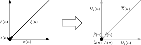
Figure 3: The link fermions (left) are decomposed into site fermions and link bosons (right).

We also introduce $\hat{\lambda}$, a traceless part of the scalar fermion $\lambda$. In order to keep it traceless, the $Q$-transformation should be

$$Q\hat{\lambda}(n)=-\frac{1}{2}\left\{[\,\overline{\mathcal{U}}_{1},\mathcal{U}_{1}]^{\prime}(n,n)+[\,\overline{\mathcal{U}}_{2},\mathcal{U}_{2}]^{\prime}(n,n)\right\}_{\rm t.l.}-i\hat{d}(n),$$ (3.8)

where we have also introduced a traceless auxiliary field $\hat{d}$ and $\rm t.l.$ refers to a traceless part

$$\{A\}_{\rm t.l.}\equiv A-\frac{1}{N}\mathop{\mathrm{tr}}\nolimits(A).$$ (3.9)

Note that the shifted commutator $[\,\cdot\,,\,\cdot\,]^{\prime}$ is not traceless. The gauge transformation for $\hat{\lambda}$ and $\hat{d}$ is a one for site variables:

$$\hat{\lambda}(n) \rightarrow G(n)\hat{\lambda}(n)G^{-1}(n), \hat{d}(n) \rightarrow G(n)\hat{d}(n)G^{-1}(n).$$ (3.10)

The $Q$-transformation of the auxiliary field $\hat{d}$ is obtained by requiring the nilpotency for $Q^{2}\hat{\lambda}=0$:

$$Q\hat{d}(n)=i\left\{[\,\overline{\mathcal{U}}_{1},\hat{\alpha}\mathcal{U}_{1}]^{\prime}(n,n)+[\,\overline{\mathcal{U}}_{2},\hat{\beta}\mathcal{U}_{2}]^{\prime}(n,n)\right\}_{\rm t.l.}\,.$$ (3.11)

Here we used the same transformation for $\,\overline{\mathcal{U}}_{\mu}$ as in the $U(N)$ case, $Q\,\overline{\mathcal{U}}_{\mu}=0$. We can show $Q^{2}\hat{d}=0$ as well.

The treatment of the diagonal-link fermion $\xi$ is non-trivial, because there is no diagonal-link boson. We define the traceless site fermion $\hat{\xi}$ and a diagonal link boson $\overline{\mathcal{D}}$ as

$$\xi(n)=\overline{\mathcal{D}}(n)\hat{\xi}(n).$$ (3.12)

Here we assume that $\overline{\mathcal{D}}$ is a function of $\,\overline{\mathcal{U}}_{\mu}$ thus $Q\overline{\mathcal{D}}=0$. The gauge transformation for these fields is

$$\overline{\mathcal{D}}(n) \rightarrow G(n+\hat{1}+\hat{2})\overline{\mathcal{D}}(n)G(n)^{-1}, \hat{\xi}(n) \rightarrow G(n)\hat{\xi}(n)G(n)^{-1}.$$ (3.13)

From eq. (2.12) we define the traceless $Q$ transformation of $\hat{\xi}$ as

$$Q\hat{\xi}(n) =\left\{\overline{\mathcal{D}}(n)^{-1}[\,\overline{\mathcal{U}}_{1},\,\overline{\mathcal{U}}_{2}]^{\prime}(n+\hat{1}+\hat{2},n)\right\}_{\rm t.l.}$$

$$=-i\left\{\overline{\mathcal{D}}(n)^{-1}\overline{\mathcal{F}}_{12}(n)\right\}_{\rm t.l.},$$ (3.14)

where we have introduced

$$i\mathcal{F}_{12}(n) =[\mathcal{U}_{1},\mathcal{U}_{2}]^{\prime}(n,n+\hat{1}+\hat{2}), i\overline{\mathcal{F}}_{12}(n) =[\,\overline{\mathcal{U}}_{1},\,\overline{\mathcal{U}}_{2}]^{\prime}(n+\hat{1}+\hat{2},n).$$ (3.15)

The $Q$-transformations are summarized in Appendix A.

In obtaining the action, we keep its $Q$-exact structure. It seems that it is just a rewriting of the preaction (2.17) in terms of site fermions. As we will see later, this is not a case with $\xi$, however.

The first term in (2.17) becomes

$$\Lambda^{(1)}_{SU(N)} \equiv\kappa\sum_{n}\mathop{\mathrm{tr}}\nolimits\Bigl{[}\frac{1}{2}\hat{\lambda}(n)\bigl{(}Q\hat{\lambda}(n)\bigr{)}^{\dagger}\Bigr{]}$$ (3.16)

and the contribution to the bosonic part of the action is

$$S^{(1)}_{SU(N)}\biggr{|}_{\rm Bosonic} =Q\Lambda^{(1)}_{SU(N)}\biggr{|}_{\rm Bosonic}$$

$$=\kappa\sum_{n}\Bigl{[}\frac{1}{8}\mathop{\mathrm{tr}}\nolimits\bigl{|}\left\{[\,\overline{\mathcal{U}}_{1},\mathcal{U}_{1}]^{\prime}(n,n)+[\,\overline{\mathcal{U}}_{2},\mathcal{U}_{2}]^{\prime}(n,n)\right\}_{\rm t.l.}\bigr{|}^{2}+\frac{1}{2}\mathop{\mathrm{tr}}\nolimits\hat{d}(n)^{2}\Bigr{]}.$$ (3.17)

One solution which gives the minimum of this term is unitary $\mathcal{U}_{\mu}$ and $\,\overline{\mathcal{U}}_{\mu}$ ($=\mathcal{U}_{\mu}^{\dagger}$), With the parameterization in eq. (3.2), the scalar fields $s_{\mu}$ are vanishing in this solution. Setting gauge fields $A_{\mu}$ zero and scalars constant, we also find another solutions, which is consistent with the fact that this term is a part of kinetic term of the scalar fields.

The second term of the preaction $\Lambda$ requires some care. The first candidate of a $SU(N)$ version is just a replacement of $\xi$ with $\overline{\mathcal{D}}\hat{\xi}$ in eq. (2.17):

$$\Lambda^{\prime(2)}_{SU(N)}=\kappa\sum_{n}\mathop{\mathrm{tr}}\nolimits\Bigl{[}\frac{1}{2}\mathcal{D}(n)\overline{\mathcal{D}}(n)\hat{\xi}(n)\bigl{(}Q\hat{\xi}(n)\bigr{)}^{\dagger}\Bigr{]},$$ (3.18)

where $\mathcal{D}=\overline{\mathcal{D}}^{\dagger}$ and we have used $Q\overline{\mathcal{D}}=0$. The bosonic action from this term is

$$S^{\prime(2)}_{SU(N)}\biggr{|}_{\rm Bosonic} =Q\Lambda^{\prime(2)}_{SU(N)}\biggr{|}_{\rm Bosonic}$$

$$=\kappa\sum_{n}\frac{1}{2}\mathop{\mathrm{tr}}\nolimits\left[\mathcal{D}(n)\overline{\mathcal{D}}(n)\left\{\overline{\mathcal{D}}(n)^{-1}\overline{\mathcal{F}}_{12}(n)\right\}_{\rm t.l.}\left\{\mathcal{F}_{12}(n)\mathcal{D}(n)^{-1}\right\}_{\rm t.l.}\right].$$ (3.19)

$\mathcal{F}_{12}\mathcal{D}^{-1}$ should be a function of the plaquette made of $\mathcal{U}_{\mu}$ and $\mathcal{U}_{\mu}^{-1}$ (but does not contain $\,\overline{\mathcal{U}}_{\mu}$ or $\,\overline{\mathcal{U}}_{\mu}^{-1}$). For simplicity, let us set the scalar fields $s_{\mu}$ to zero which gives a unitary plaquette. If the value of the plaquette belongs to a center of the gauge group, $\exp(\frac{2\pi i}{N}k)$ ($k=0,1,\dots,N-1$), its traceless part is always zero and gives a minimum of the action. Each of the plaquettes can have an arbitrary value in the center so the vacuum is highly degenerated. This is exactly the same situation found in a very first version of Sugino model [21]. The other part of the bosonic action (3.17) does not help to resolve this degeneracy.

In order to suppress the extra vacua, according to [10], we make use of an admissibility condition. We replace $\mathcal{D}\overline{\mathcal{D}}$ in the preaction (3.19) with a (divergent) function, and propose the following modification:

$$\Lambda^{(2)}_{SU(N)} =\kappa\sum_{n}\mathop{\mathrm{tr}}\nolimits\Bigl{[}\frac{1}{2}\frac{1}{1-\frac{1}{\epsilon^{2}}\frac{1}{N}||1-\mathcal{U}_{12}(n)||^{2}}\hat{\xi}(n)\bigl{(}Q\hat{\xi}(n)\bigr{)}^{\dagger}\Bigr{]},$$ (3.20)

where $\epsilon$ is a (small) number discussed in the next section,

$$\mathcal{U}_{12}(n)\equiv\mathcal{U}_{1}(n)\mathcal{U}_{2}(n+\hat{1})\mathcal{U}_{1}(n+\hat{2})^{-1}\,\mathcal{U}_{2}(n)^{-1}$$ (3.21)

and the squared norm of a matrix is

$$||A||^{2}\equiv\mathop{\mathrm{tr}}\nolimits(A^{\dagger}A).$$ (3.22)

Now the new action from $\Lambda^{(2)}_{SU(N)}$ becomes

$$S^{(2)}_{SU(N)}\biggr{|}_{\rm Bosonic} =Q\Lambda^{(2)}_{SU(N)}\biggr{|}_{\rm Bosonic}$$

$$=\kappa\sum_{n}\frac{1}{2}\mathop{\mathrm{tr}}\nolimits\left[\frac{1}{1-\frac{1}{\epsilon^{2}}\frac{1}{N}||1-\mathcal{U}_{12}(n)||^{2}}\left|\left\{\mathcal{F}_{12}(n)\mathcal{D}(n)^{-1}\right\}_{\rm t.l.}\right|^{2}\right].$$ (3.23)

Here we have written only the bosonic part and omitted the fermionic part. It is worth mentioning that neither $\mathcal{D}$ nor $\overline{\mathcal{D}}$ is needed any more in the action and the $Q$-transformation. What we need is only $\mathcal{D}^{-1}$ (and $\overline{\mathcal{D}}^{\,-1}$) and we assume that $-i\{\overline{\mathcal{D}}^{\,-1}(n)\overline{\mathcal{F}}_{12}(n)\}_{\rm t.l.}$ should go to the r.h.s of (2.26) in a continuum limit, because it is $Q\hat{\xi}$.

We further impose the admissibility condition so that the action is

$$S =\begin{cases}Q\left(\Lambda^{(1)}_{SU(N)}+\Lambda^{(2)}_{SU(N)}\right)\qquad&\frac{1}{N}||1-\mathcal{U}_{12}(n)||^{2}<\epsilon^{2},\\ \infty&\text{otherwise}.\end{cases}$$ (3.24)

Note that $||1-\mathcal{U}_{12}||=\mathcal{O}(a^{4})$ in a naive power counting. Therefore in a numerical simulation we expect that the admissibility condition is practically always satisfied if the simulation is close enough to the continuum limit. The explicit action with fermionic part after $Q$-transformation is given in Appendix A.

A possible variation of the action is to include $1/(1-\frac{1}{\epsilon^{2}}||1-\mathcal{U}_{12}||^{2})$ in $\Lambda^{(1)}_{SU(N)}$ as well. This makes the action more complicated but symmetric: terms from both $Q\Lambda^{(1)}_{SU(N)}$ and $Q\Lambda^{(2)}_{SU(N)}$ are equally complicated.

The measure for the path integral is invariant under the $Q$-transformation as well. A similar argument to [22] shows that

$$\left(\prod_{\mu}d[\mathcal{U}_{\mu}(n)]\right)d[\hat{d}(n)]\,d[\hat{\alpha}(n)]\,d[\hat{\beta}(n)]\,d[\hat{\lambda}(n)]\,d[\hat{\xi}(n)]$$ (3.25)

is the invariant measure. Here, $d[({\rm field})(n)]=\prod_{n}\prod_{a=1}^{N^{2}-1}d({\rm field})^{a}(n)$ for the auxiliary field $\hat{d}$ and fermions $\hat{\alpha},\hat{\beta},\hat{\lambda},\hat{\xi}$. The measure for complex gauge field $d[\mathcal{U}_{\mu}(n)]=\prod_{n}d\mathcal{U}_{\mu}(n)$ requires some care. We use the following parameterization (we suppress the suffix $\mu$ and lattice coordinate $n$)

$$\mathcal{U}=\exp(i\sum_{A=1}^{2N^{2}-2}X^{A}T^{A})\qquad(X^{A}:\text{real},\ \mathop{\mathrm{tr}}\nolimits(T^{A})=0).$$ (3.26)

Based on a similar argument to the standard Haar measure, we define

$$d\mathcal{U}=c\sqrt{\det(g_{AB}+g_{BA})}\prod_{A}dX^{A},$$ (3.27)

where

$$g_{AB}=\mathop{\mathrm{tr}}\nolimits\left[\mathcal{U}^{-1}\frac{\partial\mathcal{U}}{\partial X^{A}}\left(\mathcal{U}^{-1}\frac{\partial\mathcal{U}}{\partial X^{B}}\right)^{\dagger}\right]$$ (3.28)

and $c$ is a normalization constant. One can show that this measure is invariant under left-multiplication by a similar quantity, $\mathcal{V}=\exp(i\sum_{A=1}^{2N^{2}-2}Y^{A}T^{A})$. $Q$-transformation of $\mathcal{U}_{\mu}$ is this type of multiplication,

$$\mathcal{U}_{1} \to\mathcal{U}_{1}+i\varepsilon Q\mathcal{U}_{1}=\exp(2i\varepsilon\hat{\alpha})\mathcal{U}_{1}, \mathcal{U}_{2} \to\mathcal{U}_{2}+i\varepsilon Q\mathcal{U}_{2}=\exp(2i\varepsilon\hat{\beta})\mathcal{U}_{2}$$ (3.29)

with a grassmann parameter $\varepsilon$, so the measure is invariant under $Q$-transformation. In order to keep the invariance of (3.27) with the right-multiplication of $\mathcal{V}$, we need $\mathcal{V}\mathcal{V}^{\dagger}=1$. That is, only multiplication of a unitary matrix keeps the right-invariance of the measure. The gauge transformation, which is both right- and left- multiplications of unitary matrix, keeps the measure invariant. Note that in Monte Carlo simulations, updating of $\mathcal{U}_{\mu}$ is just a (left-) multiplying $\mathcal{V}$ as well so we do not need any measure term.

4 Detailed analysis on the Degenerate Vacua

In this section we give a bound for $\epsilon$ which appears in the admissibility condition. We need more information on $\mathcal{D}^{-1}$ so we restrict ourselves to the following case,

$$\mathcal{D}(n)^{-1}=t\,\mathcal{U}_{1}(n+\hat{2})^{-1}\,\mathcal{U}_{2}(n)^{-1}+(1-t)\,\mathcal{U}_{2}(n+\hat{1})^{-1}\,\mathcal{U}_{1}(n)^{-1},$$ (4.1)

where $0\leq t\leq 1$.

First we look for solutions of $\bigl{\{}i\mathcal{F}_{12}(n)\mathcal{D}(n)^{-1}\bigr{\}}_{\rm t.l.}=0$, which minimize (3.23). With our choice of $\mathcal{D}^{-1}$, we have

$$i\mathcal{F}_{12}(n)\mathcal{D}(n)^{-1}=1-2t+t\,\mathcal{U}_{12}(n)-(1-t)\bigl{(}\mathcal{U}_{12}(n)\bigr{)}^{-1}.$$ (4.2)

Then from the calculations given in Appendix B, we obtain the following solutions:

• $t=0$ or $t=1$: the center of $SU(N)$

  $$\mathcal{U}_{12}=\begin{pmatrix}e^{\frac{2\pi i}{N}n}&\\ &&\ddots\\ &&&e^{\frac{2\pi i}{N}n}\end{pmatrix}\qquad(n:\text{integer})$$ (4.3)

• $t\neq 0$ and $t\neq 1$:

  $$\mathcal{U}_{12}=\begin{pmatrix}e^{i\alpha+\beta}1_{k\times k}\\ &-\frac{1-t}{t}e^{-i\alpha-\beta}1_{(N-k)\times(N-k)}\end{pmatrix}$$ (4.4)

  with an integer $k\neq\frac{N}{2}$ and

  $$\alpha =\frac{N-k-2n}{N-2k}\pi\qquad(n:\text{integer}), e^{\beta}=\left(\frac{1-t}{t}\right)^{\frac{N-k}{N-2k}}.$$ (4.5)

  Setting $k=N$, we obtain the center of the $SU(N)$, which is unitary. As a special case $t=\frac{1}{2}$, we also obtain $e^{\beta}=1$ thus $\mathcal{U}_{12}$ is unitary.

• $t=\frac{1}{2}$ and $N=4m$: in addition to the above,

  $$\mathcal{U}_{12}=\begin{pmatrix}e^{i\alpha+\beta}1_{2m\times 2m}\\ &-e^{-i\alpha-\beta}1_{2m\times 2m}\end{pmatrix}$$ (4.6)

  with arbitrary real parameters $\alpha$ and $\beta$.

Then we look for the maximum allowed value for $\epsilon^{2}$. We use the admissibility condition

$$\frac{1}{N}||1-\mathcal{U}_{12}(n)||^{2}<\epsilon^{2}$$ (4.7)

for all the plaquette, and all solutions listed above need to violate this condition except for $\mathcal{U}_{12}(n)=1$ solution. Once one fixed $N$ and $t$, it is a straightforward task to find the maximum value of $\epsilon^{2}$ but is not easy to give a general form. Here we consider only $t=0,1$ and $\frac{1}{2}$ cases.

• $t=0$ or $t=1$. Substituting the center element (4.3) to the l.h.s of eq.(4.7), we obtain

  $$\frac{1}{N}||1-\mathcal{U}_{12}(n)||^{2}=4\sin^{2}\frac{n\pi}{N}.$$ (4.8)

  Because $n=0$ is the one we want to keep, i.e., $\mathcal{U}_{12}=1$, in order to suppress the unwanted vacua we should chose

  $$\epsilon^{2}\leq 4\sin^{2}\frac{\pi}{N}.$$ (4.9)

• $t=\frac{1}{2}$. The solution (4.4) gives

  $$\frac{1}{N}||1-\mathcal{U}_{12}(n)||^{2}=\frac{4(N-2k)}{N}\sin^{2}\frac{k-2n}{2(N-2k)}\pi+\frac{4k}{N}$$ (4.10)

  and a special case $N=4m$ (4.6) gives

  $$\frac{1}{N}||1-\mathcal{U}_{12}(n)||^{2}=2\left(\sinh\beta-\frac{1}{2}\cos\alpha\right)^{2}+2-\frac{1}{2}\cos^{2}\alpha\geq\frac{3}{2}.$$ (4.11)

  Noting a symmetry under $k\to N-k$ in (4.4), we obtain

  $$N =2 \epsilon^{2} \leq 4, (k=0,n=1)$$ (4.12)

  $$N =3 \epsilon^{2} \leq\frac{8}{3}, (k=1)$$ (4.13)

  $$N =4 \epsilon^{2} \leq\frac{3}{2}, (\text{from eq.(\ref{eq:sol-special2})})$$ (4.14)

  $$N \geq 5 \epsilon^{2} \leq 4\sin^{2}\frac{\pi}{N}, (k=0,n=1)$$ (4.15)

  where inside the parentheses indicates from which solution the bound for $\epsilon^{2}$ comes.

For large $N$, the bound for $\epsilon^{2}$ scales as $1/N^{2}$. This implies we need a finer lattice for larger $N$. We can estimate the scaling as follow. In a naive continuum limit, the action becomes

$$S\sim\frac{Na^{2}}{\lambda}\sum_{n}\sum_{a}(F_{12}^{a}(n))^{2}+\cdots,$$ (4.16)

where $F_{12}$ is a dimensionful gauge curvature and sum over color and coordinate indices are explicitly written. This gives the scaling

$$(F_{12}^{a}(n))^{2}\sim\frac{\lambda}{Na^{2}}$$ (4.17)

and thus

$$\frac{1}{N}||1-\mathcal{U}_{12}(n)||^{2}\sim\frac{a^{4}}{N}\sum_{a=1}^{N^{2}-1}(F_{12}^{a}(n))^{2}+\cdots\sim a^{2}\lambda.$$ (4.18)

Therefore the maximum lattice spacing should scale as

$$a^{2}\lambda\sim\frac{1}{N^{2}}$$ (4.19)

as $N$ becomes larger to satisfy the admissibility condition.

5 Conclusions and Discussions

We proposed a lattice action for $SU(N)$ $\mathcal{N}=(2,2)$ super Yang-Mills (3.24), starting with the CKKU model which has link fermions. Because fermions defined on the link cannot be $su(N)$ algebra valued, we decompose link fermions into site fermions and link bosons. We kept a nilpotent fermionic $Q$-transformation for these field at finite lattice spacing, which is a scalar part in terms of the topological twist. Using a fermionic nilpotent $Q$-transformation, we defined a $Q$-exact action. By construction the action enjoys $Q$-invariance manifestly. We encountered the degenerate vacua of the lattice model which does not capture the correct continuum physics. To suppress the artifact vacua, we used an admissibility condition. In Table 2 we summarize the feature of the model.

	Sugino	CKKU	$SU(N)$-CKKU
twist	A-model	B-model	B-model
fermion	site	link	site
gauge group	$U(N)$ or $SU(N)$	$U(N)$ only	$SU(N)$
admissibility	needed	no need	needed

Table 2: Comparisons of models.

A potential difficulty of CKKU model is a stability of $U(1)$ part of the scalar. In this paper, we removed the $U(1)$ part so there is no problem about the stability. However, due to the admissibility condition we introduced, the action became rather complicated. Removing the $U(1)$ part removed the problem with the stability of the $U(1)$ part of the scalar. We still need to take care of flat directions of the potential for the $SU(N)$ part of the scalar, by using large enough $N$ or a mass term, for example.

It is interesting to introduce matter multiplet to this model. A lattice model for 2-dimensional $\mathcal{N}=(2,2)$ supersymmetric QCD in [26] has similar degenerate vacua in the pure gauge sector, but they are resolved thanks to effects by the matter sector. The same thing might apply to our model.

Acknowledgements

The author thanks H. Suzuki and D. Kadoh for critical comments and discussions on the preliminary work. Discussions with F. Sugino were quite useful to complete this work. He also thanks F. Bruckmann, S. Catterall and M. Hanada. He thanks all the member of Theoretical Physics Laboratory in RIKEN and Okayama Institute for Quantum Physics for their hospitalities during his stay. Discussions at YITP Workshop “Field Theory and String Theory” (YITP-W-11-05) were useful to complete this work. The author is supported in part by the DFG SFB/Transregio 55 and acknowledges support from the EU ITN STRONGnet.

Appendix A Lattice Action

In this appendix, we give the explicit expression of the action (3.24):

$$S =\begin{cases}Q\left(\Lambda^{(1)}_{SU(N)}+\Lambda^{(2)}_{SU(N)}\right)\qquad&\frac{1}{N}||1-\mathcal{U}_{12}(n)||^{2}<\epsilon^{2},\\ \infty&\text{otherwise}.\end{cases}$$ (A.1)

$Q$-transformation given in Sec. 3 is

$$Q\mathcal{U}_{1}(n) =2\hat{\alpha}(n)\,\mathcal{U}_{1}(n),\qquad Q\hat{\alpha}(n)=2\hat{\alpha}(n)^{2},$$ (A.2)

$$Q\mathcal{U}_{2}(n) =2\hat{\beta}(n)\,\mathcal{U}_{2}(n),\qquad Q\hat{\beta}(n)=2\hat{\beta}(n)^{2},$$ (A.3)

$$Q\,\overline{\mathcal{U}}_{1}(n) =Q\,\overline{\mathcal{U}}_{2}(n)=0,$$ (A.4)

$$Q\hat{\lambda}(n) =-\frac{1}{2}\left\{\bigl{[}\,\overline{\mathcal{U}}_{1},\mathcal{U}_{1})\bigr{]}^{\prime}(n,n)+\bigl{[}\,\overline{\mathcal{U}}_{2},\mathcal{U}_{2})\bigr{]}^{\prime}(n,n)\right\}_{\rm t.l.}-i\hat{d}(n),$$ (A.5)

$$Q\hat{d}(n) =i\left\{\bigl{[}\,\overline{\mathcal{U}}_{1},\hat{\alpha}\mathcal{U}_{1}\bigr{]}^{\prime}(n,n)+\bigl{[}\,\overline{\mathcal{U}}_{2},\hat{\beta}\mathcal{U}_{2}\bigr{]}^{\prime}(n,n)\right\}_{\rm t.l.},$$ (A.6)

$$Q\hat{\xi}(n) =-i\left\{\overline{\mathcal{D}}(n)^{-1}\overline{\mathcal{F}}_{12}(n)\right\}_{\rm t.l.}.$$ (A.7)

The bosonic terms from $Q\Lambda_{SU(N)}^{(1)}$ and $Q\Lambda_{SU(N)}^{(2)}$ are given by eqs. (3.17) and (3.23), respectively:

$$S^{(1)}_{SU(N)}\biggr{|}_{\rm Bosonic} =\kappa\sum_{n}\Bigl{[}\frac{1}{8}\mathop{\mathrm{tr}}\nolimits\bigl{|}\left\{[\,\overline{\mathcal{U}}_{1},\mathcal{U}_{1}]^{\prime}(n,n)+[\,\overline{\mathcal{U}}_{2},\mathcal{U}_{2}]^{\prime}(n,n)\right\}_{\rm t.l.}\bigr{|}^{2}+\frac{1}{2}\mathop{\mathrm{tr}}\nolimits\hat{d}(n)^{2}\Bigr{]},$$ (A.8)

$$S^{(2)}_{SU(N)}\biggr{|}_{\rm Bosonic} =\kappa\sum_{n}\frac{1}{2}\mathop{\mathrm{tr}}\nolimits\left[\frac{1}{1-\frac{1}{\epsilon^{2}}\frac{1}{N}||1-\mathcal{U}_{12}(n)||^{2}}\left|\left\{\mathcal{F}_{12}(n)\mathcal{D}(n)^{-1}\right\}_{\rm t.l.}\right|^{2}\right].$$ (A.9)

The fermionic actions are

$$S^{(1)}_{SU(N)}\biggr{|}_{\rm Fermionic}=\kappa\sum_{n}\Bigl{[}\hat{\lambda}(n)[\,\overline{\mathcal{U}}_{1},\hat{\alpha}\mathcal{U}_{1}]^{\prime}(n,n)+\hat{\lambda}(n)[\,\overline{\mathcal{U}}_{2},\hat{\beta}\mathcal{U}_{2}]^{\prime}(n,n)\Bigr{]}$$ (A.10)

and

$$S^{(2)}_{SU(N)}\biggr{|}_{\rm Fermionic}=S_{\rm F}^{(2a)}+S_{\rm F}^{(2b)},$$ (A.11)

where

$$S_{\rm F}^{(2a)} =\kappa\sum_{n}\biggl{[}-\frac{1}{2}\frac{1}{1-\frac{1}{\epsilon^{2}}\frac{1}{N}||1-\mathcal{U}_{12}(n)||^{2}}\mathop{\mathrm{tr}}\nolimits\Bigl{[}\hat{\xi}(n)Q\Bigl{(}i\mathcal{F}_{12}(n)\mathcal{D}^{-1}(n)\Bigr{)}\Bigr{]}\biggr{]},$$ (A.12)

$$S_{\rm F}^{(2b)} =\kappa\sum_{n}\Biggl{[}\left(\frac{1}{1-\frac{1}{\epsilon^{2}}\frac{1}{N}||1-\mathcal{U}_{12}(n)||^{2}}\right)^{2}\mathop{\mathrm{tr}}\nolimits\Bigl{[}\hat{\xi}(n)\Bigl{(}i\mathcal{F}_{12}(n)\mathcal{D}^{-1}(n)\Bigr{)}\Bigr{]}$$

$$\qquad\times\frac{1}{\epsilon^{2}}\frac{1}{N}\mathop{\mathrm{tr}}\nolimits\Bigl{[}\Bigl{(}\mathcal{U}_{1}(n)\hat{\beta}(n+\hat{1})\mathcal{U}_{1}^{-1}(n)\mathcal{U}_{12}(n)-\mathcal{U}_{12}(n)\hat{\beta}(n)$$

$$\qquad\qquad-\mathcal{U}_{12}(n)\mathcal{U}_{2}(n)\hat{\alpha}(n+\hat{2})\mathcal{U}_{2}^{-1}(n)+\hat{\alpha}(n)\mathcal{U}_{12}(n)\Bigr{)}\Bigl{(}1-\,\overline{\mathcal{U}}_{12}(n)\Bigr{)}\Bigr{]}\Biggr{]}.$$ (A.13)

We need to specify $i\mathcal{F}_{12}(n)\mathcal{D}(n)^{-1}$ to calculate $Q$-transformation in $S_{\rm F}^{(2a)}$. Setting $i\mathcal{F}_{12}(n)\mathcal{D}(n)^{-1}$ as eq. (4.2),

$$i\mathcal{F}_{12}(n)\mathcal{D}(n)^{-1}=1-2t+t\,\mathcal{U}_{12}(n)-(1-t)\bigl{(}\mathcal{U}_{12}(n)\bigr{)}^{-1},$$ (A.14)

we obtain

$$S_{\rm F}^{(2a)} =\kappa\sum_{n}\frac{1}{1-\frac{1}{\epsilon^{2}}\frac{1}{N}||1-\mathcal{U}_{12}(n)||^{2}}$$

$$\qquad\times\biggl{\{}t\mathop{\mathrm{tr}}\nolimits\Bigl{[}\hat{\xi}(n)\Bigl{(}\mathcal{U}_{12}(n)\mathcal{U}_{2}(n)\hat{\alpha}(n+\hat{2})\mathcal{U}_{2}^{-1}(n)-\hat{\alpha}(n)\mathcal{U}_{12}(n)\Bigr{)}$$

$$\qquad\qquad-\hat{\xi}(n)\Bigl{(}\mathcal{U}_{1}(n)\hat{\beta}(n+\hat{1})\mathcal{U}_{1}^{-1}(n)\mathcal{U}_{12}(n)-\mathcal{U}_{12}(n)\hat{\beta}(n)\Bigr{)}\Bigr{]}$$

$$\qquad+(1-t)\mathop{\mathrm{tr}}\nolimits\Bigl{[}\hat{\xi}(n)\Bigl{(}\mathcal{U}_{2}(n)\hat{\alpha}(n+\hat{2})\mathcal{U}_{2}^{-1}(n)\mathcal{U}_{12}^{-1}(n)-\mathcal{U}_{12}^{-1}(n)\hat{\alpha}(n)\Bigr{)}$$

$$\qquad\qquad-\hat{\xi}(n)\Bigl{(}\mathcal{U}_{12}^{-1}(n)\mathcal{U}_{1}(n)\hat{\beta}(n+\hat{1})\mathcal{U}_{1}^{-1}(n)-\hat{\beta}(n)\mathcal{U}_{12}^{-1}(n)\Bigr{)}\Bigr{]}\biggr{\}}.$$ (A.15)

To obtain the above expressions, we dropped irrelevant trace less symbols ($\rm t.l.$) because of a relation $\mathop{\mathrm{tr}}\nolimits\bigl{[}\hat{\xi}(A)_{\rm t.l.}\bigr{]}=\mathop{\mathrm{tr}}\nolimits\bigl{[}\hat{\xi}A\bigr{]}$ for any $N\times N$ matrix $A$ and traceless $\hat{\xi}$.

Appendix B Solution of the equation of motion

We solve the following equation:

$$0=\left\{i\mathcal{F}_{12}(n)\mathcal{D}(n)^{-1}\right\}_{\rm t.l.}=\left\{t\,\mathcal{U}_{12}(n)-(1-t)\bigl{(}\mathcal{U}_{12}(n)\bigr{)}^{-1}\right\}_{\rm t.l.}\ .$$ (B.1)

We parameterize $\mathcal{U}_{12}$ as

$$\mathcal{U}_{12}(n)=\begin{pmatrix}e^{i\alpha_{1}+\beta_{1}}&&&0\\ &e^{i\alpha_{2}+\beta_{2}}\\ &&\ddots\\ 0&&&e^{i\alpha_{N}+\beta_{N}}\end{pmatrix},$$ (B.2)

with real parameters $\alpha_{i},\beta_{i}$ which satisfy $\sum_{i}\alpha_{i}=\sum_{i}\beta_{i}=0$. Denoting the diagonal component as

$$\lambda_{i} =te^{i\alpha_{i}+\beta}+(t-1)e^{-i\alpha_{i}-\beta_{i}}$$

$$=(te^{\beta_{i}}-(1-t)e^{-\beta_{i}})\cos\alpha_{i}+i(te^{\beta_{i}}+(1-t)e^{-\beta_{i}})\sin\alpha_{i}\equiv s_{i}\cos\alpha_{i}+ic_{i}\sin\alpha_{i},$$ (B.3)

we rewrite the solution of eq. (B.1) as

$$\lambda_{1}=\lambda_{2}=\dots=\lambda_{N}$$ (B.4)

which gives

$$\begin{cases}&s_{i}\cos\alpha_{i}=s_{j}\cos\alpha_{j}\\ &c_{i}\sin\alpha_{i}=c_{j}\sin\alpha_{j}\end{cases}$$ (B.5)

for $i,j=1,\dots,N$. Using $c_{i}^{2}-s_{i}^{2}=4t(1-t)$ and $c_{i}\leq 2\sqrt{t(1-t)}\sin\alpha_{i}$, we obtain

$$c_{i}\pm 2\sqrt{t(1-t)}\sin\alpha_{i}=c_{j}\pm 2\sqrt{t(1-t)}\sin\alpha_{j}.$$ (B.6)

This gives

$$\begin{cases}&c_{i}=c_{j}\\ &\sin\alpha_{i}=\sin\alpha_{j},\end{cases}$$ (B.7)

which is valid even with $t=0$ or $1$. (Note that $c_{i}\neq 0$ and eq. (B.5).) Consistent solutions with eq. (B.5) are

$$\alpha_{i}=\alpha_{j},\qquad\beta_{i}=\beta_{j}$$ (B.8)

or

$$\alpha_{i}=\pi-\alpha_{j},\qquad e^{\beta_{i}}=\frac{1-t}{t}e^{-\beta_{j}}.\qquad(t\neq 0,1)$$ (B.9)

Suppose we set $\alpha_{i}$ to

$$\alpha_{i}=(\underbrace{\alpha,\alpha,\dots,\alpha}_{k},\ \underbrace{\pi-\alpha,\dots\pi-\alpha}_{N-k})$$ (B.10)

and thus

$$\beta_{i}=(\underbrace{\beta,\beta,\dots,\beta}_{k},\ \underbrace{-\beta+\ln\frac{1-t}{t},\dots,-\beta+\ln\frac{1-t}{t}}_{N-k}),$$ (B.11)

where $0\leq k\leq N$. The additional condition from $SU(N)$ gives

$$0=\sum_{i=1}^{N}\beta_{i}=-(N-2k)\beta+(N-k)\ln\frac{1-t}{t},$$ (B.12)

and

$$2\pi m=\sum_{i=1}^{N}\alpha_{i}=-(N-2k)\alpha+(N-k)\pi,$$ (B.13)

where $m$ is an integer. We finally obtain

$$N \neq 2k: \alpha=\frac{N-k-2m}{N-2k}\pi,\quad\beta=\frac{N-k}{N-2k}\ln\frac{1-t}{t},$$ (B.14)

$$N =2k: \alpha,\beta\text{ are arbitrary},\ t=\frac{1}{2},\ N=4m,$$ (B.15)

which give eq. (4.4)–(4.6).

If $t=0$ or $1$, only $k=N$ is possible. The solution becomes the center of $SU(N)$:

$$\alpha_{i}=\frac{2\pi}{N}n,\quad\beta_{i}=0.$$ (B.16)

References

- [1] S. Catterall, D. B. Kaplan and M. Ünsal, Phys. Rept. 484 (2009) 71 [arXiv:0903.4881 [hep-lat]].
- [2] A. Joseph, Int. J. Mod. Phys. A 26 (2011) 5057 [arXiv:1110.5983 [hep-lat]].
- [3] M. Kato, M. Sakamoto and H. So, JHEP 0805 (2008) 057 [arXiv:0803.3121 [hep-lat]].
- [4] G. Bergner, JHEP 1001 (2010) 024 [arXiv:0909.4791 [hep-lat]].
- [5] D. Kadoh and H. Suzuki, Phys. Lett. B 684 (2010) 167 [arXiv:0909.3686 [hep-th]].
- [6] A. D’Adda, A. Feo, I. Kanamori, N. Kawamoto and J. Saito, JHEP 1009 (2010) 059 [arXiv:1006.2046 [hep-lat]].
- [7] A. D’Adda, I. Kanamori, N. Kawamoto and J. Saito, JHEP 1203 (2012) 043 [arXiv:1107.1629 [hep-lat]].
- [8] D. B. Kaplan, E. Katz and M. Ünsal, JHEP 0305 (2003) 037 [hep-lat/0206019].
- [9] I. Kanamori and H. Suzuki, Nucl. Phys. B 811 (2009) 420 [arXiv:0809.2856 [hep-lat]].
- [10] F. Sugino, JHEP 0403 (2004) 067 [arXiv:hep-lat/0401017].
- [11] M. Hanada, J. Nishimura and S. Takeuchi, Phys. Rev. Lett. 99 (2007) 161602 [arXiv:0706.1647 [hep-lat]].
- [12] M. Hanada, S. Matsuura and F. Sugino, Prog. Theor. Phys. 126 (2012) 597 [arXiv:1004.5513 [hep-lat]].
- [13] M. Hanada, JHEP 1011 (2010) 112 [arXiv:1009.0901 [hep-lat]].
- [14] M. Hanada, S. Matsuura and F. Sugino, Nucl. Phys. B 857 (2012) 335 [arXiv:1109.6807 [hep-lat]].
- [15] T. Ishii, G. Ishiki, S. Shimasaki and A. Tsuchiya, Phys. Rev. D 78 (2008) 106001 [arXiv:0807.2352 [hep-th]].
- [16] G. Ishiki, S. Shimasaki and A. Tsuchiya, JHEP 1111 (2011) 036 [arXiv:1106.5590 [hep-th]].
- [17] A. G. Cohen, D. B. Kaplan, E. Katz and M. Ünsal, JHEP 0308 (2003) 024 [arXiv:hep-lat/0302017].
- [18] S. Catterall, JHEP 0411 (2004) 006 [hep-lat/0410052].
- [19] A. D’Adda, I. Kanamori, N. Kawamoto and K. Nagata, Phys. Lett. B 633 (2006) 645 [arXiv:hep-lat/0507029].
- [20] P. H. Damgaard and S. Matsuura, JHEP 0709 (2007) 097 [arXiv:0708.4129 [hep-lat]].
- [21] F. Sugino, JHEP 0401 (2004) 015 [arXiv:hep-lat/0311021].
- [22] F. Sugino, Phys. Lett. B 635 (2006) 218 [arXiv:hep-lat/0601024].
- [23] M. Hanada and I. Kanamori, JHEP 1101 (2011) 058 [arXiv:1010.2948 [hep-lat]].
- [24] H. Suzuki and Y. Taniguchi, JHEP 0510 (2005) 082 [arXiv:hep-lat/0507019].
- [25] T. Takimi, JHEP 0707 (2007) 010 [arXiv:0705.3831 [hep-lat]].
- [26] D. Kadoh, F. Sugino and H. Suzuki, Nucl. Phys. B 820 (2009) 99 [arXiv:0903.5398 [hep-lat]].
- [27] S. Catterall and A. Joseph, Comput. Phys. Commun. 183 (2012) 1336 [arXiv:1108.1503 [hep-lat]].
- [28] S. Catterall, R. Galvez, A. Joseph and D. Mehta, JHEP 1201 (2012) 108 [arXiv:1112.3588 [hep-lat]].
- [29] N. Kawamoto and T. Tsukioka, Phys. Rev. D 61 (2000) 105009 [arXiv:hep-th/9905222].
- [30] J. Kato, N. Kawamoto and Y. Uchida, Int. J. Mod. Phys. A 19 (2004) 2149 [arXiv:hep-th/0310242].
- [31] T. Onogi and T. Takimi, Phys. Rev. D 72, 074504 (2005) [arXiv:hep-lat/0506014].
- [32] M. Ünsal, JHEP 0511 (2005) 013 [arXiv:hep-lat/0504016].
- [33] R. Galvez, S. Catterall, A. Joseph and D. Mehta, PoS LATTICE 2011 (2011) 064 [arXiv:1201.1924 [hep-lat]].
- [34] F. Sugino, private commnications.