Berkeley Supernova Ia Program II: Initial Analysis of Spectra Obtained Near Maximum Brightness

Abstract

In this second paper in a series we present measurements of spectral features of 432 low-redshift ($z<0.1$) optical spectra of 261 Type Ia supernovae (SNe Ia) within 20 d of maximum brightness. The data were obtained from 1989 through the end of 2008 as part of the Berkeley SN Ia Program (BSNIP) and are presented in BSNIP I (Silverman et al. 2012). We describe in detail our method of automated, robust spectral feature definition and measurement which expands upon similar previous studies. Using this procedure, we attempt to measure expansion velocities, pseudo-equivalent widths (pEW), spectral feature depths, and fluxes at the centre and endpoints of each of nine major spectral feature complexes. We investigate how velocity and pEW evolve with time and how they correlate with each other. Various spectral classification schemes are employed and quantitative spectral differences among the subclasses are investigated. Several ratios of pEW values are calculated and studied. The so-called Si ii ratio, often used as a luminosity indicator (Nugent et al. 1995), is found to be well correlated with the so-called “SiFe” ratio and anticorrelated with the analogous “SSi ratio,” confirming the results of previous studies. Furthermore, SNe Ia that show strong evidence for interaction with circumstellar material or an aspherical explosion are found to have the largest near-maximum expansion velocities and pEWs, possibly linking extreme values of spectral observables with specific progenitor or explosion scenarios. We find that purely spectroscopic classification schemes are useful in identifying the most peculiar SNe Ia. However, in almost all spectral parameters investigated the full sample of objects spans a nearly continuous range of values. Comparisons to previously published theoretical models of SNe Ia are made and we conclude with a brief discussion of how the measurements performed herein and the possible correlations presented will be important for future SN surveys.

1 Introduction

Type Ia supernovae (SNe Ia) have been particularly useful in recent years as a way to accurately measure cosmological parameters (e.g., Astier et al., 2006; Riess et al., 2007; Wood-Vasey et al., 2007; Hicken et al., 2009; Kessler et al., 2009; Amanullah et al., 2010; Suzuki et al., 2012), and led to the discovery of the accelerating expansion of the Universe (Riess et al., 1998; Perlmutter et al., 1999). Broadly speaking, SNe Ia are the result of thermonuclear explosions of C/O white dwarfs (WDs) (e.g., Hoyle & Fowler 1960; Colgate & McKee 1969; Nomoto et al. 1984; see Hillebrandt & Niemeyer 2000 for a review). However, we still lack a detailed understanding of the progenitor systems and explosion mechanisms, as well as how differences in initial conditions create the variance in observed properties of SNe Ia. To solve these problems, and others, detailed and self-consistent observations of many hundreds of SNe Ia are required.

The cosmological application of SNe Ia as precise distance indicators relies on being able to standardise their luminosity. Phillips (1993) showed that the light-curve decline rate is well correlated with luminosity at peak brightness for most SNe Ia, the so-called “Phillips relation.” However, this simple empirical relation relies on photometry alone, and it may be possible to refine the relation with the addition of spectral observations. Many comparisons of spectral features and studies of the temporal evolution of these features in low-redshift SN Ia have been performed in the past (e.g., Barbon et al., 1990; Branch & van den Bergh, 1993; Nugent et al., 1995; Hatano et al., 2000; Folatelli, 2004; Benetti et al., 2005; Bongard et al., 2006; Hachinger et al., 2006; Bronder et al., 2008; Foley et al., 2008; Branch et al., 2009; Wang et al., 2009; Walker et al., 2011; Nordin et al., 2011b; Blondin et al., 2011; Konishi et al., 2011; Foley & Kasen, 2011). In addition, there has been similar work with SNe Ia at higher redshifts (e.g., Hook et al., 2005; Blondin et al., 2006; Altavilla et al., 2009; Garavini et al., 2007; Bronder et al., 2008; Walker et al., 2011; Konishi et al., 2011). Many of these studies aimed to find a “second parameter” in SN Ia spectra which would make our measurements of the distances to SNe Ia even more precise.

However, most of these studies utilised relatively small and heterogeneous datasets or were hindered by low signal-to-noise ratio (S/N) data. Using the self-consistently observed and reduced low-redshift ($z\leq 0.2$) optical SN Ia spectra from the Berkeley Supernova Ia Program (BSNIP; Silverman et al., 2012), we can accurately and robustly measure various spectral features. These measurements can then be used to investigate how the spectral observables correlate with each other and with the objects’ previously determined spectral subclasses based on different classification schemes.

We provide an overview of the dataset used for this analysis in Section 2, and we describe in detail our automated and robust procedure for measuring multiple aspects of each spectral feature in Section 3. Our resulting measurements are described in Section 4. Section 5 presents the temporal evolution of these measured values, and how they correlate with each other and with previously determined spectral classifications. We discuss our conclusions in Section 6, specifically summarising the main results from our analysis in Section 6.1. Finally, we attempt to answer questions regarding whether theoretical models can explain the spectra of SNe Ia and the correlations we find (Section 6.2) and how our analysis of spectral features will be important for future SN surveys (Section 6.3). Forthcoming BSNIP papers will utilise the spectral measurements described here and examine the correlations between these and other observables (such as photometry and host-galaxy properties).

2 Spectral Dataset

The SN Ia spectra that are used in this study all come from BSNIP and are published in BSNIP I (Silverman et al., 2012). The majority of the spectra were obtained with the Shane 3 m telescope at Lick Observatory using the Kast double spectrograph (Miller & Stone, 1993). The typical wavelength coverage is 3300–10,400 Å with resolutions of $\sim\!\!$ 11 and $\sim\!\!$ 6 Å on the red and blue sides, respectively (crossover wavelength $\sim\!\!$ 5500 Å). As discussed in BSNIP I (Silverman et al., 2012) the sample contains spectra of all subtypes of SNe Ia in roughly the same proportions as what was analysed in Ganeshalingam et al. (2010), which is the companion photometric dataset to much of the BSNIP sample.

In BSNIP I (Silverman et al., 2012) it was shown that the relative spectrophotometric accuracy is $<0.1$ mag for the BSNIP data and only approaches 0.1 mag in the oldest and noisest spectra. On the other hand, the absolute spectrophometry is only correct in a handful of spectra. Thus, flux measurements alone may be inaccurate, but ratios of flux values should be quite precise. Some of the spectra examined here have had residual host-galaxy contamination removed using our “colour matching” technique. This method uses photometry of the host galaxy of a SN to correct for any contamination that remains after our normal data-reduction procedure (which often removes the majority of host-galaxy light). Further information regarding the observations, data reduction, spectrophotometric accuracy, and host-galaxy corrections can be found in BSNIP I.

For this study we required that a spectrum be within 20 d (rest frame) of maximum brightness, using the redshift and Julian Date of maximum presented in Table 1 of BSNIP I. The only SNe which we ignored a priori were the extremely peculiar SN 2000cx (e.g., Li et al., 2001), SN 2002cx (e.g., Li et al., 2003; Jha et al., 2006), SN 2005hk (e.g., Chornock et al., 2006; Phillips et al., 2007), and SN 2008ha (e.g., Foley et al., 2009; Valenti et al., 2009). After removing these objects, we were left with 458 spectra (147 of which were corrected for host-galaxy contamination) of 271 SNe Ia, and we attempted to measure their spectral features.

Of these, there were some spectra which did not pass our minimum S/N cut (see Section 3.3), or whose wavelength range did not sufficiently cover any of the features we wanted to measure (see Section 3.1). In addition, the endpoints of each feature sometimes fell outside our allowed boundaries (see Section 3.2), or every spectral feature that was measured was deemed to have a poorly defined continuum (see Section 3.6). After removing these data there remain 432 spectra of 261 SNe Ia with a “good” fit for at least one spectral feature. The largest redshift of these observations is $\sim\!\!$ 0.1 (even though the full BSNIP dataset contains SNe with $0.1<z<0.2$). The earliest spectrum successfully fit in this work has a rest-frame age of about $-12.7$ d. A summary of these SNe Ia, their ages, and spectral classifications based on various classification schemes can be found in Appendix A.

We consider an object “spectroscopically normal” if it is classified as “Ia-norm” by the SuperNova IDentification code (SNID; Blondin & Tonry, 2007) as implemented in BSNIP I. In the current study we have 213 Ia-norm objects and 5 “Ia” objects for which we were unable to determine a definitive subtype in BSNIP I. There are 24 SN 1991bg-like objects (“Ia-91bg,” e.g., Filippenko et al., 1992b; Leibundgut et al., 1993) which represent the usually underluminous SNe Ia. We also have 6 SN 1991T-like objects (“Ia-91T,” e.g., Filippenko et al., 1992a; Phillips et al., 1992) and 13 SN 1999aa-like objects (“Ia-99aa,” e.g., Li et al., 2001; Strolger et al., 2002; Garavini et al., 2004) which together represent the often overluminous SNe Ia. These classifications are listed in the “SNID (Sub)Type” column of Table LABEL:t:data. See BSNIP I for more information regarding our implementation of SNID and the various spectroscopic subtype classifications.

3 Measurement Procedure

3.1 Measured Features

Previous studies similar to this one have split optical SN Ia spectra near maximum brightness into eight or nine major absorption feature complexes (e.g., Riess et al., 1997; Folatelli, 2004; Hachinger et al., 2006). All of these are features are actually blends of multiple spectral transitions, but each absorption complex itself is often distinct enough from the others for its properties to be measured independently. We follow previous studies’ naming convention for the measured features by referring to each one by an ion or spectral line responsible for the majority of the absorption. The nine features we attempt to fit in each observation are labelled on a spectrum of the “normal” Type Ia SN 2002ha (taken 1 d before maximum brightness) in Figure 1. Each feature’s name and reference number, along with its rest wavelength (used to determine expansion velocities), is presented in Table 1.

Figure 1: The nine features we attempt to fit in each observation shown on a spectrum of the “normal” Type Ia SN 2002ha, taken 1 d before maximum brightness, from BSNIP I. The spectrum has had its host-galaxy recession velocity removed and has been corrected for Milky Way reddening according to the values presented in Table 1 of BSNIP I and assuming that the extinction follows the Cardelli et al. (1989) extinction law modified by O’Donnell (1994). See Table 1 for more information regarding each feature.

Table 1: Spectral Features and Boundaries

Feature Name	Feature #	Rest Wavelength${}^{\textrm{a}}$ (Å)	Blue Boundary${}^{\textrm{b}}$ (Å)	Red Boundary${}^{\textrm{b}}$ (Å)
Ca ii H&K	f1	3945.28	3400–3800	3800–4100
Si ii $\lambda$4000	f2	4129.73	3850–4000	4000–4150
Mg ii	f3	$\cdots$${}^{\textrm{c}}$	4000–4150	4350–4700
Fe ii	f4	$\cdots$${}^{\textrm{c}}$	4350–4700	5050–5550
S ii “W”${}^{\textrm{d}}$	f5	5624.32	5100–5300	5450–5700
Si ii $\lambda$5972	f6	5971.85	5400–5700	5750–6000
Si ii $\lambda$6355	f7	6355.21	5750–6060	6200–6600
O i Triplet	f8	7773.37	6800–7450	7600–8000
Ca ii Near-IR Triplet	f9	8578.75	7500–8100	8200–8900
${}^{\textrm{a}}$The rest wavelengths are weighted averages of the strongest spectral lines that give rise to each absorption feature.
${}^{\textrm{b}}$These boundaries are necessary in order to account for variations in spectral feature width and expansion velocity among SNe, as well as the temporal evolution of these values.
${}^{\textrm{c}}$This feature is a blend of so many spectral lines that a single reference wavelength is practically meaningless (and thus an expansion velocity cannot be accurately determined).
${}^{\textrm{d}}$The two broad absorptions that make up the S ii “W” are fit using a single spline, but we calculate the expansion velocity of the absorption complex using the minimum of the redder of the two features relative to its rest wavelength.

There have been a significant number of spectroscopically peculiar SNe Ia observed whose spectra near maximum brightness do not contain some of the nine features or exhibit extremely weak absorptions from certain features (for a review of these objects, see Filippenko, 1997). These are the peculiar subtypes discussed at the end of Section 2 and classified in the current analysis using SNID. We include these peculiar objects in our study in an attempt to better quantify the extent of the spectral peculiarities among these types of SNe Ia. However, as mentioned in Section 2, there are some objects which are so spectroscopically peculiar (compared with “normal” SNe Ia) that we have removed them from our sample.

3.2 Allowed Boundaries

As in previous studies, we require that the endpoints for each feature, as determined on a SN-by-SN basis by our fitting algorithm (see Section 3.4), be within predetermined boundaries (e.g., Folatelli, 2004; Nordin et al., 2011b). These boundaries allow the fitting routine to make sure that we are considering only a single feature at a time and not also including a neighbouring feature. The size of these boundaries is necessary to account for variations in spectral feature width and expansion velocity among SNe, as well as the temporal evolution of these values. Even though the formal boundaries of neighboring features (among the totality of SN spectra) may overlap, the actual endpoints of neighboring features in a given spectrum will not. We also note that not every pixel in every spectrum will be part of a feature; some will effectively correspond to “continuum” flux.

The boundaries used here are slightly modified from those in previous studies; our boundaries tend to be wider than those of our predecessors (e.g., Folatelli, 2004; Nordin et al., 2011b). The final values of our boundaries were a result of extensive testing and represent a compromise between including as many fits as possible (by accounting for differences in spectral feature width and velocity) while making sure that no endpoints overlap with a neighboring feature. The boundaries used in this work for each spectral feature can be found in Table 1.

3.3 Initial Steps

For each spectrum we begin by removing the host-galaxy recession velocity and correcting for Milky Way (MW) reddening according to the values presented in Table 1 of BSNIP I and assuming that the extinction follows the Cardelli et al. (1989) extinction law modified by O’Donnell (1994). The spectrum is then smoothed using a Savitzky-Golay smoothing filter (Savitzky & Golay, 1964). By smoothing each spectrum we can effectively remove errant flux values in individual pixels (or pairs of consecutive pixels) due to, for example, cosmic rays. Measured parameters from a random subset of spectra before and after this smoothing are effectively equal. The smoothing, however, allows us to measure spectral features in observations with lower S/N than we would be able to without it.

From this point in the procedure we only focus on the spectral region near the current feature being measured. The S/N is then calculated and no attempt is made to measure the spectral feature if the S/N is less than 6.5 pixel^-1 over the entire feature. This cutoff is based on the fact that no data with $\textrm{S/N}<6.5$ pixel^-1 yielded reasonable spectral fits. We also calculate uncertainties in the measured flux by taking the root-mean square error (RMSE) of 40 Å wavelength bins centred on each pixel.

3.4 The Pseudo-Continuum

One of the most difficult aspects of a study such as this is defining suitable continua for the spectral features. Since SN Ia spectra consist of broad, heavily blended absorption features, the physical spectral continuum is nearly impossible to define accurately (Nordin et al., 2011b). However, we can define a pseudo-continuum for each feature which will allow us to measure spectral features accurately and consistently, although the direct physical interpretation of such measurements is complicated and beyond the scope of this paper (Folatelli, 2004).

In order to define the pseudo-continuum, the local minimum of the data for the current spectral feature is determined. The local slope of the data is then calculated in wavelength bins to either side of this minimum until the slope changes sign (i.e., we have reached a local maximum). The Mg ii, Fe ii, and S ii “W” features consistently have local maxima within the features themselves and thus our usual method will determine the endpoints incorrectly. Therefore, we began calculating the slope of these features just inside the inner edges of their allowable ranges (see Table 1). Furthermore, the flux blueward of the O i triplet rarely reached a local maximum before entering the region surrounding the Si ii $\lambda$6355 feature. Again, this would lead to an inaccurate pseudo-continuum definition. To remedy this, we allowed the blue endpoint of the pseudo-continuum of this feature to be defined where the slope of the flux is $\ga 2.0\times 10^{-18}$ erg s^-1 cm^-2 Å^-2 (since it rarely actually changes sign, which is the endpoint criterion for all other spectral features).

Once these two endpoints are determined, a quadratic function is fit to the data in wavelength bins centred on each endpoint. If either fit results in a concave upward parabola, we consider the endpoints to be ill-determined and no further attempt to fit the feature is made. In addition, if either parabola’s peak is outside the allowed boundary range for the feature being measured (see Table 1), we consider the pseudo-continuum to be incorrectly defined and again no further attempt to fit the feature is made. However, if both fits resulted in concave downward parabolas, with peaks within the allowed boundary range for the spectral feature in question, we connect the peaks of each parabola with a line and define this as the pseudo-continuum.

This method is similar to those used by previous studies (e.g., Blondin et al., 2011; Nordin et al., 2011b), though our use of a quadratic fit to the region near each endpoint is somewhat unique. This extra step can be thought of as an additional local smoothing function to ensure that each pseudo-continuum endpoint truly represents a local maximum in the flux and not simply the top of a noise spike that remains in the data even after our initial smoothing. Also, note that our pseudo-continuum definition is completely automated (i.e., the endpoints are not manually chosen).

When a pseudo-continuum is determined for a given spectral feature, we record the flux at the blue and red endpoints of the feature ($F_{b}$ and $F_{r}$, respectively), which are effectively the peaks of the two parabolas mentioned above. These values correspond to $h_{\textrm{blue}}$ and $h_{\textrm{peak}}$ (respectively) from Blondin et al. (2011). The uncertainties of these values are simply the calculated RMSE at these pixels. An example of $F_{b}$ and $F_{r}$ (along with the pseudo-continuum and the rest of our spectral measurements) is shown in Figure 2.

$\begin{array}[]{c}\includegraphics[width=252.94499pt]{params1}\\ \includegraphics[width=252.94499pt]{params2}\end{array}$

Figure 2: An example of the spectral measurements used in this study. The feature shown is Si ii $\lambda$6355 from a spectrum of SN 2002he at maximum brightness. In both panels the data are the solid black curve, the spline fit is the solid red curve, and the pseudo-continuum is the dashed black line. The top panel shows the SN spectrum along with the flux at the endpoints of the feature ($F_{b}$ and $F_{r}$) as well as the minimum of the spline fit ($\lambda_{\textrm{min}}$) which is used to calculate the expansion velocity ($v$). The bottom panel shows the spectrum normalised to the pseudo-continuum, in addition to the relative depth ($a$) and FWHM of the feature, and a schematic representation of the pEW.

For all features with a well determined pseudo-continuum, we also calculate the pseudo-equivalent width (pEW; e.g., Garavini et al., 2007) defined as

$$\textrm{pEW}=\sum_{i=0}^{N-1}\Delta\lambda_{i}\left(\frac{f_{c}(\lambda_{i})-f(\lambda_{i})}{f_{c}(\lambda_{i})}\right),$$ (1)

where $\lambda_{i}$ are the wavelengths of each pixel in the spectrum ranging from the blue endpoint to the red endpoint (as defined by the pseudo-continuum), $N$ is the number of pixels between the blue and red endpoints, $\Delta\lambda_{i}$ is the width of the $i^{\textrm{th}}$ pixel, $f(\lambda_{i})$ is the data’s flux at $\lambda_{i}$, and $f_{c}(\lambda_{i})$ is the flux of the pseudo-continuum at $\lambda_{i}$. The 1$\sigma$ uncertainty of the pEW was calculated by error propagation of the uncertainty in the measured flux at each pixel. Somewhat surprisingly, varying the exact choice of pseudo-continuum endpoints did not change the measured pEW values (as well as all of the other values measured). The pEW is represented schematically in the bottom panel of Figure 2.

3.5 Velocity, Depth, and Width Measurements

In order to measure an accurate expansion velocity from a spectrum, a functional form is often assumed for each spectral feature and then fit to the data. In the current study, once a pseudo-continuum is calculated for a given spectral feature, a cubic spline is fit to the smoothed data between the endpoints previously determined. However, no attempt is made to fit any of the Mg ii or Fe ii features in this manner. These complexes consist of so many blended spectral lines that it is unclear which reference wavelength to use when attempting to define an expansion velocity.

Other functional forms were considered before the spline was chosen. This included the Gauss-Hermite (van der Marel & Franx, 1993), Gaussian, and sixth-order polynomial. In many cases all of these functions matched the data relatively well, though the spline fits matched the data better in more cases than the other functions. The Gauss-Hermite and Gaussian parameters calculated from spectra of astrophysical sources can be directly related to physical properties of the source in question (e.g., van der Marel & Franx, 1993). Unfortunately, such an interpretation is unrealistic since a true continuum is not being measured in SN spectra and the features that are measured are actually blends of many spectral lines.

Using the wavelength at which the spline fit reaches its minimum ($\lambda_{\textrm{min}}$, labelled in the top panel of Figure 2), along with the reference rest wavelength (listed in Table 1) and the relativistic Doppler equation, we calculate the expansion velocity ($v$). Thus, all velocities used in this study are relative to the deepest component of each spectral feature. Note that even though all velocities shown here are positive, they in fact represent blueshifted spectral features. Varying the pseudo-continuum endpoints did not significantly change the measured values of $\lambda_{\textrm{min}}$, and thus we impose a 2 Å uncertainty on the wavelength at which the spline fit reaches its minimum. We then propagate this error through the relativistic Doppler equation to calculate the uncertainty in the expansion velocity.

The spectral feature being measured is then normalised to the pseudo-continuum, and both the relative depth of the feature ($a$) and its full width at half-maximum intensity (FWHM) are computed. The bottom panel of Figure 2 shows both $a$ and the FWHM. The uncertainty of $a$ is simply the RMSE in the flux at that pixel (normalised to the pseudo-continuum). The uncertainty of the FWHM is the standard deviation of the FWHM values when varying the pseudo-continuum.

3.6 Final Inspection

While the aforementioned automated fitting procedure is quite robust, we felt it was wise for each spectral feature in each spectrum (for which a pseudo-continuum was determined) to be visually inspected by more than one coauthor. Thus, 3141 spectral features and their fits were examined by eye.

About 10–40 per cent of the time (depending on the feature) the pseudo-continuum endpoints passed the automated fitting criteria but did not accurately reflect the actual edges of the spectral feature in question. This was usually due to the measured feature being blended with a neighboring spectral feature. In these cases we simply removed these fits from the rest of our analysis, since if the pseudo-continuum was unreliable then any of the other measurements would be as well.

Of the features determined to have accurate pseudo-continua, sometimes the spline fit did not accurately reproduce the actual minimum of the flux. This meant that the calculated expansion velocities, relative spectral feature depths, and FWHM would be inaccurate. In cases such as this, these spectral measurements are ignored, but $F_{b}$, $F_{r}$, and the pEW are recorded since these values are based on the accuracy of the pseudo-continuum alone and are unaffected by the spline fit to the data. As mentioned previously, all Mg ii and Fe ii data fall into this category since we do not even attempt a spline fit for these features. About 30–50 per cent of the Ca ii H&K, O i triplet, and Ca ii near-IR triplet lines were found to have unreliable spline fits. Less than 12 per cent of each of the three Si ii features and none of the S ii “W” data had untrustworthy spline fits.

4 Results

The dataset used in this analysis, after the aforementioned automated cuts were applied and the spectra were visually inspected, contains 432 spectra of 261 SNe Ia. Each of these has a measured pseudo-continuum for at least one spectral feature. A summary of the number of spectra and objects with well-defined pseudo-continua and the number with “good” spline fits can be found in Table 2. As described in Section 3.6, a feature in a given spectrum that has a “good” spline fit will have a well-defined pseudo-continuum by construction, though the opposite is not necessarily true. All measured values for each feature can be found in the tables in Appendix B.

Table 2: Number of Spectra and Objects Measured per Feature

	Good		Good
Feature	Pseudo-Continuum		Spline Fit
	Spectra	SNe	Spectra	SNe
Ca ii H&K	281	191	172	128
Si ii $\lambda$4000	188	137	172	129
Mg ii	219	163	000	000
Fe ii	313	217	000	000
S ii “W”	240	179	240	179
Si ii $\lambda$5972	204	156	166	129
Si ii $\lambda$6355	366	239	360	235
O i triplet	192	139	109	84
Ca ii near-IR triplet	301	201	129	103

4.1 Comments on Individual Spectral Features

4.1.1 Ca ii H&K

The Ca ii H&K feature usually falls completely within our data and we are able to accurately measure it in many of our spectra. Sometimes the left edge of this feature is not well defined due to either noise at the bluest end of our data or the complex spectral shape. The velocity of this feature may be somewhat uncertain (especially at the earliest epochs) due to detached, high-velocity absorption that is sometimes observed in Ca ii H&K (e.g., Branch et al., 2005). The measured values for the Ca ii H&K feature can be found in Table B1.

4.1.2 Si ii $\lambda$4000

The Si ii $\lambda$4000 feature is measurable in many of our spectra before and near maximum brightness. By about 7 d past maximum, it often weakens to the point where it becomes indistinguishable from the complex blend of spectral lines we refer to as the Mg ii feature. In spectra where it is unclear whether Si ii $\lambda$4000 is a distinct feature or blended with Mg ii, we consider the continuum to be ill-defined for both spectral features. The measured values for the Si ii $\lambda$4000 feature are presented in Table B2.

4.1.3 Mg ii

As mentioned previously, we did not attempt to fit any of the Mg ii features with a spline function. This is mainly due to the fact that this feature is actually made up of blends of many iron-group element (IGE) spectral lines and thus was extremely complex to fit (even with something as generic as a spline function). In cases where a spline would have fit the data fairly well, we did not record its velocity since it is unclear which rest wavelength to use when attempting to define an expansion velocity for such a complex spectral region. The measured values for the Mg ii feature are shown in Table B3.

4.1.4 Fe ii

The Fe ii feature suffers from the same blending issues as the Mg ii feature, and thus we again do not attempt to fit it with a spline. Another similarity with the Mg ii feature is that after about 7 d past maximum brightness the red edge of the Fe ii feature becomes difficult to distinguish from the blue edge of the S ii “W.” As in the case of Mg ii and Si ii $\lambda$4000, we consider the continuum to be ill-defined for both Fe ii and S ii “W” when it is unclear if the two features are distinct. The measured values for the Fe ii feature can be viewed in Table B4.

4.1.5 S ii “W”

After about 7 d past maximum, the S ii “W” weakens significantly and becomes blended with both Fe ii (as mentioned above) and Si ii $\lambda$5972. The two broad features that make up the tell-tale “W” shape of this S ii feature are sometimes so broadened (at the highest expansion velocities) that they are almost indistinguishable. Note that all velocities derived for the S ii “W” are with respect to the redder of the two broad features ($\sim\!\!$ 5624 Å). The measured values for the S ii “W” feature are displayed in Table B5.

4.1.6 Si ii $\lambda$5972

The Si ii $\lambda$5972 feature, as stated previously, becomes blended with the S ii “W” after about 7 d past maximum brightness. It also becomes blended with the usually much stronger Si ii $\lambda$6355 feature near this epoch as well. Furthermore, this feature can sometimes be contaminated by Ti ii absorption, especially in Ia-91bg objects (Filippenko et al., 1992b). The spectral range over which we fit the Si ii $\lambda$5972 feature also includes Na i D at rest (i.e., from the Milky Way) and, for most of the objects presented here, at the redshift of the SN host galaxy. The vast majority of our data do not show strong Na i D absorption from either source, but there are a few spectra where it is detected. No attempt is made to correct for this absorption or interpolate over it; we simply point out that our measured pEW of the Si ii $\lambda$5972 is perhaps larger than the actual value in a few cases due to the added absorption from Na i D. The measured values for the Si ii $\lambda$5972 feature are listed in Table B6.

4.1.7 Si ii $\lambda$6355

The characteristic spectral feature of SN Ia spectra near maximum brightness is the Si ii $\lambda$6355 trough. Unsurprisingly, this is the line for which the most “good” fits were obtained (see Table 2). As we have already pointed out, the nearby (though usually weaker) Si ii $\lambda$5972 feature becomes somewhat blended with Si ii $\lambda$6355 by about 7 d past maximum. However, the Si ii $\lambda$6355 line is usually so much stronger than Si ii $\lambda$5972 that we are still able to obtain “good” fits to Si ii $\lambda$6355 well after 7 d past maximum brightness. The measured values for the Si ii $\lambda$6355 feature can be found in Table B7.

4.1.8 O i Triplet

Perhaps the most uncertain feature we attempt to fit is the O i triplet (notice its relatively low numbers in Table 2). Even though this is not at the reddest edge of most of our spectra, it is in a region that is often contaminated by large-amplitude fringing due to the spectrograph. In addition, it is usually found in a part of the spectrum that is strongly affected by telluric absorption. Even though corrections are made for both the fringing and the telluric absorption (see BSNIP I for more information on how these correction are made), there often remains significant noise in this wavelength region. However, the O i triplet is important for us to investigate here, since it has been often neglected in previous measurements of SN Ia spectra. For example, one of the largest pre-BSNIP SN Ia spectral datasets had an average wavelength coverage of 3700–7400 Å (Matheson et al., 2008). The measured values for the O i triplet are given in Table B8.

4.1.9 Ca ii Near-IR Triplet

Finally, the Ca ii near-IR triplet often falls completely within our data which, as mentioned above, has rarely been the case for previous studies similar to this one. This feature is difficult to measure accurately due to fringing at the reddest end of many of the BSNIP spectra. Like the Ca ii H&K feature, the velocity of the Ca ii near-IR triplet may be somewhat uncertain (especially at the earliest epochs) due to detached, high-velocity absorption that has been observed (e.g., Mazzali et al., 2005). The measured values for the Ca ii near-IR triplet are compiled in Table B9.

4.2 Self-Consistency of the Measurements

To investigate how self-consistent and reliable the measurement procedure used in this study is, values measured from spectra of the same SN obtained on consecutive nights were compared. Since the spectra of SNe Ia should not evolve much over the course of one day, any differences in the values measured should come mainly from the measurement procedure itself (in addition to the uncertainty in the spectrum itself). There are about 10–20 pairs of spectra with “good” fits (depending on the feature) separated by one day in the data analysed here. We find that the median relative difference between each pair is slightly larger than or about equal to the median uncertainty of the measurements themselves. Thus, the measured change in an object’s spectrum over the course of one day is consistent with the uncertainties we report for each measurement.

This test was redone with pairs of spectra that were observed within 0.5 d of each other, but there were very few data which met this criterion and thus no useful results could be obtained. It was also run with pairs of spectra within 2 d of each other. This adds about 20 pairs to the test, but also increases the median relative difference between consecutive spectra. The difference was still on the order of the uncertainties reported, though the difference in expansion velocities was often larger than our calculated uncertainties. This is not as enlightening as the test with spectral pairs separated by one day since over the course of two days (near maximum brightness) the expansion velocity of SNe Ia can change by almost 100 km s^-1 d^-1 (see Section 5.1), which is on the order of the median of our reported expansion-velocity uncertainties.

Another, similar test was conducted using the SN Ia spectra presented by Matheson et al. (2008). Due to the scheduling of their telescope time, their dataset consists mainly of well-sampled spectroscopic time series of a handful of SNe Ia, averaging more spectra per object than in BSNIP (Silverman et al., 2012). When applying our measurement procedure to the Matheson et al. (2008) data, there are about 40–70 pairs of spectra with “good” fits (depending on the feature) separated by one day. Again, the median relative difference between pairs is larger than or about equal to the median uncertainty of the measurements themselves. This indicates that the uncertainties calculated by the measurement procedure are representative of the actual uncertainties.

5 Analysis

5.1 Temporal Evolution of Expansion Velocities

Much work has been done previously on studying the expansion velocities of the ejecta of low-$z$ SNe Ia as they decrease with time (e.g., Barbon et al., 1990; Branch & van den Bergh, 1993; Benetti et al., 2005; Wang et al., 2009). It has been claimed that there exists a population of spectroscopically normal SNe Ia (i.e., Ia-norm) that have higher-than-normal expansion velocities (as determined by the Si ii $\lambda$6355 feature) near maximum brightness, and that these objects might have photometric peculiarities as well (Wang et al., 2009; Foley & Kasen, 2011). Wang et al. (2009) defined high-velocity (HV) objects as spectroscopically normal SNe Ia with spectra within 7 d of maximum brightness that exhibit a velocity greater than 3$\sigma$ above the average at the epoch when the spectrum was taken. They also found that this 3$\sigma$ cutoff was $\sim\!\!$ 11,800 km s^-1 at $t=0$ d.

As will be shown below, the scatter in Si ii $\lambda$6355 velocity increases drastically at ages earlier than 5 d before maximum brightness, so this is the lower age boundary in the investigation of HV objects. A histogram of the Si ii $\lambda$6355 velocities for spectra within 5 d of maximum is shown in Figure 3. The vertical dashed line at $v=11,800$ km s^-1 is the cutoff between normal and HV objects at maximum brigthness.

Figure 3: A histogram of the velocities of the Si ii $\lambda$6355 feature for spectra within 5 d of maximum brightness. The vertical dashed line at $v=11,800$ km s^-1 is the adopted cutoff between normal and HV objects at maximum brightness.

The average velocity of spectra with velocities less than 11,800 km s^-1 and within 5 d of maximum is $\sim\!\!$ $10,700\pm 700$ km s^-1, which is consistent with what Wang et al. (2009) found. The average (linear) change in velocity with time of all spectra with velocities less than 11,800 km s^-1 and $t>-5$ d is 38 km s^-1 d^-1, again consistent with the findings of Wang et al. (2009).

To determine if an object should be considered HV or normal, we inspect the expansion velocity of its spectrum nearest maximum brightness. The cutoff from Wang et al. (2009), 11,800 km s^-1, is applied at $t=0$ and then the average change in velocity with time is used to extrapolate that cutoff value from $t=-5$ d to $t=10$ d. The lower age boundary was mentioned above, while the upper age boundary comes from the fact that the velocities of HV and normal SNe begin to significantly overlap by about 10 d past maximum. Three SNe, all with velocities close to the cutoff between HV and normal, had one spectrum with a velocity that was above the cutoff and one below the cutoff. However, as mentioned above, these objects were classified using the velocity of the spectrum closest to maximum brightness. The results of this classification can be found in the “Wang Type” column of Table LABEL:t:data. Objects for which a “Wang Type” could not be determined are either spectroscopically peculiar (according to SNID) or have no Si ii $\lambda$6355 velocity in the range $-5<t<10$ d. Of the 140 SNe for which a “Wang Type” is determined, about 27 per cent are HV (for comparison, $\sim\!\!$ 35 per cent of the 158 objects in the sample of Wang et al., 2009, were found to be HV).

The temporal evolution of the expansion velocities for each of the seven spectral features with measured velocities is shown in Figure 4 and Figure 5. The colour of each data point corresponds to the “Wang type” (i.e., whether it is a normal or high-velocity SN or undetermined), while the shape of each data point corresponds to its “SNID type.” All following figures in this work employ the same colour and shape scheme unless otherwise noted.

5.1.1 Ca ii

The evolutionary trends of the two Ca ii features (Figure 4, top row) are quite similar to each other. Both have a large range of velocities at $t<-5$ d, reaching values as high as 26,000–30,000 km s^-1, which is likely due to detached, high-velocity absorption that has been observed in these features (e.g., Branch et al., 2005; Mazzali et al., 2005). However, these highest velocities decrease rather quickly. For $-5<t<20$ d the velocities of both features are quite constant (at $\sim\!\!$ 12,000–16,000 km s^-1), with only a hint of decreasing with time. For both of these features, the HV SNe have higher typical post-maximum velocities, but the difference is not too significant, and the ranges of velocities spanned by the normal and HV objects are highly overlapping. Similarly, Ia-91T/99aa objects have slightly higher than average velocities near maximum brightness and Ia-91bg objects tend to have normal to low velocities.

$\begin{array}[]{cc}\includegraphics[width=252.94499pt]{v_t_cahk}&\includegraphics[width=252.94499pt]{v_t_cair}\\ \includegraphics[width=252.94499pt]{v_t_si4000}&\includegraphics[width=252.94499pt]{v_t_si5972}\\ \includegraphics[width=252.94499pt]{v_t_sw}&\includegraphics[width=252.94499pt]{v_t_oi}\\ \end{array}$

Figure 4: The velocity versus rest-frame age relative to maximum brightness for various spectral features: (top left) 172 spectra of 128 SNe for Ca ii H&K, (top right) 129 spectra of 103 SNe for the Ca ii near-IR triplet, (middle left) 172 spectra of 129 SNe for Si ii $\lambda$4000, (middle right) 166 spectra of 129 SNe for Si ii $\lambda$5972, (bottom left) 240 spectra of 179 SNe for the S ii “W” feature, and (bottom right) 109 spectra of 84 SNe for the O i triplet. Blue points are high-velocity (HV) objects, red points are normal-velocity objects, and black points are objects for which we could not determine whether the SN was normal or high velocity (see the text for further details regarding how HV SNe are defined). Squares are Ia-norm objects, stars are Ia-91bg objects, upward-pointing triangles are Ia-91T objects, downward-pointing triangles are Ia-99aa objects, and circles are objects which do not have a spectroscopic subclass (see BSNIP I for further details regarding how these subclasses are defined). If uncertainties in the velocities are not displayed, then they are smaller than the size of the data points.

5.1.2 Si ii

As mentioned above, the velocities of the Si ii $\lambda$6355 feature (Figure 5) span a huge range of values at $t<-5$ d. However, at $t>-5$ d, the velocities decline relatively linearly with time. The typical velocity near maximum brightness for the Ia-norm is $\sim\!\!$ 11,000 km s^-1. By construction, the HV objects have higher velocities than the normal objects for $-5<t<10$ d, but this also appears to hold at earlier times. At later times, the velocities of HV and Ia-norm objects become quite similar (thus, there are some blue squares below the dashed line in Figure 5 and these epochs). Most of the spectroscopically peculiar objects from all subclasses (Ia-91bg, Ia-91T, and Ia-99aa) have lower than average velocities near maximum brightness, with the Ia-91bg SNe having the lowest velocities measured in this work. Note that in this study we excluded some of the most peculiar SNe Ia, such as SN 2002cx-like objects (e.g., Li et al., 2003; Jha et al., 2006) and possible super-Chandrasekhar mass objects (e.g., Howell et al., 2006; Silverman et al., 2011), which show even lower velocities.

The temporal evolution of the Si ii $\lambda$4000 feature (Figure 4, middle left) is very similar to that of Si ii $\lambda$6355, except it has less velocity scatter at $t<-5$ d. In fact, for $-10\la t\la 10$ d the Si ii $\lambda$4000 feature appears to have a linear decline, and the normal and HV objects remain well separated during those epochs. The typical velocity of the Si ii $\lambda$4000 feature for all objects matches that of Si ii $\lambda$6355 for only the normal-velocity objects. Furthermore, the highest velocities seen in Si ii $\lambda$6355 are not exhibited by Si ii $\lambda$4000, most likely due to the fact that we are unable to measure such high velocities for Si ii $\lambda$4000; at these values the Si ii $\lambda$4000 feature becomes blended with the much stronger Ca ii H&K line.

Conversely, the Si ii $\lambda$5972 feature (Figure 4, middle right) shows a large velocity scatter at $t<-5$ d and a significant overlap between the normal and HV SNe at $t>5$ d. The typical Si ii $\lambda$5972 velocity, as well as the range spanned, match well with Si ii $\lambda$6355, though perhaps also lacking some of the highest velocities. The upturn in many of the velocities at $t\approx 5$ d is likely due to blending between the Si ii $\lambda$5972 feature and the Na i D line which can appear in SN Ia spectra near this epoch (e.g., Branch et al., 2005).

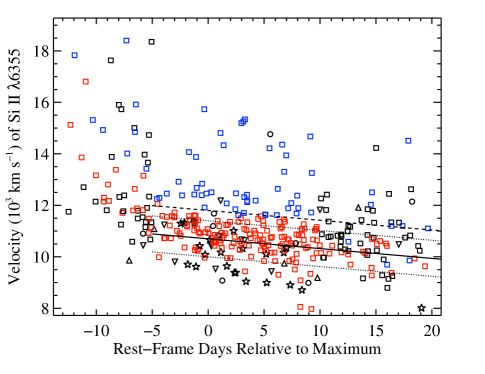
Figure 5: The velocity of Si ii $\lambda$6355 versus rest-frame age relative to maximum brightness of 360 spectra of 235 SNe. Colours and shapes of data points are the same as in Figure 4. The solid line is the mean evolution of the normal-velocity SNe with $t>-5$ d, the dotted lines are the standard deviation of the normal-velocity objects within 5 d of maximum brightness, and the dashed line is the cutoff between HV and normal-velocity objects (only defined for spectra with $-5<t<10$ d). If there are multiple spectra for a given object, the spectrum closest to maximum brightness is used to determined whether it is normal velocity or HV. Thus, there can be blue squares that fall below the dashed line. Uncertainties in the velocities are smaller than the size of the data points.

5.1.3 S ii

The temporal evolution of the S ii “W” velocity (calculated using the minimum of the redder of the two absorption features relative to its rest wavelength) is shown in the bottom left of Figure 4 and is quite linear from about 10 d before maximum brightness through 10 d after maximum. At about 5 d before maximum the typical velocity is $\sim\!\!$ 10,000 km s^-1, and by 5 d after maximum the typical velocity is $\sim\!\!$ 8000 km s^-1. As expected, the HV objects have larger velocities on average than the normal objects, but again there is significant overlap between the two subclasses. In addition, it seems that some of the HV objects decrease in velocity more quickly than the normal objects such that they have about the same velocity as the Ia-norm at the time of maximum brightness (see Section 5.2 for more information regarding the change of velocities with time). The Ia-91T/99aa objects have relatively large velocities for the S ii “W” feature, similar to the HV SNe. Like the velocities of the Si ii $\lambda$6355 feature, the Ia-91bg objects have many of the lowest velocities measured in this work (where we have excluded some of the slowest expanding, most peculiar SNe Ia).

5.1.4 O i

The O i triplet (Figure 4, bottom right) behaves in a manner similar to that of the Ca ii features. The velocities remain constant in most of our spectra. However, the typical post-maximum velocity, $\sim\!\!$ 11,000 km s^-1, is lower than that of the Ca ii features and has less scatter. The cluster of 6 spectra at extremely low velocities all have relatively weak O i triplets, and since this feature is so broad, determining the exact minimum when it is weak can be somewhat inaccurate. That being said, the visual checks of these fits reveal that they should be considered “good” fits. Like the Si ii $\lambda$6355 feature, most of the spectroscopically peculiar objects from all subclasses (Ia-91bg, Ia-91T, and Ia-99aa) have lower than average velocities, although there is much scatter in the velocities of the Ia-91bg SNe.

5.1.5 Summary of Velocity Evolution

Within a few days of maximum brightness, the typical velocities of the Ca ii features are 12,000–15,000 km s^-1, those of the Si ii and O i features are 10,000-11,000 km s^-1, and that of the S ii feature is $\sim\!\!$ 9000 km s^-1. These differences in velocities support the idea of the layered structure of SN Ia ejecta, with Ca ii found predominantly in the outermost (i.e., fastest expanding) layers, and O i, Si ii, and S ii found mainly in the inner (i.e., slower expanding) layers. Ca ii shows the largest velocity scatter and is likely well mixed from the outermost layers into moderately deeper layers of the ejecta. O i, Si ii, and S ii all show velocity scatter similar to each other (and smaller than that of Ca ii), implying that they are probably not as thoroughly mixed throughout the ejecta.

When comparing the velocities of most of the features investigated here, the typical near-maximum velocity of the normal SNe is in fact lower than that of the HV objects. However, this difference in velocities is relatively small in most cases, and there is significant overlap in the velocities spanned by the normal and HV SNe. By construction, the normal and HV objects have significantly different Si ii $\lambda$6355 velocities, but even in the other Si ii features there is a fair amount of overlap among the two subclasses. Furthermore, in Figure 5, there does not appear to be a strong distinction between the normal and HV objects, and thus a sharp cut to define these subclasses does not seem very well motivated.

Ia-91bg objects tend to have expansion velocities lower than those of spectroscopically normal SNe, with the Si ii $\lambda$6355 velocities being the most extreme case, though there is much overlap among the velocities for these subclasses. Ia-91T/99aa objects, on the other hand, are much more complicated. While there is significant scatter in the velocities calculated for these SNe, they are sometimes found to have higher than average velocities (in the Ca ii and S ii features) and sometimes smaller than average velocities (in the Si ii $\lambda$6355 and O i features).

Even though we question the idea of two distinct velocity populations of spectroscopically normal SNe Ia, it has been shown that normal and HV objects may have different intrinsic reddening or colours (Wang et al., 2009; Foley & Kasen, 2011). The BSNIP data seem to indicate, however, that instead of two distinct populations with two different intrinsic colours, there is likely a (nearly) continuous distribution of near-maximum velocities which may be correlated with intrinsic colour (or reddening). This is supported by recent theoretical models and interpretations of these models that explain the existence of normal and HV SNe Ia based on different viewing angles to the SNe (Kasen & Plewa, 2007; Kasen et al., 2009; Maeda et al., 2010; Foley & Kasen, 2011; Foley et al., 2011). Further investigations into these models and the photometric differences between HV and normal-velocity objects will be conducted in future BSNIP studies.

5.2 Velocity Gradients

One way to quantify how expansion velocities of SNe Ia evolve with time is to calculate their velocity gradient. Benetti et al. (2005) defined the velocity gradient, $\dot{v}=-\Delta v/\Delta t$, as the “average daily rate of decrease of the expansion velocity” of the Si ii $\lambda$6355 feature. Note that the BSNIP sample is not the best suited for this kind of study since the average number of spectra per object is relatively low ($\sim\!\!$ 2; Silverman et al., 2012). Therefore, the majority of the objects in our dataset have only a single near-maximum spectrum and we do not attempt to determine a velocity gradient for these objects. Despite this limitation, there are still quite a few SNe with multiple spectra in the sample analysed here for which we can calculate a velocity gradient.

While previous studies have mainly used only post-maximum velocities, for our $\dot{v}$ calculations we utilise velocities from spectra with $t\geq-5$ d. This is reasonable since, as can be seen in Figure 5, the velocities of the Si ii $\lambda$6355 feature decay linearly starting at $t\approx-5$ d, and this allows us to add more SNe to our $\dot{v}$ investigation. The velocity gradient is calculated using a linear least-squares fit to all the velocities of a given SN Ia measured from spectra with $-5\leq t\leq 20$ d; the uncertainty in $\dot{v}$ is computed from this linear fit.

Using the velocity gradient, Benetti et al. (2005) found that their sample of 26 SNe Ia could be divided into three subclasses. The high velocity gradient (HVG) group had the largest velocity gradients ($\dot{v}\ga 70$ km s^-1 d^-1) and consisted of Ia-norm, while the low velocity gradient (LVG) group had the smallest velocity gradients and included Ia-norm as well as Ia-91T/99aa. The third subclass (FAINT) had the lowest expansion velocities, yet moderately large velocity gradients, and consisted of subluminous SNe Ia (i.e., Ia-91bg) with $\Delta m_{15}(B)\ga 1.6$ mag. The same subclasses and criteria for membership are used in the study presented here. Note that the largest velocity gradient presented by Benetti et al. (2005) or Hachinger et al. (2006) is 125 km s^-1 d^-1, while the BSNIP data contain 12 SNe with $\dot{v}\ga 200$ km s^-1 d^-1.

Despite the fact that the BSNIP dataset only averages about two spectra per object, a velocity gradient can be calculated for 61 of the SNe Ia. The computed values of $\dot{v}$ (and their uncertainties), along with the photometric references which are the sources of the $\Delta m_{15}$ values used to determine whether or not a SN is FAINT, are presented in Table 3. The classification (i.e., Type) of each of these objects is also shown in Table 3 as well as in the “Benetti Type” column of Table LABEL:t:data.

Table 3: Velocity Gradients and Interpolated/Extrapolated Velocities

SN Name	Type${}^{\textrm{a}}$	LC Ref.${}^{\textrm{b}}$	$\dot{v}$${}^{\textrm{c}}$	$v_{0}$${}^{\textrm{d}}$	$v_{10}$${}^{\textrm{d}}$
SN 1989M	HVG	Ganeshalingam et al. (2010)	291.84 (139.49)	13.19 (0.42)	10.27 (0.98)
SN 1991bg†	FAINT	Hicken et al. (2009)	131.31 (6.44)	10.50 (0.07)	9.19 (0.10)
SN 1994D†	LVG	Hicken et al. (2009)	33.43 (6.77)	10.60 (0.06)	10.27 (0.09)
SN 1999ac	HVG	Ganeshalingam et al. (2010)	445.41 (49.10)	9.90 (0.13)	5.45 (0.61)
SN 1999cp	LVG	Ganeshalingam et al. (2010)	32.36 (15.43)	10.65 (0.16)	10.32 (0.07)
SN 1999da	FAINT	Ganeshalingam et al. (2010)	131.17 (15.56)	11.05 (0.08)	9.73 (0.14)
SN 1999dq	HVG	Ganeshalingam et al. (2010)	83.64 (20.04)	10.92 (0.07)	10.08 (0.22)
SN 1999gh†	FAINT	Jha et al. (2006)	46.49 (10.13)	11.21 (0.13)	10.74 (0.17)
SN 2000dk	FAINT	Ganeshalingam et al. (2010)	108.19 (14.04)	11.30 (0.11)	10.21 (0.09)
SN 2000dm	HVG	Ganeshalingam et al. (2010)	97.14 (14.08)	11.28 (0.08)	10.31 (0.12)
SN 2000dn	LVG	Ganeshalingam et al. (2010)	49.24 (7.95)	10.18 (0.09)	9.69 (0.07)
SN 2001bg	HVG*	Ganeshalingam et al. (2010)	228.90 (26.52)	14.56 (0.44)	12.27 (0.18)
SN 2001da	HVG	Ganeshalingam et al. (2010)	88.17 (12.75)	11.50 (0.09)	10.62 (0.10)
SN 2001en	HVG	Ganeshalingam et al. (2010)	103.48 (29.98)	13.31 (0.38)	12.28 (0.10)
SN 2001ep†	HVG	Ganeshalingam et al. (2010)	96.18 (26.92)	10.45 (0.15)	9.49 (0.31)
SN 2002bo	HVG	Ganeshalingam et al. (2010)	245.14 (8.12)	13.61 (0.09)	11.16 (0.07)
SN 2002cd	LVG	Ganeshalingam et al. (2010)	17.91 (8.33)	14.83 (0.11)	14.65 (0.07)
SN 2002de	HVG	Ganeshalingam et al. (2010)	96.88 (15.94)	11.89 (0.09)	10.92 (0.12)
SN 2002eu	HVG?	$\cdots$	119.97 (14.63)	11.07 (0.10)	9.87 (0.10)
SN 2002ha†	LVG	Ganeshalingam et al. (2010)	15.54 (15.55)	10.90 (0.08)	10.74 (0.18)
SN 2002hd	HVG*	Ganeshalingam et al. (2010)	116.29 (22.08)	11.17 (0.22)	10.01 (0.07)
SN 2002he†	HVG	Ganeshalingam et al. (2010)	81.01 (31.94)	12.57 (0.06)	11.76 (0.33)
SN 2003he	LVG	Ganeshalingam et al. (2010)	14.49 (23.71)	11.39 (0.15)	11.25 (0.12)
SN 2003iv	HVG?	$\cdots$	98.60 (28.67)	11.42 (0.14)	10.43 (0.18)
SN 2004bl	HVG?	$\cdots$	70.91 (9.33)	11.01 (0.13)	10.30 (0.07)
SN 2004dt	HVG	Ganeshalingam et al. (2010)	269.45 (8.34)	14.71 (0.11)	12.01 (0.07)
SN 2004fu	HVG?	$\cdots$	211.06 (27.37)	12.36 (0.07)	10.25 (0.29)
SN 2005M	HVG	Ganeshalingam et al. (2010)	86.36 (137.62)	8.77 (1.20)	7.90 (0.19)
SN 2005am	FAINT	Ganeshalingam et al. (2010)	61.11 (72.62)	11.74 (0.40)	11.13 (0.34)
SN 2005bc	LVG	Ganeshalingam et al. (2010)	64.63 (23.70)	11.01 (0.13)	10.37 (0.15)
SN 2005cf	HVG	Ganeshalingam et al. (2010)	106.69 (149.59)	10.14 (0.26)	9.07 (1.74)
SN 2005de	HVG	Ganeshalingam et al. (2010)	70.45 (12.73)	10.86 (0.09)	10.15 (0.10)
SN 2005el	LVG	Ganeshalingam et al. (2010)	13.46 (20.10)	10.95 (0.12)	10.81 (0.13)
SN 2005er	HVG?	$\cdots$	228.72 (71.21)	10.02 (0.09)	7.73 (0.67)
SN 2005eq	HVG	Ganeshalingam et al. (2010)	76.47 (37.84)	9.58 (0.08)	8.82 (0.43)
SN 2005ki	LVG	Ganeshalingam et al. (2010)	24.19 (20.54)	11.27 (0.12)	11.03 (0.12)
SN 2005ms	HVG	Hicken et al. (2009)	115.00 (8.36)	10.95 (0.09)	9.80 (0.08)
SN 2005na	HVG	Ganeshalingam et al. (2010)	288.79 (138.17)	10.93 (0.10)	8.04 (1.31)
SN 2006N†	HVG	Hicken et al. (2009)	84.84 (8.96)	11.20 (0.06)	10.35 (0.11)
SN 2006S†	LVG	Hicken et al. (2009)	35.46 (6.02)	10.60 (0.07)	10.25 (0.09)
SN 2006bq†	HVG*	Ganeshalingam et al. (2010)	219.70 (15.82)	15.47 (0.20)	13.27 (0.25)
SN 2006bt	HVG	Ganeshalingam et al. (2010)	223.70 (20.34)	11.04 (0.07)	8.80 (0.24)
SN 2006dm	HVG	Ganeshalingam et al. (2010)	131.21 (23.46)	11.49 (0.28)	10.18 (0.08)
SN 2006ej	HVG	Ganeshalingam et al. (2010)	92.24 (15.78)	12.11 (0.07)	11.19 (0.16)
SN 2006eu	HVG	Ganeshalingam et al. (2010)	356.38 (23.54)	14.50 (0.32)	10.94 (0.10)
SN 2006et	LVG	Ganeshalingam et al. (2010)	16.07 (23.52)	9.49 (0.16)	9.32 (0.11)
SN 2006ev	HVG?	$\cdots$	82.46 (23.77)	12.69 (0.33)	11.86 (0.11)
SN 2006ke	HVG?	$\cdots$	111.91 (22.80)	9.65 (0.14)	8.53 (0.13)
SN 2006sr	HVG	Hicken et al. (2009)	152.37 (27.60)	12.03 (0.07)	10.51 (0.28)
SN 2007A	LVG?	$\cdots$	22.10 (10.87)	10.83 (0.12)	10.61 (0.07)
SN 2007af†	HVG	Ganeshalingam et al. (2010)	72.01 (25.73)	10.91 (0.07)	10.19 (0.27)
SN 2007co†	LVG	Ganeshalingam et al. (2010)	41.96 (10.01)	11.43 (0.06)	11.01 (0.12)
SN 2007fb	LVG?	$\cdots$	52.78 (10.90)	11.46 (0.11)	10.93 (0.07)
SN 2007gi	HVG?	$\cdots$	197.68 (20.12)	15.66 (0.09)	13.69 (0.15)
SN 2007gk	HVG?	$\cdots$	138.74 (6.50)	13.83 (0.09)	12.44 (0.07)
SN 2007hj	FAINT	Ganeshalingam et al. (2010)	133.27 (10.06)	12.26 (0.09)	10.92 (0.08)
SN 2007le†	HVG	Ganeshalingam et al. (2010)	93.35 (12.65)	12.78 (0.18)	11.84 (0.22)
SN 2008dx	FAINT*	Ganeshalingam et al. (2010)	97.91 (28.21)	9.62 (0.15)	8.64 (0.16)
SN 2008ec†	LVG	Ganeshalingam et al. (2010)	68.61 (10.82)	11.01 (0.09)	10.33 (0.14)
SN 2008ei	HVG*	Ganeshalingam et al. (2010)	114.40 (23.97)	15.72 (0.16)	14.57 (0.11)
SN 2008s5${}^{\textrm{e}}$	LVG*	Ganeshalingam et al. (2010)	11.86 (17.85)	9.09 (0.11)	8.97 (0.11)
Uncertainties are given in parentheses.
†This object has more than two near-maximum spectra that were used to calculate $\dot{v}$.
${}^{\textrm{a}}$Classification based on the velocity gradient of the Si II $\lambda$6355 line (Benetti et al., 2005). “HVG” = high velocity gradient; “LVG” = low velocity gradient; “FAINT” = faint/underluminous. Classifications marked with a “?” are uncertain since light-curve shape information is unavailable. Classifications marked with a “*” use the MLCS2k2 $\Delta$ parameter (Jha et al., 2007) as a proxy for $\Delta m_{15}$.
${}^{\textrm{b}}$Source of $\Delta m_{15}$ (or MLCS2k2 $\Delta$) value.
${}^{\textrm{c}}$The velocity gradient is in units of km s-1 day-1.
${}^{\textrm{d}}$The velocity is calculated from the Si II $\lambda$6355 line and is in units of 1000 km s-1.
${}^{\textrm{e}}$Also known as SNF20080909-030.

The 11 objects in Table 3 that have classifications marked with a “?” are uncertain since light-curve shape information is unavailable, so their classification is based only on their velocity gradient. As we will show below, FAINT objects have similar $\dot{v}$ values to HVG objects, thus some of the HVG? could in fact be part of the FAINT subclass. The 6 SNe in Table 3 that have classifications marked with a ‘*’ use the MLCS2k2 $\Delta$ parameter (Jha et al., 2007) as a proxy for $\Delta m_{15}$.

Most LVG and FAINT objects are also normal velocity (as opposed to HV) objects and have the lowest velocities observed (specifically in the Si ii and Ca ii features). This confirms what was observed by Benetti et al. (2005). The HVG subclass contains both normal and HV objects. Many HVG objects have relatively high velocities at early times, but then evolve to have normal to somewhat low velocities by about 10 d past maximum brightness. This confirms what was seen in at least one previous study (Pignata et al., 2008), but differs from what has been seen (and assumed) in other previous work (Benetti et al., 2005; Wang et al., 2009; Foley & Kasen, 2011). In the latter studies, HVG objects were claimed to have higher velocities than LVG and FAINT objects from before maximum through $t\approx 10$ d. While most HVG BSNIP SNe start out at high velocities before and near maximum brightness, our data are in agreement with Pignata et al. (2008) and show that they evolve to average (or even relatively low) velocities by only a few days after maximum.

These observations can be explained using the off-centre explosion models of Maeda et al. (2010). In their models, different viewing angles will result in a wide range of observed velocities and velocity gradients. The models also indicate that before maximum brightness, the highest velocity objects have the largest velocity gradients, but the velocities of all of their models become quite similar by 10 d after maximum, much like what is observed in our data.

In Table 4 we present the averages and standard deviations of $\Delta m_{15}$ and $\dot{v}$ for each subclass (with and without SNe having uncertain classifications due to a lack of photometric data), as well as the number of SNe in each subclass. HVG is the largest group and only a few SNe fall into the FAINT subclass. Comparing these numbers to those of Benetti et al. (2005), we find a similar number of LVG and FAINT objects, but significantly more HVG SNe. These differences are interesting to note, but may not have any physical significance since the sample used by Benetti et al. (2005) contained only well-observed SNe Ia which perhaps biased the sample to contain more peculiar or bright or nearby objects since these have historically been better observed. They also used spectra from a variety of sources which could introduce systematic biases into their analysis, and they measure velocities from their first epoch until the last epoch in which the Si ii $\lambda$6355 feature is detected. The BSNIP dataset used here contains spectra of all subtypes of SNe Ia (in roughly the same proportions as what was analysed in Ganeshalingam et al., 2010) having $t<20$ d and obtained using a small number of instruments and reduced by only a few people (see BSNIP I for more on the homogeneity of the BSNIP dataset).

Table 4: Summary of Velocity Gradient Subtypes

Type	$\Delta m_{15}$ (mag)	$\dot{v}$ (km s-1 d-1)	$v_{0}$ ($10^{3}$ km s-1)	$v_{10}$ ($10^{3}$ km s-1)	# of Objects
LVG	1.16 (0.24)	31.37 (18.91)	10.96 (1.30)	10.64 (1.32)	14
LVG + LVG?	$\cdots$	32.13 (18.59)	10.98 (1.22)	10.66 (1.23)	16
HVG	1.22 (0.22)	156.12 (98.23)	11.98 (1.78)	10.42 (1.75)	29
HVG + HVG?	$\cdots$	152.30 (89.92)	11.98 (1.78)	10.46 (1.75)	38
FAINT	1.80 (0.13)	101.35 (35.34)	11.10 (0.85)	10.08 (0.93)	07
Average values are shown and standard deviations are given in parentheses.
Average $\Delta m_{15}$ values are undefined for the rows that include objects with no light-curve shape information.
Note that the average $\Delta m_{15}$ values do not include the 6 objects that use $\Delta$ as a proxy for $\Delta m_{15}$.

The average $\Delta m_{15}$ is about the same for all of the subclasses except FAINT. This is partially by construction since all SNe with $\Delta m_{15}>1.6$ mag are considered FAINT. However, the fact that LVG and HVG objects all have effectively the same average $\Delta m_{15}$ value implies that $\dot{v}$ and $\Delta m_{15}$ are not correlated. This has been seen before, and previous similar studies found nearly identical average $\Delta m_{15}$ values for each subclass (e.g., Benetti et al., 2005).

By construction, the velocity gradients of LVG objects are significantly lower than those of HVG objects. Perhaps somewhat surprisingly, HVG and FAINT SNe have similar values of $\dot{v}$. The average value of $\dot{v}$ for each subclass is effectively unchanged when objects with uncertain classifications are included, implying that the LVG? objects are almost certainly all bona fide LVG SNe. However, it is unclear whether the HVG? are truly HVG or if they are actually part of the FAINT subclass. While the average $\dot{v}$ for the LVG and HVG objects is nearly equal to those from Benetti et al. (2005), the average velocity gradient for the FAINT SNe is somewhat larger in our sample (although they are within one standard deviation of each other). Also, the average velocity gradient of the HVG objects is larger than that of Benetti et al. (2005), due to the handful of SNe with significantly larger $\dot{v}$ values than what has been seen previously.

As stated earlier, the BSNIP sample is not the best suited for this kind of study since the average number of spectra per object is relatively low. If we restrict ourselves to only objects with more than two near-maximum spectra (i.e., SNe marked with a “^†” in Table 3), we are left with 6 HVG objects, 5 LVG objects, and 2 FAINT objects (which used $\Delta$ as a proxy for $\Delta m_{15}$). One might worry, based on these numbers, that many of our HVG objects are a result of the large uncertainty introduced when calculating the velocity gradient using only two data points. However, the average $\Delta m_{15}$ and $\dot{v}$ for each subclass is consistent with that of the entire sample when only using objects with more than two spectra. It should be noted that the average velocity gradient for the HVG subclass does decrease when applying this cut and actually becomes smaller than the one calculated by Benetti et al. (2005). Similarly, the FAINT subclass’ average $\dot{v}$ becomes approximately equal to the one in Benetti et al. (2005) when only using SNe with more than two spectra. One caveat is that the fact that there are more than two spectra of these objects in the BSNIP dataset may imply that they are particularly interesting objects that are peculiar, intrinsically bright, nearby, or well separated from their host galaxy. While these may be true and could lead to a bias in this subsample, all of these objects are Ia-norm except for one Ia-91bg and one Ia-99aa.

5.3 Interpolated/Extrapolated Velocities

Once a velocity gradient is calculated for a SN Ia, one can interpolate/extrapolate that gradient to determine the expansion velocity at a specified epoch. Benetti et al. (2005) defined $v_{10}$ as the expansion velocity of Si ii $\lambda$6355 at 10 d past maximum brightness. Similarly, Hachinger et al. (2006) interpolate/extrapolate their expansion velocities to the time of maximum brightness (i.e., $t=0$ d), and so $v_{0}$ is defined here as the expansion velocity of Si ii $\lambda$6355 at maximum brightness. For each SN where $\dot{v}$ is calculated, $v_{0}$ and $v_{10}$ are also calculated. The uncertainties of these two velocities are computed by propagating the uncertainties in the linear fit (when more than two spectra are used) or, when only two spectra are used to determine the velocity gradient, by propagating the uncertainties in the two velocity measurements themselves. The computed values of $v_{0}$ and $v_{10}$ (and their uncertainties) are presented in Table 3, and the averages and standard deviations of these velocities for each subclass are displayed in Table 4.

This interpolation/extrapolation calculation allows a more self-consistent comparison of the expansion velocities of different objects. By the simple fact that we calculate nonzero velocity gradients, the expansion velocities are changing with time and not all of our objects were observed at exactly the same epochs. This procedure also enables us to make more quantitative statements regarding the differences in expansion velocities among various subclasses of SNe Ia.

As expected, at maximum brightness all objects determined to be HV do in fact have $v_{0}>11,800$ km s^-1 and the opposite is true for objects determined to have normal velocities. This can be seen in the top panel of Figure 6, where we plot $v_{0}$ versus $\dot{v}$ for all SNe having a measured velocity gradient. All blue points (HV SNe) are to the right of the vertical line at $v_{0}=11,800$ km s^-1 and all red points (normal velocity SNe) are to the left of it. This sanity check is encouraging and implies that our HV determination (as outlined in Section 5.1) is relatively robust at maximum brightness.

$\begin{array}[]{c}\includegraphics[width=252.94499pt]{v0_v_dot}\\ \includegraphics[width=252.94499pt]{v10_v_dot}\end{array}$

Figure 6: $v_{0}$ versus $\dot{v}$ (top) and $v_{10}$ versus $\dot{v}$ (bottom) for all SNe where we calculate a velocity gradient. Blue points are HV objects, red points are normal-velocity objects, and black points are objects for which we could not determine whether the SN was normal or high velocity. Squares are low velocity gradient (LVG) objects, circles are possible LVG objects, stars are FAINT objects, upward-pointing triangles are high velocity gradient (HVG) objects, and downward-pointing triangles are possible HVG objects. The vertical dashed line in the top panel is our HV cutoff ($v_{0}=11,800$ km s^-1). The solid line is a linear fit to the “moderate decliners” ($1<\Delta m_{15}<1.5$ mag, whose data points are circled). The vertical dashed line in the bottom panel is our HV cutoff at $t=0$ d (11,800 km s^-1) decreased by the average velocity gradient for the normal-velocity SNe (38 km s^-1 d^-1) for 10 d (i.e., $v_{10}=11,420$ km s^-1$=11,800-10\times 38$). The slanted dotted line in the bottom panel is our HV cutoff at $t=10$ d as a function of $\dot{v}$ (i.e., $v_{10}=11,800-10\times\dot{v}$).

While there does not appear to be a strong correlation between $\dot{v}$ and $v_{0}$, it does at least seem that, on average, objects with larger velocity gradients tend to have larger velocities at maximum light, though there are plenty of SNe Ia that do not follow this correlation. The average $v_{0}$ for LVG and FAINT SNe are approximately equal, while they are both lower than the average $v_{0}$ for HVG SNe (see the fourth column of Table 4).

The solid line in Figure 6 is a linear least-squares fit to the “moderate decliners” (i.e., $1<\Delta m_{15}<1.5$ mag, whose data points are circled in the Figure) of the form

$$\dot{v}=\alpha v_{0}+\beta.$$ (2)

We calculate $\alpha=55.0\pm 1.8$ and $\beta=-539\pm 22$ for $v_{0}$ in units of $10^{3}$ km s^-1 and $\dot{v}$ in units of km s^-1 d^-1. Foley et al. (2011) fit a similar relationship to their data in order to derive a family of functions. This allows them to calculate a velocity of the Si ii $\lambda$6355 feature at maximum brightness given a spectral age and a velocity at that age. They find $\alpha=32.2$ and $\beta=-285$, which are both significantly different than what is calculated for the BSNIP data. The large amount of scatter around the solid line in Figure 6 casts doubt on how useful the family of functions proposed by Foley et al. (2011) can actually be in calculating velocities at maximum brightness.

Somewhat surprising, however, is the wide range of $v_{0}$ values spanned by each of the subclasses. Even at maximum brightness, where the difference between HV and normal objects is defined, a HVG SN may have normal (or even relatively low) velocity. This is contrary to many previous studies that often assume a one-to-one correlation between HV and HVG and, similarly, between normal velocities and LVG (e.g., Hachinger et al., 2006; Pignata et al., 2008; Wang et al., 2009). Kolmogorov-Smirnov tests were performed on the $v_{0}$ values of LVG and HVG SNe (both including and excluding objects with uncertain classifications), and we find that they likely come from different parent populations ($p\approx 0.03$). Thus, it is still reasonable to associate LVG SNe with normal velocities at maximum and HVG SNe with HV objects, but we caution that this may not be as robust an association as was previously thought.

The connection between HVG and HV is even more tenuous by 10 d after maximum brightness. In the bottom panel of Figure 6 we plot $v_{10}$ versus $\dot{v}$ for all SNe where we calculate a velocity gradient. The vertical line is our HV cutoff value at $t=0$ d (11,800 km s^-1) decreased by the average velocity gradient for the normal-velocity SNe (38 km s^-1 d^-1) for 10 d (i.e., $v_{10}=11,420$ km s^-1$=11,800-10\times 38$). Naively, if one measured $v_{10}\la 11,420$ km s^-1 for a given SN, they might classify it as a normal-velocity object. However, about half of our HV SNe fall in this regime. This is actually expected since our HV definition only included velocities within 5 d of maximum, so extrapolating this analysis to 10 d past maximum may not be valid. If we instead plot our HV cutoff at $t=10$ d as a function of $\dot{v}$ (i.e., $v_{10}=11,800-10\times\dot{v}$), then we get the slanted line in the bottom panel of Figure 6. Now, the HV SNe all fall above this line while the normal-velocity objects are all below it. Effectively, some of the HVG objects have decreased their velocity fast enough to “catch up” with the velocities of the normal-velocity objects by this epoch. By 10 d past maximum brightness, a single velocity measurement alone is not sufficient to determine whether an object should be considered HV or not.

All three velocity gradient subclasses span nearly the full range of $v_{10}$ values and the average $v_{10}$ is effectively the same for all subclasses (see the fifth column of Table 4). Kolmogorov-Smirnov tests were performed on the $v_{10}$ values of LVG and HVG (both including and excluding objects with uncertain classifications), and we find no evidence that they come from different parent populations. Thus, by 10 d past maximum brightness the distributions of expansion velocities among LVG and HVG objects are consistent with each other.

As mentioned in Section 5.2, the off-centre explosion models of Maeda et al. (2010) may naturally explain the existence of HVG SNe. They also show that models with the largest velocity gradients have the highest velocities near maximum brightness, but by about 10 d after maximum the expansion velocities of almost all of their models become quite similar (independent of initial velocities or velocity gradients). These models seem to have observational grounding in the data we present here. Further comparisons to the models and predictions of Maeda et al. (2010), especially at later epochs, will be made in future BSNIP papers. Also, the velocity gradients, classifications, and interpolated/extrapolated velocities discussed here will be compared to photometric properties (such as light-curve shape and decline rate) in BSNIP III.

5.4 Temporal Evolution of Pseudo-Equivalent Widths

As with expansion velocities of SNe Ia, much work has been done previously on studying the pseudo-equivalent widths of various spectral features as they change with time (e.g., Folatelli, 2004; Garavini et al., 2007; Bronder et al., 2008; Walker et al., 2011; Nordin et al., 2011b; Konishi et al., 2011). The temporal evolution of the pEW for each of the nine spectral features is shown in Figure 7 and Figure 8. The “SNID type” is displayed rather than the “Benetti type” (see Section 5.2) in the pEW figures because the velocity gradient of an object does not appear to be well correlated with its pEW measurements.

Also shown in Figure 7 and Figure 8 are fits to the pEW evolution for each spectral feature (solid line) along with the RMSE of the fit (grey region), using only Ia-norm (with normal velocities). The parameters for each of the fits can be found in Table 5. For features whose pEW appears to evolve linearly with time a linear function is fit to the data, while features whose pEW have a sharp change in their temporal evolution have a quadratic function fit to them. This differs from previous studies which have modeled the behaviour of pEWs with time either using cubic splines (e.g., Garavini et al., 2007) or logistic functions instead of quadratic ones (Nordin et al., 2011b). As seen in the figures, the pEW temporal evolution for each spectral feature can be fit relatively well with either a linear or quadratic function. Experiments with fitting the pEW evolution with cubic splines and logistic functions were carried out, but the fits were either worse or comparable to those of the linear and quadratic functions (which have fewer free parameters).

Table 5: Fits to the pEW Temporal Evolution

Feature	Fit to pEW$\left(t\right)$
Ca ii H&K	115	$-$	$3.11t$	$+$	$0.0962t^{2}$
Si ii $\lambda$4000	18.5	$+$	$0.359t$
Mg ii	90.0	$+$	$0.679t$
Fe ii	135	$+$	$5.85t$	$+$	$0.254t^{2}$
S ii “W”	78.3	$-$	$0.0427t$	$-$	$0.332t^{2}$
Si ii $\lambda$5972	24.8	$+$	$0.454t$
Si ii $\lambda$6355	110	$+$	$1.29t$
O i triplet	110	$+$	$2.61t$	$-$	$0.354t^{2}$
Ca ii near-IR triplet	200	$+$	$7.62t$

Following Nordin et al. (2011b), we use our fits of the temporal evolution of the pEW for each spectral feature to attempt to “remove” the age dependence of the pEW. To do this, an epoch-independent quantity called the “pEW difference” ($\Delta$pEW) is defined; it is simply the measured pEW minus the expected pEW at the same epoch using the linear or quadratic fit. The uncertainty in $\Delta$pEW comes from combining the uncertainty of the pEW measurement with the RMSE of the fit. The $\Delta$pEW values and their uncertainties can be found in Tables B1–B9. Note that while the fits were defined using only Ia-norm, $\Delta$pEW values are calculated for SNe of all spectral types.

5.4.1 Ca ii

The Ca ii H&K feature and the Ca ii near-IR triplet show a cluster of spectra with relatively large pEW at $t<-5$ d in Figure 7 (top row). This is perhaps due to detached, high-velocity absorption blending with the normal-velocity component (e.g., Branch et al., 2005). For $t\ga-5$ d, the pEW of the Ca ii H&K feature decreases slightly and the scatter in the pEW values decreases markedly near $t\ga 10$ d. This feature is fit with a quadratic in order to encompass the relatively large number of objects with high pEW values at the earliest times as well as the decrease and eventual flattening out at later times. It is interesting to note that the typical pEW for the HV objects is larger than that of the normal-velocity objects (for $t\la 10$ d).

Despite the fact that there are not that many spectroscopically peculiar objects plotted in the top-left panel of Figure 7, it seems that Ia-91bg follow the evolution of the Ia-norm objects while Ia-91T/99aa are below the typical pEW values (and thus have negative values of $\Delta$pEW). This matches what has been observed previously in other low-redshift datasets (Garavini et al., 2007; Bronder et al., 2008).

On the other hand, the Ca ii near-IR triplet pEW values increase linearly with time after about 5 d before maximum (which is why the evolution of this feature is fit with a linear function). Also distinct from the Ca ii H&K feature, the typical pEW of the HV and normal objects is about the same. While the Ia-91T/99aa objects are certainly below the normal pEW values, the Ia-91bg objects have pEWs that are well above the normal evolution. Once again, this has been noted previously, though the few large pEW values at early times have not been seen and our sample has far more data points than earlier work (Folatelli, 2004).

$\begin{array}[]{cc}\includegraphics[width=252.94499pt]{ew_t_cahk}&\includegraphics[width=252.94499pt]{ew_t_cair}\\ \includegraphics[width=252.94499pt]{ew_t_si6355}&\includegraphics[width=252.94499pt]{ew_t_si4000}\\ \includegraphics[width=252.94499pt]{ew_t_si5972}&\includegraphics[width=252.94499pt]{ew_t_mg}\\ \end{array}$

Figure 7: The pEW versus rest-frame age relative to maximum brightness for various spectral features: (top left) 281 spectra of 191 SNe for Ca ii H&K, (top right) 301 spectra of 201 SNe for the Ca ii near-IR triplet, (middle left) 366 spectra of 239 SNe for Si ii $\lambda$6355, (middle right) 188 spectra of 137 SNe for Si ii $\lambda$4000, (bottom left) 204 spectra of 156 SNe for the Si ii $\lambda$5972 feature, and (bottom right) 219 spectra of 163 SNe for the Mg ii complex. Colours and shapes of data points are the same as in Figure 4. The solid curve is a linear or quadratic fit to the data using only Ia-norm; the grey region is the RMSE of the fit.

$\begin{array}[]{cc}\includegraphics[width=252.94499pt]{ew_t_fe}&\includegraphics[width=252.94499pt]{ew_t_sw}\\ \includegraphics[width=252.94499pt]{ew_t_oi}&\\ \end{array}$

Figure 8: The pEW versus rest-frame age relative to maximum brightness for various spectral features: (top left) 313 spectra of 217 SNe for the Fe ii complex, (top right) 240 spectra of 179 SNe for the S ii “W” feature, and (bottom left) 192 spectra of 139 SNe for the O i triplet. Colours and shapes of data points are the same as in Figure 4. The solid curve is a linear or quadratic fit to the data using only Ia-norm; the grey region is the RMSE of the fit.

5.4.2 Si ii

The pEW of the Si ii $\lambda$6355 feature (Figure 7, middle left) linearly increases with time before $t\approx 10$ d and shows a hint of a sharp upturn thereafter (however, this is likely due to the feature becoming blended with Si ii $\lambda$5972 at these later epochs). Also, before $\sim\!\!$ 10 d past maximum the HV objects have a larger typical pEW than the normal-velocity objects. Like the Ca ii H&K feature, the Ia-91T/99aa objects fall well below the normal evolution while the Ia-91bg span a large range of pEW values (from well below to well above the average evolution). This behaviour is similar to that seen in the low-$z$ (and moderate-$z$) samples of Folatelli (2004) and Konishi et al. (2011).

The temporal evolution of the pEW of the Si ii $\lambda$4000 feature (Figure 7, middle right) is quite unique. There is evidence for two distinct evolutionary tracks: one rising until 2–3 d past maximum and then declining, and one constant (and lower) until 2–3 d past maximum and then rising. The two groups are effectively blended into one another by $\sim\!\!$ 5 d past maximum. This creates a gap at relatively low values of pEW from a few days before maximum until a few days after maximum. The two-component evolution has been seen in other datasets, but the gap in the present sample is not nearly as pronounced as in some of the earlier studies which used many fewer data points (Folatelli, 2004; Bronder et al., 2008). Out of 35 SNe Ia with multiple measurements of the pEW of Si ii $\lambda$4000, two objects transition from the higher track to the lower one while none transition the other direction.

There is no significant difference in pEW of the Si ii $\lambda$4000 feature between HV and normal-velocity objects, though almost all of the HV objects are found in the “upper evolutionary track.” While there are only a small number of Ia-91bg objects for which we measure a pEW for the Si ii $\lambda$4000 feature, they also fall well within the “upper evolutionary track.” The Ia-91T/99aa SNe are found only in the “lower evolutionary track.” Note that Ia-norm objects are found in both tracks.

The $\Delta$pEW values of the Si ii $\lambda$4000 have been found to correlate with SN colour as well as velocity gradient (Nordin et al., 2011a). In BSNIP III the relationship between both $\Delta$pEW and pEW and SN colour for this feature will be investigated. In Figure 9 we plot $\Delta$pEW of Si ii $\lambda$4000 against $-\dot{v}$ (the minus sign is used here in order to match the velocity gradient definition of Nordin et al., 2011a) for all objects with $0\leq t\leq 8$ d. Our plot contains 31 SNe Ia as compared to the 20 objects shown in Figure 3 of Nordin et al. (2011a), and we also follow their convention of taking the mean $\Delta$pEW value for objects with multiple spectra in the epoch range studied.

The basic trends seen in Figure 9 are unchanged if we use pEW instead of $\Delta$pEW, and are similar to what was observed by Nordin et al. (2011a). The biggest difference between the two studies is that Nordin et al. (2011a) use only spectroscopically normal SNe (thus they would not have the four black points at the bottom right of Figure 9), and they do not see the most extreme HVG objects which appear in our dataset (i.e., the two left-most points in Figure 9). Nordin et al. (2011a) claim a “strong correlation” between $\Delta$pEW values of Si ii $\lambda$4000 and velocity gradient (quoting a Spearman rank coefficient of $-0.73$). A fit to the BSNIP data (excluding the 6 aforementioned outlier objects which are ignored or not seen in their sample) yields a Spearman rank coefficient of $-0.54$, which implies that the supposed correlation may not actually be all that significant.

There is a relatively large scatter in the pEW values measured for the Si ii $\lambda$5972 feature (Figure 7, bottom left). Evidence suggests that the pEW values are trending slightly upward with time; however, this is driven mainly by points at $t\ga 5$ d where we might expect the Si ii $\lambda$5972 feature to start blending with the Na i D line, which can appear in SN Ia spectra near this epoch (e.g., Branch et al., 2005). Ignoring points at $t>5$ d, the temporal evolution is relatively constant, although the HV objects are perhaps decreasing slightly with time. Once again, the Ia-91T/99aa objects have relatively small pEW values while the Ia-91bg SNe lie well above the average evolution. This matches the trends seen in the low-$z$ data presented by Folatelli (2004) and Konishi et al. (2011).

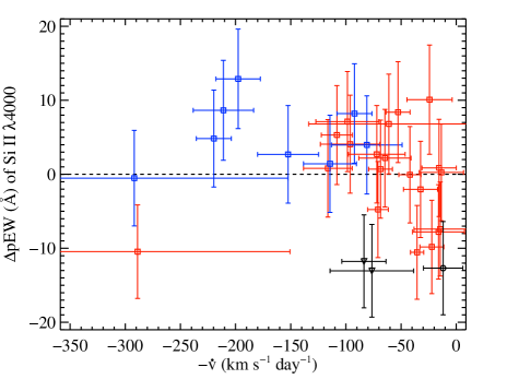
Figure 9: The $\Delta$pEW of Si ii $\lambda$4000 versus $-\dot{v}$ (the minus sign is used here in order to match the velocity-gradient definition of Nordin et al., 2011a) for all 31 objects with $0\leq t\leq 8$ d. Colours and shapes of data points are the same as in Figure 4.

5.4.3 Mg ii

The temporal evolution of the pEW of the Mg ii complex (Figure 7, bottom right) has relatively small scatter and linearly increases slightly with time. The HV objects have larger pEW values (and more scatter) than the normal-velocity objects. Interestingly, this evolution is markedly different from what has been seen in some other low-$z$ samples (Folatelli, 2004; Garavini et al., 2007). While the BSNIP data match these previous studies until $t\approx 10$ d, there is no evidence for the sudden increase in pEW values for this feature. In fact, no attempt is made to measure the pEW of the Mg ii complex beyond $t\approx 10$ d because it becomes too blended with the Si ii $\lambda$4000 feature (as pointed out by Garavini et al., 2007). Folatelli (2004) simply define a larger wavelength range at these epochs (see their Fig. 1, feature 3), which will certainly increase the measured pEW. Our temporal evolution does, however, match what was seen by Walker et al. (2011).

The Ia-91T/99aa objects are yet again found to have lower than average pEW values. On the other hand, the Ia-91bg objects have somewhat higher than average pEW values, but there are very few of these types of objects for which a pEW is successfully measured. This is due to the fact that when the Mg ii complex is strong before and near maximum brightness, as it often is for Ia-91bg SNe due to additional absorption from Ti ii (e.g., Bronder et al., 2008), it becomes severely blended with Si ii $\lambda$4000, and thus no attempt is made to measure its pEW. This is further supported by the fact that we see no objects with a pEW of Mg ii $\ga 140$ Å, while data in Garavini et al. (2007) and the low-$z$ sample presented by Bronder et al. (2008) contain several objects with such large pEW values.

5.4.4 Fe ii

While the Mg ii complex has a fairly tight linear pEW evolution, the pEW of the Fe ii complex (Figure 8, top left) shows an extremely tight temporal evolution which is almost certainly nonlinear (thus we fit it with a quadratic function). Another difference between these two features is that the Mg ii complex pEW values are nearly constant for $-10\la t\la 10$ d (increasing by $<20$ Å over that range) while the Fe ii complex pEWs increase dramatically during the same span of time ($\sim\!\!$ 130 Å). Despite these differences, the data for both the Mg ii and Fe ii complexes fall almost completely within the RMSE of their respective fits. Furthermore, the HV objects in both features have larger pEW values, as well as more scatter, than the normal-velocity objects.

As with the pEWs of the Mg ii feature, the Ia-91T/99aa objects are all below the fit to the Ia-norm. It is even more apparent for the Fe ii complex than it was for the Mg ii complex that the Ia-91bg objects are all found above the fit to the data. These differences, as well as the overall trends, have been recognised in numerous previous studies of both low-$z$ and moderate-$z$ SNe Ia (e.g., Folatelli, 2004; Garavini et al., 2007; Nordin et al., 2011b; Konishi et al., 2011).

5.4.5 S ii

The temporal evolution of the pEW values for the S ii “W” feature (Figure 8, top right) is unique. The pEW of the majority of objects increases until maximum brightness and then decreases in a nearly symmetric way. A quadratic function centred near $t=0$ d fits the data (especially the Ia-norm objects) very well. There is a possibility that the HV objects have higher pEW values before maximum (with equal pEW values after maximum), but the significance of this difference is relatively low. The Ia-91T/99aa objects have even lower pEW values than the normal-velocity objects before maximum, though they also seem to evolve to more average values after maximum brightness. The Ia-91bg objects, on the other hand, are almost all significantly below the average evolution at all epochs (though there are a few with relatively normal pEWs). The temporal evolution seen here confirms what was found by Nordin et al. (2011b) and Konishi et al. (2011) in their low-$z$ and moderate-$z$ data.

5.4.6 O i

The O i triplet’s average pEW values evolve in much the same way as those of the S ii “W,” with the normal pEW values rising until $\sim\!\!$ 4 d past maximum and then declining (Figure 8, bottom left). There is a hint that the HV objects might have smaller pEW values than the normal-velocity objects, though the scatter in both of these subclasses is quite large. As mentioned in Section 4.1.8, this feature is often strongly affected by telluric absorption, and thus some of the points which lie significantly away from the average evolution could be explained by imperfect telluric absorption corrections. This could also be the reason why we are able to measure pEWs of the O i triplet for relatively few Ia-91T/99aa objects. As was seen in the Ca ii features, the Ia-91T/99aa SNe have relatively low pEW values, and if their O i triplet pEWs are also small, then the feature could get “lost in the noise” after an inaccurate telluric absorption correction. The Ia-91bg objects, however, have large pEW values for $t\la 2$ d, but quickly decrease to more average values at later epochs.

5.4.7 Summary of pEW Evolution

As mentioned above, we chose to present the “SNID type” rather than the “Benetti type” in the pEW versus time figures because the velocity gradient of an object is not well correlated with any pEW measurements. The one species with a possible correlation is Si ii. In all three of its features, while the LVG and HVG objects show very little difference in pEW values, there is an indication that the pEWs of the FAINT objects are larger than the average values at each epoch. This is unsurprising since the Ia-91bg objects also have larger-than-average pEW values for the Si ii $\lambda$4000 and Si ii $\lambda$5972 features, and these SNe are also often underluminous (which is exactly how the FAINT subclass is defined).

When comparing the pEW values of normal and HV objects, for most of the features investigated here the typical pEWs of the HV SNe are larger than those of the normal-velocity objects. The HV SNe also tend to have more scatter in their pEW values. These two points are most noticeable in the Ca ii H&K, Mg ii, Fe ii, and Si ii $\lambda$6355 features. However, some of the features do show very similar pEW values between HV and normal-velocity objects, and the O i triplet’s typical pEW for HV SNe is perhaps smaller than that of normal-velocity objects. By $t\approx 10$ d the average pEW values of HV and normal-velocity SNe are nearly equal in almost all of the spectral features measured.

The velocity of the Si ii $\lambda$6355 feature is used to differentiate between HV and normal objects, so it may be unsurprising that the pEW of this same feature shows a marked split between these two subclasses. Somewhat more interesting is the fact that the other three features which exhibit a strong split in pEW between HV and normal-velocity objects are three of the four bluest features we measure (Ca ii H&K, Mg ii, and Fe ii). HV SNe may have different intrinsic colours which could be caused by line blanketing due to their relatively large velocities, especially at the shortest optical wavelengths (Foley & Kasen, 2011). This is exactly where the greatest pEW difference between HV and normal-velocity SNe is observed. This may hint at a possible correlation between expansion velocity and pEW (at least for the four spectral features mentioned), and we investigate this possibility further in Section 5.8.

The larger pEWs at the blue end of the optical regime seen in HV objects may indicate that they come from higher metallicity environments. Metallicity can alter the effective optical depth at these blue wavelengths, especially for IGEs such as Fe and Mg (Domínguez et al., 2001; Timmes et al., 2003). Correlations between the pEWs of HV and normal-velocity SNe and their intrinsic colours (and reddening) as well as host-galaxy metallicities will be investigated in future BSNIP studies.

Ia-91T/99aa objects consistently have the lowest pEW (and $\Delta$pEW) values at all epochs of any of the SN Ia spectral subtypes, with the exception of the S ii “W” where they are the lowest for $t<0$ d but increase to more average values after maximum. This generic trend of Ia-91T/99aa objects having small pEWs has been seen before (e.g., Folatelli, 2004; Bronder et al., 2008). The relative weakness of the spectral features in these SNe can be attributed to the fact that they tend to be overluminous and have higher inferred temperatures (e.g., Nugent et al., 1995).

On the other hand, the Ia-91bg SNe usually have the largest pEWs (and $\Delta$pEWs) at all epochs (though the S ii “W” feature is again the exception in that the Ia-91bg SNe have below average pEW values at all epochs). This basic trend is most readily explained (partially) by a temperature effect since Ia-91bg objects are usually underluminous and often found to be cooler than Ia-norm and Ia-91T/99aa SNe (e.g., Nugent et al., 1995). As mentioned above, there is often evidence for Ti ii absorption in Ia-91bg objects which will blend with what has been defined here as the Mg ii complex. However, when Mg ii is observed to be this strong, it is often also blended with the Si ii $\lambda$4000 feature and a pEW would not be measured for that spectrum. This explains the low number of Ia-91bg objects for which a pEW is measured for Mg ii. Comparisons of spectroscopic subtypes and their pEW values to light-curve shapes and luminosities will be undertaken in BSNIP III.

5.5 Spectral Classification Using Pseudo-Equivalent Widths

The differences among the various spectroscopic subtypes can be more quantitatively investigated by directly comparing pEW values of different spectral features. Branch et al. (2006) presented a means of spectroscopically classifying SNe Ia using near-maximum ($-3\leq t\leq 3$ d) pEWs of Si ii $\lambda$6355 and Si ii $\lambda$5972 ($W(6100)$ and $W(5750)$ in their notation, respectively). This original sample has since been updated by Branch et al. (2009). Based on their EW measurements they split their sample into four distinct groups: core normal (CN), broad line (BL), cool (CL), and shallow silicon (SS). However, they point out that the SNe seem to have a continuous distribution of pEW values, and so how the exact boundaries are defined is not critical.

The pEW values we measure for Si ii $\lambda$6355 and Si ii $\lambda$5972 for $-5\leq t\leq 5$ d, along with the boundaries from Branch et al. (2009) and the median pEW value for each feature, are shown in Figure 10. The median uncertainty in both directions is shown in the upper-right corner of the figure. Our plot of 89 SNe Ia covers a parameter space similar to that of the 59 SNe Ia plotted in Figure 2 of Branch et al. (2009), and ten of the eleven SNe in both datasets are classified as the same subclass (the lone disagreement is SN 1999ac, which is a borderline case between CN and SS). Classifications for the SNe shown in Figure 10 can be found in Table LABEL:t:data in the “Branch Type” column.

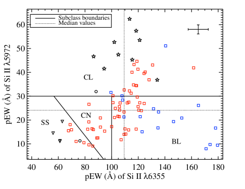
Figure 10: The pEW of Si ii $\lambda$5972 versus the pEW of Si ii $\lambda$6355 of 89 SNe. Colours and shapes of data points are the same as in Figure 4. The solid lines are the boundaries between the four classes from Branch et al. (2009): CN = core normal, BL = broad line, CL = cool, SS = shallow silicon. The dotted lines are the median values of the two features’ pEWs. The median uncertainty in both directions is shown in the upper-right corner.

A slightly larger range of spectral ages than what was used by Branch et al. (2009) is adopted here in order to increase the number of objects studied. The classifications and general trends seen when using only spectra within 3 d of maximum brightness are preserved when spectra within 5 d of maximum are used. Conversely, if a larger range of ages is used, the pEWs of the Si ii $\lambda$5972 and Si ii $\lambda$5972 features begin to evolve noticeably. The trends seen in Figure 10 are also visible at similar levels when plotting $\Delta$pEW values (instead of pEW values), but by definition $\Delta$pEW relies on a fit to the measurements as opposed to the measurements themselves. Finally, when the BSNIP dataset contains multiple spectra of a given object within 5 d of maximum, only the spectrum nearest maximum brightness is used. This also has little to no effect on the classification of any SNe, nor on the trends seen in Figure 10.

One distinction between the two studies is that the BSNIP sample is lacking some of the most extreme members of the SS subclass. Most of these objects are the extremely peculiar SN 2000cx and SN 2002cx-like objects which are ignored in this study a priori. Other SNe in the bottom-left corner of Figure 2 of Branch et al. (2009) are Ia-91T, and even though there are a handful of Ia-91T SNe in the dataset presented here, the BSNIP sample does not contain spectra of any of these objects within 4 d of maximum. It does, however, include four Ia-99aa objects plotted in Figure 10 (SNe 1998es, 1999aa, 1999dq, 2001eh) which are thought to be intermediate objects between Ia-91T and Ia-norm (e.g., Garavini et al., 2004). They are much less clustered than they are in Branch et al. (2009), even though SN 1998es and SN 2001eh lie nearly on top of each other in Figure 10. The other major difference between this sample and that of Branch et al. (2009) is the relative number of objects in each class. Even though the total number of SNe is comparable in the two datasets, the BSNIP sample has significantly more CL and BL objects, mostly at the expense of CN objects (if one accounts for the fact that we are biased against some of the extreme SS SNe as mentioned above).

One of the most striking trends seen in Figure 10 is that all of the data seem to form a nearly continuous, fairly well-correlated distribution with the most spectroscopically peculiar objects lying at the extreme edges of the distribution. We have no Ia-91T objects in the figure, but they would fall in the bottom-left corner. From there, as the pEW of Si ii $\lambda$6355 increases at approximately constant Si ii $\lambda$5972 pEW, we find the Ia-99aa, then Ia-norm, and finally HV SNe. Similarly, if we start at the median pEW values for the two features (where the dotted lines cross in Figure 10), and increase Si ii $\lambda$5972 pEW at constant Si ii $\lambda$6355, we first find (mostly) Ia-norm and then the Ia-91bg objects. This amount of separation between SN Ia subclasses is not seen when comparing the pEWs of any other pair of features measured here. However, a somewhat weaker version of this separation is seen when comparing the pEW of Si ii $\lambda$6355 to the pEW of both Ca ii H&K and the S ii “W.” In addition, Ia-91bg objects are found to distinguish themselves from the other subclasses mentioned here when comparing pEW values from a few pairs of spectral features.

The subtypes used here (excluding HV) come from SNID, which cross-correlates the entire input spectrum with a library of SN spectra of various subtypes. However, it appears that we can classify the vast majority of SNe Ia using only the pEWs of these two Si ii features, as opposed to a spectrum covering a much wider wavelength range. The fact that there seems to be a continuous distribution in these pEW values with the most spectroscopically peculiar objects on the edges of the distribution indicates that the often-used spectral classification scheme based on Ia-91bg, Ia-norm, and Ia-91T objects may only accurately represent the most extreme objects. In other words, an object spectrally classified as Ia-norm might in reality have some observables in common with Ia-norm and some in common with one of the peculiar subtypes. This classification scheme, while being somewhat qualitative in nature, is still useful, however, since any object spectroscopically classified as peculiar will be an outlier in the population of all SNe Ia, and it is often by studying the most extreme cases that one learns the most. A deeper, quantitative investigation into the photometric and host-galaxy properties of these spectroscopically determined subclasses will be undertaken in BSNIP III and other papers in this series.

5.6 The Si II Ratio

The so-called “Si ii ratio,” $\Re$(Si ii), was defined by Nugent et al. (1995) as the ratio of the depth of the Si ii $\lambda$5972 feature to the depth of the Si ii $\lambda$6355 feature. In our notation this is $a$(Si ii $\lambda$5972) / $a$(Si ii $\lambda$6355). They present a spectroscopic and photometric sequence of SNe Ia based on temperature differences which they attribute to differences in the total amount of ⁵⁶Ni produced in the explosion. The Si ii ratio has been previously found to correlate with absolute $B$-band magnitude (Nugent et al., 1995), $\Delta m_{15}$ (Benetti et al., 2005; Hachinger et al., 2006), $\left(B-V\right)_{0}$ (Altavilla et al., 2009), and colour-corrected Hubble residual (Blondin et al., 2011). We will explore some of these relationships in BSNIP III.

While Nugent et al. (1995) originally defined the Si ii ratio using the depths of spectral features, Hachinger et al. (2006) define the Si ii ratio using the pEWs of the Si ii $\lambda$5972 and Si ii $\lambda$6355 lines. With their redefined Si ii ratio, Hachinger et al. (2006) observe a similar trend to what was found by Nugent et al. (1995): brighter SNe Ia with broader light curves have smaller Si ii ratios. In Figure 11 we investigate how consistent the Si ii ratio is when defined using spectral feature depths (ordinate) versus pEWs (abscissa). The linear least-squares fit to all 162 points is shown as a solid line while the RMSE of the fit is shown as the dashed lines.

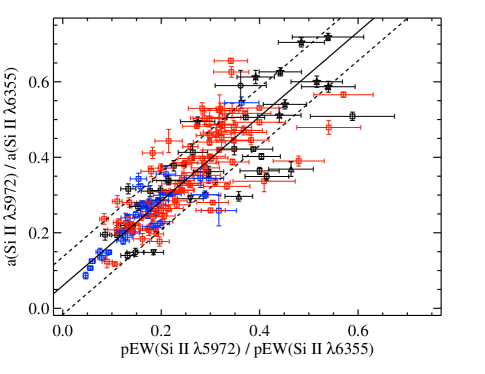
Figure 11: The Si ii ratio defined using spectral feature depth versus the Si ii ratio defined using pEWs for 162 SNe. Colours and shapes of data points are the same as in Figure 4. The solid line is the linear least-squares fit and the dashed lines are the RMSE of the fit. The Spearman rank coefficient is $\sim\!\!$ 0.86.

The two different ways to define the Si ii ratio appear to be well correlated; the Spearman rank coefficient is $\sim\!\!$ 0.86. According to the fit, the zero-point offset between the two is $\sim\!\!$ 0.06, though this should formally be zero since if the pEW is zero then the feature’s depth is also zero. To measure the spectral feature depth one must determine the minimum of the spectral feature (either by smoothing the data or fitting a function to the flux, in order to avoid local, unphysical minima due to noise) and then define the feature’s endpoints and a pseudo-continuum to compare to the flux at the minimum. However, to measure a pEW, one only needs to define the endpoints and a pseudo-continuum. Therefore, the pEW is a more robust and easier to measure parameter than the spectral feature depth, and since they are well correlated we will follow Hachinger et al. (2006) and define the Si ii ratio as

$$\Re\left(\textrm{\text{Si\,{ii}}}\right)\equiv\frac{\textrm{pEW}\left(\textrm{\text{Si\,{ii}} $\lambda$5972}\right)}{\textrm{pEW}\left(\textrm{\text{Si\,{ii}} $\lambda$6355}\right)}.$$ (3)

The temporal evolution of the Si ii ratio is shown in Figure 12, where we have once again colour-coded the data based on their HV or normal-velocity classification and shape-coded the data based on their SNID classification. There is a significant amount of scatter in $\Re$(Si ii) and thus it is difficult to discern whether there is much temporal evolution for any of the subclasses of SNe Ia. The one point that can be fairly robustly made from inspecting Figure 12 is that Ia-91bg objects consistently have the largest Si ii ratios. This partially matches what has been previously seen in that fainter SNe Ia with narrow light curves (oftentimes spectroscopically resembling SN 1991bg) tend to have large $\Re$(Si ii) values (e.g., Nugent et al., 1995; Benetti et al., 2005; Hachinger et al., 2006). However, these previous results also show that more luminous objects with broader light curves have the smallest Si ii ratios, which is not readily apparent in the current study. There are only a few Ia-91T/99aa SNe plotted in Figure 12, but they all have average values of $\Re$(Si ii).

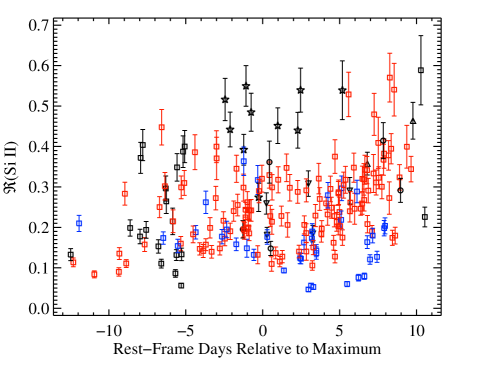
Figure 12: The Si ii ratio versus rest-frame age relative to maximum brightness of 200 spectra of 154 SNe Ia. Colours and shapes of data points are the same as in Figure 4.

Figure 12 also suggests that HV objects may have, on average, lower Si ii ratios than SNe with normal velocities, although the large scatter renders this conclusion tentative at best. When colour-coding the data by “Benetti type,” as expected the FAINT objects have the highest values of $\Re$(Si ii) (since they are defined as SNe having the narrowest light curves). Somewhat different than previous studies is that LVG and HVG objects all have approximately the same values of the Si ii ratio. Furthermore, while we only have a handful of objects with a measured $\Re$(Si ii) at $t<-5$ d, a few are LVG and a few are HVG, and they all have approximately average values of the Si ii ratio. This is markedly different than reported by Benetti et al. (2005), whose data show that HVG objects have larger than average $\Re$(Si ii) values at these earliest epochs (though they do decrease to more typical values at later times).

The pEW of the Si ii $\lambda$5972 feature and the Si ii ratio have both been found to correlate well with $\Delta m_{15}$ (e.g., Nugent et al., 1995; Hachinger et al., 2006). Hachinger et al. (2006) point out (from their Fig. 10) that each of these correlations implies the other’s existence based on the relationship between the near-maximum values of pEW of Si ii $\lambda$5972 and $\Re$(Si ii). In Figure 13 the pEW of the Si ii $\lambda$5972 feature versus the Si ii ratio is plotted for objects within 5 d of maximum, confirming this correlation. The plot contains 89 SNe Ia. If the current dataset had multiple spectra of a given object for which $\Re$(Si ii) and the pEW of the Si ii $\lambda$5972 feature was calculated, the observation closest to maximum brightness was used. Thus, in Figure 13, there is one data point per object. This practice of using only the spectrum nearest to maximum brightness when multiple spectra of a given object are analysed is followed in the rest of this work unless otherwise noted.

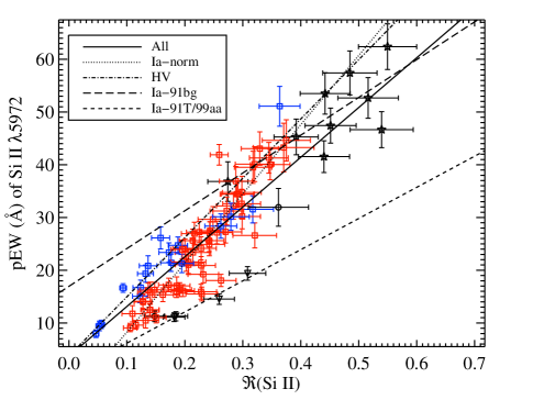
Figure 13: The pEW of the Si ii $\lambda$5972 feature versus the Si ii ratio for 89 SNe Ia. Colours and shapes of data points are the same as in Figure 4. The various lines are fits to all of the data (solid), only Ia-norm objects (dotted), only HV objects (dot-dashed), only Ia-91bg objects (long-dashed), and only Ia-91T/99aa objects (short-dashed). All of the fits have Spearman rank coefficients of $>0.89$ except the Ia-91bg objects (which have a coefficient of $\sim\!\!$ 0.79).

In Figure 13 the current study’s definition of $\Re$(Si ii) is used (i.e., the ratio of pEWs) as opposed to the original definition (i.e., the ratio of depths; Nugent et al., 1995). Figure 10 of Hachinger et al. (2006) uses the original definition on the abscissa. When the original definition is used with the BSNIP data, results qualitatively similar to those of Figure 13 are seen. Hachinger et al. (2006) interpolate/extrapolate their pEW measurements to $t=0$ d, while spectra within 5 d of maximum brightness (as in Section 5.5) are used in Figure 13 since the pEWs of the Si ii $\lambda$5972 and Si ii $\lambda$5972 features do not change much during these epochs. If the few objects with spectra earlier than 5 d before maximum are included, they fall along the linear correlation. However, if objects with spectra later than 5 d after maximum are added, they mainly fall below the linear correlation. This is due to the fact that the Si ii $\lambda$5972 pEW values remain relatively constant for $t\la 5$ d but begin to increase at later times, as seen in Figure 7 (bottom left).

As mentioned above, Ia-91bg objects have large Si ii ratios and large Si ii $\lambda$5972 pEWs, and are thus found in the upper right of the linear correlation in Figure 13. Conversely, it was shown that Ia-91T/99aa SNe have low values of Si ii $\lambda$6355 pEW and low-to-average values of Si ii $\lambda$5972 pEW, so one may expect them to lie at the bottom left of the correlation, and in fact it appears that these objects lie somewhat below the main correlation. The HV SNe perhaps make up the upper part of the main correlation, with the normal-velocity objects making up the lower part, though these two groups are fairly well mixed. Similarly, if we code the points in Figure 13 by velocity gradient, we see that the HVG objects usually lie slightly above the LVG objects (as seen in Hachinger et al., 2006), but with a significant amount of overlap. The FAINT objects in the BSNIP sample are found at the upper right of the correlation, as seen previously (Hachinger et al., 2006), and reinforce the connection between Ia-91bg SNe and FAINT SNe.

To investigate whether the various subclasses have distinct correlations, linear functions were fit to all of the data in Figure 13 as well as each individual subclass. All of the fits have Spearman rank coefficients of $>0.89$ except the Ia-91bg objects (which have a coefficient of $\sim\!\!$ 0.79), implying that each subclass, and the data as a whole, are well fit by a linear function (though Ia-91bg SNe have a fair amount of scatter). The linear fit to all of the data and the linear fits to the Ia-norm, HV, and Ia-91bg objects are all consistent with each other at the 2$\sigma$ level. As mentioned above, the Ia-91T/99aa SNe fall below the main correlation and appear to lie on their own relationship. However, since there are only four points in the fit, it is difficult to say if this difference is statistically significant. Previous work has indicated that both the pEW of the Si ii $\lambda$5972 feature and the Si ii ratio are luminosity indicators (e.g., Hachinger et al., 2006). The scatter in the relationship between these two parameters may be related to differences in luminosity or light-curve shape (i.e., Ia-norm versus Ia-91bg versus Ia-91T) or differences in velocity (i.e., HV versus normal velocity), which might also be related to differences in colour (Foley & Kasen, 2011). Adding photometric observables such as these into this analysis will be done in BSNIP III.

The pEW of the Si ii $\lambda$4000 feature has also been used as a luminosity indicator (Arsenijevic et al., 2008; Walker et al., 2011; Blondin et al., 2011; Chotard et al., 2011). Therefore, one might expect it to also correlate well with the Si ii ratio. Figure 14 shows the pEW of the Si ii $\lambda$4000 feature versus $\Re$(Si ii) for objects within 5 d of maximum brightness. The plot contains 66 SNe Ia.

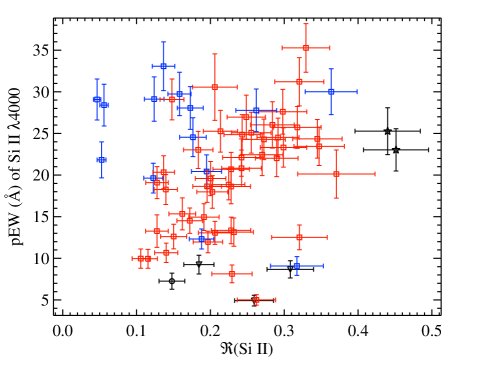
Figure 14: The pEW of the Si ii $\lambda$4000 feature versus the Si ii ratio for 66 SNe Ia. Colours and shapes of data points are the same as in Figure 4.

Figure 14 shows no obvious correlation between pEWs of the Si ii $\lambda$4000 feature and $\Re$(Si ii). As in Figure 13, Ia-91bg are found to have the highest Si ii ratio and are thus toward the right of the figure, while the Ia-91T/99aa SNe have small pEWs in general and are thus found toward the bottom of the plot. The HV objects have higher-than-average Si ii $\lambda$4000 pEW values with relatively low Si ii ratios, but they overlap quite a bit with the normal-velocity objects. The Ia-norm SNe show the most consistent relationship between these two parameters, although they have a large scatter and a Spearman rank coefficient of only $\sim\!\!$ 0.51. The fact that these two spectroscopic observables are both used as luminosity indicators (e.g., Blondin et al., 2011) and yet they are seemingly uncorrelated is curious. Further investigation into this discrepancy (with the addition of luminosity information for some of the SNe presented here) will take place in BSNIP III.

5.7 Other pEW and Flux Ratios

5.7.1 The Ca ii Ratio

Similar to the Si ii ratio, Nugent et al. (1995) defined the Ca ii ratio as the ratio of the flux at the red edge of the Ca ii H&K feature to the flux at the blue edge of that feature. In our notation this is defined as

$$\Re\left(\textrm{\text{Ca\,{ii}}}\right)\equiv\frac{F_{r}\left(\textrm{\text{Ca\,{ii}}~{}H\&K}\right)}{F_{b}\left(\textrm{\text{Ca\,{ii}}~{}H\&K}\right)}.$$ (4)

They found that this parameter scaled with absolute $B$-band magnitude in the same way as $\Re$(Si ii). The Ca ii ratio has been investigated further in more recent studies, and while there is not much temporal evolution of the parameter within 5 d of maximum brightness (Bongard et al., 2006), it is unclear whether this spectral parameter is reasonably well correlated with luminosity (Blondin et al., 2011).

Since the Si ii ratio and the Ca ii ratio have both been shown to correlate with absolute $B$-band magnitude (Nugent et al., 1995; Bongard et al., 2006), one might expect the two ratios to correlate with each other. However, we find no significant correlation.

5.7.2 The “SiS” Ratio

Somewhat analogous to the Ca ii ratio, Bongard et al. (2006) defined the “SiS ratio” as the ratio of the flux at the red edge of the S ii “W” feature to the flux at the red edge of the Si ii $\lambda$6355 feature. This is defined using our notation as

$$\Re\left(\textrm{SiS}\right)\equiv\frac{F_{r}\left(\textrm{\text{S\,{ii}} ``W''}\right)}{F_{r}\left(\textrm{\text{Si\,{ii}} $\lambda$6355}\right)}.$$ (5)

This parameter was shown to scale with absolute $B$-band magnitude in the same way as $\Re$(Ca ii). Even though Bongard et al. (2006) make a time-dependent correction to yield this correlation, they state that the existence of a universal time correction for this ratio is doubtful. In fact, very little temporal evolution of $\Re$(SiS) near maximum brightness is seen in the BSNIP data. The SiS ratio has been measured for more objects in recent work, but it does not appear to correlate as well with luminosity as initially claimed (Blondin et al., 2011).

Since the SiS ratio and the Si ii ratio have both been shown to correlate with absolute $B$-band magnitude (Bongard et al., 2006), one might expect the two ratios to correlate with each other. Effectively no evidence for such a correlation is found in the current dataset.

One may expect the SiS ratio to be related to the pEW of the S ii “W” feature or the Si ii $\lambda$6355 feature (or perhaps the ratio of the two). We find no evidence for such a correlation with the pEW of the S ii “W” alone, but a possible relationship exists between $\Re$(SiS) and the pEW of the Si ii $\lambda$6355 feature, as well as the ratio of the pEW of the S ii “W” to that of Si ii $\lambda$6355. Figure 15 presents 110 SNe within 5 d of maximum brightness for which we measure $\Re$(SiS). Increasing or decreasing the age range investigated does not change the basic trends seen in Figure 15.

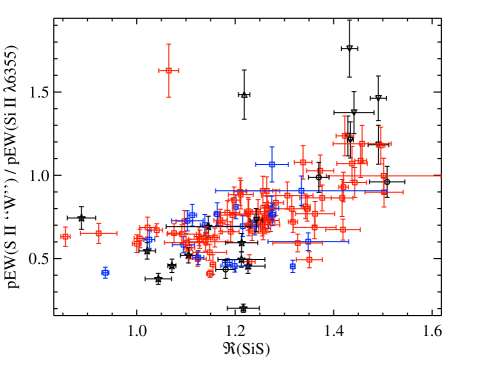
Figure 15: The ratio of the pEW of S ii “W” to that of Si ii $\lambda$6355 versus SiS ratio for 110 SNe Ia. Colours and shapes of data points are the same as in Figure 4.

It is possible that the SiS ratio is linearly (or quadratically) related to the ratio of pEWs, but there is a significant amount of scatter in Figure 15. Interestingly, Ia-91bg and Ia-99aa objects once again tend to lie on the outskirts of the distribution, but there is much overlap with the HV and Ia-norm objects (which are nearly indistinguishable in this parameter space). There are also a few extreme outliers in Figure 15, including the lone Ia-91T object plotted. When comparing $\Re$(SiS) to the pEW of Si ii $\lambda$6355 alone, the same separations (or lack thereof) between the different subclasses once again appear, as do the same outliers. The only difference is that the two values are (possibly) linearly anticorrelated.

5.7.3 The “SSi” Ratio

Another parameter that has been proposed as a spectroscopic luminosity indicator is the ratio of the pEW of the S ii “W” to that of the Si ii $\lambda$5972 feature (Hachinger et al., 2006). They found that this ratio, dubbed $\Re$(S,Si), is linearly anticorrelated with $\Delta m_{15}$ (which is opposite the relationship between $\Re$(Si ii) and $\Delta m_{15}$). Following Hachinger et al. (2006), we define the “SSi ratio” as

$$\Re\left(\textrm{S,Si}\right)\equiv\frac{\textrm{pEW}\left(\textrm{\text{S\,{ii}} ``W''}\right)}{\textrm{pEW}\left(\textrm{\text{Si\,{ii}} $\lambda$5972}\right)}.$$ (6)

There is strong evidence for an anticorrelation between the Si ii ratio and the SSi ratio in Figure 16, which presents the 85 SNe (within 5 d of maximum) for which both $\Re$(S,Si) and $\Re$(Si ii) are measured.

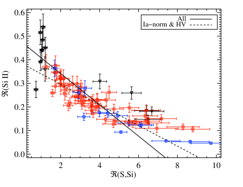
Figure 16: The Si ii ratio versus the SSi ratio for 85 SNe Ia. Colours and shapes of data points are the same as in Figure 4. The solid line is a linear fit to all of the data and the dashed line is a linear fit to only the Ia-norm and HV objects. The Spearman rank coefficient for both the entire dataset as well as only the Ia-norm and HV objects is approximately $-0.89$.

Interestingly, the overall correlation (and differences between different subclasses) is unchanged when we include data from all epochs studied in this work. It is also unchanged when a narrower age range is used. The overall anticorrelation seen in Figure 16 suggests that $\Re$(S,Si) may indeed be as good a luminosity indicator as $\Re$(Si ii), though recent work suggests otherwise (Blondin et al., 2011). While the trend for all objects shown in Figure 16 may not be linear, they do appear well correlated, with a Spearman rank coefficient of about $-0.89$. A linear fit to all 85 SNe in Figure 16 is shown by the solid line. A linear fit to only the Ia-norm and HV objects is shown by the dashed line in Figure 16; this subset has a nearly identical Spearman rank coefficient to that of the entire sample. The tantalising possibility that $\Re$(S,Si) is yet another spectral luminosity indicator will be explored further in BSNIP III.

5.7.4 The “SiFe” Ratio

Similar to the SSi ratio, Hachinger et al. (2006) also found that the ratio of the pEW of the Si ii $\lambda$5972 feature to that of the Fe ii complex can be used as a spectroscopic luminosity indicator since it scaled linearly with $\Delta m_{15}$. They referred to this as the “SiFe ratio,” defined as

$$\Re\left(\textrm{Si,Fe}\right)\equiv\frac{\textrm{pEW}\left(\textrm{\text{Si\,{ii}} $\lambda$5972}\right)}{\textrm{pEW}\left(\textrm{\text{Fe\,{ii}}}\right)}.$$ (7)

There is also strong evidence for a correlation between the Si ii ratio and the SiFe ratio in Figure 17, where the 72 SNe (within 5 d of maximum) are shown for which both $\Re$(Si,Fe) and $\Re$(Si ii) are measured.

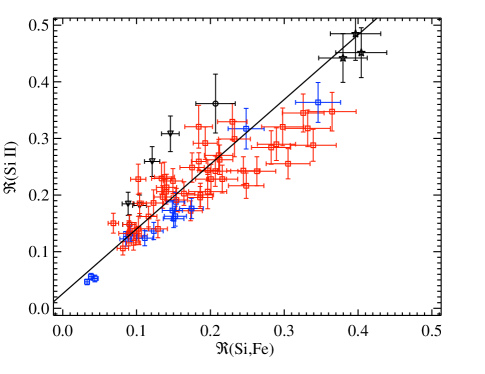
Figure 17: The Si ii ratio versus the SiFe ratio for 72 SNe Ia. Colours and shapes of data points are the same as in Figure 4. The solid line is a linear fit to all of the data and the Spearman rank coefficient is $\sim\!\!$ 0.86.

The scatter in the relationship between the Si ii ratio and the SiFe ratio increases when including data from all epochs studied here. The overall correlation seen in Figure 17 suggests that $\Re$(Si,Fe) may also be an accurate luminosity indicator, though Blondin et al. (2011) report that it does not significantly improve the accuracy of their luminosity determinations. The data are well fit by a linear function and are highly correlated (Spearman rank coefficient of $\sim\!\!$ 0.86); a linear fit to all 72 SNe in Figure 16 is shown by the solid line. The Ia-91bg objects distinguish themselves quite prominently except the lone point that appears to be closer to the Ia-99aa objects, which are also found at an outer edge of the main relationship. The HV SNe tend to be at the bottom of the relationship, with a handful of significant outliers. The use of $\Re$(Si,Fe) as a luminosity indicator will be investigated further in BSNIP III.

5.8 Comparing Expansion Velocities to Pseudo-Equivalent Widths

In Section 5.4.7 the possibility of a correlation between expansion velocity and pEW was mentioned, at least for the Ca ii H&K, Mg ii, Fe ii, and Si ii $\lambda$6355 features. The pEW for these four features is plotted versus the expansion velocity of Si ii $\lambda$6355 in Figure 18. They contain all objects with spectra obtained within 5 d of maximum brightness. In all cases, decreasing the age range investigated does not change the basic trends seen in the figure, though increasing the age range increases the overlap among the various subclasses. Again, we plot values only from the spectrum closest to maximum brightness for each SN Ia and thus there is one data point per object.

$\begin{array}[]{cc}\includegraphics[width=252.94499pt]{ew_vsi6355_cahk}&\includegraphics[width=252.94499pt]{ew_vsi6355_mg}\\ \includegraphics[width=252.94499pt]{ew_vsi6355_fe}&\includegraphics[width=252.94499pt]{ew_vsi6355_si6355}\\ \end{array}$

Figure 18: The pEW of various spectral features versus the velocity of Si ii $\lambda$6355. (top left) 92 SNe Ia for Ca ii H&K, (top right) 99 SNe Ia for the Mg ii complex, (bottom left) 99 SNe for the Fe ii complex, and (bottom right) 120 SNe for Si ii $\lambda$6355. Colours and shapes of data points are the same as in Figure 4. The median uncertainty in both directions is shown in the lower-right corner of each panel. In the bottom-right panel the filled blue square is the HV object SN 2006X which shows evidence for interaction with circumstellar material (Patat et al., 2007) and an aspherical explosion (Patat et al., 2009), and the filled black squares are the HV objects SNe 2002bf, 2002bo, and 2004dt, all of which show evidence for an aspherical explosion via large Si ii polarizations (Wang et al., 2006).

By construction, HV objects are always found toward the right-hand side of plots of pEW versus Si ii $\lambda$6355 velocity. But, as hinted in Section 5.4.7, they also have higher-than-average pEW values for most of the spectral features investigated. The features showing the greatest differentiation between Ia-norm and HV objects in this parameter space are the four mentioned above and plotted in Figure 18.

In each of these four Figures there is significant overlap among spectroscopically peculiar objects and Ia-norm, while the HV SNe tend to be fairly well separated. However, there is a large scatter, and thus it is difficult to say whether there is any real correlation between pEW and Si ii $\lambda$6355 velocity for the Ia-norm and the HV objects. The Spearman rank coefficients for the panels in Figure 18 are all about 0.21–0.35. Using only the Ia-norm and HV objects, the Spearman rank coefficients improve only moderately for these spectral features (0.28–0.33).

The bottom-right panel of Figure 18 shows the largest difference between the various subclasses of SNe Ia, although there is still much overlap (mostly between Ia-norm and Ia-91bg objects). There is a more significant correlation between the pEW of Si ii $\lambda$6355 and the expansion velocity derived from that same feature (Spearman rank coefficient of 0.43 for all objects in the bottom-right panel of Figure 18 and 0.51 for Ia-norm and HV SNe only). The basic trend seen in this figure has also been noted previously by Wang et al. (2009) with some of the same spectra used in this study. Their plot shows only SNe Ia within 3 d of maximum while Figure 18 presents objects within 5 d of maximum. Wang et al. (2009) point out that HV objects typically have pEW values greater than $\sim\!\!$ 100 Å, which is also observed here.

The observation of a strong Si ii $\lambda$6355 feature at high velocities may indicate an enhancement in the abundance or density in the outermost layers of HV objects. This could be caused by an extended burning front, different degrees of mixing in the ejecta, or interaction with circumstellar material (CSM; Benetti et al., 2004; Wang et al., 2009). In fact, two SNe Ia with some of the best direct observational evidence for CSM interaction, SN 2006X (Patat et al., 2007, the filled blue square in the bottom-right panel of Figure 18) and SN 2007le (Simon et al., 2009), are both in the current sample and are found to be HV objects.

Wang et al. (2009) also point out that the distribution of pEWs and velocities between Ia-norm and HV objects is continuous, and therefore it is likely that the proposed enhancement occurs at a wide range of values (with the majority of SNe Ia showing relatively low levels of this enhancement). They suggest that this could be a result of viewing angle effects if HV objects are associated with asymmetric structures. There is both observational (Leonard et al., 2005; Wang et al., 2006) and theoretical (Maeda et al., 2010) evidence that HV SNe may be associated with certain viewing angles of aspherical explosions.

Leonard et al. (2005), Wang et al. (2007), and Patat et al. (2009) discuss spectropolarimetric data on SNe 1997bp, 2002bf, 2002bo, 2004dt, 2004ef, and 2006X, all of which show large Si ii polarizations, implying an asymmetric explosion. These objects are found to be HV SNe in the BSNIP data; SNe 2002bf, 2002bo, and 2004dt are plotted as filled black squares in the bottom-right panel of Figure 18 and SN 2006X is plotted as a filled blue square. Building on the work of Leonard et al. (2005), Maund et al. (2010) found a correlation between the level of Si ii polarization and $\dot{v}$. Of the six aforementioned HV SNe with large polarizations, the two for which we measure a velocity gradient are both HVG objects. Si ii $\lambda$6355 velocity, $\dot{v}$, and level of polarization may all also be correlated with velocity offsets of nebular lines in late-time spectra (Maeda et al., 2010). Comparisons of spectra at later epochs to models such as those presented by Maeda et al. (2010) will be made in future BSNIP studies.

6 Conclusions

This is the second paper in the BSNIP series, and it presents spectral feature measurements of 432 low-redshift ($z<0.1$) optical spectra within 20 d of maximum brightness of 261 SNe Ia. These data all come from BSNIP I (Silverman et al., 2012) and were obtained from 1989 through the end of 2008. We have outlined in detail our automated and robust procedure for spectral feature definition and measurement which has expanded upon the work of previous studies. Using this algorithm we attempted to measure expansion velocities, pEWs, spectral feature depths, and fluxes at the centre and endpoints of each of nine major spectral feature complexes. The raw numbers measured from the data are also presented. A sanity check of the consistency of our measurements was performed using the BSNIP data in addition to the spectra presented by Matheson et al. (2008). Even though the current study utilises spectral data almost exclusively, future BSNIP papers will incorporate photometric data and host-galaxy properties into the measurements discussed in this work.

6.1 Summary of Spectral Feature Measurements

The temporal evolution of the expansion velocity of each of the spectral features (except for the Mg ii and Fe ii complexes) was explored. The observed differences in velocities support the layered structure of SN Ia ejecta, with Ca ii found in the outermost (i.e., fastest expanding) layers and O i, Si ii, and S ii found in the inner (i.e., slower expanding) layers. Many of the basic trends seen previously are confirmed by the current analysis, including evidence of a HV population of spectroscopically normal SNe (Wang et al., 2009). A sharp cutoff between normal-velocity and HV objects is not well motivated by the data analysed here, though there are some differences between spectroscopically normal SNe Ia with the lowest and highest velocities near maximum brightness (which is discussed in more detail below).

Following Benetti et al. (2005), velocity gradients are calculated and then used (along with light-curve shape, for those that have that information) in order to classify the SNe. The BSNIP dataset is not the best suited for this kind of study due to the relatively low number of spectra per object. However, $\dot{v}$ is still measured for 61 objects.

The interpolated/extrapolated velocity at maximum brightness ($v_{0}$) and at 10 d past maximum ($v_{10}$) was calculated for each SN with a measured $\dot{v}$. Effectively no correlation is found between $v_{10}$ and velocity-gradient classification, and only a weak correlation is seen between $v_{0}$ and velocity gradient. In previous work HV and HVG objects have been used almost interchangeably, as have normal-velocity and LVG objects (e.g., Hachinger et al., 2006; Pignata et al., 2008; Wang et al., 2009). However, the data presented here cast serious doubt on these associations.

The temporal evolution of the pEW of each spectral feature was also examined. As in Nordin et al. (2011b), $\Delta$pEW was calculated by subtracting a fit to the data from the measurements themselves. Unlike previous work, only linear and quadratic functions were used to fit the temporal evolution. However, the $\Delta$pEW values rely on defining a fit (either linear or quadratic) to the measurements, adding another assumption to the analysis. No correlation between velocity gradient and pEW or $\Delta$pEW is seen in the data presented here, even though there has been evidence presented previously for a relationship between $\Delta$pEW of the Si ii $\lambda$4000 feature and $\dot{v}$ (Nordin et al., 2011a).

We use pEW values of Si ii $\lambda$6355 and Si ii $\lambda$5972 to classify the BSNIP data according to the four groups defined by Branch et al. (2006). The boundaries between these groups appear to be arbitrary in the context of the spectral measurements presented here. That being said, spectroscopically peculiar SNe Ia and HV objects occupy the outermost edges of the nearly continuous parameter space filled in by the Ia-norm objects. Thus, the “SNID types” seem to be the most extreme versions of the three non-CN “Branch types.” Furthermore, both of these classification schemes are quasi-arbitrary cuts in what appears to be a continuous distribution of pEW values.

It was shown that the Si ii ratio can be equivalently defined as a ratio of spectral feature depths or pEW values and the latter is used as the definition for the present study. This quantity has been shown to correlate with a variety of photometric observables (e.g., Nugent et al., 1995; Hachinger et al., 2006; Altavilla et al., 2009; Blondin et al., 2011) and these proposed relationships will be investigated further in BSNIP III. We do confirm the observation that Ia-91bg objects (often underluminous) have the largest $\Re$(Si ii) values. On the other hand, the Ia-91T/99aa objects (often overluminous) seem to have average $\Re$(Si ii) values, which differs from what has been previously seen (e.g., Hachinger et al., 2006).

Benetti et al. (2005) presented evidence of HVG objects having the largest measured Si ii ratios at $t<-5$ d, though the few objects for which we measure $\Re$(Si ii) at these early epochs all have quite typical Si ii ratios and represent the LVG and HVG classes. The pEW of the Si ii $\lambda$5972 feature and $\Re$(Si ii) have both been found to correlate well with $\Delta m_{15}$ (e.g., Nugent et al., 1995; Hachinger et al., 2006), and the BSNIP data show strong evidence of a linear correlation between these spectral parameters. While the HV and Ia-norm objects show quite a bit of overlap in this parameter space, the Ia-91bg objects lie at the uppermost end of the correlation and the Ia-91T/99aa objects are well below the main trend (and perhaps form there own, distinct relationship).

Four other pEW and flux ratios were also calculated and discussed. Two of these, the Ca ii ratio and SiS ratio, have been previously seen to be correlated with $B$-band magnitude in the same way as the Si ii ratio (Nugent et al., 1995; Bongard et al., 2006, respectively). However, no relationship between $\Re$(Si ii) and $\Re$(Ca ii) is seen here, and only a weak relationship is observed between $\Re$(Si ii) and $\Re$(SiS). The various “SNID types” and “Wang types” all have similar ranges of Ca ii and SiS ratios. The other two ratios investigated, the SSi ratio and the SiFe ratio, were shown by Hachinger et al. (2006) to be anticorrelated and correlated with $\Delta m_{15}$, respectively. There is strong evidence that both of these ratios are correlated with $\Re$(Si ii) in the BSNIP data. Most of the “SNID types” and “Wang types” have a high degree of overlap in the plots of Si ii ratio versus SSi ratio and SiFe ratio, and the Ia-91bg objects occupy the extreme upper end of both of these correlations.

Finally, possible correlations between the expansion velocity of Si ii $\lambda$6355 and pEWs of Ca ii H&K, Mg ii, Fe ii, and Si ii $\lambda$6355 were explored. Spectroscopically peculiar objects mostly overlap with Ia-norm objects in these plots, while the HV SNe show both higher expansion velocities and pEW values. CSM interaction and asymmetric explosions have been proposed to explain the existence of SNe Ia with high velocities and large pEWs (Benetti et al., 2005; Wang et al., 2006, respectively). Interestingly, four of the points at the uppermost end of the Si ii $\lambda$6355 velocity-pEW relationship show evidence for CSM interaction (SN 2006X) or an aspherical explosion (SNe 2002bf, 2002bo, and 2004dt).

6.2 Can a Theoretical Model of SNe Ia Explain Their Spectra?

Many of the spectral measurements investigated in this study show a continuous (or nearly so) range of values. This is perhaps evidence that all of the SN Ia subclasses considered here can be described by one, self-consistent physical model that only varies in one or two intrinsic parameters. It was suggested well over a decade ago that the Ia-91bg, Ia-norm, and Ia-91T/99aa objects can be naturally linked through a continuous increase in temperature, presumably by a smoothly increasing amount of ⁵⁶Ni produced in the explosion (e.g., Nugent et al., 1995). More recently, it has been suggested that continuous variations in viewing angle can give rise to HV and normal-velocity objects (Kasen & Plewa, 2007; Kasen et al., 2009; Maeda et al., 2010). Any model that hopes to reflect reality must match the observed spectral properties near maximum brightness (as presented here), as well as the photometric observations of SNe Ia (as shown by Ganeshalingam et al., 2010, and discussed further in BSNIP III).

Perhaps by varying both the amount of ⁵⁶Ni produced and the viewing angle, one can self-consistently explain all of the subclasses of SNe Ia (and their measured spectral parameters). Though tantalizing, a deeper investigation of this possibility is beyond the scope of this paper. Furthermore, if one (or more) of the subclasses of SNe Ia are in reality fundamentally different, then discussing only a single theoretical model does not make sense. At least two distinct progenitor channels (possibly resulting in different observed spectra) have been suggested for SNe Ia: the single degenerate (e.g., Whelan & Iben, 1973) and the double degenerate (e.g., Iben & Tutukov, 1984; Webbink, 1984). Similarly, different types of SNe Ia may be found in different host galaxies (perhaps related to host-galaxy type, mass, metallicity, or stellar age; e.g., Gallagher et al., 2008; Hicken et al., 2009; Howell et al., 2009), which may also point to multiple models being required to explain all of the observed spectra.

6.3 What About Future SN Surveys?

Surveys which are much larger than BSNIP and tuned to discovering the bulk of their SNe Ia at higher redshifts than BSNIP are already underway (e.g., Rau et al., 2009; Law et al., 2009; Kaiser et al., 2002), with many more planned for the future (e.g., LSST, WFIRST, Euclid). With such large numbers of objects being discovered, it will be extremely difficult to obtain high-quality light curves and/or multiple spectra of most SNe. Instead, one will need to rely on only a handful of photometric points and perhaps one, often relatively low S/N, spectrum. Thus, photometric luminosity indicators in combination with spectral indicators that can be measured in one low-quality spectrum will be important.

For higher-$z$ surveys in particular, useful spectral features that are found toward the blue end of the optical range will be even more critical. For $z\ga 0.6$, the red wing of the typical, near-maximum Si ii $\lambda$6355 feature becomes redshifted beyond $\sim\!\!$ 1 $\mu$m. The Ca ii ratio and the pEW of the Si ii $\lambda$4000 feature are promising in this regard and both have been found to correlate with light-curve width (e.g., Nugent et al., 1995; Bongard et al., 2006; Arsenijevic et al., 2008; Walker et al., 2011; Blondin et al., 2011; Nordin et al., 2011b; Chotard et al., 2011), though only weak relationships between them and the Si ii ratio was seen in the BSNIP data. The SiFe ratio does correlate well the Si ii ratio, and the Fe ii complex is easier to measure and bluer than the Si ii $\lambda$5972 feature, but it still requires a measurement of the pEW of Si ii $\lambda$6355.

The accuracy as luminosity indicators of these and other spectral observables discussed herein will be explored in the next paper in this series, BSNIP III. It will utilise the measured values and relationships described in this work, examining the correlations between spectroscopic observables and photometric properties, with an eye toward using a single spectrum to determine the luminosity (and possibly other intrinsic characteristics) of a SN Ia.

Appendix A Summary of Spectral Dataset

Table LABEL:t:data presents each SN Ia which had a measured pseudo-continuum for at least one spectral feature. Also listed is the (rest-frame) spectral age for each observation that was fit, and spectral classifications based on various classification schemes.

Table 6: Summary of Spectral Dataset

SN Name	Phase${}^{\textrm{a}}$	SNID	Benetti	Branch	Wang
		(Sub)Type${}^{\textrm{b}}$	Type${}^{\textrm{c}}$	Type${}^{\textrm{d}}$	Type${}^{\textrm{e}}$
SN 1989B	$7.54$	Ia-norm	$\cdots$	$\cdots$	N
SN 1989M	$2.49$,$3.48$	Ia-norm	HVG	BL	HV
SN 1990O	$12.54$	Ia-norm	$\cdots$	$\cdots$	$\cdots$
SN 1990N	$7.11$	Ia-norm	$\cdots$	$\cdots$	N
SN 1991M	$18.06$	Ia-norm	$\cdots$	$\cdots$	$\cdots$
SN 1991T	$-10.10$,$-9.11$,$6.80$	Ia-91T	$\cdots$	$\cdots$	$\cdots$
SN 1991bg	$0.14$,$1.14$,$19.07$	Ia-91bg	FAINT	$\cdots$	$\cdots$
SN 1993ac	$12.68$	Ia-norm	$\cdots$	$\cdots$	$\cdots$
SN 1994D	$-12.31$,$-11.31$,$-9.32$,$-7.67$,$-6.32$,$-5.32$,$-3.87$,$-3.33$,$14.04$	Ia-norm	LVG	CN	N
SN 1994Q	$9.68$	Ia-norm	$\cdots$	$\cdots$	N
SN 1994S	$1.11$	Ia-norm	$\cdots$	SS	N
SN 1995D	$3.84$	Ia-norm	$\cdots$	CN	N
SN 1995E	$-2.46$	Ia-norm	$\cdots$	CN	N
SN 1995ac	$-6.34$	Ia-91T	$\cdots$	$\cdots$	$\cdots$
SN 1997Y	$1.27$	Ia-norm	$\cdots$	BL	N
SN 1997bp	$5.49$	Ia-norm	$\cdots$	$\cdots$	HV
SN 1997br	$-4.84$	Ia-91T	$\cdots$	$\cdots$	$\cdots$
SN 1997do	$-5.67$	Ia-norm	$\cdots$	$\cdots$	$\cdots$
SN 1998V	$7.20$	Ia-norm	$\cdots$	$\cdots$	N
SN 1998bp	$18.87$	Ia-norm	$\cdots$	$\cdots$	$\cdots$
SN 1998dh	$18.77$	Ia-norm	$\cdots$	$\cdots$	$\cdots$
SN 1998dk	$-7.24$,$-0.54$	Ia-norm	$\cdots$	$\cdots$	HV
SN 1998dm	$-12.48$,$-5.61$,$14.22$	Ia-norm	$\cdots$	$\cdots$	$\cdots$
SN 1998dx	$5.13$	Ia-norm	$\cdots$	$\cdots$	HV
SN 1998ec	$11.86$	Ia-norm	$\cdots$	$\cdots$	$\cdots$
SN 1998ef	$-8.62$	Ia-norm	$\cdots$	$\cdots$	$\cdots$
SN 1998es	$0.28$	Ia-99aa	$\cdots$	SS	$\cdots$
SN 1999aa	$-10.58$,$0.24$,$14.04$,$17.04$	Ia-99aa	$\cdots$	SS	$\cdots$
SN 1999ac	$-3.70$,$-0.89$	Ia-norm	HVG	CN	N
SN 1999cl	$7.90$	Ia-norm	$\cdots$	$\cdots$	N
SN 1999cp	$4.91$,$13.85$	Ia-norm	LVG	BL	N
SN 1999cw	$14.79$	Ia-norm	$\cdots$	$\cdots$	$\cdots$
SN 1999da	$-2.12$,$6.76$	Ia-91bg	FAINT	CL	$\cdots$
SN 1999dg	$15.08$	Ia-norm	$\cdots$	$\cdots$	$\cdots$
SN 1999dk	$-6.60$,$17.06$	Ia-norm	$\cdots$	$\cdots$	$\cdots$
SN 1999do	$9.96$	Ia-norm	$\cdots$	$\cdots$	$\cdots$
SN 1999dq	$-3.93$,$2.97$	Ia-99aa	HVG	SS	$\cdots$
SN 1999ee	$17.65$	Ia-91T	$\cdots$	$\cdots$	$\cdots$
SN 1999ek	$5.66$	Ia-norm	$\cdots$	$\cdots$	N
SN 1999gd	$-1.12$	Ia-norm	$\cdots$	BL	N
SN 1999gh	$4.12$,$15.89$,$15.97$	Ia-norm	FAINT	CL	N
SN 2000bk	$14.84$	Ia-norm	$\cdots$	$\cdots$	$\cdots$
SN 2000cn	$14.25$	Ia-norm	$\cdots$	$\cdots$	$\cdots$
SN 2000cp	$2.92$,$11.70$	Ia-norm	$\cdots$	$\cdots$	N
SN 2000cu	$9.64$	Ia-norm	$\cdots$	$\cdots$	N
SN 2000cw	$4.81$	Ia-norm	$\cdots$	BL	N
SN 2000dg	$-5.09$,$4.66$	Ia-norm	$\cdots$	SS	N
SN 2000dk	$1.00$,$10.84$	Ia-norm	FAINT	CL	N
SN 2000dm	$-1.63$,$8.18$	Ia-norm	HVG	BL	N
SN 2000dn	$-0.94$,$16.38$	Ia-norm	LVG	BL	N
SN 2000dr	$6.78$	Ia-norm	$\cdots$	$\cdots$	N
SN 2000dx	$-9.26$	Ia-norm	$\cdots$	$\cdots$	$\cdots$
SN 2000ey	$7.90$	Ia-norm	$\cdots$	$\cdots$	HV
SN 2000fa	$-8.25$,$6.86$	Ia-norm	$\cdots$	$\cdots$	N
SN 2001E	$15.01$	Ia-norm	$\cdots$	$\cdots$	$\cdots$
SN 2001G	$11.57$	Ia-norm	$\cdots$	$\cdots$	$\cdots$
SN 2001N	$13.05$	Ia-norm	$\cdots$	$\cdots$	$\cdots$
SN 2001V	$15.86$	Ia-norm	$\cdots$	$\cdots$	$\cdots$
SN 2001ay	$6.79$	Ia-norm	$\cdots$	$\cdots$	HV
SN 2001az	$-3.24$	Ia-norm	$\cdots$	$\cdots$	N
SN 2001bf	$1.22$	Ia-norm	$\cdots$	$\cdots$	N
SN 2001bg	$13.70$,$18.91$	Ia-norm	HVG*	$\cdots$	$\cdots$
SN 2001br	$3.47$,$3.48$	Ia-norm	$\cdots$	BL	HV
SN 2001bp	$0.51$	Ia-norm	$\cdots$	$\cdots$	$\cdots$
SN 2001cp	$1.39$,$18.00$	Ia-norm	$\cdots$	$\cdots$	N
SN 2001da	$-1.12$,$9.72$	Ia-norm	HVG	BL	N
SN 2001dl	$13.84$	Ia-norm	$\cdots$	$\cdots$	$\cdots$
SN 2001dt	$13.60$	Ia-norm	$\cdots$	$\cdots$	$\cdots$
SN 2001dw	$11.06$	Ia-norm	$\cdots$	$\cdots$	$\cdots$
SN 2001eh	$-5.63$,$-4.53$,$3.26$	Ia-99aa	$\cdots$	SS	$\cdots$
SN 2001en	$10.09$,$14.72$	Ia-norm	HVG	$\cdots$	$\cdots$
SN 2001ep	$2.83$,$4.99$,$5.97$,$7.85$	Ia-norm	HVG	CL	N
SN 2001ex	$-1.82$	Ia-91bg	$\cdots$	$\cdots$	$\cdots$
SN 2001fe	$-0.99$	Ia-norm	$\cdots$	SS	N
SN 2001fh	$5.93$,$7.84$	Ia-norm	$\cdots$	$\cdots$	N
SN 2002G	$19.31$	Ia-norm	$\cdots$	$\cdots$	$\cdots$
SN 2002aw	$2.10$,$15.84$	Ia-norm	$\cdots$	$\cdots$	N
SN 2002bf	$2.97$,$6.90$	Ia-norm	$\cdots$	BL	HV
SN 2002bo	$-11.94$,$-1.08$,$15.99$	Ia-norm	HVG	$\cdots$	HV
SN 2002bz	$4.92$	Ia-norm	$\cdots$	CL	N
SN 2002cd	$1.10$,$17.89$	Ia-norm	LVG	$\cdots$	HV
SN 2002cf	$-0.75$,$15.95$	Ia-91bg	$\cdots$	CL	$\cdots$
SN 2002ck	$3.64$	Ia-norm	$\cdots$	CN	N
SN 2002cr	$-6.78$	Ia-norm	$\cdots$	$\cdots$	$\cdots$
SN 2002cs	$-7.76$	Ia-norm	$\cdots$	$\cdots$	$\cdots$
SN 2002cu	$-5.28$,$16.62$	Ia-norm	$\cdots$	$\cdots$	$\cdots$
SN 2002db	$9.21$	Ia-norm	$\cdots$	$\cdots$	HV
SN 2002de	$-0.32$,$8.37$	Ia-norm	HVG	CL	HV
SN 2002df	$6.55$	Ia-norm	$\cdots$	$\cdots$	$\cdots$
SN 2002dj	$-7.98$	Ia-norm	$\cdots$	$\cdots$	$\cdots$
SN 2002dk	$-1.23$	Ia-91bg	$\cdots$	CL	$\cdots$
SN 2002dp	$15.55$	Ia-norm	$\cdots$	$\cdots$	$\cdots$
SN 2002eb	$1.68$	Ia-norm	$\cdots$	$\cdots$	N
SN 2002ef	$4.70$	Ia-norm	$\cdots$	BL	N
SN 2002eh	$6.88$	Ia	$\cdots$	$\cdots$	$\cdots$
SN 2002el	$11.82$	Ia-norm	$\cdots$	$\cdots$	$\cdots$
SN 2002er	$-4.58$,$5.26$	Ia-norm	$\cdots$	$\cdots$	HV
SN 2002et	$11.92$	Ia-norm	$\cdots$	$\cdots$	$\cdots$
SN 2002eu	$-0.06$,$9.38$	Ia-norm	HVG?	CL	N
SN 2002fb	$0.98$,$18.60$	Ia-91bg	$\cdots$	CL	$\cdots$
SN 2002fk	$7.74$	Ia-norm	$\cdots$	$\cdots$	N
SN 2002ha	$-0.85$,$4.93$,$7.89$	Ia-norm	LVG	BL	N
SN 2002hd	$6.48$,$12.72$	Ia-norm	HVG*	$\cdots$	N
SN 2002he	$-5.91$,$-1.03$,$0.29$,$3.22$	Ia-norm	HVG	BL	HV
SN 2002hu	$-5.81$	Ia-99aa	$\cdots$	$\cdots$	$\cdots$
SN 2002hw	$-6.27$	Ia-norm	$\cdots$	$\cdots$	$\cdots$
SN 2002jg	$10.11$	Ia-norm	$\cdots$	$\cdots$	$\cdots$
SN 2002jy	$11.86$	Ia-norm	$\cdots$	$\cdots$	$\cdots$
SN 2002kf	$6.81$	Ia-norm	$\cdots$	$\cdots$	N
SN 2003D	$9.98$	Ia-norm	$\cdots$	$\cdots$	N
SN 2003K	$13.43$	Ia-91T	$\cdots$	$\cdots$	$\cdots$
SN 2003U	$-2.55$	Ia-norm	$\cdots$	BL	N
SN 2003W	$-5.06$,$18.14$	Ia-norm	$\cdots$	$\cdots$	$\cdots$
SN 2003Y	$-1.74$	Ia-91bg	$\cdots$	$\cdots$	$\cdots$
SN 2003ai	$7.25$	Ia-norm	$\cdots$	$\cdots$	N
SN 2003cq	$-0.15$	Ia-norm	$\cdots$	$\cdots$	HV
SN 2003du	$17.61$	Ia-norm	$\cdots$	$\cdots$	$\cdots$
SN 2003fa	$-8.16$	Ia-99aa	$\cdots$	$\cdots$	$\cdots$
SN 2003gn	$-5.38$	Ia-norm	$\cdots$	$\cdots$	$\cdots$
SN 2003gt	$-5.07$,$17.61$	Ia-norm	$\cdots$	$\cdots$	$\cdots$
SN 2003he	$2.71$,$8.54$	Ia-norm	LVG	BL	N
SN 2003hs	$-5.49$	Ia-norm	$\cdots$	$\cdots$	$\cdots$
SN 2003iv	$1.76$,$6.58$	Ia-norm	HVG?	CL	N
SN 2003kf	$-7.50$	Ia-norm	$\cdots$	$\cdots$	$\cdots$
SN 2004E	$5.26$	Ia-norm	$\cdots$	$\cdots$	N
SN 2004S	$8.26$	Ia-norm	$\cdots$	$\cdots$	N
SN 2004as	$-4.36$	Ia-norm	$\cdots$	BL	HV
SN 2004bg	$10.34$	Ia-norm	$\cdots$	$\cdots$	$\cdots$
SN 2004bd	$10.76$	Ia-norm	$\cdots$	$\cdots$	$\cdots$
SN 2004bk	$6.13$	Ia-norm	$\cdots$	$\cdots$	HV
SN 2004bl	$4.61$,$19.38$	Ia-norm	HVG?	CN	N
SN 2004br	$3.50$	Ia-norm	$\cdots$	$\cdots$	$\cdots$
SN 2004bv	$-7.06$,$9.77$	Ia-91T	$\cdots$	$\cdots$	$\cdots$
SN 2004bw	$-10.03$,$6.59$	Ia-norm	$\cdots$	$\cdots$	N
SN 2004dt	$-6.46$,$1.38$,$18.00$	Ia-norm	HVG	BL	HV
SN 2004ef	$-5.52$,$8.05$	Ia-norm	$\cdots$	$\cdots$	HV
SN 2004eo	$-5.57$,$13.19$	Ia-norm	$\cdots$	$\cdots$	$\cdots$
SN 2004ey	$-7.58$,$18.80$	Ia-norm	$\cdots$	$\cdots$	$\cdots$
SN 2004fu	$-2.65$,$2.43$	Ia-norm	HVG?	BL	HV
SN 2004fz	$-5.18$,$17.56$	Ia-norm	$\cdots$	$\cdots$	$\cdots$
SN 2004gs	$0.44$	Ia-norm	$\cdots$	CL	N
SN 2004gu	$-4.65$	Ia-norm	$\cdots$	$\cdots$	$\cdots$
SN 2005A	$5.55$	Ia	$\cdots$	$\cdots$	$\cdots$
SN 2005M	$-1.41$,$8.23$,$9.23$	Ia-norm	HVG	$\cdots$	N
SN 2005W	$0.59$	Ia-norm	$\cdots$	BL	N
SN 2005ag	$0.53$	Ia-norm	$\cdots$	$\cdots$	N
SN 2005am	$4.47$,$6.37$	Ia-norm	FAINT	BL	N
SN 2005ao	$-1.29$,$0.52$	Ia	$\cdots$	SS	$\cdots$
SN 2005bc	$1.55$,$7.37$	Ia-norm	LVG	CL	N
SN 2005be	$10.96$,$16.71$	Ia-norm	$\cdots$	$\cdots$	$\cdots$
SN 2005bl	$18.07$	Ia-91bg	$\cdots$	$\cdots$	$\cdots$
SN 2005cf	$-10.94$,$-2.11$,$-1.19$,$18.69$	Ia-norm	HVG	CN	N
SN 2005de	$-0.75$,$10.10$	Ia-norm	HVG	BL	N
SN 2005dm	$5.23$	Ia-91bg	$\cdots$	$\cdots$	$\cdots$
SN 2005dv	$-0.57$	Ia-norm	$\cdots$	BL	HV
SN 2005el	$-6.70$,$1.22$,$8.09$	Ia-norm	LVG	CN	N
SN 2005er	$-0.26$,$1.67$,$5.64$	Ia-91bg	HVG?	CL	$\cdots$
SN 2005eq	$-6.01$,$-2.98$,$0.66$	Ia-99aa	HVG	$\cdots$	$\cdots$
SN 2005ew	$18.23$	Ia	$\cdots$	$\cdots$	$\cdots$
SN 2005eu	$-9.06$,$-5.46$	Ia-norm	$\cdots$	$\cdots$	$\cdots$
SN 2005hj	$7.51$	Ia-norm	$\cdots$	$\cdots$	N
SN 2005iq	$-5.86$	Ia-norm	$\cdots$	$\cdots$	$\cdots$
SN 2005kc	$10.28$,$12.25$	Ia-norm	$\cdots$	$\cdots$	$\cdots$
SN 2005ke	$7.80$,$9.83$,$14.79$	Ia-91bg	$\cdots$	$\cdots$	$\cdots$
SN 2005ki	$1.62$,$8.35$	Ia-norm	LVG	BL	N
SN 2005mc	$6.64$	Ia-norm	$\cdots$	$\cdots$	N
SN 2005lz	$0.58$	Ia-norm	$\cdots$	BL	N
SN 2005ms	$-1.88$,$14.62$	Ia-norm	HVG	$\cdots$	N
SN 2005na	$0.03$,$1.03$,$17.49$	Ia-norm	HVG	$\cdots$	N
SN 2006D	$3.70$,$16.70$	Ia-norm	$\cdots$	BL	N
SN 2006H	$7.01$	Ia-91bg	$\cdots$	$\cdots$	$\cdots$
SN 2006N	$-1.89$,$-0.90$,$11.91$	Ia-norm	HVG	BL	N
SN 2006S	$-3.93$,$2.99$,$18.45$	Ia-norm	LVG	$\cdots$	$\cdots$
SN 2006X	$3.15$	Ia-norm	$\cdots$	BL	HV
SN 2006ac	$7.96$	Ia-norm	$\cdots$	$\cdots$	HV
SN 2006ak	$8.43$	Ia-norm	$\cdots$	$\cdots$	N
SN 2006ax	$-10.07$	Ia-norm	$\cdots$	$\cdots$	$\cdots$
SN 2006bq	$6.97$,$14.55$,$14.64$	Ia-norm	HVG*	$\cdots$	HV
SN 2006br	$10.62$	Ia-norm	$\cdots$	$\cdots$	$\cdots$
SN 2006bt	$-5.30$,$-4.53$,$2.27$	Ia-norm	HVG	CL	N
SN 2006bu	$4.22$	Ia-norm	$\cdots$	CN	N
SN 2006bw	$8.90$	Ia-norm	$\cdots$	$\cdots$	N
SN 2006bz	$-2.44$	Ia-91bg	$\cdots$	CL	$\cdots$
SN 2006cc	$17.67$	Ia-norm	$\cdots$	$\cdots$	$\cdots$
SN 2006cf	$6.28$,$11.09$,$18.69$	Ia-norm	$\cdots$	$\cdots$	N
SN 2006cj	$3.43$	Ia-norm	$\cdots$	SS	N
SN 2006cm	$-1.15$,$6.77$	Ia-norm	$\cdots$	$\cdots$	N
SN 2006cp	$-5.30$	Ia-norm	$\cdots$	$\cdots$	$\cdots$
SN 2006cq	$2.00$	Ia-norm	$\cdots$	$\cdots$	N
SN 2006cs	$2.28$	Ia-91bg	$\cdots$	CL	$\cdots$
SN 2006cz	$1.12$	Ia-99aa	$\cdots$	$\cdots$	$\cdots$
SN 2006dm	$-7.90$,$8.73$,$14.61$	Ia-norm	HVG	$\cdots$	N
SN 2006ef	$3.20$	Ia-norm	$\cdots$	BL	HV
SN 2006gr	$-8.70$	Ia-norm	$\cdots$	$\cdots$	$\cdots$
SN 2006ej	$-3.70$,$5.09$	Ia-norm	HVG	BL	HV
SN 2006em	$4.16$	Ia-91bg	$\cdots$	$\cdots$	$\cdots$
SN 2006en	$8.55$	Ia-norm	$\cdots$	$\cdots$	N
SN 2006eu	$10.17$,$16.02$	Ia-norm	HVG	$\cdots$	$\cdots$
SN 2006et	$3.29$,$9.14$	Ia-norm	LVG	SS	N
SN 2006ev	$10.54$,$16.36$	Ia-norm	HVG?	$\cdots$	$\cdots$
SN 2006gt	$3.08$	Ia-91bg	$\cdots$	$\cdots$	$\cdots$
SN 2006gj	$4.70$	Ia-norm	$\cdots$	CL	N
SN 2006ke	$2.36$,$8.38$	Ia-91bg	HVG?	$\cdots$	$\cdots$
SN 2006kf	$-8.96$,$-3.05$,$17.37$	Ia-norm	$\cdots$	CL	N
SN 2006le	$-8.69$,$11.92$	Ia-norm	$\cdots$	$\cdots$	$\cdots$
SN 2006lf	$-6.30$,$14.29$	Ia-norm	$\cdots$	$\cdots$	$\cdots$
SN 2006mo	$12.46$	Ia-norm	$\cdots$	$\cdots$	$\cdots$
SN 2006mp	$5.66$	Ia-99aa	$\cdots$	$\cdots$	$\cdots$
SN 2006or	$-2.79$,$4.93$	Ia-norm	$\cdots$	BL	N
SN 2006os	$8.61$	Ia-norm	$\cdots$	$\cdots$	N
SN 2006qo	$-11.08$	Ia	$\cdots$	$\cdots$	$\cdots$
SN 2006sr	$-2.34$,$2.69$	Ia-norm	HVG	BL	HV
SN 2007A	$2.37$,$15.07$	Ia-norm	LVG?	CN	N
SN 2007F	$-9.35$,$3.23$	Ia-norm	$\cdots$	SS	N
SN 2007N	$0.44$	Ia	$\cdots$	CL	$\cdots$
SN 2007O	$-0.33$	Ia-norm	$\cdots$	SS	N
SN 2007S	$5.18$	Ia-norm	$\cdots$	$\cdots$	N
SN 2007af	$-1.25$,$2.84$,$3.81$	Ia-norm	HVG	BL	N
SN 2007aj	$10.75$	Ia-norm	$\cdots$	$\cdots$	$\cdots$
SN 2007al	$3.39$	Ia-91bg	$\cdots$	$\cdots$	$\cdots$
SN 2007ap	$9.37$	Ia-norm	$\cdots$	$\cdots$	N
SN 2007au	$16.11$	Ia-norm	$\cdots$	$\cdots$	$\cdots$
SN 2007ax	$14.93$	Ia-91bg	$\cdots$	$\cdots$	$\cdots$
SN 2007ba	$2.14$,$5.18$,$8.06$	Ia-91bg	$\cdots$	$\cdots$	$\cdots$
SN 2007bc	$0.61$	Ia-norm	$\cdots$	CL	N
SN 2007bd	$-5.79$,$9.70$	Ia-norm	$\cdots$	$\cdots$	N
SN 2007bj	$14.25$	Ia-norm	$\cdots$	$\cdots$	$\cdots$
SN 2007bm	$-7.79$,$15.03$,$19.96$	Ia-norm	$\cdots$	$\cdots$	$\cdots$
SN 2007bz	$1.65$	Ia-norm	$\cdots$	$\cdots$	HV
SN 2007ca	$-11.14$,$16.46$	Ia-norm	$\cdots$	$\cdots$	$\cdots$
SN 2007cg	$16.17$	Ia-norm	$\cdots$	$\cdots$	$\cdots$
SN 2007ci	$-6.57$,$-1.71$,$13.99$	Ia-norm	$\cdots$	CL	N
SN 2007co	$-4.09$,$0.85$,$9.55$	Ia-norm	LVG	BL	N
SN 2007cq	$-5.82$,$7.84$,$15.57$	Ia	$\cdots$	$\cdots$	$\cdots$
SN 2007cs	$12.15$	Ia-norm	$\cdots$	$\cdots$	$\cdots$
SN 2007fb	$1.95$,$14.63$	Ia-norm	LVG?	$\cdots$	N
SN 2007fr	$-5.83$,$-1.25$	Ia-norm	$\cdots$	CL	N
SN 2007fs	$5.03$	Ia-norm	$\cdots$	$\cdots$	N
SN 2007ge	$12.53$	Ia-norm	$\cdots$	$\cdots$	$\cdots$
SN 2007gi	$-7.31$,$-0.35$,$6.61$	Ia-norm	HVG?	$\cdots$	HV
SN 2007gk	$-1.72$,$19.65$	Ia-norm	HVG?	BL	HV
SN 2007hj	$-1.23$,$12.53$	Ia-norm	FAINT	CL	HV
SN 2007kk	$7.15$	Ia-norm	$\cdots$	$\cdots$	HV
SN 2007le	$-10.31$,$-9.40$,$7.43$,$16.39$,$17.37$	Ia-norm	HVG	$\cdots$	HV
SN 2007s1${}^{\textrm{f}}$	$-1.23$	Ia-norm	$\cdots$	BL	N
SN 2007on	$-3.01$,$-3.00$,$15.45$	Ia-norm	$\cdots$	CL	N
SN 2007qe	$-6.54$,$6.23$,$16.00$	Ia-norm	$\cdots$	$\cdots$	HV
SN 2007ux	$5.59$	Ia-norm	$\cdots$	$\cdots$	N
SN 2008C	$15.68$	Ia-norm	$\cdots$	$\cdots$	$\cdots$
SN 2008Q	$6.46$,$19.25$	Ia-norm	$\cdots$	$\cdots$	N
SN 2008Z	$-2.29$,$9.99$	Ia-99aa	$\cdots$	$\cdots$	$\cdots$
SN 2008ar	$-8.87$,$2.83$	Ia-norm	$\cdots$	CN	N
SN 2008bt	$-1.08$,$10.97$	Ia-91bg	$\cdots$	CL	$\cdots$
SN 2008cl	$4.24$	Ia-norm	$\cdots$	CL	HV
SN 2008s1${}^{\textrm{g}}$	$-6.36$,$-4.40$,$-3.42$,$0.49$,$4.40$,$5.38$,$15.37$	Ia-norm	$\cdots$	BL	N
SN 2008dx	$2.46$,$7.33$,$10.28$	Ia-91bg	FAINT*	CL	$\cdots$
SN 2008dt	$9.27$	Ia-norm	$\cdots$	$\cdots$	HV
SN 2008ec	$-0.24$,$5.70$,$12.51$	Ia-norm	LVG	CL	N
SN 2008ei	$3.29$,$9.13$	Ia-norm	HVG*	BL	HV
SN 2008s5${}^{\textrm{h}}$	$1.26$,$8.96$,$15.76$	Ia	LVG*	$\cdots$	$\cdots$
SN 2008hs	$-7.94$	Ia-norm	$\cdots$	$\cdots$	$\cdots$
${}^{\textrm{a}}$Phases of spectra are in rest-frame days using the heliocentric redshift and photometry reference presented in table 1 of Silverman et al. (submitted).
${}^{\textrm{b}}$Spectral classification using the SuperNova IDentification code (SNID; Blondin & Tonry, 2007) taken from section 5 of Silverman et al. (submitted).
${}^{\textrm{c}}$Classification based on the velocity gradient of the Si ii $\lambda$6355 line (Benetti et al., 2005). “HVG” = high velocity gradient; “LVG” = low velocity gradient; “FAINT” = faint/underluminous. Classifications marked with a “?” are uncertain since light-curve shape information is unavailable. Classifications marked with a “*” use the MLCS2k2 $\Delta$ parameter (Jha et al., 2007) as a proxy for $\Delta m_{15}$.
${}^{\textrm{d}}$Classification based on the (pseudo-)equivalent widths of the Si ii $\lambda$6355 and Si ii $\lambda$5972 lines (Branch et al., 2009). “CN” = core normal; “BL” = broad line; “CL” = cool; “SS” = shallow silicon.
${}^{\textrm{e}}$Classification based on the velocity of the Si ii $\lambda$6355 line (Wang et al., 2009). “HV” = high velocity; “N” = normal.
${}^{\textrm{f}}$Also known as SNF20071021-000.
${}^{\textrm{g}}$Also known as SNF20080514-002.
${}^{\textrm{h}}$Also known as SNF20080909-030.

References

- Altavilla et al. (2009) Altavilla G., et al., 2009, ApJ, 695, 135
- Amanullah et al. (2010) Amanullah R., et al., 2010, ApJ, 716, 712
- Arsenijevic et al. (2008) Arsenijevic V., Fabbro S., Mourão A. M., Rica da Silva A. J., 2008, A&A, 492, 535
- Astier et al. (2006) Astier P., et al., 2006, A&A, 447, 31
- Barbon et al. (1990) Barbon R., Benetti S., Rosino L., Cappellaro E., Turatto M., 1990, A&A, 237, 79
- Benetti et al. (2004) Benetti S., et al., 2004, MNRAS, 348, 261
- Benetti et al. (2005) Benetti S., et al., 2005, ApJ, 623, 1011
- Blondin et al. (2006) Blondin S., et al., 2006, AJ, 131, 1648
- Blondin et al. (2011) Blondin S., Mandel K. S., Kirshner R. P., 2011, A&A, 526, A81
- Blondin & Tonry (2007) Blondin S., Tonry J. L., 2007, ApJ, 666, 1024
- Bongard et al. (2006) Bongard S., Baron E., Smadja G., Branch D., Hauschildt P. H., 2006, ApJ, 647, 513
- Branch et al. (2005) Branch D., Baron E., Hall N., Melakayil M., Parrent J., 2005, PASP, 117, 545
- Branch et al. (2009) Branch D., Dang L. C., Baron E., 2009, PASP, 121, 238
- Branch et al. (2006) Branch D., Dang L. C., Hall N., Ketchum W., Melakayil M., Parrent J., Troxel M. A., Casebeer D., Jeffery D. J., Baron E., 2006, PASP, 118, 560
- Branch & van den Bergh (1993) Branch D., van den Bergh S., 1993, AJ, 105, 2231
- Bronder et al. (2008) Bronder T. J., et al., 2008, A&A, 477, 717
- Cardelli et al. (1989) Cardelli J. A., Clayton G. C., Mathis J. S., 1989, ApJ, 345, 245
- Chornock et al. (2006) Chornock R., Filippenko A. V., Branch D., Foley R. J., Jha S., Li W., 2006, PASP, 118, 722
- Chotard et al. (2011) Chotard N., et al., 2011, A&A, 529, L4
- Colgate & McKee (1969) Colgate S. A., McKee C., 1969, ApJ, 157, 623
- Domínguez et al. (2001) Domínguez I., Höflich P., Straniero O., 2001, ApJ, 557, 279
- Filippenko (1997) Filippenko A. V., 1997, ARA&A, 35, 309
- Filippenko et al. (1992a) Filippenko A. V., et al., 1992a, ApJ, 384, L15
- Filippenko et al. (1992b) Filippenko A. V., et al., 1992b, AJ, 104, 1543
- Folatelli (2004) Folatelli G., 2004, New Astronomy Reviews, 48, 623
- Foley et al. (2009) Foley R. J., et al., 2009, AJ, 138, 376
- Foley et al. (2008) Foley R. J., Filippenko A. V., Jha S. W., 2008, ApJ, 686, 117
- Foley & Kasen (2011) Foley R. J., Kasen D., 2011, ApJ, 729, 55
- Foley et al. (2011) Foley R. J., Sanders N. E., Kirshner R. P., 2011, ApJ, 742, 89
- Gallagher et al. (2008) Gallagher J. S., Garnavich P. M., Caldwell N., Kirshner R. P., Jha S. W., Li W., Ganeshalingam M., Filippenko A. V., 2008, ApJ, 685, 752
- Ganeshalingam et al. (2010) Ganeshalingam M., et al., 2010, ApJS, 190, 418
- Garavini et al. (2004) Garavini G., et al., 2004, AJ, 128, 387
- Garavini et al. (2007) Garavini G., et al., 2007, A&A, 470, 411
- Hachinger et al. (2006) Hachinger S., Mazzali P. A., Benetti S., 2006, MNRAS, 370, 299
- Hatano et al. (2000) Hatano K., Branch D., Lentz E. J., Baron E., Filippenko A. V., Garnavich P. M., 2000, ApJ, 543, L49
- Hicken et al. (2009) Hicken M., et al., 2009, ApJ, 700, 331
- Hicken et al. (2009) Hicken M., Wood-Vasey W. M., Blondin S., Challis P., Jha S., Kelly P. L., Rest A., Kirshner R. P., 2009, ApJ, 700, 1097
- Hillebrandt & Niemeyer (2000) Hillebrandt W., Niemeyer J. C., 2000, ARA&A, 38, 191
- Hook et al. (2005) Hook I. M., et al., 2005, AJ, 130, 2788
- Howell et al. (2006) Howell D. A., et al., 2006, Nature, 443, 308
- Howell et al. (2009) Howell D. A., et al., 2009, ApJ, 691, 661
- Hoyle & Fowler (1960) Hoyle F., Fowler W. A., 1960, ApJ, 132, 565
- Iben & Tutukov (1984) Iben Jr. I., Tutukov A. V., 1984, ApJS, 54, 335
- Jha et al. (2006) Jha S., Branch D., Chornock R., Foley R. J., Li W., Swift B. J., Casebeer D., Filippenko A. V., 2006, AJ, 132, 189
- Jha et al. (2006) Jha S., et al., 2006, AJ, 131, 527
- Jha et al. (2007) Jha S., Riess A. G., Kirshner R. P., 2007, ApJ, 659, 122
- Kaiser et al. (2002) Kaiser N., et al., 2002, in Tyson J. A., Wolff S., eds, Proceedings of the Society of Photo-Optical Instrumentation Engineers (SPIE) Conference. Vol. 4836. p. 154
- Kasen & Plewa (2007) Kasen D., Plewa T., 2007, ApJ, 662, 459
- Kasen et al. (2009) Kasen D., Röpke F. K., Woosley S. E., 2009, Nature, 460, 869
- Kessler et al. (2009) Kessler R., et al., 2009, ApJS, 185, 32
- Konishi et al. (2011) Konishi K., et al., 2011, AJ, submitted (arXiv:1103.2497)
- Law et al. (2009) Law N. M., et al., 2009, PASP, 121, 1395
- Leibundgut et al. (1993) Leibundgut B., et al., 1993, AJ, 105, 301
- Leonard et al. (2005) Leonard D. C., Li W., Filippenko A. V., Foley R. J., Chornock R., 2005, ApJ, 632, 450
- Li et al. (2001) Li W., et al., 2001, PASP, 113, 1178
- Li et al. (2003) Li W., et al., 2003, PASP, 115, 453
- Li et al. (2001) Li W., Filippenko A. V., Treffers R. R., Riess A. G., Hu J., Qiu Y., 2001, ApJ, 546, 734
- Maeda et al. (2010) Maeda K., et al., 2010, Nature, 466, 82
- Matheson et al. (2008) Matheson T., et al., 2008, AJ, 135, 1598
- Maund et al. (2010) Maund J. R., et al., 2010, ApJ, 725, L167
- Mazzali et al. (2005) Mazzali P. A., et al., 2005, ApJ, 623, L37
- Miller & Stone (1993) Miller J. S., Stone R. P. S., 1993, Lick Obs. Tech. Rep. 66. Santa Cruz: Lick Obs.
- Nomoto et al. (1984) Nomoto K., Thielemann F.-K., Yokoi K., 1984, ApJ, 286, 644
- Nordin et al. (2011a) Nordin J., et al., 2011a, ApJ, 734, 42
- Nordin et al. (2011b) Nordin J., et al., 2011b, A&A, 526, A119
- Nugent et al. (1995) Nugent P., Phillips M., Baron E., Branch D., Hauschildt P., 1995, ApJ, 455, L147
- O’Donnell (1994) O’Donnell J. E., 1994, ApJ, 422, 158
- Patat et al. (2009) Patat F., Baade D., Höflich P., Maund J. R., Wang L., Wheeler J. C., 2009, A&A, 508, 229
- Patat et al. (2007) Patat F., et al., 2007, Science, 317, 924
- Perlmutter et al. (1999) Perlmutter S., et al., 1999, ApJ, 517, 565
- Phillips (1993) Phillips M. M., 1993, ApJ, 413, L105
- Phillips et al. (2007) Phillips M. M., et al., 2007, PASP, 119, 360
- Phillips et al. (1992) Phillips M. M., Wells L. A., Suntzeff N. B., Hamuy M., Leibundgut B., Kirshner R. P., Foltz C. B., 1992, AJ, 103, 1632
- Pignata et al. (2008) Pignata G., et al., 2008, MNRAS, 388, 971
- Rau et al. (2009) Rau A., et al., 2009, PASP, 121, 1334
- Riess et al. (1997) Riess A. G., et al., 1997, AJ, 114, 722
- Riess et al. (1998) Riess A. G., et al., 1998, AJ, 116, 1009
- Riess et al. (2007) Riess A. G., et al., 2007, ApJ, 659, 98
- Savitzky & Golay (1964) Savitzky A., Golay M. J. E., 1964, Analytical Chemistry, 36, 1627
- Silverman et al. (2012) Silverman J. M., et al., 2012, MNRAS, accepted (arXiv:1202.2128)
- Silverman et al. (2011) Silverman J. M., Ganeshalingam M., Li W., Filippenko A. V., Miller A. A., Poznanski D., 2011, MNRAS, 410, 585
- Simon et al. (2009) Simon J. D., et al., 2009, ApJ, 702, 1157
- Strolger et al. (2002) Strolger L., et al., 2002, AJ, 124, 2905
- Suzuki et al. (2012) Suzuki N., et al., 2012, ApJ, 746, 85
- Timmes et al. (2003) Timmes F. X., Brown E. F., Truran J. W., 2003, ApJ, 590, L83
- Valenti et al. (2009) Valenti S., et al., 2009, Nature, 459, 674
- van der Marel & Franx (1993) van der Marel R. P., Franx M., 1993, ApJ, 407, 525
- Walker et al. (2011) Walker E. S., et al., 2011, MNRAS, 410, 1262
- Wang et al. (2006) Wang L., Baade D., Höflich P., Wheeler J. C., Kawabata K., Khokhlov A., Nomoto K., Patat F., 2006, ApJ, 653, 490
- Wang et al. (2007) Wang L., Baade D., Patat F., 2007, Science, 315, 212
- Wang et al. (2009) Wang X., et al., 2009, ApJ, 699, L139
- Webbink (1984) Webbink R. F., 1984, ApJ, 277, 355
- Whelan & Iben (1973) Whelan J., Iben Jr. I., 1973, ApJ, 186, 1007
- Wood-Vasey et al. (2007) Wood-Vasey W. M., et al., 2007, ApJ, 666, 694