Kadomtsev-Petviashvili equation in relativistic fluid dynamics

Abstract

The Kadomtsev-Petviashvili (KP) nonlinear wave equation is the three dimensional generalization of the Korteveg-de Vries (KdV) equation. We show how to obtain the cylindrical KP (cKP) and cartesian KP in relativistic fluid dynamics. The obtained KP equations describe the evolution of perturbations in the baryon density in a strongly interacting quark gluon plasma (sQGP) at zero temperature. We also show the analytical solitary wave solution of the KP equations in both cases.

I Introduction

The Standard Model (SM) is the well established and extremely successfull theory of the elementary particles and their interactions text . According to the SM, matter is constituted by quarks and leptons and their interactions are due to the exchange of gauge bosons. The part of the SM which describes the strong interactions at the fundamental level is called Quantum Chromodynamics, or QCD muta . In QCD the quarks of six types, or flavors, (up, down, strange, charm, bottom and top) interact exchanging gluons. Quarks and gluons have a special charge called color, responsible for the strong interaction. Quarks and gluons do not exist as individual particles. Due to the property of color confinement, quarks and gluons form clusters called hadrons, which can be grouped in baryons and mesons. The former are made of three quarks, as the proton, and the latter are made of a quark and an antiquark, as the pion. The quarks carry a fraction of the fundamental electric charge and a fraction of the baryon number. The electric and color charges and the baryon number are conserved quantities in QCD.

Under extreme conditions of very large temperatures and/or very large densities, the normal hadronic matter undergoes a phase transition to a deconfined phase, a new state of matter called the quark gluon plasma, or QGP. Together with the deconfinement phase transition, a second phase transition takes place: the chiral phase transition, during which chiral symmetry is restored and the light quarks (up and down) become massless. The hot QGP is produced in relativistic heavy ion collisions in the Relativistic Heavy Ion Collider (RHIC) at the Brookhaven National Laboratory (BNL) and even more in the Large Hadron Collider (LHC) at CERN. The cold QGP may exist in the core of compact stars.

The discovery of QGP revealed also that it behaves as an almost perfect fluid and its space-time evolution can be very well described by relativistic hydrodynamics. After the discovery of this new fluid, more sophisticated measurements made possible to study the propagation of perturbations in the form of waves in the QGP. We may, for example, study the effect of a fast quark traversing the hot QGP medium. As is moves supersonically throughout the fluid, it generates waves of energy density (or baryon density in the non relativistic case). In some works it was even claimed that these waves may pile up and form Mach cones jorge , which would affect the angular distribution of the produced particles, fluid fragments which are experimentally observed.

The study of waves in the quark-gluon fluid has been mostly performed with the assumption that the amplitude of the perturbations is small enough to justify the linearization of the Euler and continuity equations shuryak . As explained in the appendix, the analysis of perturbations with the linearized relativistic hydrodynamics leads to the standard second order wave equations and their travelling wave solutions, such as acoustic waves in the QGP. While linearization is justified in many cases, in others it should be replaced by another technique to treat perturbations keeping the nonlinearities of the theory. This is where a physical theory, in this case hydrodynamics, may benefit from developments in applied mathematics. Indeed, since long ago there is a technique which preserves nonlinearities in the derivation of the differential equations which govern the evolution of perturbations. This is the reductive perturbation method (RPM)leblond .

In previous works we have applied the RPM to hydrodynamics and we have shown that the nonlinearities may lead, as they do in other domains of physics, to new and interesting phenomena. In the case of the cold QGP we have shown nos2011a that it is possible to derive a Korteweg - de Vries (KdV) equation for the baryon density, which has analytic solitonic solutions. Perturbations in fluids with different equations of state (EOS) generate different nonlinear wave equations: the breaking wave equation, KdV, Burgers…etc. Among these equations we find the Kadomtsev-Petviashvili (KP) equation KPorigin , which is a nonlinear wave equation in three spatial and one temporal coordinate. It is the generalization of the Korteweg-de Vries (KdV) equation to higher dimensions. The KP equation describes the evolution of long waves of small amplitudes with weak dependence on the transverse coordinates. This equation has been found with the application of the reductive perturbation method rpm to several different problems such as the propagation of solitons in multicomponent plasmas, dust acoustic waves in hot dust plasmas and dense electro-positron-ion plasma dassen ; wen ; jukui ; kp2004 ; maiwen ; yue1 ; yunliang ; Wangetal ; mushtaq ; yue2 ; guang ; kp2010 ; moslempp17 .

The main goal of this work is to apply the RPM rpm ; dassen ; wen ; jukui ; kp2004 ; maiwen ; yue1 ; yunliang ; Wangetal ; mushtaq ; yue2 ; guang ; kp2010 to relativistic fluid dynamics wein ; land in cylindrical and cartesian coordinates to obtain the KP equation. We find that the transverse perturbations in relativistic fluid dynamics may generate three dimensional solitary waves.

In the present study of relativistic hydrodynamics we shall consider an equation of state derived from QCD nos2011 . The obtained energy density and pressure contain derivative terms and a wave equation with a dispersive term such as KdV or KP emerges from the formalism. In nos2011a , we have performed a similar study in one dimension and found a KdV equation. The present work is an extension of nos2011a to three dimensions.

Previous studies on one-dimensional nonlinear waves in cold and warm nuclear matter can be found in fn1 ; fn2 ; fn3 ; fn4 ; nos2010 ; frsw ; abu .

This text is organized as follows. In the next section we review the basic formulas of relativistic hydrodynamics. In section III we derive the KP equation in detail. In section IV we solve the KP equation analytically and in Section V we present some conclusions.

II Relativistic Fluid Dynamics

For a detailed study in relativistic hydrodynamics we suggest the references wein ; land .

The relativistic version of the Euler equation wein ; land ; nos2010 ; nos2011a is given by:

$${\frac{\partial{\vec{v}}}{\partial t}}+(\vec{v}\cdot\vec{\nabla})\vec{v}=-{\frac{1}{(\varepsilon+p)\gamma^{2}}}\bigg{(}{\vec{\nabla}p+\vec{v}{\frac{\partial p}{\partial t}}}\bigg{)}$$ (1)

and the relativistic version of the continuity equation for the baryon density is wein :

$$\partial_{\nu}{j_{B}}^{\nu}=0$$ (2)

Since ${j_{B}}^{\nu}=u^{\nu}\rho_{B}$ the above equation can be rewritten as nos2010 ; nos2011a :

$${\frac{\partial\rho_{B}}{\partial t}}+\gamma^{2}v\rho_{B}\Bigg{(}{\frac{\partial v}{\partial t}}+\vec{v}\cdot\vec{\nabla}v\Bigg{)}+\vec{\nabla}\cdot(\rho_{B}\vec{v})=0$$ (3)

where $\gamma=(1-v^{2})^{-1/2}$ is the Lorentz factor. In this work we employ the natural units $\hbar=1$, $c=1$.

Recently nos2011 we have obtained an EOS for the strongly interacting quark gluon plasma (sQGP) at zero temperature. We performed a gluon field separation in “soft” and “hard” components, which correspond to low and high momentum components, respectively. In this approach the soft gluon fields are replaced by the in-medium gluon condensates. The hard gluon fields are treated in a mean field approximation and contribute with derivative terms in the equations of motion. Such equations solved properly may provide the time and space dependence of the quark (or baryon) density nos2011 ; nos2011usa .

Due to the chiral phase transition, it is natural to assume that the quarks are massless and hence the system is highly relativistic. In relativistic theories, perturbations in pressure can propagate also in systems of massless particles. In the Appendix, starting from the equations of relativistic hydrodynamics, we derive a wave equation for a perturbation in the pressure, i.e., an equation for an acoustic wave.

The energy density is given by nos2011 ; nos2011usa :

$$\varepsilon=\bigg{(}{\frac{27g^{2}}{16{m_{G}}^{2}}}\bigg{)}{\rho_{B}}^{2}+\bigg{(}{\frac{27g^{2}}{16{m_{G}}^{4}}}\bigg{)}\rho_{B}{\vec{\nabla}}^{2}\rho_{B}+\bigg{(}{\frac{27g^{2}}{16{m_{G}}^{6}}}\bigg{)}\rho_{B}{\vec{\nabla}}^{2}({\vec{\nabla}}^{2}\rho_{B})$$

$$+\bigg{(}{\frac{27g^{2}}{16{m_{G}}^{8}}}\bigg{)}{\vec{\nabla}}^{2}\rho_{B}{\vec{\nabla}}^{2}({\vec{\nabla}}^{2}\rho_{B})+\mathcal{B}_{QCD}+3{\frac{\gamma_{Q}}{2{\pi}^{2}}}{\frac{{k_{F}}^{4}}{4}}$$ (4)

and the pressure is:

$$p=\bigg{(}{\frac{27g^{2}}{16{m_{G}}^{2}}}\bigg{)}\ {\rho_{B}}^{2}+\bigg{(}{\frac{9g^{2}}{4{m_{G}}^{4}}}\bigg{)}\ {\rho_{B}}\ {\vec{\nabla}}^{2}{\rho_{B}}-\bigg{(}{\frac{9g^{2}}{8{m_{G}}^{6}}}\bigg{)}\ {\rho_{B}}\ {\vec{\nabla}}^{2}({\vec{\nabla}}^{2}{\rho_{B}})$$

$$-\bigg{(}{\frac{9g^{2}}{16{m_{G}}^{4}}}\bigg{)}\vec{\nabla}{\rho_{B}}\cdot\vec{\nabla}{\rho_{B}}+\bigg{(}{\frac{9g^{2}}{16{m_{G}}^{6}}}\bigg{)}\ {\vec{\nabla}}^{2}{\rho_{B}}\ {\vec{\nabla}}^{2}{\rho_{B}}-\bigg{(}{\frac{9g^{2}}{8{m_{G}}^{8}}}\bigg{)}\ {\vec{\nabla}}^{2}{\rho_{B}}\ {\vec{\nabla}}^{2}({\vec{\nabla}}^{2}{\rho_{B}})$$

$$-\bigg{(}{\frac{9g^{2}}{16{m_{G}}^{8}}}\bigg{)}\vec{\nabla}({\vec{\nabla}}^{2}{\rho_{B}})\cdot\vec{\nabla}({\vec{\nabla}}^{2}{\rho_{B}})-\bigg{(}{\frac{9g^{2}}{8{m_{G}}^{6}}}\bigg{)}\vec{\nabla}{\rho_{B}}\cdot\vec{\nabla}({\vec{\nabla}}^{2}{\rho_{B}})$$

$$-\mathcal{B}_{QCD}+{\frac{\gamma_{Q}}{2{\pi}^{2}}}{\frac{{k_{F}}^{4}}{4}}$$ (5)

In (4) and (5) $\gamma_{Q}$ is the quark degeneracy factor $\gamma_{Q}=2(\mbox{spin})\times 3(\mbox{flavor})\,=6$ and $k_{F}$ is the Fermi momentum defined by the baryon number density:

$$\rho_{B}={\frac{\gamma_{Q}}{6{\pi}^{2}}}{{k_{F}}}^{3}$$ (6)

The other parameters $g$, $m_{G}$ and $\mathcal{B}_{QCD}$ are the coupling of the hard gluons, the dynamical gluon mass and the bag constant in terms of the gluon condensate, respectively.

Inserting (4) and (5) into (1) we can see that higher order derivatives in $\rho_{B}$ will appear. As it will be seen, the terms with these derivatives will generate the dispersive terms in the final KP equations. The terms with derivatives in (4) and (5) exist because of the coupling (through the coupling constant $g$) between the quarks and the massive gluons ($m_{G}$). As explained in detail in Ref. nos2011a , the gluon field is coupled to the quark baryon density through a Klein-Gordon equation of motion with a source term. The gluons can thus be eliminated in favor of the quark (or baryon) density, their inhomogeneities (expressed by non-vanishing Laplacians) are tranferred to the quarks and terms proportional to $\vec{\nabla}^{2}\rho_{B}$ appear. In short: dispersion comes ultimately from the interaction between quarks and gluons and their inhomogeneous distribution in space.

III The KP equation

We now combine the equations (1) and (3) to obtain the KP equation which governs the space-time evolution of the perturbation in the baryon density using the EOS given by (4) and (5). As mentioned in the introduction, we will use the RPM to obtain the nonlinear wave equations taniuti90 . Essentially, this formalism consists in expanding both (1) and (3) in powers of a small parameter $\sigma$. In the following subsections we present the application of this formalism to relativistic hydrodynamics.

We start with the cylindrical KP (cKP). Similar radially expanding perturbations have been studied in one of our previous works nos2012 in a simplified two-dimensional approach and with a simpler equation of state.

III.1 Three-dimensional cylindrical coordinates

The field velocity of the relativistic fluid is:

$$\vec{v}=\vec{v}(r,\varphi,z,t)=\vec{v_{r}}(r,\varphi,z,t)+\vec{v_{\varphi}}(r,\varphi,z,t)+\vec{v_{z}}(r,\varphi,z,t)$$

and so $|\vec{v}|=\sqrt{{v_{r}}^{2}+{v_{\varphi}}^{2}+{v_{z}}^{2}}$ . We rewrite the equations (1) and (3) in dimensionless variables. The perturbations in baryon density occur upon a background of density $\rho_{0}$ (the reference baryon density). It is convenient to write the baryon density as the dimensionless quantity:

$$\hat{\rho}(r,\varphi,z,t)={\frac{\rho_{B}(r,\varphi,z,t)}{\rho_{0}}}$$ (7)

and similarly the velocity field as:

$$\hat{v}={\frac{v}{c_{s}}}$$ (8)

where $c_{s}$ is the speed of sound. The components of the velocity are:

$$\hat{v}_{r}(r,\varphi,z,t)={\frac{v_{r}(r,\varphi,z,t)}{c_{s}}}\hskip 5.69046pt,\hskip 14.22636pt\hat{v}_{\varphi}(r,\varphi,z,t)={\frac{v_{\varphi}(r,\varphi,z,t)}{c_{s}}}$$

and

$$\hat{v}_{z}(r,\varphi,z,t)={\frac{v_{z}(r,\varphi,z,t)}{c_{s}}}$$ (9)

We next change variables from the space $(r,\varphi,z,t)$ to the space $(R,\Phi,Z,T)$ using the “stretched coordinates”:

$$R={\frac{\sigma^{1/2}}{L}}(r-{c_{s}}t)\hskip 5.69046pt,\hskip 14.22636pt\Phi={\sigma^{-1/2}}\varphi\hskip 5.69046pt,\hskip 14.22636ptZ={\frac{\sigma}{L}}z\hskip 5.69046pt,\hskip 14.22636ptT={\frac{{\sigma^{3/2}}}{L}}c_{s}t$$ (10)

where $L$ is a typical scale of the problem which renders the stretched coordinates dimensionless. As it will be seen, the final wave equations in the three-dimensional cylindrical or cartesian coordinates do not depend on $L$.

The next step is the expansion of the dimensionless variables in powers of the small parameter $\sigma$:

$$\hat{\rho}=1+\sigma\rho_{1}+\sigma^{2}\rho_{2}+\sigma^{3}\rho_{3}+\dots$$ (11)

$$\hat{v_{r}}=\sigma v_{{r}_{1}}+\sigma^{2}v_{{r}_{2}}+\sigma^{3}v_{{r}_{3}}+\dots$$ (12)

$$\hat{v_{\varphi}}=\sigma^{3/2}v_{{\varphi}_{1}}+\sigma^{5/2}v_{{\varphi}_{2}}+\sigma^{7/2}v_{{\varphi}_{3}}+\dots$$ (13)

$$\hat{v_{z}}=\sigma^{3/2}v_{{z}_{1}}+\sigma^{5/2}v_{{z}_{2}}+\sigma^{7/2}v_{{z}_{3}}+\dots$$ (14)

$${\hat{\rho}}\,^{4/3}=\big{[}1+(\sigma\rho_{1}+\sigma^{2}\rho_{2}+\dots)\big{]}^{4/3}\cong 1+{\frac{4}{3}}\sigma\rho_{1}+{\frac{4}{3}}\sigma^{2}\rho_{2}+\dots$$ (15)

$${\hat{\rho}}\,^{1/3}=\big{[}1+(\sigma\rho_{1}+\sigma^{2}\rho_{2}+\dots)\big{]}^{1/3}\cong 1+{\frac{1}{3}}\sigma\rho_{1}+{\frac{1}{3}}\sigma^{2}\rho_{2}+\dots$$ (16)

Finally we neglect terms proportional to $\sigma^{n}$ for $n>2$ and organize the equations as series in powers of $\sigma$, $\sigma^{3/2}$ and $\sigma^{2}$.

From the Euler equation (1) we find for the radial component:

$$\sigma\Bigg{\{}-\bigg{[}\bigg{(}{\frac{27g^{2}\,{\rho_{0}}^{2}}{8{m_{G}}^{2}}}\bigg{)}{c_{s}}^{2}+3\pi^{2/3}{\rho_{0}}^{4/3}{c_{s}}^{2}\bigg{]}{\frac{\partial v_{{r}_{1}}}{\partial R}}+\bigg{[}\bigg{(}{\frac{27g^{2}\,{\rho_{0}}^{2}}{8{m_{G}}^{2}}}\bigg{)}+\pi^{2/3}{\rho_{0}}^{4/3}\bigg{]}{\frac{\partial\rho_{1}}{\partial R}}\Bigg{\}}$$

$$+\sigma^{2}\Bigg{\{}\bigg{[}\bigg{(}{\frac{27g^{2}\,{\rho_{0}}^{2}}{8{m_{G}}^{2}}}\bigg{)}+\pi^{2/3}{\rho_{0}}^{4/3}\bigg{]}{\frac{\partial\rho_{2}}{\partial R}}-\bigg{[}\bigg{(}{\frac{27g^{2}\,{\rho_{0}}^{2}}{8{m_{G}}^{2}}}\bigg{)}{c_{s}}^{2}+3\pi^{2/3}{\rho_{0}}^{4/3}{c_{s}}^{2}\bigg{]}{\frac{\partial v_{{r}_{2}}}{\partial R}}$$

$$+\bigg{[}\bigg{(}{\frac{27g^{2}\,{\rho_{0}}^{2}}{8{m_{G}}^{2}}}\bigg{)}{c_{s}}^{2}+3\pi^{2/3}{\rho_{0}}^{4/3}{c_{s}}^{2}\bigg{]}\bigg{(}{\frac{\partial v_{{r}_{1}}}{\partial T}}+v_{{r}_{1}}{\frac{\partial v_{{r}_{1}}}{\partial R}}\bigg{)}$$

$$+\bigg{(}{\frac{27g^{2}\,{\rho_{0}}^{2}}{8{m_{G}}^{2}}}\bigg{)}\rho_{1}{\frac{\partial\rho_{1}}{\partial R}}+\pi^{2/3}{\rho_{0}}^{4/3}{\frac{\rho_{1}}{3}}{\frac{\partial\rho_{1}}{\partial R}}$$

$$-\bigg{[}\bigg{(}{\frac{27g^{2}\,{\rho_{0}}^{2}}{8{m_{G}}^{2}}}\bigg{)}2{c_{s}}^{2}+4\pi^{2/3}{\rho_{0}}^{4/3}{c_{s}}^{2}\bigg{]}\rho_{1}{\frac{\partial v_{{r}_{1}}}{\partial R}}$$

$$-\bigg{[}\bigg{(}{\frac{27g^{2}\,{\rho_{0}}^{2}}{8{m_{G}}^{2}}}\bigg{)}{c_{s}}^{2}+\pi^{2/3}{\rho_{0}}^{4/3}{c_{s}}^{2}\bigg{]}v_{{r}_{1}}{\frac{\partial\rho_{1}}{\partial R}}+\bigg{(}{\frac{9g^{2}\,{\rho_{0}}^{2}}{4{m_{G}}^{4}L^{2}}}\bigg{)}{\frac{\partial^{3}\rho_{1}}{\partial R^{3}}}\Bigg{\}}=0$$ (17)

For the angular component:

$$\sigma^{3/2}\Bigg{\{}-\bigg{[}\bigg{(}{\frac{27g^{2}\,{\rho_{0}}^{2}}{8{m_{G}}^{2}}}\bigg{)}{c_{s}}^{2}+3\pi^{2/3}{\rho_{0}}^{4/3}{c_{s}}^{2}\bigg{]}{\frac{\partial v_{{\varphi}_{1}}}{\partial R}}$$

$$+\bigg{[}\bigg{(}{\frac{27g^{2}\,{\rho_{0}}^{2}}{8{m_{G}}^{2}}}\bigg{)}+\pi^{2/3}{\rho_{0}}^{4/3}\bigg{]}{\frac{1}{T}}{\frac{\partial\rho_{1}}{\partial\Phi}}\Bigg{\}}=0$$ (18)

and for the component in the $z$ direction:

$$\sigma^{3/2}\Bigg{\{}-\bigg{[}\bigg{(}{\frac{27g^{2}\,{\rho_{0}}^{2}}{8{m_{G}}^{2}}}\bigg{)}{c_{s}}^{2}+3\pi^{2/3}{\rho_{0}}^{4/3}{c_{s}}^{2}\bigg{]}{\frac{\partial v_{{z}_{1}}}{\partial R}}+\bigg{[}\bigg{(}{\frac{27g^{2}\,{\rho_{0}}^{2}}{8{m_{G}}^{2}}}\bigg{)}+\pi^{2/3}{\rho_{0}}^{4/3}\bigg{]}{\frac{\partial\rho_{1}}{\partial Z}}\Bigg{\}}=0$$ (19)

Performing the same calculations for the continuity equation (3) we find:

$$\sigma\Bigg{\{}{\frac{\partial v_{{r}_{1}}}{\partial R}}-{\frac{\partial\rho_{1}}{\partial R}}\Bigg{\}}+\sigma^{2}\Bigg{\{}{\frac{\partial v_{{r}_{2}}}{\partial R}}-{\frac{\partial\rho_{2}}{\partial R}}+{\frac{\partial\rho_{1}}{\partial T}}$$

$$+\rho_{1}{\frac{\partial v_{{r}_{1}}}{\partial R}}+v_{{r}_{1}}{\frac{\partial\rho_{1}}{\partial R}}-{c_{s}}^{2}v_{{r}_{1}}{\frac{\partial v_{{r}_{1}}}{\partial R}}+{\frac{v_{{r}_{1}}}{T}}+{\frac{\partial v_{{z}_{1}}}{\partial Z}}+{\frac{1}{T}}{\frac{\partial v_{{\varphi}_{1}}}{\partial\Phi}}\Bigg{\}}=0$$ (20)

In the last four equations each bracket must vanish independently and so $\{\dots\}=0$. From the terms proportional to $\sigma$ we obtain the identity:

$$\bigg{(}{\frac{27g^{2}\,{\rho_{0}}^{2}}{8{m_{G}}^{2}}}\bigg{)}{c_{s}}^{2}+3\pi^{2/3}{\rho_{0}}^{4/3}{c_{s}}^{2}=\bigg{(}{\frac{27g^{2}\,{\rho_{0}}^{2}}{8{m_{G}}^{2}}}\bigg{)}+\pi^{2/3}{\rho_{0}}^{4/3}=A$$ (21)

which defines the constant $A$ and from which we obtain the speed of sound for a given background density ${\rho_{0}}$:

$${c_{s}}^{2}={\frac{\bigg{(}{\frac{27g^{2}\,{\rho_{0}}^{2}}{8{m_{G}}^{2}}}\bigg{)}+\pi^{2/3}{\rho_{0}}^{4/3}}{\bigg{(}{\frac{27g^{2}\,{\rho_{0}}^{2}}{8{m_{G}}^{2}}}\bigg{)}+3\pi^{2/3}{\rho_{0}}^{4/3}}}$$ (22)

and also

$$\rho_{1}=v_{{r}_{1}}$$ (23)

From the terms proportional to $\sigma^{3/2}$ using the $A$ constant we find:

$${\frac{\partial v_{{\varphi}_{1}}}{\partial R}}={\frac{1}{T}}{\frac{\partial\rho_{1}}{\partial\Phi}}$$ (24)

and

$${\frac{\partial v_{{z}_{1}}}{\partial R}}={\frac{\partial\rho_{1}}{\partial Z}}$$ (25)

Inserting the results (21), (23), (24) and (25) into the terms proportional to $\sigma^{2}$ in (17) and (20), we find after some algebra, the cylindrical Kadomtsev-Petviashvili (cKP) equation mushtaq :

$${\frac{\partial}{\partial R}}\Bigg{\{}{\frac{\partial\rho_{1}}{\partial T}}+\bigg{[}{\frac{(2-{c_{s}}^{2})}{2}}-\bigg{(}{\frac{27g^{2}\,{\rho_{0}}^{2}}{8{m_{G}}^{2}}}\bigg{)}{\frac{(2{c_{s}}^{2}-1)}{2A}}-{\frac{\pi^{2/3}{\rho_{0}}^{4/3}}{A}}\bigg{(}{c_{s}}^{2}-{\frac{1}{6}}\bigg{)}\bigg{]}\rho_{1}{\frac{\partial\rho_{1}}{\partial R}}$$

$$+\bigg{[}{\frac{9g^{2}\,{\rho_{0}}^{2}}{8{m_{G}}^{4}L^{2}A}}\bigg{]}{\frac{\partial^{3}\rho_{1}}{\partial R^{3}}}+{\frac{\rho_{1}}{2T}}\Bigg{\}}+{\frac{1}{2T^{2}}}{\frac{\partial^{2}\rho_{1}}{\partial\Phi^{2}}}+{\frac{1}{2}}{\frac{\partial^{2}\rho_{1}}{\partial Z^{2}}}=0$$ (26)

From the second identity of (21) we may write

$$\bigg{(}{\frac{27g^{2}\,{\rho_{0}}^{2}}{8{m_{G}}^{2}}}\bigg{)}=A-\pi^{2/3}{\rho_{0}}^{4/3}$$ (27)

Inserting (27) in the coefficient of the nonlinear term in (26) the cKP becomes:

$${\frac{\partial}{\partial R}}\Bigg{\{}{\frac{\partial\rho_{1}}{\partial T}}+\bigg{[}{\frac{3}{2}}(1-{c_{s}}^{2})-{\frac{\pi^{2/3}{\rho_{0}}^{4/3}}{3A}}\bigg{]}\rho_{1}{\frac{\partial\rho_{1}}{\partial R}}+\bigg{[}{\frac{9g^{2}\,{\rho_{0}}^{2}}{8{m_{G}}^{4}L^{2}A}}\bigg{]}{\frac{\partial^{3}\rho_{1}}{\partial R^{3}}}+{\frac{\rho_{1}}{2T}}\Bigg{\}}$$

$$+{\frac{1}{2T^{2}}}{\frac{\partial^{2}\rho_{1}}{\partial\Phi^{2}}}+{\frac{1}{2}}{\frac{\partial^{2}\rho_{1}}{\partial Z^{2}}}=0$$ (28)

Returning this cKP equation to the three dimension cylindrical space yields:

$${\frac{\partial}{\partial r}}\Bigg{\{}{\frac{\partial\hat{\rho}_{1}}{\partial t}}+{c_{s}}{\frac{\partial\hat{\rho}_{1}}{\partial r}}+\bigg{[}{\frac{3}{2}}(1-{c_{s}}^{2})-{\frac{\pi^{2/3}{\rho_{0}}^{4/3}}{3A}}\bigg{]}{c_{s}}\hat{\rho}_{1}{\frac{\partial\hat{\rho}_{1}}{\partial r}}+\bigg{[}{\frac{9g^{2}\,{\rho_{0}}^{2}c_{s}}{8{m_{G}}^{4}A}}\bigg{]}{\frac{\partial^{3}\hat{\rho}_{1}}{\partial r^{3}}}+{\frac{\hat{\rho}_{1}}{2t}}\Bigg{\}}$$

$$+{\frac{1}{2c_{s}t^{2}}}{\frac{\partial^{2}\hat{\rho}_{1}}{\partial\varphi^{2}}}+{\frac{c_{s}}{2}}{\frac{\partial^{2}\hat{\rho}_{1}}{\partial z^{2}}}=0$$ (29)

which is the cKP equation for the second term of the expansion (11), the small perturbation given by $\hat{\rho}_{1}\equiv\sigma\rho_{1}$.

III.2 Three-dimensional cartesian coordinates

We now write the field velocity of the relativistic fluid as:

$$\vec{v}=\vec{v}(x,y,t)=\vec{v_{x}}(x,y,t)+\vec{v_{y}}(x,y,t)+\vec{v_{z}}(x,y,t)$$

and so $|\vec{v}|=\sqrt{{v_{x}}^{2}+{v_{y}}^{2}+{v_{z}}^{2}}$ .

We follow the same steps described in the cylindrical case to obtain the KP equation:

$1)$ Rewrite the equations (1) and (3) in dimensionless variables:

$$\hat{\rho}(x,y,z,t)={\frac{\rho_{B}(x,y,z,t)}{\rho_{0}}}$$ (30)

$$\hat{v}={\frac{v}{c_{s}}}$$ (31)

The components of the velocity are given by:

$$\hat{v}_{x}(x,y,z,t)={\frac{v_{x}(x,y,z,t)}{c_{s}}}\hskip 5.69046pt,\hskip 14.22636pt\hat{v}_{y}(x,y,z,t)={\frac{v_{y}(x,y,z,t)}{c_{s}}}$$

and

$$\hat{v}_{z}(r,\varphi,z,t)={\frac{v_{z}(r,\varphi,z,t)}{c_{s}}}$$ (32)

$2)$ Transform the equations (1) and (3) (now in dimensionless variables) from the space $(x,y,z,t)$ to the space $(X,Y,Z,T)$ using the “stretched coordinates”:

$$X={\frac{\sigma^{1/2}}{L}}(x-{c_{s}}t)\hskip 5.69046pt,\hskip 14.22636ptY={\frac{\sigma}{L}}y\hskip 5.69046pt,\hskip 14.22636ptZ={\frac{\sigma}{L}}z\hskip 5.69046pt,\hskip 14.22636ptT={\frac{{\sigma^{3/2}}}{L}}c_{s}t$$ (33)

$3)$ Perform the expansions of the dimensionless variables:

$$\hat{\rho}=1+\sigma\rho_{1}+\sigma^{2}\rho_{2}+\sigma^{3}\rho_{3}+\dots$$ (34)

$$\hat{v_{x}}=\sigma v_{{x}_{1}}+\sigma^{2}v_{{x}_{2}}+\sigma^{3}v_{{x}_{3}}+\dots$$ (35)

$$\hat{v_{y}}=\sigma^{3/2}v_{{y}_{1}}+\sigma^{2}v_{{y}_{2}}+\sigma^{5/2}v_{{y}_{3}}+\dots$$ (36)

$$\hat{v_{z}}=\sigma^{3/2}v_{{z}_{1}}+\sigma^{2}v_{{z}_{2}}+\sigma^{5/2}v_{{z}_{3}}+\dots$$ (37)

$${\hat{\rho}}\,^{4/3}\cong 1+{\frac{4}{3}}\sigma\rho_{1}+{\frac{4}{3}}\sigma^{2}\rho_{2}+\dots$$ (38)

$${\hat{\rho}}\,^{1/3}\cong 1+{\frac{1}{3}}\sigma\rho_{1}+{\frac{1}{3}}\sigma^{2}\rho_{2}+\dots$$ (39)

$4)$ Neglect terms proportional to $\sigma^{n}$ for $n>2$ and organize the equations as series in powers of $\sigma$, $\sigma^{3/2}$ and $\sigma^{2}$.

After these manipulations the $x$, $y$ and $z$ components of the Euler equation become:

$$\sigma\Bigg{\{}-\bigg{[}\bigg{(}{\frac{27g^{2}\,{\rho_{0}}^{2}}{8{m_{G}}^{2}}}\bigg{)}{c_{s}}^{2}+3\pi^{2/3}{\rho_{0}}^{4/3}{c_{s}}^{2}\bigg{]}{\frac{\partial v_{{x}_{1}}}{\partial X}}+\bigg{[}\bigg{(}{\frac{27g^{2}\,{\rho_{0}}^{2}}{8{m_{G}}^{2}}}\bigg{)}+\pi^{2/3}{\rho_{0}}^{4/3}\bigg{]}{\frac{\partial\rho_{1}}{\partial X}}\Bigg{\}}$$

$$+\sigma^{2}\Bigg{\{}\bigg{[}\bigg{(}{\frac{27g^{2}\,{\rho_{0}}^{2}}{8{m_{G}}^{2}}}\bigg{)}+\pi^{2/3}{\rho_{0}}^{4/3}\bigg{]}{\frac{\partial\rho_{2}}{\partial X}}-\bigg{[}\bigg{(}{\frac{27g^{2}\,{\rho_{0}}^{2}}{8{m_{G}}^{2}}}\bigg{)}{c_{s}}^{2}+3\pi^{2/3}{\rho_{0}}^{4/3}{c_{s}}^{2}\bigg{]}{\frac{\partial v_{{x}_{2}}}{\partial X}}$$

$$+\bigg{[}\bigg{(}{\frac{27g^{2}\,{\rho_{0}}^{2}}{8{m_{G}}^{2}}}\bigg{)}{c_{s}}^{2}+3\pi^{2/3}{\rho_{0}}^{4/3}{c_{s}}^{2}\bigg{]}\bigg{(}{\frac{\partial v_{{x}_{1}}}{\partial T}}+v_{{x}_{1}}{\frac{\partial v_{{x}_{1}}}{\partial X}}\bigg{)}$$

$$+\bigg{(}{\frac{27g^{2}\,{\rho_{0}}^{2}}{8{m_{G}}^{2}}}\bigg{)}\rho_{1}{\frac{\partial\rho_{1}}{\partial X}}+\pi^{2/3}{\rho_{0}}^{4/3}{\frac{\rho_{1}}{3}}{\frac{\partial\rho_{1}}{\partial X}}$$

$$-\bigg{[}\bigg{(}{\frac{27g^{2}\,{\rho_{0}}^{2}}{8{m_{G}}^{2}}}\bigg{)}2{c_{s}}^{2}+4\pi^{2/3}{\rho_{0}}^{4/3}{c_{s}}^{2}\bigg{]}\rho_{1}{\frac{\partial v_{{x}_{1}}}{\partial X}}$$

$$-\bigg{[}\bigg{(}{\frac{27g^{2}\,{\rho_{0}}^{2}}{8{m_{G}}^{2}}}\bigg{)}{c_{s}}^{2}+\pi^{2/3}{\rho_{0}}^{4/3}{c_{s}}^{2}\bigg{]}v_{{x}_{1}}{\frac{\partial\rho_{1}}{\partial X}}+\bigg{(}{\frac{9g^{2}\,{\rho_{0}}^{2}}{4{m_{G}}^{4}L^{2}}}\bigg{)}{\frac{\partial^{3}\rho_{1}}{\partial X^{3}}}\Bigg{\}}=0$$ (40)

$$\sigma^{3/2}\Bigg{\{}-\bigg{[}\bigg{(}{\frac{27g^{2}\,{\rho_{0}}^{2}}{8{m_{G}}^{2}}}\bigg{)}{c_{s}}^{2}+3\pi^{2/3}{\rho_{0}}^{4/3}{c_{s}}^{2}\bigg{]}{\frac{\partial v_{{y}_{1}}}{\partial X}}+\bigg{[}\bigg{(}{\frac{27g^{2}\,{\rho_{0}}^{2}}{8{m_{G}}^{2}}}\bigg{)}+\pi^{2/3}{\rho_{0}}^{4/3}\bigg{]}{\frac{\partial\rho_{1}}{\partial Y}}\Bigg{\}}$$

$$+\sigma^{2}\Bigg{\{}-\bigg{[}\bigg{(}{\frac{27g^{2}\,{\rho_{0}}^{2}}{8{m_{G}}^{2}}}\bigg{)}{c_{s}}^{2}+3\pi^{2/3}{\rho_{0}}^{4/3}{c_{s}}^{2}\bigg{]}{\frac{\partial v_{{y}_{2}}}{\partial X}}\Bigg{\}}=0$$ (41)

and

$$\sigma^{3/2}\Bigg{\{}-\bigg{[}\bigg{(}{\frac{27g^{2}\,{\rho_{0}}^{2}}{8{m_{G}}^{2}}}\bigg{)}{c_{s}}^{2}+3\pi^{2/3}{\rho_{0}}^{4/3}{c_{s}}^{2}\bigg{]}{\frac{\partial v_{{z}_{1}}}{\partial X}}+\bigg{[}\bigg{(}{\frac{27g^{2}\,{\rho_{0}}^{2}}{8{m_{G}}^{2}}}\bigg{)}+\pi^{2/3}{\rho_{0}}^{4/3}\bigg{]}{\frac{\partial\rho_{1}}{\partial Z}}\Bigg{\}}$$

$$+\sigma^{2}\Bigg{\{}-\bigg{[}\bigg{(}{\frac{27g^{2}\,{\rho_{0}}^{2}}{8{m_{G}}^{2}}}\bigg{)}{c_{s}}^{2}+3\pi^{2/3}{\rho_{0}}^{4/3}{c_{s}}^{2}\bigg{]}{\frac{\partial v_{{z}_{2}}}{\partial X}}\Bigg{\}}=0$$ (42)

For the continuity equation we obtain:

$$\sigma\Bigg{\{}{\frac{\partial v_{{x}_{1}}}{\partial X}}-{\frac{\partial\rho_{1}}{\partial X}}\Bigg{\}}$$

$$+\sigma^{2}\Bigg{\{}{\frac{\partial v_{{x}_{2}}}{\partial X}}-{\frac{\partial\rho_{2}}{\partial X}}+{\frac{\partial\rho_{1}}{\partial T}}+\rho_{1}{\frac{\partial v_{{x}_{1}}}{\partial X}}+v_{{x}_{1}}{\frac{\partial\rho_{1}}{\partial X}}-{c_{s}}^{2}v_{{x}_{1}}{\frac{\partial v_{{x}_{1}}}{\partial X}}+{\frac{\partial v_{{y}_{1}}}{\partial Y}}+{\frac{\partial v_{{z}_{1}}}{\partial Y}}\Bigg{\}}=0$$ (43)

Again, in the last four equations each bracket must vanish independently. From the terms proportional to $\sigma$ we obtain the same $A$ constant as in the cylindrical case given by (21), the same expression for the speed of sound (22) and

$$\rho_{1}=v_{{x}_{1}}$$ (44)

From the terms proportional to $\sigma^{3/2}$ we find

$${\frac{\partial v_{{y}_{1}}}{\partial X}}={\frac{\partial\rho_{1}}{\partial Y}}$$ (45)

and

$${\frac{\partial v_{{z}_{1}}}{\partial X}}={\frac{\partial\rho_{1}}{\partial Z}}$$ (46)

In (41) and (42) we have from the terms proportional to $\sigma^{2}$:

$${\frac{\partial v_{{y}_{2}}}{\partial X}}={\frac{\partial v_{{z}_{2}}}{\partial X}}=0$$ (47)

Inserting the results (21), (44), (45), (46) and (47) into the terms proportional to $\sigma^{2}$ in (40) and (43), we find after some algebra, the Kadomtsev-Petviashvili (KP) equation kp2004 ; kp2010 :

$${\frac{\partial}{\partial X}}\Bigg{\{}{\frac{\partial\rho_{1}}{\partial T}}+\bigg{[}{\frac{(2-{c_{s}}^{2})}{2}}-\bigg{(}{\frac{27g^{2}\,{\rho_{0}}^{2}}{8{m_{G}}^{2}}}\bigg{)}{\frac{(2{c_{s}}^{2}-1)}{2A}}-{\frac{\pi^{2/3}{\rho_{0}}^{4/3}}{A}}\bigg{(}{c_{s}}^{2}-{\frac{1}{6}}\bigg{)}\bigg{]}\rho_{1}{\frac{\partial\rho_{1}}{\partial X}}$$

$$+\bigg{[}{\frac{9g^{2}\,{\rho_{0}}^{2}}{8{m_{G}}^{4}L^{2}A}}\bigg{]}{\frac{\partial^{3}\rho_{1}}{\partial X^{3}}}\Bigg{\}}+{\frac{1}{2}}{\frac{\partial^{2}\rho_{1}}{\partial Y^{2}}}+{\frac{1}{2}}{\frac{\partial^{2}\rho_{1}}{\partial Z^{2}}}=0$$ (48)

Inserting (27) in (48), the KP with simplified coefficient for the nonlinear term is given by:

$${\frac{\partial}{\partial X}}\Bigg{\{}{\frac{\partial\rho_{1}}{\partial T}}+\bigg{[}{\frac{3}{2}}(1-{c_{s}}^{2})-{\frac{\pi^{2/3}{\rho_{0}}^{4/3}}{3A}}\bigg{]}\rho_{1}{\frac{\partial\rho_{1}}{\partial X}}+\bigg{[}{\frac{9g^{2}\,{\rho_{0}}^{2}}{8{m_{G}}^{4}L^{2}A}}\bigg{]}{\frac{\partial^{3}\rho_{1}}{\partial X^{3}}}\Bigg{\}}+{\frac{1}{2}}{\frac{\partial^{2}\rho_{1}}{\partial Y^{2}}}+{\frac{1}{2}}{\frac{\partial^{2}\rho_{1}}{\partial Z^{2}}}=0$$ (49)

Rewriting this KP equation back in the three dimensional cartesian space we find:

$${\frac{\partial}{\partial x}}\Bigg{\{}{\frac{\partial\hat{\rho}_{1}}{\partial t}}+{c_{s}}{\frac{\partial\hat{\rho}_{1}}{\partial x}}+\bigg{[}{\frac{3}{2}}(1-{c_{s}}^{2})-{\frac{\pi^{2/3}{\rho_{0}}^{4/3}}{3A}}\bigg{]}{c_{s}}\hat{\rho}_{1}{\frac{\partial\hat{\rho}_{1}}{\partial x}}+\bigg{[}{\frac{9g^{2}\,{\rho_{0}}^{2}c_{s}}{8{m_{G}}^{4}A}}\bigg{]}{\frac{\partial^{3}\hat{\rho}_{1}}{\partial x^{3}}}\Bigg{\}}+{\frac{c_{s}}{2}}{\frac{\partial^{2}\hat{\rho}_{1}}{\partial y^{2}}}+{\frac{c_{s}}{2}}{\frac{\partial^{2}\hat{\rho}_{1}}{\partial z^{2}}}=0$$ (50)

which is the KP equation for the small perturbation $\hat{\rho}_{1}\equiv\sigma\rho_{1}$, the second term of the expansion (34).

The techniques employed in this section are well suited to treat problems where a long wave approximation can be made. Having derived the relevant differential equation, we can check whether the obtained equation is consistent with the physical picture of a small amplitude and long wave length perturbation propagating over large distances. We shall follow the analysis performed in Ref. leblond . Let us assume that the above equation has a solitary wave solution with a typical large length $L\simeq 1/\sigma\,\,$ $\,\,(\sigma<<1)$. The dispersion term is about $\frac{\partial^{4}\hat{\rho}_{1}}{\partial x^{4}}\simeq\sigma^{4}\hat{\rho}_{1}$. It must arise at a propagation distance (or equivalently propagation time T) D, accounted for in the equation by the term $\frac{\partial^{2}\hat{\rho}_{1}}{\partial x\partial t}\simeq\sigma\frac{\hat{\rho}_{1}}{T}$. If both the dispersion and propagation terms have the same size, then $T\simeq D\simeq 1/\sigma^{3}$. Regarding the nonlinear term, if it has the form $\frac{\partial}{\partial x}(\hat{\rho}_{1}\frac{\partial\hat{\rho}_{1}}{\partial x})$ its order of magnitude is $\hat{\rho}_{1}^{2}\sigma^{2}$. The formation of the soliton requires that the nonlinear effect balances the dispersion. Hence it must have the same order of magnitude and $\hat{\rho}_{1}^{2}\sigma^{2}=\hat{\rho}_{1}\sigma^{4}$. Hence $\hat{\rho}_{1}\simeq\sigma^{2}$. We can then conclude that $\hat{\rho}_{1}\,<<\,L\,<<\,D$ and the above equation describes the propagation of a wave with small amplitude $(\hat{\rho}_{1})$ and large wave length $(L)$ which travels large distances $(D)$. The last two terms in (50) describe the transverse evolution of the wave. We can estimate their sizes only if we make assumptions about the transverse length scales. In most cases the resulting flow is one-dimensional along the $x$ direction with some “leakage” to the transverse directions. In view of these estimates, we believe that the use of the RPM in this context is justified.

III.3 Some particular cases

In the one dimensional cartesian relativistic fluid dynamics we have $\vec{v}=\vec{v}(x,t)$ and $\rho_{B}=\rho_{B}(x,t)$. Repeating all the steps of the last subsection for one dimension, the reductive perturbation method reduces to the formalism previously used in nos2010 ; fn1 ; fn2 ; fn3 ; fn4 ; frsw ; abu and we find the following particular cases of (50):

$(I)$ Neglecting the $y$ and $z$ dependence, the (50) becomes the Korteweg-de Vries equation (KdV) similar to the KdV found in nos2011a :

$${\frac{\partial\hat{\rho}_{1}}{\partial t}}+{c_{s}}{\frac{\partial\hat{\rho}_{1}}{\partial x}}+\bigg{[}{\frac{(2-{c_{s}}^{2})}{2}}-\bigg{(}{\frac{27g^{2}\,{\rho_{0}}^{2}}{8{m_{G}}^{2}}}\bigg{)}{\frac{(2{c_{s}}^{2}-1)}{2A}}-{\frac{\pi^{2/3}{\rho_{0}}^{4/3}}{A}}\bigg{(}{c_{s}}^{2}-{\frac{1}{6}}\bigg{)}\bigg{]}{c_{s}}\hat{\rho}_{1}{\frac{\partial\hat{\rho}_{1}}{\partial x}}$$

$$+\bigg{[}{\frac{9g^{2}\,{\rho_{0}}^{2}c_{s}}{8{m_{G}}^{4}A}}\bigg{]}{\frac{\partial^{3}\hat{\rho}_{1}}{\partial x^{3}}}=0$$ (51)

Taking the limit $m_{G}\,\rightarrow\,\infty$ we obtain from (21) and (22):

$$A=\pi^{2/3}{\rho_{0}}^{4/3}\,\,\,\,,\hskip 56.9055pt{c_{s}}^{2}={\frac{1}{3}}$$

and (51) becomes:

$${\frac{\partial\hat{\rho}_{1}}{\partial t}}+c_{s}{\frac{\partial\hat{\rho}_{1}}{\partial x}}+{\frac{2}{3}}c_{s}\hat{\rho}_{1}{\frac{\partial\hat{\rho}_{1}}{\partial x}}=0$$ (52)

and we recover exactly the result found in nos2010 , the so called breaking wave equation for $\hat{\rho}_{1}$ at zero temperature in the QGP with the MIT equation of state.

$(II)$ Neglecting the spatial derivatives in (4) and (5), equation (51) reduces to:

$${\frac{\partial\hat{\rho}_{1}}{\partial t}}+{c_{s}}{\frac{\partial\hat{\rho}_{1}}{\partial x}}+\bigg{[}{\frac{(2-{c_{s}}^{2})}{2}}-\bigg{(}{\frac{27g^{2}\,{\rho_{0}}^{2}}{8{m_{G}}^{2}}}\bigg{)}{\frac{(2{c_{s}}^{2}-1)}{2A}}-{\frac{\pi^{2/3}{\rho_{0}}^{4/3}}{A}}\bigg{(}{c_{s}}^{2}-{\frac{1}{6}}\bigg{)}\bigg{]}{c_{s}}\hat{\rho}_{1}{\frac{\partial\hat{\rho}_{1}}{\partial x}}=0$$ (53)

which is also a breaking wave equation for $\hat{\rho}_{1}$ with the $\rho_{0}$, $m_{G}$ and $g$ dependence in its coefficients.

IV Non-relativistic Limit

The non-relativistic version of the continuity equation (1) is given by land ; wein :

$${\frac{\partial\rho_{B}}{\partial t}}+{\vec{\nabla}}\cdot(\rho_{B}{\vec{v}})=0$$ (54)

and for the Euler equation we have (3) land ; wein :

$${\frac{\partial\vec{v}}{\partial t}}+(\vec{v}\cdot\vec{\nabla})\vec{v}=-\bigg{(}{\frac{1}{\rho}}\bigg{)}\vec{\nabla}p$$ (55)

where $\rho$ is the volumetric density of fluid matter. In this work we study perturbations for baryon density in the sQGP fluid, so we define the “ effective baryon mass $\mathcal{M}$ in sQGP ” :

$$\rho=\mathcal{M}\rho_{B}$$ (56)

which will be determined latter. Substituting (56) in (55) we find the non-relativistic version for the Euler equation in the sQGP:

$${\frac{\partial\vec{v}}{\partial t}}+(\vec{v}\cdot\vec{\nabla})\vec{v}=-\bigg{(}{\frac{1}{\mathcal{M}\rho_{B}}}\bigg{)}\vec{\nabla}p$$ (57)

Performing all the calculations described in the last section for the combination of (54) and (57) we find the cKP equation in non-relativistic hydrodynamics:

$${\frac{\partial}{\partial r}}\Bigg{\{}{\frac{\partial\hat{\rho}_{1}}{\partial t}}+{c_{s}}{\frac{\partial\hat{\rho}_{1}}{\partial r}}+\bigg{[}{\frac{3}{2}}-{\frac{\pi^{2/3}{\rho_{0}}^{1/3}}{3\mathcal{M}{c_{s}}^{2}}}\bigg{]}{c_{s}}\hat{\rho}_{1}{\frac{\partial\hat{\rho}_{1}}{\partial r}}+\bigg{[}{\frac{9g^{2}\,{\rho_{0}}}{8\mathcal{M}{{m_{G}}^{4}}{c_{s}}}}\bigg{]}{\frac{\partial^{3}\hat{\rho}_{1}}{\partial x^{3}}}+{\frac{\hat{\rho}_{1}}{2t}}\Bigg{\}}$$

$$+{\frac{1}{2c_{s}t^{2}}}{\frac{\partial^{2}\hat{\rho}_{1}}{\partial\varphi^{2}}}+{\frac{c_{s}}{2}}{\frac{\partial^{2}\hat{\rho}_{1}}{\partial z^{2}}}=0$$ (58)

and the KP equation in three-dimensional cartesian coordinates:

$${\frac{\partial}{\partial x}}\Bigg{\{}{\frac{\partial\hat{\rho}_{1}}{\partial t}}+{c_{s}}{\frac{\partial\hat{\rho}_{1}}{\partial x}}+\bigg{[}{\frac{3}{2}}-{\frac{\pi^{2/3}{\rho_{0}}^{1/3}}{3\mathcal{M}{c_{s}}^{2}}}\bigg{]}{c_{s}}\hat{\rho}_{1}{\frac{\partial\hat{\rho}_{1}}{\partial x}}+\bigg{[}{\frac{9g^{2}\,{\rho_{0}}}{8\mathcal{M}{{m_{G}}^{4}}{c_{s}}}}\bigg{]}{\frac{\partial^{3}\hat{\rho}_{1}}{\partial x^{3}}}\Bigg{\}}+{\frac{c_{s}}{2}}{\frac{\partial^{2}\hat{\rho}_{1}}{\partial y^{2}}}+{\frac{c_{s}}{2}}{\frac{\partial^{2}\hat{\rho}_{1}}{\partial z^{2}}}=0$$ (59)

which are the non-relativistic versions of (29) and (50) respectively. During the derivation in both cases we find from the terms proportional to $\sigma$ in the Euler equation that:

$$\mathcal{M}=\bigg{(}{\frac{27g^{2}\,{\rho_{0}}}{8{m_{G}}^{2}{c_{s}}^{2}}}\bigg{)}+{\frac{\pi^{2/3}{\rho_{0}}^{1/3}}{{c_{s}}^{2}}}$$ (60)

We end this section mentioning that it is possible to obtain (58) and (59) directly from (29) and (50) respectively, performing the two non-relativistic approximations:

$$a)\hskip 85.35826pt{c_{s}}^{2}\rightarrow 0$$ (61)

and

$$b)\hskip 71.13188ptA=\mathcal{M}{{\rho_{0}}{c_{s}}^{2}}$$ (62)

where $A$ is given by (21) and $\mathcal{M}$ by (60).

V Analytical solutions

V.1 Soliton-like solutions

There are several methods to solve the KP equation such as the generalized expansion method kp2010 ; moslempp17 , inverse scattering transform (IST) segur ; novikov and others. The KP is also tractable by the Riemann theta functions, as it was shown in dubrovin , where other solution techniques are discussed. In this work we are only interested in the particular case of the solitonic solution.

In this section we present the analytical soliton-like solution of the cKP and KP equation given by (29) and (50) respectively. The KP equation is an integrable system in three dimensions in the same way as the KdV is in one dimension. We introduce a set of coordinates that transforms (29) in an ordinary KdV, which is a solvable equation, and we also present the analytical solution of (50). In order to simplify the notation in equations (29) and (50) we define the constants:

$$\alpha\equiv\bigg{[}{\frac{3}{2}}(1-{c_{s}}^{2})-{\frac{\pi^{2/3}{\rho_{0}}^{4/3}}{3A}}\bigg{]}c_{s}$$ (63)

and

$$\beta\equiv\bigg{[}{\frac{9g^{2}\,{\rho_{0}}^{2}c_{s}}{8{m_{G}}^{4}A}}\bigg{]}$$ (64)

In order to solve (29) analytically we introduce the following coordinates jukui ; yunliang ; mushtaq ; sahu11 :

$$\xi=ar+bz-d{\frac{{c_{s}}\varphi^{2}t}{2}}\hskip 56.9055pt\hbox{and}\hskip 56.9055pt\tau=t$$ (65)

where $a$, $b$ and $d$ are constants. Without loss of generality we choose $a>0$. Hence:

$${\frac{\partial}{\partial r}}\rightarrow a{\frac{\partial}{\partial\xi}}\,\,\,\,\,,\hskip 28.45274pt{\frac{\partial^{3}}{\partial r^{3}}}\rightarrow a^{3}{\frac{\partial^{3}}{\partial\xi^{3}}}\,\,\,\,\,,\hskip 28.45274pt{\frac{\partial^{2}}{\partial z^{2}}}\rightarrow b^{2}{\frac{\partial^{2}}{\partial\xi^{2}}}\,\,\,\,\,,$$

$${\frac{\partial^{2}}{\partial\varphi^{2}}}\rightarrow d^{2}{c_{s}}^{2}\varphi^{2}t^{2}{\frac{\partial^{2}}{\partial\xi^{2}}}-d{c_{s}}t{\frac{\partial}{\partial\xi}}\,\,\,\,\,,\hskip 42.67912pt{\frac{\partial}{\partial t}}\rightarrow{\frac{\partial}{\partial\tau}}-d{\frac{{c_{s}}\varphi^{2}}{2}}{\frac{\partial}{\partial\xi}}$$ (66)

As a consequence we have:

$$\hat{\rho}_{1}(r,\varphi,z,t)\rightarrow\hat{\rho}_{1}(\xi,\tau)$$ (67)

Using (66) and (67) in (29), since $a=d$, we find the KdV equation in the $(\xi,\tau)$ space:

$${\frac{\partial\hat{\rho}_{1}}{\partial\tau}}+\Bigg{(}ac_{s}+{\frac{b^{2}}{2a}}c_{s}\Bigg{)}{\frac{\partial\hat{\rho}_{1}}{\partial\xi}}+a\alpha\hat{\rho}_{1}{\frac{\partial\hat{\rho}_{1}}{\partial\xi}}+a^{3}\beta{\frac{\partial^{3}\hat{\rho}_{1}}{\partial\xi^{3}}}=0$$ (68)

which has the analytical soliton solution given by:

$$\hat{\rho}_{1}(\xi,\tau)={\frac{h_{1}}{h_{2}}}sech^{2}\Bigg{[}{\frac{\sqrt{h_{1}}}{2}}\Bigg{(}\xi-u\tau\Bigg{)}\Bigg{]}$$ (69)

where the constants are defined as:

$$h_{1}={\frac{u-a{c_{s}}-b^{2}{c_{s}}/2a}{{a^{3}}\beta}}\hskip 56.9055pt\hbox{and}\hskip 56.9055pth_{2}={\frac{\alpha}{3a^{2}\beta}}$$ (70)

The exact analytical soliton solution of (29) in three cylindrical coordinates is obtained substituting (65) in (69):

$$\hat{\rho}_{1}(r,\varphi,z,t)={\frac{h_{1}}{h_{2}}}sech^{2}\Bigg{\{}{\frac{\sqrt{h_{1}}}{2}}\Bigg{[}ar+bz-\Bigg{(}u+a{\frac{{c_{s}}\varphi^{2}}{2}}\Bigg{)}t\Bigg{]}\Bigg{\}}$$ (71)

where $u$ is a parameter which satisfies $u>a{c_{s}}+b^{2}{c_{s}}/2a$ and the phase velocity given by $u+a{\frac{{c_{s}}\varphi^{2}}{2}}$ is angle dependent.

The exact analytical soliton solution of the KP equation (50) is given by kp2004 ; kpsol ; gino :

$$\hat{\rho}_{1}(x,y,z,t)={\frac{3(U-w)}{{\mathcal{A}}\alpha}}sech^{2}\Bigg{[}{\sqrt{{\frac{(U-w)}{4{\mathcal{A}}^{3}\beta}}}}\Bigg{(}{\mathcal{A}}x+{\mathcal{B}}y+{\mathcal{C}}z-Ut\Bigg{)}\Bigg{]}$$ (72)

where ${\mathcal{A}}$, ${\mathcal{B}}$, ${\mathcal{C}}$ are real constants and $w$ is given by:

$$w={\mathcal{A}}{c_{s}}+{\frac{{\mathcal{B}}^{2}{c_{s}}}{2}}+{\frac{{\mathcal{C}}^{2}{c_{s}}}{2}}$$ (73)

We consider ${\mathcal{A}}>0$ and we have a parameter $U$ such that $U>w$ .

V.2 Conditions for the existence of localized pulses

V.2.1 Cylindrical coordinates

The solution (71) must be real and therefore the constant $h_{1}$ must be positive. Moreover, following Refs. kp2010 ; moslempp17 we assume that $a^{2}+b^{2}=1$ and hence:

$$u-a{c_{s}}-\frac{(1-a^{2})c_{s}}{2a}>0$$ (74)

Since $\hat{\rho_{1}}$ is a normalized perturbation the following condition must hold:

$$\frac{h_{1}}{h_{2}}=\frac{3}{a\alpha}\left(u-ac_{s}-\frac{(1-a^{2})c_{s}}{2a}\right)<1$$ (75)

Within the region (in the $u-a$ plane) where the conditions (74) and (75) are simultaneously satisfied, (71) is well defined and we can have solitons. This is illustrated in Fig. 1, where we have chosen $\rho_{0}=1$ $fm^{-3}$ , $g=1.15$ and $m_{G}=460$ MeV, which imply $c_{s}\simeq 0.64$. The stability analysis can be made more rigorous with the introduction of the Sagdeev potential kp2010 ; moslempp17 which also provides (74) by using $\eta=\xi-ut=ar+bz-d{\frac{{c_{s}}\varphi^{2}t}{2}}-ut$  to rewrite equation (29) as an energy balance equation. For our present purposes the requirements (74) and (75) are sufficient.

An example of soliton evolution is presented in Fig. 2. We show a plot of (71) with fixed $\varphi=0^{o}$, $a=0.6$, $b=0.8$, $u=0.73$ and $z$ varying in the range $0\,\mbox{fm}\leq z\,\leq 30\,\mbox{fm}$. This choice of parameters satisfies the soliton conditions (74) and (75). The pulse is observed at two times: $t=18$ fm in Fig. 2(a) and at $t=28$ fm in Fig. 2(b). From the figure we can see that the cylindrical pulse expands outwards in the radial direction. The regions with larger $z$ expand with a delay with respect to the central ($z=0$) region.

Keeping $z=1$ fm fixed, we show the time evolution of (71) from $t=10$ fm (Fig. 2(c)) to $t=22$ fm (Fig. 2(d)). The azimuthal angle varies in the range $20^{o}$ $\leq\varphi\leq$ $150^{o}$. From the parenthesis in (71) we can see that the expansion velocity grows with the angle. This asymmetry can be clearly seen in the figure, where the large angle “backward” region moves faster the small angle “forward” region. The breaking of $z$ invariance and azimuthal symmetry is entangled with the soliton stability and with the physical properties of the system (contained in the parameters $h_{1}$, $h_{2}$ and $c_{s}$).

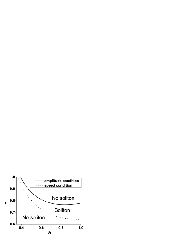
Figure 1: Graphical representation of (74) (dashed line) and (75) (solid line).

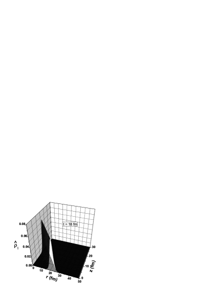
(a)

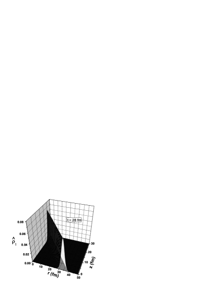
(b)

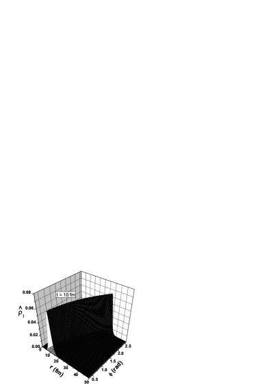
(c)

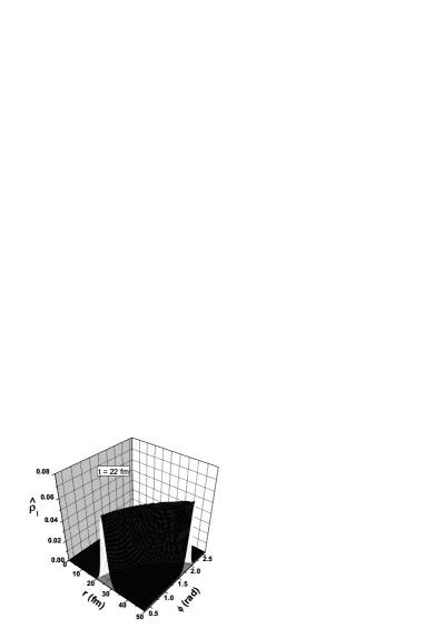
(d)

Figure 2: Graphical representation of (71) for different times, increasing from the left to the right. Upper and lower plots are for different parameter choices (see text).

V.2.2 Cartesian coordinates

We perform the study of the existence condition for the solution (72), which must be real and therefore the constant $U-w$ must be positive. Again we have chosen $\rho_{0}=1$ $fm^{-3}$ , $g=1.15$ and $m_{G}=460$ MeV, which imply $c_{s}\simeq 0.64$. We also set ${\mathcal{C}}=0.5$ and extend the condition in Refs. kp2010 ; moslempp17 to ${\mathcal{A}}^{2}+{\mathcal{B}}^{2}+{\mathcal{C}}^{2}=1$ . As mentioned, $U>w$ and from (73):

$$U-{\mathcal{A}}{c_{s}}-{\frac{[1-{\mathcal{A}}^{2}-{(0.5)}^{2}]{c_{s}}}{2}}-{\frac{{(0.5)}^{2}{c_{s}}}{2}}>0$$ (76)

Again, $\hat{\rho_{1}}$ is a normalized perturbation, so the amplitude condition must hold:

$${\frac{3(U-w)}{{\mathcal{A}}\alpha}}=\frac{3}{{\mathcal{A}}\alpha}\left(U-{\mathcal{A}}{c_{s}}-{\frac{[1-{\mathcal{A}}^{2}-{(0.5)}^{2}]{c_{s}}}{2}}-{\frac{{(0.5)}^{2}{c_{s}}}{2}}\right)<1$$ (77)

Within the region (in the $U-{\mathcal{A}}$ plane) where the conditions (76) and (77) are simultaneously satisfied, (72) is well defined and we can have solitons as it can be seen in Fig. 3. Again, the stability analysis can be performed more rigorously with the introduction of the Sagdeev potential kp2010 ; moslempp17 , which also provides (76) by using ${\mathcal{A}}x+{\mathcal{B}}y+{\mathcal{C}}z-Ut$, to rewrite equation (50) as an energy balance equation. The requirements (76) and (77) are sufficient to provide a soliton propagation in the present case.

A simple example of soliton evolution is presented in Fig. 4. We show a plot of (72) with fixed $z=1$ fm, ${\mathcal{A}}=0.6$, ${\mathcal{B}}\cong 0.62$, $U=0.66$ and $y$ varying in the range $0\,\mbox{fm}\leq y\,\leq 50\,\mbox{fm}$. This choice of parameters satisfies the soliton conditions (76) and (77). The pulse is observed at four times: $t=30$ fm (Fig. 4(a)) to $t=120$ fm (Fig. 4(d)). From the figure we can see that the cartesian pulse expands outwards in the $x$ direction keeping its shape and form.

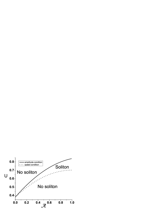
Figure 3: Graphical representation of (76) (dashed line) and (77) (solid line).

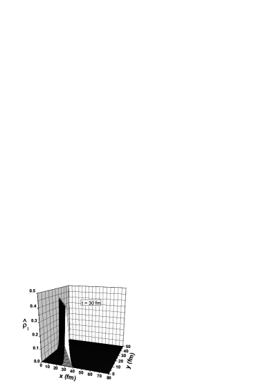
(a)

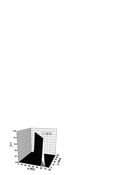
(b)

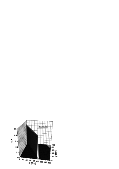
(c)

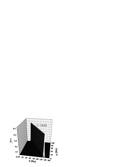
(d)

Figure 4: Graphical representation of (72) for different times, increasing from the left to the right and from upper to the lower. The plots are for the same parameter choices (see text).

VI Conclusions

We have described in detail how to obtain a KP equation in three dimensions in cylindrical and cartesian coordinates in the context of relativistic fluid dynamics of a cold quark gluon plasma. To this end, we have used the equation of state derived from QCD in nos2011 . The resulting nonlinear relativistic wave equations are for small perturbations in the baryon density.

For the cartesian KP the exact soliton solution is a supersonic bump keeping its shape without deformation. The cartesian KP contains some particular cases such as KdV and the breaking wave equation already encountered in our previous works nos2010 ; nos2011a . For the cylindrical KP (cKP) we also have an exact supersonic soliton solution which deforms slightly as time goes on due to the angular dependence in the phase.

We conclude that relativistic fluid dynamics supports nonlinear solitary waves even with the inclusion of transverse perturbations in cylindrical and cartesian geometry.

VII Appendix

In this appendix we start from the equations of relativistic hydrodynamics and, using the linearization approximation, we derive a wave equation for perturbations in the pressure. This equation has travelling wave solutions which represent acoustic waves. In the derivation presented here we follow closely Ref. hidro1 . The energy density and pressure for the relativistic fluid are written as:

$$\varepsilon(\vec{r},t)=\varepsilon_{0}+\delta\varepsilon(\vec{r},t)$$ (78)

and

$$p(\vec{r},t)=p_{0}+\delta p(\vec{r},t)$$ (79)

respectively. The uniform relativistic fluid is defined by $\varepsilon_{0}$ and $p_{0}$, while $\delta\varepsilon$ and $\delta p$ correspond to perturbations in this fluid. Energy-momentum conservation implies that:

$$\partial_{\mu}T^{\mu\nu}=0$$ (80)

where $T^{\mu\nu}$ is the energy-momentum tensor given by:

$$T^{\mu\nu}=(\varepsilon+p)u^{\mu}u^{\nu}-pg^{\mu\nu}$$ (81)

Linearization consists in keeping only first order terms such as $\delta\varepsilon$, $\delta P$ and $\vec{v}$ and neglect terms proportional to:

$${{v}}^{2},\hskip 5.69046ptv\delta\varepsilon,\hskip 5.69046ptv\delta P,\hskip 5.69046pt\vec{v}\cdot\vec{\nabla}v,\hskip 5.69046pt(\vec{v}\cdot\vec{\nabla})\vec{v}$$ (82)

and also neglect higher powers of these products or other combinations of them. Naturally we have:

$$\gamma={\frac{1}{\sqrt{1-v^{2}}}}\sim 1$$ (83)

From (80) we have:

$$u^{\mu}\partial_{\nu}[(\varepsilon+p)u^{\nu}]+(\varepsilon+p)u^{\nu}\partial_{\nu}u^{\mu}-\partial_{\nu}(pg^{\nu\mu})=0$$ (84)

The temporal component ($\mu=0$) of the above equation is given by:

$$\gamma\partial_{0}[(\varepsilon+p)\gamma]+\gamma\partial_{i}[(\varepsilon+p)u^{i}]+(\varepsilon+p)u^{0}\partial_{0}\gamma+(\varepsilon+p)u^{i}\partial_{i}\gamma-\partial_{0}p=0$$ (85)

which, after using (82) and (83), becomes:

$$\partial_{0}(\varepsilon+p)+\partial_{i}[(\varepsilon+p)v^{i}]-\partial_{0}p=0$$

or

$${\frac{\partial\varepsilon}{\partial t}}+\vec{\nabla}\cdot[(\varepsilon+p)\vec{v}]=0$$ (86)

For the $j$-th spatial component ($\mu=j$) in (84) we have:

$$u^{j}\partial_{0}[(\varepsilon+p)u^{0}]+u^{j}\partial_{i}[(\varepsilon+p)u^{i}]+(\varepsilon+p)u^{0}\partial_{0}u^{j}+(\varepsilon+p)u^{i}\partial_{i}u^{j}-\partial^{j}p=0$$

which, with the use of (82), becomes:

$${\frac{\partial}{\partial t}}[(\varepsilon+p)\vec{v}]+\vec{\nabla}p=0$$ (87)

Substituting the expansions (78) and (79) in (86) and (87) we find:

$${\frac{\partial}{\partial t}}[\varepsilon_{0}+\delta\varepsilon]+\vec{\nabla}\cdot[(\varepsilon_{0}+\delta\varepsilon+p_{0}+\delta p)\vec{v}]=0$$ (88)

and

$${\frac{\partial}{\partial t}}[(\varepsilon_{0}+\delta\varepsilon+p_{0}+\delta p)\vec{v}]+\vec{\nabla}[p_{0}+\delta p]=0$$ (89)

Using the linearization (82) and (83) in (88) and (89) they become:

$${\frac{\partial(\delta\varepsilon)}{\partial t}}+(\varepsilon_{0}+p_{0})\vec{\nabla}\cdot\vec{v}=0$$ (90)

and

$$(\varepsilon_{0}+p_{0}){\frac{\partial\vec{v}}{\partial t}}+\vec{\nabla}(\delta p)=0$$ (91)

Equation (90) expresses energy conservation and equation (91) is Newton’s second law. Integrating (91) with respect to the time and setting the integration constant to zero we find:

$$\vec{v}=-{\frac{1}{(\varepsilon_{0}+p_{0})}}\int{\vec{\nabla}(\delta p)}dt$$ (92)

which inserted in (90) yields:

$${\frac{\partial(\delta\varepsilon)}{\partial t}}-\int\vec{\nabla}^{2}(\delta p)dt=0$$ (93)

Performing the time derivative we obtain:

$${\frac{\partial^{2}(\delta\varepsilon)}{\partial t^{2}}}-\vec{\nabla}^{2}(\delta p)=0$$ (94)

Assuming that

$$\delta\varepsilon={\frac{\partial\varepsilon}{\partial p}}\delta p$$ (95)

with $\partial\varepsilon/\partial p$ being a constant, we have (94) rewritten as:

$${\frac{\partial\varepsilon}{\partial p}}{\frac{\partial^{2}(\delta p)}{\partial t^{2}}}-\vec{\nabla}^{2}(\delta p)=0$$ (96)

The above equation is a wave equation from where we can identify the velocity of propagation as:

$$c_{s}=\bigg{(}{\frac{\partial p}{\partial\varepsilon}}\bigg{)}^{1/2}$$ (97)

where $c_{s}$ is the speed of sound. Equation (96) can then be finally written as:

$$\vec{\nabla}^{2}(\delta p)-{\frac{1}{{c_{s}}^{2}}}{\frac{\partial^{2}(\delta p)}{\partial t^{2}}}=0$$ (98)

which describes the propagation of a pressure wave in the fluid.

The derivation presented above shows that the existence of sound waves in a relativistic perfect fluid depends only on the equation of state $p=p(\varepsilon)$. In particular, these formulas show that we can have acoustic waves in a medium made of massless particles. As a simple example, let us consider the equation of state given by (4) and (5) in the case where we have no gluons ($g=0$) and only massless quarks. In this case (4) and (5) reduce to:

$$\varepsilon=\mathcal{B}_{QCD}+3{\frac{\gamma_{Q}}{2{\pi}^{2}}}{\frac{{k_{F}}^{4}}{4}}$$ (99)

and

$$p=-\mathcal{B}_{QCD}+{\frac{\gamma_{Q}}{2{\pi}^{2}}}{\frac{{k_{F}}^{4}}{4}}$$ (100)

which can be combined to give:

$$p={\frac{1}{3}}\varepsilon-{\frac{4}{3}}\mathcal{B}_{QCD}$$ (101)

with the speed of sound $c_{s}$ given by (97):

$${c_{s}}^{2}={\frac{\partial p}{\partial\varepsilon}}={\frac{1}{3}}$$ (102)

- (1) “An Introduction to Quantum Field Theory”, M. Peskin and D. Schroeder, Addison-Wesley Publishing Company, (1995); “Quarks and Leptons: an Introductory Course in Modern Particle Physics”, F. Halzen and A.D. Martin, John Wiley and Sons, (1984); “Introduction to Elementary Particles”, D. Griffiths, John Wiley and Sons, (1987).
- (2) “Foundations of Quantum Chromodynamics”, T. Muta, World Scientific, (1987).
- (3) B. Betz, J. Noronha, G. Torrieri, M. Gyulassy and D. H. Rischke, Phys. Rev. Lett. 105, 222301 (2010) and references therein.
- (4) P. Staig and E. Shuryak, Phys. Rev. C 84, 044912 (2011); J. Casalderrey-Solana, E. V. Shuryak and D. Teaney, hep-ph/0602183.
- (5) For a recent review and a historical account see: H. Leblond, J. Phys. B: At. Mol. Opt. Phys. 41, 043001 (2008).
- (6) D. A. Fogaça, L. G. Ferreira Filho and F. S. Navarra, Phys. Rev. D 84, 054011 (2011).
- (7) B. B. Kadomtsev and V. I. Petviashivili, Sov. Phys. Dokl. 15, 539 (1970).
- (8) H. Washimi and T. Taniuti, Phys. Rev. Lett. 17, 996 (1966).
- (9) G. C. Das and K. M. Sen, Chaos, Solitons & Fractals, 3, 551 (1993).
- (10) Wen-shan Duan, Chaos, Solitons & Fractals, 14, 503 (2002).
- (11) Ju-Kui Xue, Phys. Plasmas 10, 3430 (2003).
- (12) S. K. El-Labany, Waleed M. Moslem, W. F. El-Taibany and M. Mahmoud, Physica Scripta 70, 317 (2004).
- (13) Mai-mai Lin and Wen-shan Duan, Chaos, Solitons & Fractals, 23, 929 (2005).
- (14) Yue-yue Wang and Jie-fang Zhang, Phys. Lett. A 352, 155 (2006).
- (15) Yunliang et al. , Phys. Lett. A 355, 386 (2006).
- (16) Yunliang Wang, Zhongxiang Zhou et al. , Phys. Plasmas 13, 052307 (2006).
- (17) A. Mushtaq, Phys. Plasmas 14, 113701 (2007).
- (18) Yue-yue Wang and Jie-fang Zhang, Phys. Lett. A 372, 3707 (2008).
- (19) Guang-jun He, Wen-shan Duan and Duo-xiang Tian, Phys. Plasmas 15, 043702 (2008).
- (20) W.M. Moslem, U.M. Abdelsalam, R. Sabry, E.F.El-Shamy and S.K. El-Labany, J. Plasma Phys. 76, 453 (2010).
- (21) W. M. Moslem, R. Sabry,and P. K. Shukla, Physics of Plasmas 17, 032305 (2010);
- (22) S. Weinberg,“Gravitation and Cosmology”, New York: Wiley, 1972.
- (23) L. Landau and E. Lifchitz, “Fluid Mechanics”, Pergamon Press, Oxford, (1987).
- (24) D. A. Fogaça and F. S. Navarra, Phys. Lett. B 700, 236 (2011).
- (25) D.A. Fogaça and F.S. Navarra, Phys. Lett. B 639, 629 (2006).
- (26) D.A. Fogaça and F.S. Navarra, Phys. Lett. B 645, 408 (2007).
- (27) D.A. Fogaça and F.S. Navarra, Nucl. Phys. A 790, 619c (2007); Int. J. Mod. Phys. E 16, 3019 (2007).
- (28) D.A. Fogaça, L. G. Ferreira Filho and F.S. Navarra, Nucl. Phys. A 819, 150 (2009).
- (29) D. A. Fogaça, L. G. Ferreira Filho and F. S. Navarra, Phys. Rev. C 81, 055211 (2010).
- (30) G. N. Fowler, S. Raha, N. Stelte and R.M. Weiner, Phys. Lett. B 115, 286 (1982); S. Raha, K. Wehrberger and R.M. Weiner, Nucl. Phys. A 433, 427 (1984); E.F. Hefter, S. Raha and R.M. Weiner, Phys. Rev. C 32, 2201 (1985).
- (31) A.Y. Abul-Magd, I. El-Taher and F.M. Khaliel, Phys. Rev. C 45, 448 (1992).
- (32) D. A. Fogaça and F. S. Navarra, Journal of Physics: Conference Series 316, 012029 (2011).
- (33) T. Taniuti, Wave Motion 12, 373 (1990).
- (34) D. A. Fogaça, F.S. Navarra and L. G. Ferreira Filho, Nucl. Phys. A 887, 22 (2012).
- (35) M. J. Ablowitz and H. Segur, “Solitons and the Inverse Scattering Transform”, SIAM (Studies in Applied Mathematics), 1981;
- (36) S. Novikov, S. V. Manakov , L. P. Pitaevskii and V. E. Zakharov, “Theory of solitons: the inverse scattering method”, New York and London, 1984.
- (37) B. A Dubrovin, Russ. Math. Surv. 36, 11 (1981).
- (38) Biswajit Sahu, Phys. Plasmas 18, 062308 (2011).
- (39) Kenneth L. Jones, Internat. J. Math. & Math. Sci. 24, No. 6, 379 (2000).
- (40) Gino Biondini, Phys. Rev. Lett. 99, 064103 (2007).
- (41) J.Y. Ollitrault, Eur. J. Phys. 29, 275 (2008); arXiv:0708.2433 [nucl-th].