Accelerating Atomic Orbital-based Electronic Structure Calculation via Pole Expansion and Selected Inversion

Abstract

We describe how to apply the recently developed pole expansion and selected inversion (PEXSI) technique to Kohn-Sham density function theory (DFT) electronic structure calculations that are based on atomic orbital discretization. We give analytic expressions for evaluating the charge density, the total energy, the Helmholtz free energy and the atomic forces (including both the Hellman-Feynman force and the Pulay force) without using the eigenvalues and eigenvectors of the Kohn-Sham Hamiltonian. We also show how to update the chemical potential without using Kohn-Sham eigenvalues. The advantage of using PEXSI is that it has a much lower computational complexity than that associated with the matrix diagonalization procedure. We demonstrate the performance gain by comparing the timing of PEXSI with that of diagonalization on insulating and metallic nanotubes. For these quasi-1D systems, the complexity of PEXSI is linear with respect to the number of atoms. This linear scaling can be observed in our computational experiments when the number of atoms in a nanotube is larger than a few hundreds. Both the wall clock time and the memory requirement of PEXSI is modest. This makes it even possible to perform Kohn-Sham DFT calculations for 10,000-atom nanotubes with a sequential implementation of the selected inversion algorithm. We also perform an accurate geometry optimization calculation on a truncated (8,0) boron-nitride nanotube system containing 1024 atoms. Numerical results indicate that the use of PEXSI does not lead to loss of accuracy required in a practical DFT calculation.

I Introduction

Electronic structure calculations based on solving the Kohn-Sham density functional theory (KSDFT) play an important role in the analysis of electronic, structural and optical properties of molecules, solids and other nano structures. The efficiency of such a calculation depends largely on the computational cost associated with the evaluation of the electron charge density for a given potential within a self-consistent field (SCF) iteration. The most straightforward way to perform such an evaluation is to partially diagonalize the Kohn-Sham Hamiltonian by computing a set of eigenvectors corresponding to the algebraically smallest eigenvalues of the Hamiltonian. The complexity of this approach is $\mathcal{O}(N_{e}^{3})$, where $N_{e}$ is the number of electrons in the atomistic system of interest. As the number of atoms or electrons in the system increases, the cost of diagonalization becomes prohibitively expensive.

Linear scaling algorithms (or $\mathcal{O}(N_{e})$ scaling methods, see for example Bowler et al. (2002); Fattebert and Bernholc (2000); Hine et al. (2009); Yang (1991); Li et al. (1993); McWeeny (1960), and review articles Goedecker (1999); Bowler and Miyazaki (2012)) are attractive alternatives for solving KSDFT. The traditional linear scaling methods use the nearsightedness principle, which asserts that the density perturbation induced by a local change in the external potential decays exponentially away from where the perturbation is applied. Consequently, the off-diagonal elements of the density matrix decay exponentially away from the diagonal Kohn (1996); Prodan and Kohn (2005). Strictly speaking, the nearsightedness property is valid for insulating systems but not for metallic systems.

In order to design a fast algorithm that is accurate for both insulating and metallic systems, we use an equivalent formulation of KSDFT, in which the charge density is evaluated as the diagonal of the Fermi-Dirac function evaluated at a fixed Kohn-Sham Hamiltonian. By approximating the Fermi-Dirac function through a pole expansion technique Lin et al. (2009a), we can reduce the problem of computing the charge density to that of computing the diagonal of the inverses of a number of shifted Kohn-Sham Hamiltonians. This approach was pursued by a number of researchers in the past. The cost of this approach depends on the number of poles required to expand the Fermi-Dirac function and the cost for computing the diagonal of the inverse of a shifted Kohn-Sham Hamiltonian.

The recent work by Lin et al. Lin et al. (2009a) provides an accurate and efficient pole-expansion scheme for approximating the Fermi-Dirac function. The number of poles required in this approach is proportional to $\log(\beta\Delta E)$, where $\beta$ is proportional to the inverse of the temperature, and $\Delta E$ is the spectral width of the Kohn-Sham Hamiltonian. (i.e. the difference between the largest and the smallest eigenvalues). This number of expansion terms, or the pole count here is significantly lower than those given in the previous approaches Baroni and Giannozzi (1992); Goedecker (1993); Ozaki (2007); Ceriotti et al. (2008); Ozaki (2010). When temperature decreases, $\beta$ becomes large. The favorable scaling of the pole expansion allows us to treat both insulating and metallic systems efficiently at room temperature or even lower temperature.

Furthermore, an efficient selected inversion algorithm for computing the inverse of the diagonal of a shifted Kohn-Sham Hamiltonian without computing the full inverse of the Hamiltonian has been developed  Lin et al. (2009b, 2011a, 2011b). The idea of using the inverse of shifted Hamiltonian operator (Green’s function) for reducing the complexity of Kohn-Sham density functional theory has also been pursued in other recent works Varga (2010); Ozaki (2010). In the selected inversion method, the complexity of this algorithm is $\mathcal{O}(N_{e})$ for quasi-1D systems such as nanorods, nanotubes and nanowires, $\mathcal{O}(N_{e}^{3/2})$ for quasi-2D systems such as graphene and surfaces, and $\mathcal{O}(N_{e}^{2})$ for 3D bulk systems. In exact arithmetic, the selected inversion algorithm gives the exact diagonal of the inverse, i.e., the algorithm does not rely on any type of localization or truncation scheme. For insulating systems, the use of localization and truncation can be combined with selected inversion to reduce the complexity of the algorithm further to $\mathcal{O}(N_{e})$ even for general 3D systems.

In the previous work Lin et al. (2011a, b), we used the pole expansion and selected inversion (PEXSI) technique to solve the Kohn-Sham problem discretized by a finite difference scheme. However, it is worth pointing out that PEXSI is a general technique that is not limited to discretized problems obtained from finite difference. In particular, it can be readily applied to discretized Kohn-Sham problems obtained from any localized basis expansion technique. In this paper, we describe how PEXSI can be used to speed up the solution of a discretized Kohn-Sham problem obtained from an atomic orbital basis expansion. We show that electron charge density, total energy, Helmholtz free energy and atomic forces can all be efficiently calculated by using PEXSI.

We demonstrate the performance gain we can achieve by comparing PEXSI with the LAPACK diagonalization subroutine dsygv on two types of nanotubes. We show that by using the PEXSI technique, it is possible to perform electronic structure calculations accurately for a nanotube that contains 10,000 atoms with a sequential implementation of the selected inversion algorithm within a reasonable amount of time. This is not possible with the sequential LAPACK subroutine. For this example, PEXSI exhibits linear scaling when the system size exceeds a few hundred atoms.

This paper is organized as follows. In section II, we show how the PEXSI technique previously developed Lin et al. (2009a, b, 2011a, 2011b) can be extended to solve discretized Kohn-Sham problems obtained from an atomic orbital expansion scheme. In particular, we will show how charge density, total energy, free energy and force can be calculated in this formalism. We will also discuss how to update the chemical potential. In section III, we report the performance of PEXSI on two quasi-1D test problems.

Throughout the paper, we use $\mathfrak{Im}(A)$ to denote the imaginary part of a complex matrix $A$. A properly defined inner product between two functions $f$ and $g$ is sometimes denoted by $\langle f|g\rangle$. The diagonal of a matrix $A$ is sometimes denoted by $\mbox{diag}(A)$. We use $\hat{H}(x,x^{\prime})$ to denote the Hamiltonian operator, and $H,S$ to denote the discretized Hamiltonian matrix and the corresponding overlap matrix obtained from a basis set $\Phi$. Similarly $\hat{\gamma}(x,x^{\prime})$ denotes the single particle density matrix operator, and the corresponding electron density is denoted by $\hat{\rho}(x)$. The matrix $\Gamma$ denotes the single particle density matrix represented under a basis set $\Phi$. It will be used to define the electron density $\hat{\rho}$ and the total energy $E_{\mathrm{tot}}$. In a finite temperature ab initio molecular dynamics simulation, we also need the Helmholtz free energy $\mathcal{F}_{\mathrm{tot}}$, and the atomic forces on the nuclei $\{F_{I}\}$. To compute these quantities without using Kohn-Sham eigenvalues and Kohn-Sham orbitals, we need the free energy density matrix $\Gamma^{\mathcal{F}}$ and the energy density matrix $\Gamma^{E}$. In PEXSI, these matrices are approximated by a finite $P$-term pole expansion, denoted by $\Gamma_{P},\Gamma^{\mathcal{F}}_{P},\Gamma^{E}_{P}$ respectively. However, to simplify notation, we will drop the subscript $P$ and simply use $\Gamma,\Gamma^{\mathcal{F}},\Gamma^{E}$ to denote the approximated matrices unless otherwise noted.

II Theory

The ground-state electron charge density $\hat{\rho}(x)$ of an atomistic system can be obtained from the self-consistent solution to the Kohn-Sham equations

$$\hat{H}\left[\hat{\rho}(x)\right]\psi_{i}(x)=\psi_{i}(x)\varepsilon_{i},$$ (1)

where $\hat{H}$ is the Kohn-Sham Hamiltonian that depends on $\hat{\rho}(x)$, $\{\psi_{i}(x)\}$ are the Kohn-Sham orbitals that satisfy the orthonormality constraints

$$\int\psi^{\ast}_{i}(x)\psi_{j}(x)dx=\delta_{ij},$$ (2)

and the eigenvalue $\varepsilon_{i}$ is often known as the $i$th Kohn-Sham energy level. Using the Kohn-Sham orbitals, we can define the charge density by

$$\hat{\rho}(x)=\sum_{i}^{\infty}|\psi_{i}(x)|^{2}f_{i},\ \ i=1,2,...,\infty,$$ (3)

with occupation numbers $0\leq f_{i}\leq 2$, $i=1,2,...\infty$. The occupation numbers in (3) can be chosen according to the Fermi-Dirac distribution function

$$f_{i}=f_{\beta}(\varepsilon_{i}-\mu)=\frac{2}{1+e^{\beta(\varepsilon_{i}-\mu)}},$$ (4)

where $\mu$ is the chemical potential chosen to ensure that

$$\int\hat{\rho}(x)dx=N_{e},$$ (5)

and $\beta$ is the inverse of the temperature, i.e., $\beta=1/(k_{B}T)$ with $k_{B}$ being the Boltzmann constant.

Note that $\hat{\rho}(x)$ is simply the diagonal of the single particle density matrix defined by

$$\hat{\gamma}(x,x^{\prime})=\sum_{i=1}^{\infty}\psi_{i}(x)f_{\beta}(\varepsilon_{i}-\mu)\psi_{i}^{\ast}(x^{\prime}),$$ (6)

and the charge sum rule in (5) can be expressed alternatively by

$$\mbox{Tr}\left[\hat{\gamma}(x,x^{\prime})\right]=N_{e},$$ (7)

where Tr denotes the trace of an operator.

It follows from (1) and (6) that the electron density $\hat{\rho}(x)$ is a fixed point of the Kohn-Sham map defined by

$$\hat{\rho}(x)=\operatorname{diag}\left(f_{\beta}(\hat{H}[\hat{\rho}(x)]-\mu\delta(x,x^{\prime}))\right),$$ (8)

where $\mu$ is chosen to satisfy (7). The most widely used algorithm for finding the solution to (7) and (8) is a Broyden type of quasi-Newton algorithm. In the physics literature, this is often referred to as the self-consistent field (SCF) iteration. The most time consuming part of this algorithm is the evaluation of $\hat{\rho}(x)=\hat{\gamma}(x,x)$ in (8).

II.1 Basis expansion by nonorthogonal basis functions

An infinite-dimensional Kohn-Sham problem can be discretized in a number of ways (e.g., planewave expansion, finite difference, finite element etc.). In this paper, we focus on a discretization scheme in which a Kohn-Sham orbital $\psi_{i}$ is expanded by a linear combination of a finite number of basis functions $\{\varphi_{j}\}$, i.e.,

$$\psi_{i}(x)=\sum_{j=1}^{N}\varphi_{j}(x)c_{ji}.$$ (9)

We should note that the total number of basis functions $N$ is generally proportional to the number of electrons $N_{e}$ or atoms in the system to be studied. These basis functions $\{\varphi_{j}\}$ can be constructed to have local nonzero support. But they may not necessarily be orthonormal to each other. Examples of these basis functions include Gaussian type orbitals Frisch et al. (1984); VandeVondele et al. (2005) and local atomic orbitals Junquera et al. (2001); Chen et al. (2010, 2011); Kenny et al. (2000); Ozaki (2003); Blum et al. (2009), adaptive curvilinear coordinates Tsuchida and Tsukada (1998), optimized nonorthogonal orbitals Bowler et al. (2002); Fattebert and Bernholc (2000); Hine et al. (2009) and adaptive local basis functions Lin et al. (2012). In numerical examples presented in section III, we use a set of nonorthogonal local atomic orbitals.

Substituting (9) into (1) yields a generalized eigenvalue problem

$$HC=SC\Xi,$$ (10)

where $C$ is an $N\times N$ matrix with $c_{ij}$ being its $(i,j)$th entry, $\Xi$ is a diagonal matrix with $\varepsilon_{i}$ on its diagonal, $S_{ij}=\langle\varphi_{i}|\varphi_{j}\rangle$, and $H_{ij}=\langle\varphi_{i}\lvert\hat{H}\rvert\varphi_{j}\rangle$. For orthogonal basis functions, the overlap matrix $S$ is an identity matrix, and Eq. (10) reduces to a standard eigenvalue problem. When local atomic orbitals are used as the basis, $S$ is generally not an identity matrix, but both $H$ and $S$ are sparse.

Without loss of generality, we assume the basis functions and the Kohn-Sham orbitals to be real in the following discussion. Let $\Psi=[\psi_{1},\cdots,\psi_{N}]$ and $\Phi=[\varphi_{1},\cdots,\varphi_{N}]$, Then Eq. (9) can be written in a compact form

$$\Psi=\Phi C.$$ (11)

Consequently, the single particle density matrix (6) becomes Fattebert and Bernholc (2000)

$$\begin{split}\hat{\gamma}(x,x^{\prime})&=\Psi(x)f_{\beta}(\Xi-\mu)\Psi^{T}(x^{\prime})\\ &=\Phi(x)Cf_{\beta}(\Xi-\mu)C^{T}\Phi^{T}(x^{\prime}).\end{split}$$ (12)

II.2 Pole expansion and selected inversion for nonorthogonal basis functions

The most straightforward way to evaluate $\hat{\gamma}(x,x^{\prime})$ is to follow the right hand side of (12), which requires solving the generalized eigenvalue problem (10). The computational complexity of this approach is $\mathcal{O}(N^{3})$. This approach becomes prohibitively expensive when the number of electrons or atoms in the system increases.

An alternative way to evaluate $\hat{\gamma}(x,x^{\prime})$, which circumvents the cubic scaling of the diagonalization process, is to approximate $\hat{\gamma}(x,x^{\prime})$ by a Fermi operator expansion (FOE) method Goedecker (1993). In an FOE scheme, the function $f_{\beta}(\Xi-\mu)$ is approximated by a linear combination of a number of simpler functions, each of which can be evaluated directly without diagonalizing the matrix pencil $(H,S)$. A variety of FOE schemes have been developed. They include polynomial expansion Goedecker (1993), rational expansion Lin et al. (2009a); Baroni and Giannozzi (1992); Ozaki (2007), and a hybrid scheme in which both polynomials and rational functions are used Ceriotti et al. (2008); Lin et al. (2009c). In all these schemes, the number of simple functions used in the expansion is asymptotically determined by $\beta\Delta E$, where $\Delta E=\max_{i=1}^{N}\left\lvert\varepsilon_{i}-\mu\right\rvert$ is the spectrum width for the discrete problem. An upper bound of $\Delta E$ can be obtained inexpensively by a very small number of Lanczos steps Lanczos (1950).

While most of the FOE schemes require as many as $\mathcal{O}(\beta\Delta E)$ or $\mathcal{O}(\sqrt{\beta\Delta E})$ terms of simple functions, the recently developed pole expansion Lin et al. (2009a) is particularly promising since it requires only $\mathcal{O}(\log\beta\Delta E)$ terms of simple rational functions. The favorable scaling of the pole expansion allows us to treat both insulating and metallic systems efficiently at room or even lower temperature. The pole expansion has the analytic expression

$$f_{\beta}(\varepsilon-\mu)\approx\mathfrak{Im}\sum_{l=1}^{P}\frac{\omega^{\rho}_{l}}{\varepsilon-(z_{l}+\mu)},$$ (13)

where

$$w_{l}^{\rho}=\frac{4K\sqrt{mM}}{\pi kP}\frac{\mathrm{cn}(t_{l})\mathrm{dn}(t_{l})}{z_{l}(k^{-1}-\mathrm{sn}(t_{l}))^{2}}f_{\beta}(z_{l}),$$ (14)

with $m=\frac{\pi^{2}}{\beta^{2}},M=\Delta E^{2}+\frac{\pi^{2}}{\beta^{2}},k=\frac{\sqrt{M/m}-1}{\sqrt{M/m}+1}$. The functions $\mathrm{cn},\mathrm{dn},\mathrm{sn}$ are Jacobi elliptic functions, and $K,\{z_{l}\},\{t_{l}\}$ are chosen carefully and computed from analytic expressions. We refer the readers to Ref. Lin et al., 2009a for more detailed explanations. In the following discussions, we will also refer to $\{z_{l}\}$ as the complex shifts or poles, and refer to $\{\omega^{\rho}_{l}\}$ as the complex weights. The complex shifts and weights are determined only by $\beta,\Delta E$ and the number of poles $P$. All quantities in the pole expansion are known explicitly and their calculation takes negligible amount of time. The construction of pole expansion is based on the observation that the non-analytic part of the Fermi-Dirac function lies only on the imaginary axis within $\left[\frac{i\pi}{\beta},+i\infty\right]\bigcup\left[-i\infty,-\frac{i\pi}{\beta}\right]$. A dumbbell-shaped Cauchy contour (see Fig. 1) is carefully chosen and discretized to circle the eigenvalues $\{\varepsilon_{i}\}$ on the real axis, while avoiding the intersection with the non-analytic region. The pole expansion does not require a band gap between the occupied and unoccupied states. Therefore, it is applicable to both insulating and metallic systems. Furthermore, the construction of the pole expansion relies only on the analytical structure of the Fermi-Dirac function rather than its detailed shape. This is a key property that is crucial for constructing pole expansions for other functions, including the free energy density matrix and the energy density matrix which are discussed in section II.3 for the purpose of computing Helmholtz free energy and atomic forces (including both the Hellman-Feynman force and the Pulay force). In such case, one only needs to substitute $f_{\beta}$ in the weight function in Eq. (14) by the corresponding function that shares the same analytic structure as the Fermi-Dirac function $f_{\beta}$.

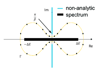
Figure 1: (color online) A schematic view of the placement of poles used in a pole expansion approximation of $f_{\beta}(z)$. The thick black line on the real axis indicates the range of $\varepsilon_{i}-\mu$, and the thin blue line on the imaginary axis indicates the non-analytic part of $f_{\beta}(z)$. The yellow dumbbell shaped contour is chosen to exclude the non-analytic part of the complex plane. Each block dot on the contour corresponds to a pole used in the pole expansion approximation.

Following the derivation in the appendix, we can use (13) to approximate the single particle density matrix $\hat{\gamma}$ by its $P$-term pole expansion, denoted by $\hat{\gamma}_{P}$ as

$$\begin{split}\hat{\gamma}_{P}(x,x^{\prime})&=\Phi(x)\mathfrak{Im}\left(\sum_{l=1}^{P}\frac{\omega^{\rho}_{l}}{H-(z_{l}+\mu)S}\right)\Phi^{T}(x^{\prime})\\ &\equiv\Phi(x)\Gamma\Phi^{T}(x^{\prime}).\end{split}$$ (15)

In the above expression, $\Gamma$ is an $N\times N$ matrix represented in terms of the atomic orbitals $\Phi$. To simplify our notation, we will drop the subscript $P$ from the $P$-term pole expansion approximation of single particle density matrix $\hat{\gamma}$ unless otherwise noted. Similar treatment will be made for the electron density $\hat{\rho}$, the total energy $E_{\mathrm{tot}}$, the Helmholtz free energy $\mathcal{F}_{\mathrm{tot}}$, and the atomic force on the $I$-th nuclei $F_{I}$. Using Eq. (15), we can evaluate the electron density in the real space as the diagonal elements of $\hat{\gamma}$, i.e.,

$$\hat{\rho}(x)=\Phi(x)\Gamma\Phi^{T}(x)=\sum_{ij}\Gamma_{ij}\varphi_{j}(x)\varphi_{i}(x).$$ (16)

We assume that each basis function $\varphi_{i}(x)$ is compactly supported in the real space. In order to evaluate $\hat{\rho}(x)$ for any particular $x$, we only need $\Gamma_{ij}$ such that $\varphi_{j}(x)\varphi_{i}(x)\neq 0$, or $S_{ij}\neq 0$. This set of $\Gamma_{ij}$’s is a subset of $\{\Gamma_{ij}|H_{ij}\neq 0\}$. To obtain these selected elements, we need to compute the corresponding elements of $(H-(z_{l}+\mu)S)^{-1}$ for all $z_{l}$.

The recently developed selected inversion method Lin et al. (2009b, 2011a, 2011b) provides an efficient way of computing the selected elements of an inverse matrix. For a symmetric matrix of the form $A=H-zS$, the selected inversion algorithm first constructs an $LDL^{T}$ factorization of $A$, where $L$ is a block lower diagonal matrix called the Cholesky factor, and $D$ is a block diagonal matrix. In the second step, the selected inversion algorithm computes all the elements $A^{-1}_{ij}$ such that $L_{ij}\neq 0$. Since $L_{ij}\neq 0$ implies that $H_{ij}\neq 0$, all the selected elements of $A^{-1}$ required in (16) are computed. As a result, the computational scaling of the selected inversion algorithm is only proportional to the number of nonzero elements in the Cholesky factor $L$. In particular, the selected inversion algorithm has a complexity of $\mathcal{O}(N)$ for quasi-1D systems, $\mathcal{O}(N^{1.5})$ for quasi-2D systems, and $\mathcal{O}(N^{2})$ for 3D bulk systems. The selected inversion algorithm achieves universal improvement over the diagonalization method for systems of all dimensions. It should be noted that selected inversion algorithm is an exact method for computing selected elements of $A^{-1}$ if exact arithmetic is to be employed, and in practice the only source of error is the roundoff error. In particular, the selected inversion algorithm does not rely on any localization property of $A^{-1}$. However, it can be combined with localization properties of insulating systems to further reduce the computational cost. We will pursue this approach in future work. We also remark that the PEXSI technique can be applied whenever $H$ and $S$ are sparse matrices. However, since the selected inversion method relies on an $LDL^{T}$ factorization of $H-zS$, the preconstant of the selected inversion method asymptotically scales cubically with respect to the number of basis functions per atom. The number of basis functions or degrees of freedom per atom associated with the finite difference method Chelikowsky et al. (1994) and the finite element method Tsuchida and Tsukada (1995) is usually much larger than that associated with methods based on contracted basis functions such as local atomic orbitals. Therefore the finite difference method and the finite element method do not benefit as much from the PEXSI technique as methods that are based on local atomic orbitals.

II.3 Total energy, Helmholtz free energy and atomic force evaluation

In addition to reducing the computational complexity of the charge density calculation in each SCF iteration, the PEXSI technique can also be used to compute the total energy, the Helmholtz free energy as well as the atomic forces (including both the Hellman-Feynman force and the Pulay force) efficiently without diagonalizing the Kohn-Sham Hamiltonian.

It is well known that Eqs. (1)- (5) can be derived as the first order necessary condition for minimizing the Mermin free energy Mermin (1965); Soler et al. (2002); Kresse and Furthmüller (1996); Weinert and Davenport (1992); Wentzcovitch et al. (1992)

$$\begin{split}\mathcal{F}_{\mathrm{tot}}\left[\{\psi_{i}\},\{f_{i}\}\right]=&E_{\mathrm{tot}}\left[\{\psi_{i}\},\{f_{i}\}\right]-TS\left[\{f_{i}\}\right],\end{split}$$ (17)

under the constraints (2) and $\sum_{i=1}^{\infty}f_{i}=N_{e}$, where

$$\begin{split}E_{\mathrm{tot}}\left[\{\psi_{i}\},\{f_{i}\}\right]=&\sum_{i=1}^{\infty}f_{i}\varepsilon_{i}-\frac{1}{2}\iint\frac{\hat{\rho}(x)\hat{\rho}(y)}{\left\lvert x-y\right\rvert}\,\mathrm{d}x\,\mathrm{d}y\\ &+E_{{\mathrm{xc}}}[\hat{\rho}]-\int V_{{\mathrm{xc}}}[\hat{\rho}](x)\hat{\rho}(x)\,\mathrm{d}x\end{split}$$ (18)

is called the internal energy or the total energy,

$$S\left[\{f_{i}\}\right]=-2k_{B}\sum_{i=1}^{\infty}\left(\tilde{f}_{i}\log\tilde{f}_{i}+(1-\tilde{f}_{i})\log(1-\tilde{f}_{i})\right)$$ (19)

is the entropy due to fractional occupation where $\tilde{f_{i}}=f_{i}/2$ is used so that $0\leq\tilde{f}_{i}\leq 1$. The chemical potential $\mu$ in (4) is simply the Lagrange multiplier associated with occupation number constraint $\sum_{i=1}^{\infty}f_{i}=N_{e}$.

Furthermore, it is the derivative of the Mermin free energy (rather than the total energy) with respect to the atomic positions that give rise to the correct force in ab initio molecular dynamics simulation Soler et al. (2002); Kresse and Furthmüller (1996); Weinert and Davenport (1992); Wentzcovitch et al. (1992).

The evaluation of the Mermin free energy functional $\mathcal{F}_{\mathrm{tot}}$ requires the explicit knowledge of the Kohn-Sham eigenvalues $\{\varepsilon_{i}\}$ which are not available in the PEXSI scheme. However, it has been shown in Ref. Alavi et al., 1994 that the Mermin free energy can be equivalently computed in the form of the following Helmholtz free energy, which does not contain the Kohn-Sham eigenvalues explicitly

$$\begin{split}\mathcal{F}_{\mathrm{tot}}=&-2\beta^{-1}\operatorname{Tr}\ln(1+\exp(\beta(\mu-\Xi)))+\mu N_{e}\\ &-\frac{1}{2}\iint\frac{\hat{\rho}(x)\hat{\rho}(y)}{\left\lvert x-y\right\rvert}\,\mathrm{d}x\,\mathrm{d}y+E_{{\mathrm{xc}}}[\hat{\rho}]\\ &-\int V_{{\mathrm{xc}}}[\hat{\rho}](x)\hat{\rho}(x)\,\mathrm{d}x.\end{split}$$ (20)

Here we assume LDA Ceperley and Alder (1980) or GGA Becke (1988); Lee et al. (1988) exchange-correlation functional is used for the Kohn-Sham total energy expression. In section II.2 we have shown that the electron density $\hat{\rho}(x)$ can be computed in the PEXSI scheme. Therefore in Eq. (20), only the first term requires extra treatment. Note that the function

$$f^{\mathcal{F}}_{\beta}(\varepsilon-\mu)=-2\beta^{-1}\ln(1+\exp(\beta(\mu-\varepsilon)))$$ (21)

is different from the Fermi-Dirac function $f_{\beta}$ in Eq. (4). In fact $f^{\mathcal{F}}_{\beta}$ is directly related to the $f_{\beta}$ as

$$\left(f^{\mathcal{F}}_{\beta}\right)^{\prime}(z)=f_{\beta}(z).$$ (22)

Nonetheless $f^{\mathcal{F}}_{\beta}(z)$ is analytic everywhere in the complex plane, except for segments of the imaginary axis within $\left[\frac{i\pi}{\beta},+i\infty\right]\bigcup\left[-i\infty,-\frac{i\pi}{\beta}\right]$. In this sense, $f^{\mathcal{F}}_{\beta}$ shares the same analytic structure as that of the Fermi-Dirac function $f_{\beta}$. The pole expansion technique can be applied with the same choice of poles $\{z_{l}\}$ but different weights, denoted by $\{\omega_{l}^{\mathcal{F}}\}$, i.e.

$$f^{\mathcal{F}}_{\beta}(\varepsilon-\mu)\approx\mathfrak{Im}\sum_{l=1}^{P}\frac{\omega^{\mathcal{F}}_{l}}{\varepsilon-(z_{l}+\mu)}.$$ (23)

Following the derivation in the appendix, we can rewrite the Helmholtz free energy as

$$\begin{split}\mathcal{F}_{\mathrm{tot}}=&\operatorname{Tr}[\Gamma^{\mathcal{F}}S]+\mu N_{e}-\frac{1}{2}\iint\frac{\hat{\rho}(x)\hat{\rho}(y)}{\left\lvert x-y\right\rvert}\,\mathrm{d}x\,\mathrm{d}y\\ &+E_{{\mathrm{xc}}}[\hat{\rho}]-\int V_{{\mathrm{xc}}}[\hat{\rho}]\hat{\rho}(x)\,\mathrm{d}x,\end{split}$$ (24)

where the free energy density matrix $\Gamma^{\mathcal{F}}$ is given by

$$\Gamma^{\mathcal{F}}=\mathfrak{Im}\sum_{l=1}^{P}\frac{\omega^{\mathcal{F}}_{l}}{H-(z_{l}+\mu)S}.$$ (25)

Note that in the expression (24), the first term depends on the trace of the product of $\Gamma^{\mathcal{F}}$ and $S$. The computation of this term requires only the $(i,j)$th entry of $\Gamma^{\mathcal{F}}$ for $(i,j)$ satisfying $S_{ij}\neq 0$ or $H_{ij}\neq 0$. Since the poles $\{z_{l}\}$ are the same as those used for computing the electron density, the selected elements of $\Gamma^{\mathcal{F}}$ correspond to the same selected elements of $\left(H-(z_{l}+\mu)S\right)^{-1}$ used for the charge density calculation. Thus using them for computing $\mathcal{F}_{\mathrm{tot}}$ does not introduce additional complexity.

It is worth mentioning that the above formulation can be simplified for insulating systems with a relatively large band gap (even at zero temperature). In such cases, $f_{i}$ can be chosen to be $2$ for occupied states and $0$ for unoccupied states. Then the entropy term $S$ vanishes and $\mathcal{F}_{\mathrm{tot}}=E_{\mathrm{tot}}$. Furthermore, similar to the Helmholtz free energy, an alternative expression for $E_{\mathrm{tot}}$ is

$$\begin{split}E_{\mathrm{tot}}=&\operatorname{Tr}[\Gamma H]-\frac{1}{2}\iint\frac{\hat{\rho}(x)\hat{\rho}(y)}{\left\lvert x-y\right\rvert}\,\mathrm{d}x\,\mathrm{d}y\\ &+E_{{\mathrm{xc}}}[\hat{\rho}]-\int V_{{\mathrm{xc}}}[\hat{\rho}](x)\hat{\rho}(x)\,\mathrm{d}x,\end{split}$$ (26)

where $\Gamma$ is the density matrix defined in (6). Note that in this expression, the first term depends on the trace of the product of $\Gamma$ and $H$. The computation of this term requires only the $(i,j)$th entry of $\Gamma$ for $(i,j)$ satisfying $H_{ij}\neq 0$. These entries are already available from the charge density calculation, thus using them for total energy evaluation does not introduce additional complexity.

To perform geometric optimization or ab initio molecular dynamics, we need to compute atomic forces associated with different atoms. Atomic force is the derivative of the free energy with respect to the position of an atom. For nonorthogonal atomic basis set, the force calculation is not trivial, and standard methods have established in Ref. Soler et al., 2002 to calculate the force. The calculation includes both the Hellman-Feynman force and the Pulay force Pulay (1969), where the Pulay force is induced by the change of basis functions with respect to atomic positions. Following the derivation in the appendix, we can express the atomic force associated with the $I$-th atom in a compact way as

$$F_{I}=-\frac{\partial\mathcal{F}_{\mathrm{tot}}}{\partial R_{I}}=-\operatorname{Tr}\left[\Gamma\frac{\partial H}{\partial R_{I}}\right]+\operatorname{Tr}\left[\Gamma^{E}\frac{\partial S}{\partial R_{I}}\right].$$ (27)

where $\Gamma^{E}$ is the energy density matrix defined by

$$\Gamma^{E}=C\Xi f_{\beta}(\Xi-\mu)C^{T}.$$ (28)

We remark that Eq. (27) itself is not new. We re-derive this formula in the appendix using linear algebra notation to make the manuscript more accessible to readers not familiar with this subject. The concept of the energy density matrix has been used before Sankey and Niklewski (1989); Soler et al. (2002), and the last term in Eq. (27) is also referred to as the “orthogonalization force” in the appendix of Ref. Soler et al., 2002, which takes into account the fact that eigenfunctions must be orthogonalized after atomic positions change.

To illustrate more clearly that both the Hellman-Feynman force and the Pulay force are taken into account correctly, let us look into the first term in Eq. (27),

$$\begin{split}\frac{\partial H_{ij}}{\partial R_{I}}&=\left\langle\frac{\partial\varphi_{i}}{\partial R_{I}},\hat{H}\varphi_{j}\right\rangle+\left\langle\varphi_{i},\frac{\partial{\hat{H}}}{\partial{R_{I}}}\varphi_{j}\right\rangle\\ &+\left\langle\varphi_{i},\hat{H}\frac{\partial\varphi_{j}}{\partial R_{I}}\right\rangle.\end{split}$$ (29)

The terms $\frac{\partial\varphi_{i}}{\partial R_{I}}$ are automatically included to reflect the change of the atom-centered basis functions with respect to atomic positions, which gives rise to the Pulay force. From a computational point of view, the terms in Eq. (29) that are related to the kinetic and non-local pseudopotential parts can be solved by efficient two center integrals techniques, while the terms related to local potential parts can be solved on a real space uniform grid. The Hartree potential and the exchange correlation potential are involved in the first term and the third term on the right hand side of Eq. (29), but have no contribution to the second term on the right hand side of Eq. (29). Once all the terms in Eq. (29) are evaluated, one only needs to multiply them with density matrix $\Gamma$, which is obtained directly from the PEXSI method.

In order to compute the energy density matrix in Eq. (28), and therefore the orthogonalization force without using the Kohn-Sham eigenvalues $\{\varepsilon_{i}\}$ and Kohn-Sham orbitals $\{\psi_{i}\}$, it is sufficient to note that the function

$$f^{E}_{\beta}(\varepsilon-\mu)=\varepsilon f_{\beta}(\varepsilon-\mu)$$ (30)

shares the same analytic structure as that of the Fermi-Dirac function $f_{\beta}$. Thus, the energy density matrix can be approximated by the same pole expansion used to approximate the density matrix (15). In particular, there is no difference in the choice of poles $z_{l}$. But the weights of the expansion, which we denote by $\omega_{l}^{E}$, for the energy density matrix approximation, are different. To be specific, the energy density matrix can be written using the pole expansion as

$$\Gamma^{E}=C\mathfrak{Im}\sum_{l=1}^{P}\frac{\omega^{E}_{l}}{\Xi-(z_{l}+\mu)I}C^{T}=\sum_{l=1}^{P}\frac{\omega^{E}_{l}}{H-(z_{l}+\mu)S}.$$ (31)

Again the selected elements of $\Gamma^{E}$ required in (27) can be easily computed from the selected elements of $[H-(z_{l}+\mu)S]^{-1}$ which are available from the charge density calculation.

II.4 Chemical potential update

The true chemical potential $\mu$ required in the pole expansions (15), (24) and (31) is not known a priori. It must be solved iteratively as part of the solution to (7) and (8). For a fixed Hamiltonian $H$ associated with a fixed charge density, it is easy to show that the left hand side (7), which can be expressed as,

$$N(\mu)=\operatorname{Tr}[\hat{\gamma}]=\operatorname{Tr}[\Gamma\Phi^{T}\Phi]=\operatorname{Tr}[\Gamma S]$$ (32)

is a non-decreasing function with respect $\mu$. Hence the root of (7) can be obtained by either Newton’s method or the bisection method. Other strategies for updating the chemical potential have also been discussed in more detail in literature Goedecker (1999); Ozaki (2010).

In an SCF iteration, $\hat{\rho}$ and $\mu$ are often updated in an alternating fashion. When the Kohn-Sham energies $\varepsilon_{i}$ associated with a fixed charge density are available, both $N(\mu)$ and its derivative can be easily evaluated in Newton’s method. However, if $\hat{\gamma}$ is approximated via a pole expansion (15), a new expansion is needed whenever $\mu$ is updated. In Newton’s method, the derivative of $N(\mu)$ can be approximated by finite difference. When $\mu^{k}$ is sufficiently close to the true chemical potential, the derivative of $N(\mu^{k})$ can be approximated by

$$N^{\prime}(\mu^{k})\approx\frac{N(\mu^{k})-N(\mu^{k-1})}{\mu^{k}-\mu^{k-1}}.$$ (33)

We remark that although Newton’s method converges rapidly near the correct chemical potential as can be seen from the numerical results in section III, it may not always be robust and may give very large correction when the derivative (33) is small. In such case a damped Newton’s method or the bisection method can be used instead to ensure the convergence of the chemical potential iteration. It remains challenging to update the chemical potential both efficiently and robustly for all systems with wide range of initial guesses, especially in the presence of gap states, and dispersive bands which require global Fermi level finding across multiple k-points. We will develop efficient and robust schemes to overcome this difficulty in our future work.

II.5 Flowchart of PEXSI

In Alg. 1 we summarize the main steps of the PEXSI technique for accelerating atomic orbital-based electronic structure calculation with the SCF iteration. We see that PEXSI replaces the diagonalization procedure in solving KSDFT, and obtains the electron density, the total energy, the Helmholtz free energy and the atomic force accurately without computing eigenvalues and eigenfunctions of the Hamiltonian operator.

III Numerical results

In this section, we report the performance achieved by applying the PEXSI technique to an existing electronic structure calculation code that uses local atomic orbital expansion to discretize the Kohn-Sham equations.

The test problems we used are two types of nanotubes. One is a boron nitride nanotube (BNNT) with chirality (8,0), which is an insulating system shown in Figure 2. The other is a carbon nanotube (CNT) with chirality (8,8) shown in Figure 3, which is a metallic system. According to the formula $d=\frac{\sqrt{3}a}{\pi}\sqrt{n^{2}+mn+m^{2}}$, where $a$ is the bond length and $(n,m)$ is the chirality of nanotubes Charlier et al. (2007), the diameter for BNNT (8,0) is 12.09 Bohr and for CNT (8,8) is 20.50 Bohr. The longitudinal length of BNNT (8,0) with 256 atoms is roughly the same as CNT (8,8) with 512 atoms.

Algorithm 1: Flowchart of the PEXSI technique.

Input:	Atomic position $\{R_{I}\}$. Basis set $\Phi$. A subroutine to construct matrices $H,S$ and matrices $\left\{\frac{\partial H}{\partial R_{I}}\right\},\left\{\frac{\partial S}{\partial R_{I}}\right\}$ given any electron density $\hat{\rho}$.
Output:	Converged electron density $\hat{\rho}$. Total energy $E_{\mathrm{tot}}$. Helmholtz free energy $\mathcal{F}_{\mathrm{tot}}$. Atomic forces $\left\{F_{I}\right\}$. Chemical potential $\mu$.

1:  while $\hat{\rho}$ has not converged do

2:     Update $\hat{\rho}$ via charge mixing schemes for the SCF iteration.

3:     Construct matrices $H,S$ using the updated electron density $\hat{\rho}$.

4:     while $\mu$ has not converged do

5:        Update the chemical potential $\mu$.

6:        for each pole $l=1,\ldots,P$ do

7:           Compute the selected elements of each Green’s function $\frac{1}{H-(z_{l}+\mu)}$ using selected inversion.

8:        end for

9:        Compute $\Gamma$ via Eq. (15), and compute the number of electrons $N(\mu)$ via Eq. (32).

10:     end while

11:  end while

12:  Compute the free energy density matrix $\Gamma^{\mathcal{F}}$ via Eq. (25), and the energy density matrix $\Gamma^{E}$ via Eq. (31) using the selected elements of the same set of Green’s functions for computing $\Gamma$.

13:  Compute the converged electron density $\hat{\rho}$ via Eq. (16), the total energy $E_{\mathrm{tot}}$ via Eq. (26), the Helmholtz free energy $\mathcal{F}_{\mathrm{tot}}$ via Eq. (24), and the atomic forces $\left\{F_{I}\right\}$ via Eq. (27).

We performed our calculation at the Gamma point only. Because Brillouin zone sampling can be trivially parallelized, adding more $k$-points will not affect the performance of our calculation.

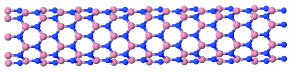
Figure 2: (color online) Boron nitride nanotube (8,0) with 256 atoms. The boron atoms are labeled as pink (light gray) balls while the nitrogen atoms are labeled as blue (dark gray) balls. The bond length between a pair of adjacent boron and nitride atoms is 1.45 Angstrom.

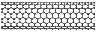
Figure 3: (color online) Carbon nanotube (8,8) with 512 atoms. The carbon atoms are labeled as gray balls. The bond length between a pair of adjacent carbon atoms is 1.42 Angstrom.

Our computational experiments were performed on the Hopper system at the National Energy Research Scientific Computing (NERSC) center. The performance results reported below were obtained from running the existing and modified codes on a single core of Hopper which is part of a node that consists of two twelve-core AMD ’MagnyCours’ 2.1-GHz processors. Each Hopper node has 32 gigabytes (GB) DDR3 1333-MHz memory. Each core processor has 64 kilobytes (KB) L1 cache and 512KB L2 cache. It also has access to a 6 megabytes (MB) of L3 cache shared among 6 cores.

Although the existing code has been parallelized using MPI and ScaLAPACK, the parallelization of selected inversion is still work in progress. Hence, the performance study reported here is limited to single processor runs. However, we expect that the new approach of using the PEXSI technique to compute the charge density, total energy, Helmholtz free energy and force will have a more favorable parallel scalability compared to diagonalizing the Kohn-Sham Hamiltonian by ScaLAPACK because it can take advantage of an additional level of parallelism introduced by the pole expansion. Due to the availability of such parallelism, the cost of the computational time of PEXSI is reported as the wall clock time for evaluating the selected elements of one single pole.

In addition to comparing the performance of the existing and new approaches in terms of wall clock time, we will also report the accuracy of our calculation and memory usage.

III.1 Atomic Orbitals and the Sparsity of $H$ and $S$

The electronic structure calculation code we used for the performance study is based on a local atomic orbital expansion scheme Chen et al. (2010, 2011). We will refer to this scheme as the CGH scheme below. In the CGH scheme, an atomic orbital $\varphi_{\mu}({\bf r})$ is expressed as the product of a radial wave function $f_{\mu,l}(r)$ and a spherical harmonic $Y_{lm}(\hat{r})$, where $\mu=\{\alpha,i,\zeta,l,m\}$, and $\alpha,i,\zeta,l,m$ represent the atom type, the index of an atom, the multiplicity of the radial functions, the angular momentum and the magnetic quantum number respectively. The radial function $f_{\mu,l}(r)$ is constructed as a linear combination of spherical Bessel functions within a cutoff radius $r_{c}$, i.e.,

$$f_{\mu,l}(r)=\left\{\begin{array}[]{ll}\sum_{q}c_{\mu q}j_{l}(qr),&r<r_{c}\\ 0&r\geq r_{c}\,.\\ \end{array}\right.$$ (34)

where $j_{l}(qr)$ is a spherical Bessel function with $q$ chosen to satisfy $j_{l}(qr_{c})$=0, and the coefficients $c_{\mu q}j_{l}(qr)$ are chosen to minimize a “spillage factor” Sánchez-Portal et al. (1995, 1996) associated with a reference system that consists of a set of (4 or 5) dimers. We refer readers to Ref. Chen et al., 2010, 2011 for the details on the construction of the CGH local atomic orbitals.

The cutoff radius $r_{c}$ determines the sparsity of the Kohn-Sham Hamiltonian $H$ and the overlap matrix $S$. The smaller the radius, the sparser $H$ and $S$ are. The cutoff radius for the atomic orbitals is set to $8.0$ Bohr for B and N atoms in BNNT, and $6.0$ Bohr for C atoms in CNT, respectively. The reasons why we choose a larger cutoff radius for B, N atoms is that the spillage factor for the B and N atoms is larger than that for the C atoms if $6.0$ Bohr cutoff is used for all atoms, which affects the accuracy of atomic orbitals. In general, the cutoff radius of most atomic orbitals can be chosen below $10$ Bohr.

Another parameter that affects the dimension of $H$ and $S$ is the multiplicity $\zeta$ of the radial function $f_{\mu,l}(r)$. The multiplicity determines the number of basis functions per atom. A higher multiplicity results in larger number of basis functions per atom, which in turn results in more rows and columns in $H$ and $S$. In our experiments, we used both single-$\zeta$ (SZ) orbitals and double-$\zeta$ plus polar orbitals (DZP). The number of local atomic orbitals is 4 for SZ and 13 for DZP.

We measure the sparsity by the percentage of the nonzero elements in the matrix $H$ denoted by

$$H_{\mathrm{nnz}}\%=\frac{\mathrm{nnz}(H)}{N^{2}(H)}\times 100.$$ (35)

Here $\mathrm{nnz}(H)$ is the number of nonzero elements of $H$ and $N(H)$ is the dimension of $H$ respectively. Since the computational cost of the selected inversion method is determined by the sparsity of $L+L^{T}$ for the Cholesky factor $L$ of $H-zS$, we will also report the percentage of the nonzero elements in the matrix $L+L^{T}$ (denoted by $L_{\mathrm{nnz}}\%$) below. To reduce the amount of non-zero fill-in of $L$, we use the nested dissection (ND) technique George (1973) to reorder the sparse matrix $H-zS$ before it is factored. Fig. 4 (a) depicts the sparsity pattern of the $H$ matrix associated with a 5120-atom BNNT (8,0) obtained from SZ atomic orbitals after it is reordered by ND. The sparsity pattern of $L+L^{T}$ for the corresponding Cholesky factor $L$ of the same problem is shown in Fig. 4 (b).

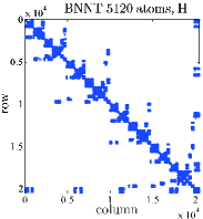
(a)

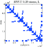
(b)

Figure 4: (color online) The sparsity pattern of $H$ (a) and $L+L^{T}$ (b) for an 5120-atom BNNT (8,0) with SZ orbitals. Nested dissection reordering is used.

Table 1 shows the sparsity of Hamiltonian matrices associated with BNNT (8,0) and CNT (8,8) systems that consist of $64$ to $10240$ atoms. The Hamiltonians for these systems are constructed from SZ atomic orbitals. We report both the $H_{\mathrm{nnz}}\%$ and $L_{\mathrm{nnz}}\%$ values. We can clearly see from this table that $H$, and consequently $L$, are quite dense when the number of atoms in the nanotubes is relatively small (less than 512). This is due to fact that a large percentage of atoms in these small systems are within the $r_{c}$ distance from each other. When the system size becomes larger (with more than $512$ atoms), both $H_{\mathrm{nnz}}\%$ and $L_{\mathrm{nnz}}\%$ are inversely proportional to the system size. This is because for quasi-1D systems, the numerator in Eq. (35) scales linearly with respect to $N(H)$ for large $N(H)$. Hence, the resulting matrices become increasingly sparse, thereby making the selected inversion method more favorable.

# Atoms		64	128	256	512	1024	1920	5120	10240
BNNT (8,0)	$H_{\mathrm{nnz}}\%$	100.00	85.54	42.77	21.43	11.69	5.70	2.13	1.06
	$L_{\mathrm{nnz}}\%$	100.00	99.48	77.94	46.13	25.07	13.70	5.26	2.64
CNT (8,8)	$H_{\mathrm{nnz}}\%$	40.63	38.67	19.53	9.77	4.88	2.60	0.97	0.49
	$L_{\mathrm{nnz}}\%$	69.92	68.45	68.70	54.38	31.75	17.54	7.42	3.79

Table 1: The percentage of nonzero elements $H_{\mathrm{nnz}}\%$ and $L_{\mathrm{nnz}}\%$ for BNNT (8,0) and CNT (8,8) of various sizes.

III.2 Performance comparison between diagonalization and selected inversion

We now compare the efficiency of selected inversion with that of diagonalization for computing the charge density in a single SCF iteration. In the existing code, the diagonalization of the matrix pencil $(H,S)$ is performed by using the LAPACK subroutine dsygv when the code is run on a single processor. The selected inversion is performed by the SelInv software Lin et al. (2011a).

We use BNNT(8,0) and CNT(8,8) nanotubes of different lengths to study the scalability of the computation with respect to the number of atoms in the nanotube. The number of atoms in these tubes ranges from $64$ to $10240$.

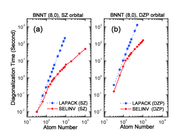
Figure 5: (color online) Comparisons of the wall clock time used by selected inversion (at one pole) required for PEXSI and by the LAPACK dsygv used to diagonalize a Kohn-Sham Hamiltonian associated with BNNT (8,0). The Hamiltonians are constructed from SZ orbitals (4 basis per atom) in (a) and DZP orbitals (13 basis per atom) in (b).

Fig. 5 shows how the wall clock time used by SelInv compares with that used by dsygv for BNNT(8,0) of different sizes. When SZ atomic orbitals are used, SelInv takes almost the same amount of time as that used by dsygv for a BNNT with $64$ atoms. When the number of atoms is larger than 64, SelInv is more efficient than dsygv. The cubic scaling of dsygv with respect to the number of atoms can be clearly seen from the slope of the blue loglog curve, which is approximately 3. The linear scaling of SelInv, which is indicated by the slope of the red curve, is evident when the number of atoms exceeds 200. For systems with less than 200 atoms, the wall clock time consumed by SelInv scales cubically with respect to the number of atoms also. This is due to the fact that the $H$ and $S$ matrices associated with these small systems are nearly dense. Similar observations can be made when the DZP atomic orbitals are used. In this case, SelInv is already more efficient than dsygv when the number of atoms is only 64. The linear scaling of SelInv can be observed when the number of atoms exceeds $128$.

Fig. 6 shows the timing comparison between SelInv and dsygv for CNT (8,8) of different sizes. Because the cutoff radius for the carbon atom is chosen to be 6.0, which is smaller than that associated with the boron and nitrogen atoms, the $H$ and $S$ matrices associated with CNT (8,0) are sparser even when the number of atoms in the tube is relatively small. This explains why SelInv is already more efficient than dsygv for a CNT with $64$ atoms regardless whether SZ or DZP atomic orbitals are used. However, the linear scaling of SelInv timing with respect to the number of atoms does not show up until the number of atoms reaches 500. The increase in the crossover point is due to the fact that the sparsity of $H$ is asymptotically determined by the number of atoms per unit length of the nanotube. Because the CNT (8,0) we use in our experiment has a large diameter, there are more atoms along the radial direction per unit length in CNT than that in BNNT. Consequently, it takes almost twice as many as atoms for CNT to reach the same length along the longitudinal direction when compared to BNNT, as we can see from Fig. 2 and Fig. 3.

We should note here that it is possible to combine the PEXSI technique with a SZ atomic orbital based Kohn-Sham DFT solver to perform electron structure calculation on quasi-1D systems with more than 10,000 atoms. On the Hopper machine, the wall clock time used to perform a single selected inversion of the $H-zS$ matrix associated with a 5,120-atom BNNT(8,0) is 26.72 seconds. When the number of atoms increases to 10240, the wall clock time increases to 50.07 seconds. Similar performance is observed for CNT(8,8). It takes 47.59 seconds to perform a selected inversion for a 5120-atom CNT(8,8) tube, and 97.16 seconds for a 10240-atom tube.

III.3 Memory usage

We should also remark that the memory requirement for SelInv increases linearly with respect to the number of atoms when the nanotube reaches a certain size. For a nanotube that consists of $10240$ atoms, the amount of memory required to store $L$ and the selected elements of $[H-(z_{l}+\mu)S]^{-1}$ is $0.66$ GB and $0.93$ GB respectively. The relatively low memory requirement of SelInv for quasi-1D system suggests that the method may even be applicable to quasi-1D systems that contain more than $100,000$ atoms on a single processor.

III.4 Accuracy

When selected inversion can be computed to high accuracy, which is often the case in practice, the only source of error introduced by the PEXSI technique comes from the limited number of terms in the pole expansion (15). The number of poles needed in (15) to achieve a desired level of accuracy in total energy (or free energy) and force is largely determined by the inverse temperature $\beta=1/(k_{B}T)$ used in (4) and the spectrum width $\Delta E$. Here we show that at room temperature $T=300K$, the number of poles required to provide an accurate pole expansion approximation is modest even for a metallic system such as CNT(8,8). Table 2 shows that when diagonalization is replaced by PEXSI for a single $\Gamma$-point calculation, the errors in total energy and force decrease as the number of poles in (15) increases. The force difference is measured between the force calculated by the PEXSI scheme using Eq. (27), and that calculated by the LAPACK diagonalization subroutine dsygv using standard methods Soler et al. (2002) previously implemented in the CGH atomic orbital scheme Chen et al. (2010, 2011). When the number of poles reaches 80, the difference between the final total energies produced by the existing code and the modified code (which replaces diagonalization with PEXSI) is $3.6\times 10^{-7}$ eV. The difference in the mean absolute error (MAE) is $2\times 10^{-6}$ eV/Angstrom, which is quite small for all practical purposes.

# Poles	$E_{\textrm{PEXSI}}-E_{\textrm{ref}}$ (eV)	MAE Force (eV/Angstrom)
20	5.868351108	0.400431
40	0.007370583	0.001142
60	0.000110382	0.000026
80	0.000000360	0.000002

Table 2: The difference between the total energy and atomic force produced by the existing electronic structure code and modified version in which diagonalization is replaced by PEXSI. The difference in atomic force is measured in terms of the mean absolute error (MAE).

The numbers of chemical potential iterations, as well as the error of the number of electrons at different SCF steps for a metallic CNT(8,8) system with $1024$ atoms using SZ basis set is reported in Fig. 7. The chemical potential is relaxed until the error associated with the total electron number ($4096$ electrons in this system) is within a given tolerance $\tau$. The average number of chemical potential iterations is $2.01$ for the low accuracy case ($\tau=10^{-1}$), and $5.21$ for the high accuracy case ($\tau=10^{-8}$), respectively. Notice that in both cases, the number of chemical potential iterations is $1\sim 2$ when the SCF gets close to convergence. Similar behavior is also observed in the geometry optimization example in section III.6 for which the change of chemical potential in consecutive steps is small. We further remark that the chemical potential does not need to be performed very accurately at the first few SCF steps. So the tolerance $\tau$ can be chosen dynamically with respect to the accuracy of the current SCF step, in order to further reduce the number of chemical potential iterations in the case of high accuracy calculation. We note that SelInv is a direct method for computing selected elements of the Green’s function accurately. When low accuracy is allowed, it is possible to reduce the computational cost of this method further by discarding elements in the Cholesky factor with small magnitude. This approach will be pursued in our future work.

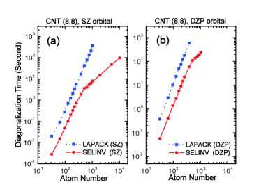
Figure 6: (color online) Comparisons of the wall clock time by selected inversion (at one pole) required for PEXSI and by the LAPACK dsygv used to diagonalize a Kohn-Sham Hamiltonian associated with CNT(8,8). The Hamiltonians are constructed from SZ orbitals (4 basis per atom) in (a) and DZP orbitals (13 basis per atom) in (b).

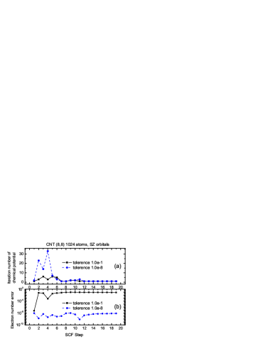
Figure 7: (color online) The numbers of chemical potential iteration steps (a), and the error associated with the number of electrons (b) at different SCF iterations for CNT(8,8) with $1024$ atoms using SZ basis set. The chemical potential is relaxed until the error of total number of electrons ($4096$ electrons in this system) is within $10^{-1}$ (blue dashed lines with dots) and within $10^{-8}$ (black solid lines with squares).

III.5 Overall Performance

One a sequential machine, the total wall clock time consumed by each PEXSI-based SCF iteration is $t_{selinv}\times P\times k_{\mu}$, where $t_{selinv}$ is the time required to perform one selected inversion, $P$ is the number of poles used in the pole expansion (13) and $k_{\mu}$ is the average number of chemical potential iterations. In practice, $P=80$ is often more than sufficient to yield an accurate approximation in (13) as we can see from Table 2. The average $k_{\mu}$ can be $1\sim 2$ especially in geometry optimization and molecular dynamics. If we take $P=80$ and $k_{\mu}=2$, the total wall clock time of a PEXSI-based SCF iteration is compared with an LAPACK diagonalization based SCF iteration for BNNT and CNT of various sizes in Fig. 8 and 9, respectively. Since the LAPACK diagonalization routine cannot perform as large of a calculation as PEXSI due to memory constraint, we extrapolate the wall clock time of the LAPACK diagonalization routine in Figures 8 and  9, and we find that the number of atoms beyond which the sequential PEXSI method outperform the diagonalization method is $1650$ atoms for BNNT(8,0) discretized by SZ orbital, and $1800$ atoms for BNNT(8,0) discretized by DZP orbital. Similarly, the crossover for the sequential PEXSI method to outperform the diagonalization method is $1750$ atoms for CNT(8,8) discretized by SZ orbitals, and $1700$ atoms for CNT(8,8) discretized by DZP orbitals.

However, when a large number of processors are available, the advantage of PEXSI becomes apparent. Because each term in (13) can be evaluated independently, we achieve an automatic $P$-fold speedup whereas the speedup that can be achieved by a parallel diagonalization procedure implemented in, for example, the ScaLAPACK software package, is often limited. Furthermore, each selected inversion can be parallelized, and our current work, which we will publish in a separate publication, indicates that excellent speedup can be achieved for this calculation on hundreds of processors. As a result, the PEXSI-based SCF iteration can easily scale to tens of thousands of processors, whereas it is difficult to make ScaLAPACK diagonalization procedures work efficiently on that many processors.

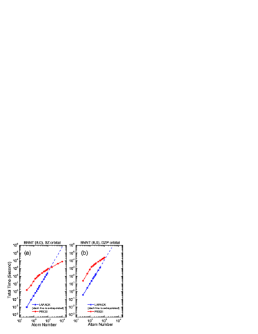
Figure 8: (color online) Comparisons of the total wall clock time used to perform a PEXSI-based SCF iteration (using 80 poles and $2$ iterations of chemical potential) and to perform an LAPACK dsygv diagonalization based SCF iteration for BNNT (8,0) configured with different numbers of atoms. The Hamiltonians are constructed from SZ orbitals (4 basis per atom) in (a) and DZP orbitals (13 basis per atom) in (b).

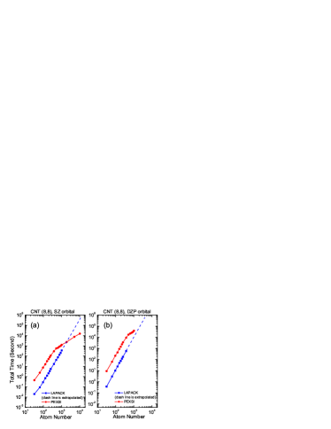
Figure 9: (color online) Comparisons of the total wall clock time used to perform a PEXSI-based SCF iteration (using 80 poles and $2$ iterations of chemical potential) and an LAPACK dsygv diagonalization based SCF iteration for CNT(8,8). The Hamiltonians are constructed from SZ orbitals (4 basis per atom) in (a) and DZP orbitals (13 basis per atom) in (b).

III.6 Geometry Optimization

The PEXSI scheme with atomic orbitals can also be used for accurate geometry relaxation of large-scale atomic systems. We use a truncated boron-nitride nanotube (8,0) with 1024 atoms, shown in Fig. 10, as an example to illustrate the efficiency of PEXSI in this type of calculation. The nanotube contains 504 boron atoms (B) and 504 nitride atoms (N). Each end of the nanotube is passivated by $8$ hydrogen atoms (H). We used DZP orbitals for all three atomic elements. The cutoff radius for B and N is set to 8.0 Bohr. The cutoff radius for H is set to 6.0 Bohr. We used 96 poles in the pole expansion for both energy and force calculations.

Convergence is reached after 105 steps of ionic relaxation steps are taken in the BFGS method. The maximum atomic force associated with the converged structure is less than 0.04 eV/Angstrom. To demonstrate the accuracy of the PEXSI method, we compare the differences of the atomic positions and forces obtained from separate geometry optimization simulations using the PEXSI method and the diagonalization method, starting from the same initial condition. Fig. 11 shows that at the $10$-th geometry optimization step, the maximum difference of the atomic positions among all $1024$ atoms is less than $5\times 10^{-7}$ Angstrom (Fig. 11 (a)), and the maximum difference of the forces is less than $2\times 10^{-5}$ eV/Angstrom (Fig. 11 (b)). Fig. 11 (c) shows that at the $10$-th geometry optimization step the absolute value of the force is still as large as $0.1\sim 1$ eV/Angstrom, and the relative error of the forces obtained from the PEXSI method is around $0.01\%$. This result shows that the PEXSI scheme is accurate for evaluating the forces for this system.

Figure 10: (color online) A truncated boron-nitride nanotube (8,0) with 1024 atoms, among which 504 boron atoms are labeled as pink (light gray) balls, 504 nitride atoms are labeled as blue (dark gray) balls, and 16 hydrogen atoms are labeled as small white balls. The hydrogen atoms are used to passivate both ends of the nanotube.

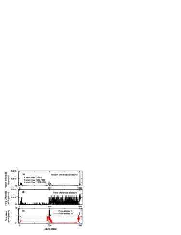
Figure 11: (color online) The differences of the atomic positions (a) and forces (b) obtained from separate simulations using the PEXSI method and the diagonalization method, starting from the same initial condition. The result is obtained at the $10$-th geometry optimization step for the boron-nitride nanotube (8,0) system with 1024 atoms. The absolute values of the forces at the $1$-st and the $10$-th geometry optimization steps are also presented (c). The tolerance for the error of the total number of electrons is chosen to be $10^{-8}$.

The convergence history of energy per atom and the convergence history of the maximum force with respect to the iteration number in the geometry optimization procedure are plotted in Fig. 12 (a) and (b), respectively. In Fig. 12 (a), the energy per atom at the last iteration step is set to zero. The energy per atom converges rapidly from 0.05 eV to 0.005 eV during the first 16 steps. Correspondingly, in Fig. 12 (b), the maximum force converges rapidly during the first few steps. This is mainly because the initial positions of the hydrogen and boron atoms near the end of the nanotube are not far from the equilibrium value. After the hydrogen and boron atoms at the boundary are relaxed to more reasonable positions, the maximum force begin to decrease slowly but with some oscillations. In order to illustrate more clearly the origin of the oscillation, we show the forces of boron atoms in Fig. 13. Fig. 13(a) and Fig. 13(b) show the forces of the boron atoms near the center of the nanotube and near the boundary of the nanotube, respectively. We find that the forces acting on the boron atoms near the center of the nanotube are much smaller than those near the boundary. This is mainly due to the fact that the atomic configuration near the center of the nanotube is close to the bulk configuration. The magnitude of the force acting on the atoms near the boundary is much larger, and is more difficult to convergence in the numerical optimization.

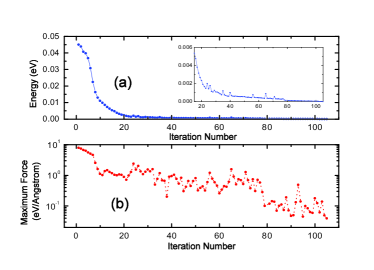
Figure 12: (color online) The energy per atom (a) and the maximum force (b) for each geometry optimization iteration step. The criterion for the convergence of the force is set to 0.04 eV/Angstrom. The energy per atom at the last iteration step is set to zero.

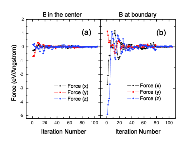
Figure 13: (color online) The force (x,y,z directions) acting on the boron atoms near the center of the nanotube (a) and near the boundary of the nanotube (b).

IV Conclusion

In this paper, we generalized the recently developed pole expansion and selected inversion technique (PEXSI) for solving finite dimensional Kohn-Sham equations obtained from an atomic orbital expansion. We gave expressions for evaluating the electron density, the total energy, the Helmholtz free energy and the atomic forces (including both the Hellman-Feynman force and the Pulay force) without using eigenvalues and eigenvectors of a Kohn-Sham Hamiltonian. These expressions are derived from an FOE approximation to the Fermi-Dirac function using an efficient and accurate pole expansion technique. The favorable $\log(\beta\Delta E)$ scaling of the pole expansion allows us to treat both insulating and metallic systems efficiently at room temperature or even lower temperature. The pole expansion only uses selected elements of the density matrix, energy density matrix and free energy density matrix. These selected elements can be obtained from computing the selected elements of the inverse of a shifted Kohn-Sham Hamiltonian through the selected inversion technique. The complexity of the selected inversion is $\mathcal{O}(N_{e})$ for quasi-1D systems such as nanorods, nanotubes and nanowires, $\mathcal{O}(N_{e}^{3/2})$ for quasi-2D systems such as graphene and surfaces, and $\mathcal{O}(N_{e}^{2})$ for 3D bulk systems. It compares favorably to the complexity of diagonalization, which is $\mathcal{O}(N_{e}^{3})$. We reported the performance achieved by comparing the efficiency of PEXSI with that of diagonalization on two types of nanotubes. The linear scaling behavior of PEXSI with respect to the number of atoms is clear when the number of atoms in these quasi-1D systems is larger than a few hundreds. For quasi-2D and quasi-3D systems, we expect the crossover point over which PEXSI exhibits $\mathcal{O}(N_{e}^{3/2})$ and $\mathcal{O}(N_{e}^{2})$ scaling to be much larger. However, based on the experiments presented here, PEXSI may still be more efficient than diagonalization (before the crossover point is reached) as long as the Cholesky factors of the shifted Kohn-Sham Hamiltonian are not completely dense.

The computational experiments we presented above were performed with a sequential implementation of the selected inversion algorithm. For quasi-1D systems such as nanotubes, the use PEXSI allows us to tackle problems that contain as many as 10,000 atoms. This cannot be done by using a diagonalization based approach. We further demonstrate the applicability of the PEXSI scheme by performing the geometry optimization of a truncated boron nitride nanotube with 1024 atoms. For quasi-2D and 3D systems, a parallel implementation of the PEXSI, which we are currently working on, is required to solve problems with that many atoms. We will report the performance for these large-scale calculations in a future publication.

Acknowledgment: This work was supported by the Laboratory Directed Research and Development Program of Lawrence Berkeley National Laboratory under the U.S. Department of Energy contract number DE-AC02-05CH11231 (L. L. and C. Y.), and by the Chinese National Natural Science Funds for Distinguished Young Scholars (L. H.).

Appendix

Derivation of Eq. (15):

$\Xi$ is a diagonal matrix, and the pole expansion (13) can be applied to each component of $\Xi$ as

$$f_{\beta}(\Xi-\mu)\approx\mathfrak{Im}\sum_{l=1}^{P}\frac{\omega^{\rho}_{l}}{\Xi-(z_{l}+\mu)I},$$ (36)

where $I$ is an $N\times N$ identity matrix. Using Eq. (12), the approximation of the single particle density matrix using $P$ terms of the pole expansion (still denoted by $\hat{\gamma}$ to simplify the notation) can be written as

$$\begin{split}\hat{\gamma}(x,x^{\prime})&=\Phi(x)C\mathfrak{Im}\sum_{l=1}^{P}\frac{\omega^{\rho}_{l}}{\Xi-z_{l}I}C^{T}\Phi^{T}(x^{\prime})\\ &=\Phi(x)\mathfrak{Im}\sum_{l=1}^{P}\frac{\omega^{\rho}_{l}}{C^{-T}\Xi C^{-1}-z_{l}C^{-T}C^{-1}}\Phi^{T}(x^{\prime}).\end{split}$$ (37)

Since the generalized eigenvalue problem (10) implies the identity

$$C^{T}HC=\Xi,\quad C^{T}SC=I,$$ (38)

the single particle density matrix takes the form

$$\hat{\gamma}(x,x^{\prime})=\Phi(x)\mathfrak{Im}\sum_{l=1}^{P}\frac{\omega^{\rho}_{l}}{H-(z_{l}+\mu)S}\Phi^{T}(x^{\prime})$$ (39)

which is Eq. (15).

Derivation of Eq. (24):

The first term in the Helmholtz free energy functional is

$$\begin{split}\operatorname{Tr}[f_{\beta}^{\mathcal{F}}(\Xi-\mu)]&=\operatorname{Tr}[Cf_{\beta}^{\mathcal{F}}(\Xi-\mu)C^{T}C^{-T}C^{-1}]\\ &\equiv\operatorname{Tr}[\Gamma^{\mathcal{F}}S].\end{split}$$ (40)

The second equal sign in Eq. (40) defines the free energy density matrix $\Gamma^{\mathcal{F}}$, which can be evaluated using the pole expansion (23) as

$$\begin{split}\Gamma^{\mathcal{F}}&=C\mathfrak{Im}\sum_{l=1}^{P}\frac{\omega^{\mathcal{F}}_{l}}{\Xi-z_{l}I}C^{T}\\ &=\mathfrak{Im}\sum_{l=1}^{P}\frac{\omega^{\mathcal{F}}_{l}}{C^{-T}HC^{-1}-z_{l}C^{-T}C^{-1}}\\ &=\mathfrak{Im}\sum_{l=1}^{P}\frac{\omega^{\mathcal{F}}_{l}}{H-z_{l}S},\end{split}$$ (41)

which is Eq. (24).

Derivation of Eq. (27):

The atomic force is in general given by the derivative of the Helmholtz free energy $\mathcal{F}_{\mathrm{tot}}$ with respect to the atomic positions. Since the free energy is minimized with respect to $\{\psi_{i}\}$,$\{f_{i}\}$ at each atomic configuration $\{R_{I}\}$, all the terms in $\mathcal{F}_{\mathrm{tot}}$ that do not explicitly depend on $R_{I}$ will not contribute to the atomic force $F_{I}$. In particular, the double counting terms $-\frac{1}{2}\iint\frac{\hat{\rho}(x)\hat{\rho}(y)}{\left\lvert x-y\right\rvert}\,\mathrm{d}x\,\mathrm{d}y+E_{{\mathrm{xc}}}[\hat{\rho}]-\int V_{{\mathrm{xc}}}[\hat{\rho}](x)\hat{\rho}(x)\,\mathrm{d}x$ do not contribute to the atomic force. Therefore

$$F_{I}=-\frac{d}{dR_{I}}\mathcal{F}_{\mathrm{tot}}=-\frac{\partial}{\partial R_{I}}\mathcal{F}_{\mathrm{tot}}.$$ (42)

Using the representation of the Helmholtz free energy in Eq. (20), and the fact that

$$(f_{\beta}^{\mathcal{F}})^{\prime}(z)=f_{\beta}(z),\qquad N_{e}=\operatorname{Tr}\left[f_{\beta}(\Xi-\mu)\right],$$ (43)

it can be derived that

$$\begin{split}F_{I}&=-\frac{\partial}{\partial R_{I}}\mathcal{F}_{\mathrm{tot}}=-\frac{\partial}{\partial R_{I}}\left(\operatorname{Tr}[f_{\beta}^{\mathcal{F}}(\Xi-\mu)]+\mu N_{e}\right)\\ &=-\operatorname{Tr}\left[(f_{\beta}^{\mathcal{F}})^{\prime}(\Xi-\mu)\left(\frac{\partial\Xi}{\partial R_{I}}-\frac{\partial\mu}{\partial R_{I}}\right)\right]-N_{e}\frac{\partial\mu}{\partial R_{I}}\\ &=-\operatorname{Tr}\left[f_{\beta}(\Xi-\mu)\frac{\partial\Xi}{\partial R_{I}}\right]-\frac{\partial\mu}{\partial R_{I}}\left(N_{e}-\operatorname{Tr}\left[f_{\beta}(\Xi-\mu)\right]\right)\\ &=-\operatorname{Tr}\left[f_{\beta}(\Xi-\mu)C^{T}\frac{\partial H}{\partial R_{I}}C\right]-\operatorname{Tr}\left[f_{\beta}(\Xi-\mu)\frac{\partial C^{T}}{\partial R_{I}}HC\right]\\ &\quad-\operatorname{Tr}\left[f_{\beta}(\Xi-\mu)C^{T}H\frac{\partial C}{\partial R_{I}}\right]\\ &=-\operatorname{Tr}\left[\Gamma\frac{\partial H}{\partial R_{I}}\right]-\operatorname{Tr}\left[f_{\beta}(\Xi-\mu)\frac{\partial C^{T}}{\partial R_{I}}HC\right]\\ &\quad-\operatorname{Tr}\left[f_{\beta}(\Xi-\mu)C^{T}H\frac{\partial C}{\partial R_{I}}\right]\\ \end{split}$$ (44)

The second and the third terms in Eq. (44) come from the nonorthogonality of the basis functions and should be further simplified. We have

$$\begin{split}&\operatorname{Tr}\left[f_{\beta}(\Xi-\mu)\frac{\partial C^{T}}{\partial R_{I}}HC\right]+\operatorname{Tr}\left[f_{\beta}(\Xi-\mu)C^{T}H\frac{\partial C}{\partial R_{I}}\right]\\ =&\operatorname{Tr}\left[(C^{-T}C^{-1})[C(C^{T}HC)f_{\beta}(\Xi-\mu)C^{T}](C^{-T}C^{-1})C\frac{\partial C^{T}}{\partial R_{I}}\right]\\ &+\operatorname{Tr}\left[C^{-T}C^{-1}[Cf_{\beta}(\Xi-\mu)(C^{T}HC)C^{T}]C^{-T}C^{-1}\frac{\partial C}{\partial R_{I}}C^{T}\right]\\ \equiv&\operatorname{Tr}\left[(C\Xi f_{\beta}(\Xi-\mu)C^{T})\left(SC\frac{\partial C^{T}}{\partial R_{I}}S+S\frac{\partial C}{\partial R_{I}}C^{T}S\right)\right].\end{split}$$ (45)

Define the energy density matrix as in Eq. (28), and Eq. (45) can be simplified as

$$\begin{split}&\operatorname{Tr}\left[\Gamma^{E}S\left(C\frac{\partial C^{T}}{\partial R_{I}}+\frac{\partial C}{\partial R_{I}}C^{T}\right)S\right]\\ =&\operatorname{Tr}\left[\Gamma^{E}S\frac{\partial S^{-1}}{\partial R_{I}}S\right]=-\operatorname{Tr}\left[\Gamma^{E}\frac{\partial S}{\partial R_{I}}\right]\end{split}$$ (46)

Combining Eq. (46) and Eq. (44), we have

$$F_{I}=-\frac{\partial\mathcal{F}}{\partial R_{I}}=-\operatorname{Tr}\left[\Gamma\frac{\partial H}{\partial R_{I}}\right]+\operatorname{Tr}\left[\Gamma^{E}\frac{\partial S}{\partial R_{I}}\right].$$ (47)

which proves Eq. (27).

References

- Bowler et al. (2002) D. R. Bowler, T. Miyazaki, and M. J. Gillan, J. Phys.: Condens. Matter 14, 2781 (2002).
- Fattebert and Bernholc (2000) J. L. Fattebert and J. Bernholc, Phys. Rev. B 62, 1713 (2000).
- Hine et al. (2009) N. D. Hine, P. D. Haynes, A. A. Mostofi, C. K. Skylaris, and M. C. Payne, Comput. Phys. Commun. 180, 1041 (2009).
- Yang (1991) W. Yang, Phys. Rev. Lett. 66, 1438 (1991).
- Li et al. (1993) X.-P. Li, R. W. Nunes, and D. Vanderbilt, Phys. Rev. B 47, 10891 (1993).
- McWeeny (1960) R. McWeeny, Rev. Mod. Phys. 32, 335 (1960).
- Goedecker (1999) S. Goedecker, Rev. Mod. Phys. 71, 1085 (1999).
- Bowler and Miyazaki (2012) D. R. Bowler and T. Miyazaki, Rep. Prog. Phys. 75, 036503 (2012).
- Kohn (1996) W. Kohn, Phys. Rev. Lett. 76, 3168 (1996).
- Prodan and Kohn (2005) E. Prodan and W. Kohn, Proc. Natl. Acad. Sci. 102, 11635 (2005).
- Lin et al. (2009a) L. Lin, J. Lu, L. Ying, and W. E, Chinese Ann. Math. 30B, 729 (2009a).
- Baroni and Giannozzi (1992) S. Baroni and P. Giannozzi, Europhys. Lett. 17, 547 (1992).
- Goedecker (1993) S. Goedecker, Phys. Rev. B 48, 17573 (1993).
- Ozaki (2007) T. Ozaki, Phys. Rev. B 75, 035123 (2007).
- Ceriotti et al. (2008) M. Ceriotti, T. Kühne, and M. Parrinello, J. Chem. Phys. 129, 024707 (2008).
- Ozaki (2010) T. Ozaki, Phys. Rev. B 82, 075131 (2010).
- Lin et al. (2009b) L. Lin, J. Lu, L. Ying, R. Car, and W. E, Comm. Math. Sci. 7, 755 (2009b).
- Lin et al. (2011a) L. Lin, C. Yang, J. Meza, J. Lu, L. Ying, and W. E, ACM. Trans. Math. Software 37, 40 (2011a).
- Lin et al. (2011b) L. Lin, C. Yang, J. Lu, L. Ying, and W. E, SIAM J. Sci. Comput. 33, 1329 (2011b).
- Varga (2010) K. Varga, Phys. Rev. B 81, 045109 (2010).
- Frisch et al. (1984) M. Frisch, J. Pople, and J. Binkley, J. Chem. Phys. 80, 3265 (1984).
- VandeVondele et al. (2005) J. VandeVondele, M. Krack, F. Mohamed, M. Parrinello, T. Chassaing, and J. Hutter, Comput. Phys. Commun. 167, 103 (2005).
- Junquera et al. (2001) J. Junquera, O. Paz, D. Sanchez-Portal, and E. Artacho, Phys. Rev. B 64, 235111 (2001).
- Chen et al. (2010) M. Chen, G. C. Guo, and L. He, J. Phys.: Condens. Matter 22, 445501 (2010).
- Chen et al. (2011) M. Chen, G. C. Guo, and L. He, J. Phys.: Condens. Matter 23, 325501 (2011).
- Kenny et al. (2000) S. D. Kenny, A. P. Horsfield, and H. Fujitani, Phys. Rev. B 62, 4899 (2000).
- Ozaki (2003) T. Ozaki, Phys. Rev. B 67, 155108 (2003).
- Blum et al. (2009) V. Blum, R. Gehrke, F. Hanke, P. Havu, V. Havu, X. Ren, K. Reuter, and M. Scheffler, Comput. Phys. Commun. 180, 2175 (2009).
- Tsuchida and Tsukada (1998) E. Tsuchida and M. Tsukada, J. Phys. Soc. Jpn. 67, 3844 (1998).
- Lin et al. (2012) L. Lin, J. Lu, L. Ying, and W. E, J. Comput. Phys. 231, 2140 (2012).
- Lin et al. (2009c) L. Lin, J. Lu, R. Car, and W. E, Phys. Rev. B 79, 115133 (2009c).
- Lanczos (1950) C. Lanczos, J. Res. Nat. Bur. Stand. 45, 255 (1950).
- Chelikowsky et al. (1994) J. Chelikowsky, N. Troullier, and Y. Saad, Phys. Rev. Lett. 72, 1240 (1994).
- Tsuchida and Tsukada (1995) E. Tsuchida and M. Tsukada, Phys. Rev. B 52, 5573 (1995).
- Mermin (1965) N. Mermin, Phys. Rev. 137, A1441 (1965).
- Soler et al. (2002) J. M. Soler, E. Artacho, J. D. Gale, A. García, J. Junquera, P. Ordejón, and D. Sánchez-Portal, J. Phys.: Condens. Matter 14, 2745 (2002).
- Kresse and Furthmüller (1996) G. Kresse and J. Furthmüller, Phys. Rev. B 54, 11169 (1996).
- Weinert and Davenport (1992) M. Weinert and J. W. Davenport, Phys. Rev. B 45, 13709 (1992).
- Wentzcovitch et al. (1992) R. M. Wentzcovitch, J. L. Martins, and P. B. Allen, Phys. Rev. B 45, 11372 (1992).
- Alavi et al. (1994) A. Alavi, J. Kohanoff, M. Parrinello, and D. Frenkel, Phys. Rev. Lett. 73, 2599 (1994).
- Ceperley and Alder (1980) D. M. Ceperley and B. J. Alder, Phys. Rev. Lett. 45, 566 (1980).
- Becke (1988) A. D. Becke, Phys. Rev. A 38, 3098 (1988).
- Lee et al. (1988) C. Lee, W. Yang, and R. G. Parr, Phys. Rev. B 37, 785 (1988).
- Pulay (1969) P. Pulay, Mol. Phys. 17, 197 (1969).
- Sankey and Niklewski (1989) O. F. Sankey and D. J. Niklewski, Phys. Rev. B 40, 3979 (1989).
- Charlier et al. (2007) J.-C. Charlier, X. Blase, and S. Roche, Rev. Mod. Phys. 79, 677 (2007).
- Sánchez-Portal et al. (1995) D. Sánchez-Portal, E. Artacho, and J. M. Soler, Solid State Commun. 95, 685 (1995).
- Sánchez-Portal et al. (1996) D. Sánchez-Portal, E. Artacho, and J. M. Soler, J. Phys.: Condens. Matter 8, 3859 (1996).
- George (1973) A. George, SIAM J. Numer. Anal. 10, 345 (1973).