Exponential speed of mixing for skew-products with singularities

Abstract

Let $f:[0,1]\times[0,1]\backslash\{1/2\}\to[0,1]\times[0,1]$ be the $C^{\infty}$ endomorphism given by

$$f(x,y)=\left(2x-\lfloor 2x\rfloor,\,y+\frac{c}{|x-1/2|}-\left\lfloor y+\frac{c}{|x-1/2|}\right\rfloor\right),\;c\in\mbox{$I\!\!R$}^{+}$$

We prove that $f$ is topologically mixing and if $c>1/4$ then $f$ is mixing with respect to Lebesgue measure. Furthermore we prove that the speed of mixing is exponential.

2000 Mathematics Subject Classification: 37D30, 37C29, 37E30.
Keywords: skew-product with singularities, ergodicity, mixing, rate of mixing.

1 Introduction

A basic problem in dynamics is the understanding of the ergodic behavior of a given dynamical system. Frequently this is translated into the knowledge of mixing properties of the system. Once mixing is established it is natural to ask for the rate or speed of mixing of the system.

For hyperbolic systems and nonuniform hyperbolic ones , without or with singularities, this kind of study is well understood and the techniques to do so have been developed by several authors. We indicate the works by Sinai [Si], Pesin [Pe], Pesin and Barreira, [BP], Dolgopyat [Do], Ruelle [Ru], Bowen [Bo], L-S Young [Yo1][Yo2], Benedicks [BY], Baladi [Ba], Viana [Vi], Walters [Wa], and the references therein to the interested reader.

When the system $T$ under study has singularities, the phase space is not the whole manifold and in this case one asks zero-Lebesgue measure for the union $\cup_{n=0}^{\infty}T^{-n}S$ of the set of singularities $S$. This is the case of billiards, studied by Sinai, Chernov [Ch],[CY], Markarian [CM], Bunimovich [Bu] and others. In these cases we have the additional difficulty that the stable and unstable manifolds of points may be arbitrarily short since their length is conditioned by the distance of the points to $S$.

In general, the presence of singularities adds complexity into the problem and makes the analysis much more difficult. Nevertheless, in this paper, where we study a certain skew-product with singularities on the fiber, it is the presence of singularities, jointly with the expanding action in the base that enable us to obtain all the chaotic behavior of the system.

In this paper we are interested in the mixing properties of the skew-product given by the $C^{\infty}$-endomorphism $f:[0,1]\times\big{(}[0,1]\backslash\{1/2\}\big{)}\to[0,1]\times[0,1]$ defined by

$$f(x,y)=\left(2x-\lfloor 2x\rfloor,\,y+\frac{c}{|x-1/2|}-\left\lfloor y+\frac{c}{|x-1/2|}\right\rfloor\right),\;c\in\mbox{$I\!\!R$}^{+}.$$

Here, given a real number $x$, $\lfloor x\rfloor$ stands for the greatest integer less or equal to $x$.

Since the denominator $\frac{c}{|x-1/2|}$ vanishes at $x=1/2$, the line $\{(1/2,y)\,:\;y\in[0,1)\}$ is constituted by singularities of $f$. Besides that, for $c\neq 0$ we have that the vertical projection of $f(x,y)$ sharply varies when $x\approx 1/2$.

Identifying $[0,1]\times[0,1]$ with the two-dimensional torus ${\Bbbten T}^{2}$, the skew-product may be seen as defined in ${\Bbbten T}^{2}$ where the circle given by $x=1/2$ is a curve of singularities of $f$.

The successive iterates by $f$ of a rectangle $R$ are transformed into a denumerable set of strips accumulating onto the circle $x=1$ in the torus. This effect together with the fact that the pre-orbit by $x\mapsto 2x\mod(1)$ of the circle $x=1/2$ is dense in the torus are responsible of the rich chaotic dynamics observed in this system.

Since the length of vertical segments are preserved under $f$, the action of $f$ on the vertical borders of $R$ is just a translation depending continously on $x\in[0,1]\setminus\{1/2\}$. Hence, the stretching and accumulation of the iterates of $R$ onto the pre-orbit of the circle $x=1/2$ in the torus is due to the slipping effect of $f$ in the horizontal borders of $R$.

The skew-product $f$ can be also immersed in a one-parameter family of expanding skew-products with the same line of singularities:

$$f_{\lambda}(x,y)=(2x,\lambda y+\frac{c}{|x-1/2|}),\,\,\lambda\geq 1\,.$$

Thus, it is interesting to detected the ergodic properties in the limit dynamics given by $\lambda=1$. For instance, transitivity, mixing and rate of mixing.

In this paper we prove that the skew-product $f$ is topologically mixing, preserves the Lebesgue measure $m$ on the torus, is mixing with respect to $m$ and finally we prove that the rate of mixing is exponential.

1.1 Toy model of flows with a singularity: slipping effect.

Let $M$ be a $3$-dimensional manifold and assume that $\Phi:M\to M$ is a flow containing a transitive attractor $\Lambda\subset M$ with a hyperbolic singularity $p\in\Lambda$. The geometric Lorenz attractor and any Lorenz-like attractor satisfy these conditions, see [GW, Lo, AP].

We consider the case when the singularity has three real eigenvalues $\lambda_{i}$, $1\leq i\leq 3$, and satisfy $\lambda_{2}(\sigma)<\lambda_{3}(\sigma)<0<-\lambda_{3}(\sigma)<\lambda_{1}(\sigma)$. Via Hartmann-Großman theorem we assume that we have linearized coordinates in a neighborhood $U\supset[-1,1]^{3}$ of the singularity $p$ in such a way that $\lambda_{1}$ corresponds to $0x$-axis, $\lambda_{2}$ to $0y$-axis and $\lambda_{3}$ to $0z$-axis.

Let $S=\{(x,y,z)\in U\,:\,z=1\}$ be a transverse section to the flow so that every trajectory eventually crosses $S$ in the direction of the negative $z$-axis. Consider also $\Sigma=\{(x,y,z):|x|=1\}=\Sigma^{+}\cup\Sigma^{-}$ with $\Sigma^{\pm}=\{(x,y,z):x=\pm 1\}\,.$ To each $(x_{0},y_{0},1)\in S$ the time $\tau$ such that $X^{\tau}(x_{0},y_{0},1)\in\Sigma$ is given by $\tau(x_{0})=\frac{-1}{\lambda_{1}}\log|x_{0}|$, and it is such that $\tau(x_{0})\to\infty$ when $x_{0}\to 0$. This fact has the effect that different slices parallel to $0y$-axis of the section $S$ arrives to $\Sigma$ with a delay. Hence, we cannot see the return of each slice to $S$ at the same time, even when the expecting delay is bounded .

Assume now that we ”forget” the effect of the singularity and consider that the return time is the same for points in a same slice. Also ”forget” the strong stable direction. Note that the strong stable direction does not interfere in the dynamics of the geometric Lorenz attractor.

After these identifications, the dynamics in a neighborhood of $p$ occurs in the $(x,z)$ plane, and may be seen as a slipping in the vertical direction in order to annihilate the delay of time. Since the delay goes to infinity as $x\to 0$ the slipping also goes to infinity when $x\to 0$. Thus, the dynamics there is given by $(\phi(x),\psi(x,z))$ with $\psi(x,z)\to\infty$ when $x\to 0$. Moreover, since the ratio $\beta=-\frac{\lambda_{2}}{\lambda_{1}}$ is greater than one, the dynamics in the $x$ direction is expanding.

Thus, changing the name of the variable $z$ by $y$, the skew-product

$$f(x,y)=\left(2x\mod(1),y+\frac{c}{|x-1/2|}\mod(1)\right)$$

may be seen as a simplified case of the slipping effect in singular hyperbolic attractors, as is the case of a Lorenz-like attractor.

1.2 Statement of results.

To announce in a precise way our results let us introduce some definitions and related facts proved elsewhere.

Definition 1.1.

Let $(X,\mathcal{A},f,\mu)$ be a dynamical system defined on the space $X$, $\mathcal{A}$ a $\sigma$-algebra of $X$, and $\mu$ an $f$-invariant probability measure. The map $f$ is mixing if for all pair of sets $A,B\in\mathcal{A}$, we have

$$\lim_{n\to\infty}\mu(f^{-n}(A)\cap B)=\mu(A)\mu(B)\,.$$

A form of mixing that can be defined without appealing to measures is the following

Definition 1.2.

Let $f:X\to X$ be a continuous map defined in the topological space $X$. We say that the dynamical system defined by $f$ is topologically mixing if for every pair of non-empty open subsets $A,\,B$ of $X$ there is $N>0$ such that $\forall n\geq N:\,f^{n}(A)\cap B\neq\emptyset$.

There is even a commonly used weaker notion: we say that the system defined by $f$ is topologically transitive if for every pair of non-empty open subsets $A,\,B$ of $X$ there is $n\in\mbox{$Z\!\!\!Z$}$ such that $f^{n}(A)\cap B\neq\emptyset$.

It is well known that if a dynamical system is defined on topological space $X$, $\mathcal{A}$ is the Borel $\sigma$-algebra of $X$ and $\mu$ is a probability invariant measure such that $\mu(A)>0$ for every open set $A$ of $X$, then if the system is mixing it is topological mixing. This and other general results on Ergodic Theory may be found in [Wa], for instance.

The main results in this paper are:

Theorem A.

For all positive $c$ the skew-product $f:{\Bbbten T}^{2}\to{\Bbbten T}^{2}$ is topologically mixing.

Theorem B.

The skew-product $f$ preserves the Lebesgue measure $m$ in the torus and, for $c>1/4$, $f$ is mixing with respect to $m$.

Theorem C.

The rate of mixing is exponential, that is, there is $0<\lambda<1$ such that for all pair of sets $A$ and $B$ we have

$$|m(f^{-n}(A)\cap B)-m(A)m(B)|<\lambda^{n}m(A)m(B),\quad\mbox{ for all}\quad n\geq 0\,.$$

Next we list two interesting features of the skew-product $f$

• For all $p=(x,y)\in{\Bbbten T}^{2}$, there is no stable manifold $W^{s}(p,f)$. Indeed, given $(x,y)$ and $(x+\Delta x,y+\Delta y)$, assuming that $x<1/2$, $\Delta x\neq 0$, $x+\Delta x<1/2$ and computing

  $$\|f(x+\Delta x,y+\Delta y)-f(x,y)\|=\left\|2\Delta x,\Delta y+\frac{c}{1/2-x}\left[\frac{1}{1-\frac{\Delta x}{1/2-x}}-1\right]\mod 1\right\|\geq$$

  $$\geq 2|\Delta x|,\;\mbox{ and similar result holds for }\;x>1/2\,.$$

  Hence, if $\Delta x\neq 0$, ${\rm dist}(f^{n}(x+\Delta x,y+\Delta y),f^{n}(x,y))\geq 2^{n}\Delta x\mod 1$ which does not converges to 0. On the other hand, if $\Delta x=0$ then the distance between $f^{n}(x,y+\Delta y)$ and $f^{n}(x,y)$ is preserved. Thus, for no $(\Delta x,\Delta y)$ we have ${\rm dist}(f^{n}(x+\Delta x,y+\Delta y),f^{n}(x,y))\to 0$ when $n\to+\infty$.

• The unstable manifolds are not unique. Indeed, for any itinerary $\{(x_{n},y_{n})\}_{n\in\mbox{$I\!\!N$}}$ such that $f(x_{n},y_{n})=(x_{n-1},y_{n-1})$ it is defined an unstable manifold $W^{u}((x_{0},y_{0}),f)$ (recall that $f$ is an endomorphism) and so the unstable manifold of a point is not unique. Moreover, $f$ is not an expanding map since for any $p=(x,y)$ we have $Df_{p}(0,1)=(0,1)$. Finally, it has no dominated splitting (see Section 2 for the proof of these facts).

Thus, the standard techniques in dynamics using existence of stable and unstable manifolds, for instance, are useless here.

2 Preliminaries

In this section we establish some preliminaries properties of $f$ that will be used in the proofs. We identify the set $Q=[0,1]\times[0,1]$ with the 2-torus ${\Bbbten T}^{2}$.

If $0\leq x<1/2$ then we have that $f(x,y)=(2x,y+\frac{c}{1/2-x}-\lfloor y+\frac{c}{1/2-x}\rfloor)$ while if $1/2<x<1$ then $f(x,y)=(2x-1,y+\frac{c}{x-1/2}-\lfloor y+\frac{c}{x-1/2}\rfloor)$.

The matrix $\left[Df_{(x,y)}\right]$ is in the case $0\leq x<1/2$ given by $\left(\begin{array}[]{cc}2&0\\ \frac{c}{(1/2-x)^{2}}&1\\ \end{array}\right)$ and in the case $1/2<x\leq 1$ by $\left(\begin{array}[]{cc}2&0\\ \frac{-c}{(1/2-x)^{2}}&1\\ \end{array}\right)$. Therefore it depends only on $x$. Any vector different of a vertical one is expanded by the action of $Df$ which presents two eigenvalues: $1$ with eigenvector $(0,1)$, and $2$ with eigenvector $(1,\frac{c}{(x-1/2)^{2}})$ if $0\leq x<1/2$ and $(-1,\frac{c}{(x-1/2)^{2}})$ if $1/2<x<1$. Hence we have no stable manifold at any point of ${\Bbbten T}^{2}$ (see $(\star)$  ) and points at the left of the line $x=1/2$ have eigenvectors corresponding to the eigenvalue 2 forming an acute angle with the $Ox$ axis such that when $x\to 1/2$ the angle between the eigenvector associated to 2 tends to be vertical. A similar picture is valid at points at the right of $x=1/2$ taking into account that in that case the eigenvector associated to 2 forms an obtuse angle with the $Ox$ axis. From these facts one may see that no non-trivial splitting is preserved. Indeed, given a periodic orbit, no direction different of the vertical one is preserved.

Given a real number $a\in(0,1)$, we write

$$a=\sum_{1}^{\infty}\frac{a_{i}}{2^{i}},\;\;\;a\sim 0.a_{1}\cdots a_{n}\cdots\quad a_{j}\in(0,1)$$

for its binary decomposition.

Writing $x\in[0,1)$ in base $2$ the dynamics in the $x$- coordinate is as the shift

$$\sigma:\{0,1\}^{\mbox{$I\!\!N$}}\to\{0,1\}^{\mbox{$I\!\!N$}},\quad\sigma(b_{1}b_{2}b_{3}\cdots)=b_{2}b_{3}\cdots$$

Each point $x\sim(b_{1}b_{2}\cdots)$ has two pre-images by this map

$$\sigma^{-1}(b_{1}b_{2}\cdots)=\left\{\begin{array}[]{l}x_{0}\sim(0\,b_{1}b_{2}\cdots)\sim x/2\\ x_{1}\sim(1\,b_{1}b_{2}\cdots)\sim(1+x)/2\end{array}\right.$$ (1)

Since $f(x,y)=(2x,y+c/|x-1/2|)\mod(1)$ equation (1) implies that any $Z=(x,y)\in{\Bbbten T}^{2}$, with $x=0.b_{1}b_{2}\cdots$ has two pre-images $Z_{0},\,Z_{1}$ by $f$ given by:

1. $Z_{0}=\left(\frac{x}{2},y-\frac{2c}{1-x}-\lfloor y-\frac{2c}{1-x}\rfloor\right)=(x_{0},y_{0}),$

2. $Z_{1}=\left(\frac{1+x}{2},y-\frac{2c}{x}-\lfloor y-\frac{2c}{x}\rfloor\right)=(x_{1},y_{1}).$

Inductively, given a sequence ${{b}}=(b_{1}b_{2}\cdots b_{n})$ of length $|b|=n$, with $b_{j}\in\{0,1\},\,\,\forall j\leq n$, and assuming that $Z_{b_{2}b_{3}\cdots b_{n}}$ (one of the $(n-1)$-th preimages of $Z$)is already defined we have that one of the $n$-th preimages of $Z$ is $Z_{{{b}}}=(x_{{{b}}},y_{{{b}}})$ with

$$(a)\hskip 76.82234ptx_{{{b}}}=\frac{b_{1}+x_{b_{2}b_{3}\cdots b_{n}}}{2}\qquad\hskip 85.35826pt$$ (2)

and

$$(b)\quad y_{{{b}}}=\left(y_{b_{2}\cdots b_{n}}-\frac{2c}{(1-b_{1})+(2b_{1}-1)x_{b_{2}\cdots b_{n}}}\right)\mod(1)$$

We remark that if $Z=(x,y),\;\;W=(x^{\prime},y^{\prime})$ and $b=(b_{1}b_{2}\cdots b_{n})$ then $|x_{b}-x^{\prime}_{b}|=|x-x^{\prime}|/2^{n}$. We also remark that for any $x\in[0,1)$ the set of preimages $\mathcal{S}_{n}$ of $x$ for all the different $b$’s of length $n$ is almost uniformly distributed in $[0,1)$, i.e., for any interval $I\subset[0,1)$:

$$\lim_{n\to\infty}\frac{\#(\mathcal{S}_{n}\cap I)}{\#\mathcal{S}_{n}}=\ell(I).$$ (3)

Here $\#X$ means the cardinality of $X$ ($\#S_{n}=2^{n}$), and $\ell(I)$ is the length of $I$.

We extend this notation to the $n$-th preimage of an horizontal segment $I=[Z,Y]$: $Z_{b}(I)$ is the $n$-th pre-image of $I$ that has $Z_{b}$ as one of its boundaries. In the same way, if $R$ is a rectangle whose lower bound is $I$, then $Z_{b}(R)$ is the $n$-th pre-image of $R$ with $Z_{b}(I)$ as one of its “sides”.

Lemma 2.1.

The vertical projection $\Pi_{y}(f(\gamma))$ of the image of a monotone arc $\gamma(t)=(x(t),y(t))$ (i.e., an arc such that $x(t)$ and $y(t)$ are monotone functions) whose horizontal projection $\Pi_{x}(\gamma)$ has length greater or equal to $2/c$ covers all $[0,1)$.

Proof.

Given a monotone arc $\gamma:[0,1]\to{\Bbbten T}^{2}$, $\gamma(t)=(x(t),y(t))$, the vertical projection of the function $f(x(t),y(t))=(2x(t)\mod(1),y(t)+\frac{c}{|x(t)-1/2|}\mod(1))$ varies from $y(0)+\frac{c}{|x(0)-1/2|}\mod(1)$ to $y(1)+\frac{c}{|x(1)-1/2|}\mod(1)\,,$ covering $|y(1)-y(0)+\frac{c}{|x(1)-1/2|}-\frac{c}{|x(0)-1/2|}|\mod(1)$.

In order to simplify computations we suppose that $\gamma$ is in $\mbox{$I\!\!R$}^{2}$. Then if its horizontal projection includes $k+1/2,k\in\mbox{$Z\!\!\!Z$}$ the vertical projection has infinite length. Assume now that $3/2>x(1)>x(0)+2/c>x(0)>1/2.$ Thus,

$$\left|\frac{c}{|x(1)-1/2|}-\frac{c}{|x(0)-1/2|}\right|=\left|\frac{c}{x(1)-1/2}-\frac{c}{x(0)-1/2}\right|>c\frac{x(1)-x(0)}{(x(1)-1/2)(x(0)-1/2)}>4\,.$$

Thus, since $-1\leq y(1)-y(0)\leq 1$ we have $|y(1)-y(0)+\frac{c}{|x(1)-1/2|}-\frac{c}{|x(0)-1/2|}|>2$. ∎

3 The skew-product is topologically mixing

Recall that a map $f:M\to M$ is topologically mixing if for all pair of open sets $A,B$ of $M$ there is $N$ such that for all $n\geq N$ it holds $f^{n}(A)\cap B\neq\emptyset$.

Theorem 3.1.

If $c\in\mbox{$I\!\!R$}^{+}$ then $f(x,y)$ is topologically mixing.

Proof.

It is enough to prove the statement for open rectangles $A$ and $B$ of sides parallel to the coordinate axes since they form a basis for the standard topology of the plane.

The idea of the proof is as follows: Let $(x_{A},y_{A})$ be the coordinates of the center of $A$ and $(x_{B},y_{B})$ the coordinates of the center of $B$. We pick a suitable pre-image of $(x_{B},y_{B})$, $Z_{{{r}}}=(x_{{{r}}},y_{{{r}}})$, as in (2) so that $Z_{r}$ is close to $(x_{A},y_{A})$ and such that for some $n$, with $0<n<|r|$, it holds that $f^{n}(Z_{r})$ is in a small enough neighborhood of $\{x=1/2\}$ to guarantee that the pre-image of $Z_{r_{n}}(S)$ (here $r_{n}$ represents the sub-string of length $n$ contained in $r$), where $S$ is the horizontal segment contained in $B$ and passing through $(x_{B},y_{B})$, is almost vertical and has length greater than 1. This implies that the pre-image $Z_{r}(S)$ cuts $A$ and thus we obtain that $f^{|r|}(Z_{r}(S))$ cuts $B$.

To begin with the proof let $2\delta_{A}$ be the length of $\Pi_{x}(A)$ and $2\delta_{B}$ the length of $\Pi_{x}(B)$. Let also, in base 2, $x_{A}=(0.a_{1}a_{2}a_{3}\ldots)_{2}$ and $x_{B}=(0.b_{1}b_{2}b_{3}\ldots)_{2}$ and find $N$ such that for $\delta=\min\{\delta_{A},\delta_{B}\}$ we have $1/2^{N}<\delta$ and so $2^{N}\,\delta>1$. Now we consider

$$r=0.a_{1}a_{2}\ldots a_{N}0\underset{N\text{ ones}}{\underbrace{11\ldots 1}}0b_{1}b_{2}b_{3}\ldots b_{N}\,.$$

Clearly $\Pi_{x}(Z_{r})$ is near $x_{A}$ and lies in $[x_{a}-\delta_{A},x_{A}+\delta_{A}]$ since $|x_{r}-x_{A}|<1/2^{N}$. Now we choose $y_{r}\in(0,1)$ such that $\Pi_{y}(Z_{r})$ belongs to $y=y_{A}$.

After $N$ iterates by $f$ we have that $f^{N}(Z_{r})$ is at a distance less that $1/2^{N}$ from $\{x=1/2\}$ (since $\Pi_{x}(f^{N}(Z_{r}))=0.011\ldots 10b_{1}b_{2}b_{3}\ldots\,$).

It holds that the vertical projection of $f^{N}(A)$ has length greater than 1 and $\Pi_{x}(f^{2N+2}(Z_{r}))\in\Pi_{x}(B)$ and $\ell(\Pi_{y}(f^{2N+2}(A)))>1$ too. Therefore $f^{2N+2}(A)\cap B\neq\emptyset$.

Since the length of the horizontal projection doubles under iterations by the action $x\mapsto 2x\mod 1$, there is $N_{1}>0$ such that for $n>N_{1}$ we have that $\Pi_{x}(f^{n}(A))$ covers all $[0,1]$. It follows that $f^{N_{1}+2N+2+k}(A)\cap B\neq\emptyset$ for all $k\geq 0$. Thus $f$ is topologically mixing, proving Theorem A ∎

4 Lebesgue measure preserved and mixing.

In this section we prove Theorem B. We start establishing some auxiliary lemmas. The first says that even for the worst case, if $c>1/4$ we have that the preimages by $f$ expand length in the vertical direction.

Lemma 4.1.

There is $N(c)=N>0$ such that for $n\geq N$, every horizontal arc $I,$ $l(I)=\Delta x$, every $b=b_{1}b_{2}\cdot b_{n}$ it results $l(Z_{b}(I))>4c\Delta x$ ($l$ is the euclidean length in the torus).

Proof.

Given a segment $[x,x+\Delta x]\subset[0,1/2)$, the length of its image by any of its branches: $Z_{0},\,Z_{1}$ is given by

$$\int_{x/2}^{x/2+\Delta x/2}\sqrt{1+\frac{c^{2}}{(1/2-s)^{4}}}\,ds\geq\left.\frac{c}{1/2-s}\right|_{x/2}^{(x+\Delta x)/2}>$$

$$\left.\frac{c}{1/2-s}\right|_{0}^{\Delta x/2}=\frac{2c}{1-\Delta x}-2c=2c(1+\Delta x+(\Delta x)^{2}+\cdots)-2c\geq 2c\Delta x\,.$$

Analogously for the four second branches $Z_{00},\,Z_{01},\,Z_{10},\,Z_{11}$ we have that the graph of the pre-images is given by the formula

$$g(u)=y_{0}-\frac{2c}{1-2u}-\frac{2c}{1-4u}$$

in appropriate coordinates $(u,y)$, $u\in[h,h+\Delta x/4]\;\;h<1/4$.

Calculating the length of the graph we have

$$\int_{h}^{h+\Delta x/4}\sqrt{1+(g^{\prime}(u))^{2}}\,du\geq\int_{h}^{h+\Delta x/4}|(g^{\prime}(u))|\,du=$$

$$\left.\frac{2c}{1-4u}+\frac{2c}{1-2u}\right|_{h}^{h+\Delta x/4}=$$

$$=\frac{2c}{1-h^{\prime}}\left(\frac{1}{1-\frac{\Delta x}{1-h^{\prime}}}-1\right)+\frac{2c}{1-h^{\prime}/2}\left(\frac{1}{1-\frac{\Delta x/2}{1-h^{\prime}/2}}-1\right)$$

$$\geq\frac{2c}{(1-h^{\prime})^{2}}\Delta x+\frac{2c}{(1-h^{\prime}/2)^{2}}\frac{\Delta x}{2}\geq 2c\Delta x+c\Delta x=3c\Delta x\;$$

since $1\geq 1-h^{\prime}>0$    $(h^{\prime}=4h)$.

By induction we obtain in the general case ($n\geq 3$) that the length of $Z_{{b}}([x_{0},x_{0}+\Delta x],y)$ is bounded from above by

$$\ell(Z_{{b}}([x_{0},x_{0}+\Delta x],y))\Delta x\geq(2+1+\sum_{j=1}^{n-2}\frac{1}{2^{j}})c=(3+(1-\frac{1}{2^{n-2}}))\cdot c\cdot\Delta x.$$

Thus, the lemma follows whenever the length of the sequence ${b}$ is greater or equal to $N=N(c)$. ∎

Lemma 4.2.

Lebesgue measure $m$ is preserved by the map

$$f(x,y)=\left(2x-\lfloor 2x\rfloor,\,y+\frac{c}{|x-1/2|}-\left\lfloor y+\frac{c}{|x-1/2|}\right\rfloor\right),\;c\in\mbox{$I\!\!R$}^{+}$$

Proof.

Given any small box $A=(a,b)\times(d,e)\subset(0,1)\times(0,1)$ it has two pre-images which are the subsets $A_{0}$ and $A_{1}$ where $A_{0}$ is limited by the lines

$$x=\frac{a}{2},\;x=\frac{b}{2},$$

and the graph of the broken hyperbolas

$$y=d-\frac{c}{1/2-x}-\left\lfloor d-\frac{c}{1/2-x}\right\rfloor,\;y=e-\frac{c}{1/2-x}-\left\lfloor e-\frac{c}{1/2-x}\right\rfloor,\;a/2\leq x\leq b/2;$$

and $A_{1}$ is limited by the lines

$$x=\frac{1+a}{2},\;x=\frac{1+b}{2},$$

and the graph of the broken hyperbolas

$$y=d-\frac{c}{x-1/2}-\left\lfloor d-\frac{c}{x-1/2}\right\rfloor,\;y=e-\frac{c}{x-1/2}-\left\lfloor e-\frac{c}{x-1/2}\right\rfloor,\;(1+a)/2\leq x\leq(1+b)/2.$$

Calculating the area of $A_{0}$ by integration we obtain $(b-a)(e-d)/2$. Similarly for $A_{1}$. Summing both areas we obtain $(b-a)(e-d)=\mbox{Area}(A)$. Since the family of rectangles like $A$ gives a basis for the $\sigma$-algebra associated to Lebesgue measure $m$ we have proved that $m$ is $f$-invariant. ∎

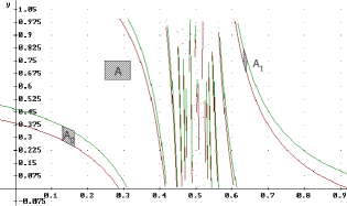
Figure 1: A small rectangle $A$ and $A_{0}$, $A_{1}$, its pre-images.

Figure 1 shows $A=[1/4,1/3]\times[2/3,3/4]$ and its pre-images, $A_{0}$ and $A_{1}$, where we have chosen $c=\pi-3\approx 0.1416$. The horizontal sides of $A$ are mapped into the broken graph of the hyperbolas, the top corresponding to the green line and the bottom to the red one.

Theorem 4.3.

Let $c>1/4$. Then the map $f$ is mixing with respect to Lebesgue measure.

Proof.

There is no loss of generality choosing $A$ and $R$ as rectangles contained in $Q$, since the family of rectangles generates the $\sigma$-algebra associated to the Lebesgue measure [Wa], Theorem 1.17. We have to show

$$\lim_{n\to\infty}|m(f^{-n}(A)\cap R)-m(A)\cdot m(R)|=0.$$

For this we proceed as follows. Let $W=(x^{R},y^{R})\in R$, be the center point of $R$ and $Z=(x^{A},y^{A})$ the center point of $A$. We use the binary decomposition of $x^{R}\sim b_{1}b_{2}\cdots$ and let $\hat{x}\sim\overline{b_{1}b_{2}\cdots b_{N}}=b,$ that is, $\hat{x}$ is the $N$-periodic point of the map $x\mapsto 2x$ mod $1$.

Taking $N$ sufficiently large, we have that the vertical line $x=\hat{x}$ crosses the rectangle $R$ nearby its central point $W$. Indeed, $|\hat{x}-x^{R}|<2^{-N}$. If $x_{{b}}=\Pi_{x}(Z_{{b}})$, as a consequence of the remarks after formula (2) we have $|x_{b}-\hat{x}|<2^{-N}$, and also $|x_{{b}}-x^{R}|<2^{-N}$.

Moreover, for $n\geq N$, with $N$ large enough, the $n$-th pre-image of any horizontal segment of length $\Delta x$ in $A$, is almost vertical and their length is greater than $2^{\lfloor n/N\rfloor}c\Delta x$, see Lemma 4.1.

Claim 4.1.

The distance $h_{a}$ between the pre-images of the top and the bottom of $A$ by $Z_{{a}}$, where $a=a_{1}a_{2}\cdots a_{n}$, see (2), is

$$h_{a}\approx\frac{m(A)}{2^{n}\cdot\Delta x_{A}\cdot}L_{a},$$ (4)

where $\Delta x_{A}$ is the length of the bottom of $A$ and $L_{a}>(4c)^{[n/N]}$.

Proof.

$Z_{{a}}(A)$ has measure equal to $m(A)/2^{n}$. Moreover, as a consequence of Lemma 4.1 the length $l_{a}$ of $\Pi_{x}(Z_{{a}}(A))$ is given by $\Delta x_{A}\cdot L_{a}$. Thus the height $h_{a}$ of the almost parallelogram given by $Z_{{a}}(A)$ is

$$h_{a}\approx\frac{m(A)}{2^{n}\cdot l_{a}}=\frac{m(A)}{2^{n}\cdot\Delta x_{A}\cdot L_{a}}$$

proving the claim. ∎

Returning to the proof of Theorem 4.3 note that if $n$ is large enough, as a consequence of the remarks after equations (a) and (b) at (2), $Z_{{a}}(A)$ is a long “vertical” strip almost uniformly distributed in the torus. Then there are $\Delta x_{A}L_{a}\Delta x_{R}$ strips cutting $R$. By claim 4.1 each turn leaves a strip in $R$ of area

$$\frac{\Delta y_{R}\cdot m(A)}{\Delta x_{A}\cdot 2^{n}\cdot L_{a}}.$$

Then the total area equals

$$\frac{\Delta y_{R}\cdot m(A)\cdot\Delta x_{A}\cdot L_{a}\cdot\Delta x_{R}}{\Delta x_{A}\cdot 2^{n}\cdot L_{a}}=\frac{\Delta y_{R}\cdot m(A)\cdot\Delta x_{R}}{2^{n}}.$$

Since the number of pre-images satisfying the previous computations is $2^{n}$ we obtain that

$$m(f^{-n}(A)\cap R)\approx\frac{M(R)\cdot m(A)}{2^{n}}\cdot 2^{n}\to m(A)\cdot m(R)\quad\mbox{for }\quad n\to\infty\,,$$

finishing the proof. ∎

Lemma 4.2 together with Theorem 4.3 prove Theorem B.

5 Rate of mixing

Next we prove that the rate of mixing for $c>1/4$ is exponential. To do so we start with an auxiliary lemma.

Lemma 5.1.

Given $b\in[0,1)$,

$$b=\frac{b_{1}}{2}+\frac{b_{2}}{2^{2}}+\cdots+\frac{b_{N-1}}{2^{N-1}}+\frac{b_{N}}{2^{N}}\sim b_{1}b_{2}\cdots b_{N-1}b_{N},$$

there is at most one point in $(0,1)$ where the derivative $y_{b}^{\prime}(x_{b})$ can vanish. Moreover, if $y_{b}^{\prime}(x_{b})$ vanishes, the value of $x$ at which $y^{\prime}_{b}=0$ is between $\Sigma_{i=1}^{j}b_{i}/2^{i}$ and $\Sigma_{i=1}^{j}b_{i}/2^{i}+1/2^{N}$ where $b_{j}$ is the first digit in $b_{1}b_{2}\cdots b_{N-1}b_{N}$ different from $b_{N}$ (i.e.: $b_{N}=b_{N-1}=\cdots=b_{j+1}\neq b_{j}$).

Proof.

We will repeatedly use that $y_{b}$ and $x_{b}$ are given by equations (a) and (b) at (2). Let $(x_{0},y_{0})$ be given.

For $N=1$ we have that

$$y_{b_{1}}=y_{0}-\frac{c}{|x_{b_{1}}-1/2|}\mod(1)=y_{0}-\frac{c\cdot(2b_{1}-1)}{x_{b_{1}}-1/2}\mod(1)$$

where $x_{b_{1}}=\frac{x_{0}+b_{1}}{2}\in(\frac{b_{1}}{2},\frac{b_{1}+1}{2})$. Observe that $2b_{1}-1=-1$ if $b_{1}=0$ and $2b_{1}-1=1$ if $b_{1}=1$. Thus

$$y_{b_{1}}^{\prime}(x_{b_{1}})=\frac{c\cdot(2b_{1}-1)}{(x_{b_{1}}-1/2)^{2}}\quad\mbox{which does not vanish whenever it exists.}$$

For $N=2$, on account that

$$x_{b_{1}b_{2}}=\frac{x_{b_{2}}+b_{1}}{2}\in(\frac{b_{1}}{2}+\frac{b_{2}}{2^{2}},\frac{b_{1}}{2}+\frac{b_{2}}{2^{2}}+\frac{1}{2^{2}})$$

we have $x_{b_{2}}=2x_{b_{1}b_{2}}-b_{1}$ and

$$y_{b_{1}b_{2}}(x_{b_{1}b_{2}})=y_{b_{2}}-\frac{c}{|x_{b_{1}b_{2}}-1/2|}=y_{0}-\frac{c}{|x_{b_{2}}-1/2|}-\frac{c}{|x_{b_{1}b_{2}}-1/2|}\mod(1)=$$

$$=y_{0}-\frac{c\cdot(2b_{2}-1)}{(2x_{b_{1}b_{2}}-b_{1}-1/2)}-\frac{c\cdot(2b_{1}-1)}{(x_{b_{1}b_{2}}-1/2)}\mod(1)$$

from which we conclude that

$$y_{b_{1}b_{2}}^{\prime}(x_{b_{1}b_{2}})=\frac{2c\cdot(2b_{2}-1)}{(2x_{b_{1}b_{2}}-b_{1}-1/2)^{2}}+\frac{c\cdot(2b_{1}-1)}{(x_{b_{1}b_{2}}-1/2)^{2}}\,,$$

which does not change sign if $b_{1}=b_{2}$ or changes sign only once in its domain if $b_{1}\neq b_{2}$.

In general the expression of $y_{b}=y_{b_{1}b_{2}\cdots b_{N}}$ as a function of $x_{b}=x_{b_{1}b_{2}\cdots b_{N}}$ is given by

$$y_{b}(x_{b})=y_{0}-\frac{c\cdot(2b_{N}-1)}{(2^{N-1}x_{b}-(2^{N-2}b_{1}+2^{N-3}b_{2}+\cdots+2b_{N-2}+b_{N-1})-1/2)}\,-$$

$$\frac{c\cdot(2b_{N-1}-1)}{(2^{N-2}x_{b}-(2_{N-3}b_{1}+2^{N-4}b_{2}+\cdots+2b_{N-3}+b_{N-2})-1/2)}-\cdots-\frac{c\cdot(2b_{1}-1)}{(x_{b}-1/2)}\mod(1)$$

from which the derivative of $y_{b}$ with respect to $x_{b}$, whenever it exists, is given by

$$y_{b}^{\prime}(x_{b})=\frac{2^{N-1}c\cdot(2b_{N}-1)}{(2^{N-1}x_{b}-(2_{N-2}b_{1}+2^{N-3}b_{2}+\cdots+2b_{N-2}+b_{N-1})-1/2)^{2}}\,+$$

$$\frac{2^{N-2}c\cdot(2b_{N-1}-1)}{(2^{N-2}x_{b}-(2_{N-3}b_{1}+2^{N-4}b_{2}+\cdots+2b_{N-3}+b_{N-2})-1/2)^{2}}+\cdots+\frac{c\cdot(2b_{1}-1)}{(x_{b}-1/2)^{2}}\,.$$

The last expression can be written as

$$y_{b}^{\prime}(x_{b})=\frac{c\cdot(2b_{N}-1)}{2^{N-1}\left(x_{b}-(\frac{b_{1}}{2}+\frac{b_{2}}{2^{2}}+\cdots+\frac{b_{N-2}}{2^{N-2}}+\frac{b_{N-1}}{2^{N-1}})-\frac{1}{2^{N}}\right)^{2}}\,+$$

$$\frac{c\cdot(2b_{N-1}-1)}{2^{N-2}\left(x_{b}-(\frac{b_{1}}{2}+\frac{b_{2}}{2^{2}}+\cdots+\frac{b_{N-3}}{2^{N-3}}+\frac{b_{N-2}}{2^{N-2}})-\frac{1}{2^{N-1}}\right)^{2}}+\cdots+\frac{c\cdot(2b_{1}-1)}{\left(x_{b}-\frac{1}{2}\right)^{2}}\,.$$

$$\mbox{Hence }\quad y_{b}^{\prime}(x_{b})=\frac{c\cdot(2b_{N}-1)}{2^{N-1}\left(x_{b}-0.b_{1}b_{2}\cdots b_{N-2}b_{N-1}-\frac{1}{2^{N}}\right)^{2}}\,+$$

$$\frac{c\cdot(2b_{N-1}-1)}{2^{N-2}\left(x_{b}-0.b_{1}b_{2}\cdots b_{N-3}b_{N-2}-\frac{1}{2^{N-1}}\right)^{2}}+\cdots+\frac{c\cdot(2b_{1}-1)}{\left(x_{b}-\frac{1}{2}\right)^{2}}\,$$

where we have written $\frac{b_{1}}{2}+\frac{b_{2}}{2^{2}}+\cdots+\frac{b_{N-2}}{2^{N-2}}+\frac{b_{N-1}}{2^{N-1}}=0.b_{1}b_{2}\cdots b_{N-1}$, and similarly for the other terms. Observe that each term in the expression or $y^{\prime}_{b}(x_{b})$ is positive or negative depending on the values of $b_{i}$ and that there are $N$ vertical asymptotes for (the lift to $\mbox{$I\!\!R$}^{2}$ of) $y_{b}(x_{b})$ and for $y^{\prime}_{b}(x_{b})$ which are located in

$$x=0.b_{1}b_{2}\cdots b_{N-1}+\frac{1}{2^{N}}\,,\quad x=0.b_{1}b_{2}\cdots b_{N-2}+\frac{1}{2^{N-1}}\,,\;$$ (5)

$$x=0.b_{1}b_{2}\cdots b_{N-3}+\frac{1}{2^{N-2}}\,,\quad\ldots\,,\quad x=0.b_{1}+\frac{1}{2^{2}}\,,\quad x=\frac{1}{2}\,.$$

Claim 5.1.

All the terms with positive sign in $y_{b}^{\prime}(x_{b})$ have their asymptotes at points of coordinates less than those which have negative sign. Moreover $y^{\prime}_{b}(x_{b})$ will vanish only once for an $x_{\xi}$ located between the closest asymptotes of different sign.

Proof.

Let us prove the claim by induction.

For $N=1$ there is nothing to prove. For $N=2$, if $b_{2}=0$ and $b_{1}=1$ then we have an asymptote $x=\frac{1}{2}$ and the other $x=\frac{3}{4}$ and the derivative is

$$y_{b_{1}b_{2}}^{\prime}(x_{b_{1}b_{2}})=y_{10}^{\prime}(x_{10})=\frac{-c}{2(x_{10}-3/4)^{2}}+\frac{c}{(x_{10}-1/2)^{2}}\,,$$

If $b_{2}=1$ and $b_{1}=0$ then we have an asymptote $x=1/4$ and the other $x=1/2$ and the derivative is

$$y_{b_{1}b_{2}}^{\prime}(x_{b_{1}b_{2}})=y_{01}^{\prime}(x_{01})=\frac{c}{2(x_{01}-1/4)^{2}}+\frac{-c}{(x_{01}-1/2)^{2}}\,.$$

Hence the claim is true for $N=1,\,2$.

Assume that the claim is true for $b_{2}b_{3}\cdots b_{N}$ and let us prove it for $b=b_{1}b_{2}b_{3}\cdots b_{N}$. If $b_{1}=0$ then all the values of the asymptotes are divided by 2 and the corresponding asymptotes of the positive terms in $y^{\prime}_{b}(x_{b})$ rest to the left of the smallest asymptote corresponding to a negative term (if there is any one). By induction the difference between the smallest asymptote of a negative term and the largest asymptote of a positive term is $1/2^{N-1}$ for $b_{2}b_{3}\cdots b_{N}$, when we divide by 2 the difference becomes $1/2^{N}$. Moreover, all terms are less than $1/2$ and we add a negative term corresponding to the asymptote $x=1/2$. Thus the claim is true for $b_{1}=0$.

If $b_{1}=1$ then all the values of the asymptotes are divided by 2 and to these values we add $1/2$. Therefore the corresponding asymptotes of the positive terms in $y^{\prime}_{b}(x_{b})$ rest to the left of the smallest asymptote corresponding to a negative term (if there is any). The difference between the smallest asymptote of a negative term and the largest asymptote of a positive term becomes $1/2^{N}$ as above. All terms are greater than $1/2$ and we add a positive term corresponding to the asymptote $x=1/2$.

If it were the case that $b_{2}=b_{3}=\cdots b_{N}=0$ but $b_{1}=1$, then all terms should be negative till the last one. After the final step a positive term appears with asymptote $x=1/2$ while the leftmost negative term will be $1/2+1/2^{N}$. Similarly if $b_{2}=b_{3}=\cdots b_{N}=1$ but $b_{1}=0$, then all terms should be positive till the last one. After the final step a negative term appears with asymptote $x=1/2$ while the rightmost positive term will be $1/2-1/2^{N}$. Now the proof of the claim is complete. ∎

The proof of the lemma follows readily from Claim 5.1, doing computations similar to those for the case $N=2$.

∎

Remark 5.2.

Although the number of asymptotes is $N$, since $x\in[0,1]$ we have that $x_{b}$ belongs to an interval of length $\frac{1}{2^{N}}$ and in the general case only two of the asymptotes fall in the domain of $x_{b}$. The distance between these asymptotes is $\frac{1}{2^{N}}$.

Remark 5.3.

Let $A=[x_{A}-\Delta x/2,x_{A}+\Delta x/2]\times[y_{A},y_{A}+\Delta y]$. From Lemma 4.1 it follows immediately that there is a first $N_{0}=N_{0}(\Delta x)$ such that $\ell(Z_{b}([x_{A}-\Delta x/2,x_{A}+\Delta x/2]))\geq 1$ if $|b|=N_{0}$.

The following lemma says that far from the asymptotes the growth of lengths of the pre-images is bounded from above.

Lemma 5.4.

Let $c>0$. Given $K>0$ and $\epsilon>0$ there is $\delta>0$ such that if $0<\Delta x\leq\delta$ then $N_{0}>K$ for a subset of $\Sigma$ of measure greater or equal than $1-K\epsilon$.

Proof.

Let us choose a vertical strip $S_{\epsilon}=[1/2-\epsilon/2,1/2+\epsilon/2]\times[0,1)$ and assume that $I=[x-\Delta x/2,x+\Delta x/2]\times\{y\}$ does not intersect $S_{\epsilon}$. Let us bound from above the length of the pre-images of $I$. Recall that these pre-images are given by

$Z_{0}=\left(\frac{x}{2},y-\frac{2c}{1-x}-\lfloor y-\frac{2c}{1-x}\rfloor\right)=(x_{0},y_{0})$ and

$Z_{1}=\left(\frac{1+x}{2},y-\frac{2c}{x}-\lfloor y-\frac{2c}{x}\rfloor\right)=(x_{1},y_{1}).$

Let us assume that $x+\Delta x/2<1/2-\epsilon/2$, the other cases are similar. This implies in particular that $1-x>\epsilon$. We obtain:

$$\ell(Z_{0}(I))=\int_{x/2-\Delta x/2}^{x/2+\Delta x/2}\sqrt{1+\frac{c^{2}}{(1/2-s)^{4}}}ds=$$

$$\int_{x/2-\Delta x/2}^{x/2+\Delta x/2}\left(\frac{(1/2-s)^{4}+c^{2}}{(1/2-s)^{4}}\right)^{1/2}ds\leq\int_{x/2-\Delta x/2}^{x/2+\Delta x/2}\frac{(1/16+c^{2})^{1/2}}{(1/2-s)^{2}}ds\leq$$

$$\left.\frac{c+1/4}{1/2-s}\right|_{(x-\Delta x)/2}^{(x+\Delta x)/2}=\frac{2c+1/2}{1-x}\left[\frac{1}{1-\Delta x/(1-x)}-\frac{1}{1+\Delta x/(1-x)}\right]=$$

$$\frac{2c+1/2}{(1-x)^{2}}2\Delta x\left[1+\frac{(\Delta x)^{2}}{(1-x)^{2}}+\frac{(\Delta x)^{4}}{(1-x)^{4}}+\cdots\right]<\frac{2c+1/2}{\epsilon^{2}}\left(\frac{1}{(1-\delta^{2}/\epsilon^{2})}\right)2\delta$$

where we have put $\Delta x<\delta<\epsilon$. This gives the upper bound for the length of a pre-image given by

$$\ell(Z_{0}(I))<\frac{4c+1}{\epsilon^{2}-\delta^{2}}\delta$$

The same bound is valid for the case $x>1/2$ and for the other pre-image given by $Z_{1}$.

Let us denote by $b^{(K)}=b_{1}b_{2}b_{3}\cdots b_{K}$ the finite subsequence given by the first $K$ terms of $b=\{b_{n}\}_{n\in\mbox{$I\!\!N$}}\in\Sigma$ and

$$X_{K}(x,y)=\{(x_{b^{(K)}},y_{b^{(K)}})\,:\,f^{K}(x_{b^{(K)}},y_{b^{(K)}})=(x,y)\}\,.$$

There is $\epsilon>0$ such that if $f^{j}([u-\Delta x/2,u+\Delta x/2],v)\cap[1/2-\epsilon/2,1/2+\epsilon/2]\times[0,1)=\emptyset$ for all $j=0,1,2,\ldots,K-1$ then the length of $Z_{b^{(K)}}(([u-\Delta x/2,u+\Delta x/2],v))<\left(\frac{4c+1}{\epsilon^{2}-\delta^{2}}\delta\right)^{K}$ from which the thesis follows choosing $\delta$ small enough.

∎

By Remark 5.3 after $N_{0}$ iterations the length of $Z_{b^{(N_{0})}}$ is at least 1. Thus if $k_{0}$ denotes the time needed for a monotone arc $\gamma$ to duplicate its length when computing $Z_{(b)^{(k_{0})}}$ (see Lemma 4.1) we obtain the following

Corollary 5.5.

If $N=N_{0}+k_{0}h$, $h\geq 0$, then for $b$ such that $|b|=N$ we have that

$$\ell(Z_{b}([x_{A}-\Delta x/2,x_{A}+\Delta x/2]\times\{y\}))\geq 2^{h}.$$

Corollary 5.5 implies that the pre-image $Z_{b}(A)$ has $2^{h}$ connected components in $[0,1]\times[0,1]$ which are almost vertical strips. The value of $N_{0}$ is bounded but depends on the length of $\Delta x$ and the position of $x_{A}$.

The next lemma estimates the width of each of these strips. Before we state it, let us sort out the intersections between $Z_{b}(A)$ and $[0,1]\times[0,1]$ in the following way:

$(\star)$ The image in $\mbox{$I\!\!R$}^{2}$ of the top side $T=[x_{A}-\Delta x/2,x_{A}+\Delta x/2]\times\{y+\Delta y\}$ of $A$ is an arc almost parallel to the vertical axis $Oy$ with reverse orientation. We assign the label $n$ to the connected component of this arc whose projection covers the interval $[-n+1,-n]$ in $Oy$ (see Figures 2 and 3). Similarly for the bottom segment $B=[x_{A}-\Delta x/2,x_{A}+\Delta x/2]\times\{y\}$.

Figure 2: The image of $T$ in $\mbox{$I\!\!R$}^{2}$.

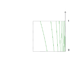
Figure 3: The image of $T$ in $[0,1]\times[0,1]$.

Lemma 5.6.

Let $A=[x_{A}-\Delta x/2,x_{A}+\Delta x/2]\times[y_{A},y_{A}+\Delta y]$ and $N=N_{0}+k_{0}\,h$, $h\geq 0$, be as above. Denote by $T$ the top and $B$ the bottom sides of the rectangle $A$. Then, for $b$ such that $|b|=N$ there is a constant $C>0$ such that

$${\rm dist}(Z_{b}(T)_{n},Z_{b}(B)_{n})\leq C\frac{\Delta y}{2^{N}n^{2}}\,,$$

where $Z_{b}(T)_{n}$, and $Z_{b}(B)_{n}$ are the $n^{th}$-connected component of $Z_{b}(T)$ and $Z_{b}(B)$ respectively.

Proof.

For the bottom side $B$ the expression of $y_{b}=y_{b_{1}b_{2}\cdots b_{N}}$ in $\mbox{$I\!\!R$}^{2}$ as a function of $x_{b}=x_{b_{1}b_{2}\cdots b_{N}}$ is given by (see the proof of Lemma 5.1)

$$y_{b}(x_{b})=y_{A}-\frac{c\cdot(2b_{N}-1)}{(2^{N-1}x_{b}-(2^{N-2}b_{1}+2^{N-3}b_{2}+\cdots+2b_{N-2}+b_{N-1})-1/2)}\,-$$

$$\frac{c\cdot(2b^{N-1}-1)}{(2^{N-2}x_{b}-(2{N-3}b_{1}+2^{N-4}b_{2}+\cdots+2b_{N-3}+b_{N-2})-1/2)}-\cdots-\frac{c\cdot(2b_{1}-1)}{(x_{b}-1/2)}\,.$$

This curve has $N$ asymptotes $x_{1},x_{2},\ldots,x_{N}$, see equation (5). Close to one of each asymptotes, say $x_{b}=x_{j}$, $y_{b}(x_{b})$ can be written as

$$y_{b}(x_{b})=y_{A}+H(x_{b})+\frac{c\,(2b_{j}-1)/2^{j-1}}{(x_{b}-x_{j})}\,,\quad$$

where $H(x_{b})$ has a finite limit $H_{j}$ when $x_{b}\to x_{j}$. Similarly for the top side $T$ we have

$$y_{b}(x_{b})=y_{A}+\Delta y+H(x_{b})+\frac{c\,(2b_{j}-1)/2^{j-1}}{(x_{b}-x_{j})}\,.\quad$$

The only values that give asymptotes in the domain of $x_{b}$ correspond to the case $j=N$ that give

$$y_{b}(x_{b})=y_{A}+H(x_{b})+\frac{c\,(2b_{N}-1)/2^{N-1}}{(x_{b}-x_{N})}\,,\quad$$

and

$$y_{b}(x_{b})=y_{A}+\Delta y+H(x_{b})+\frac{c\,(2b_{N}-1)/2^{N-1}}{(x_{b}-x_{N})}\,.\quad$$

For a fixed $y_{b}$, varying from $-n+1$ to $-n$, we have

$$(\star_{1})\,\,y_{b}=y_{A}+H(\tilde{x}_{b})+\frac{c\,(2b_{N}-1)/2^{N-1}}{(\tilde{x_{b}}-x_{N})}\quad\mbox{and}\quad(\star_{2})\,\,y_{b}=y_{A}+\Delta y+H(\widehat{x_{b}})+\frac{c\,(2b_{N}-1)/2^{N-1}}{(\widehat{x_{b}}-x_{N})}\,.$$

For a given $\varepsilon>0$, there is $n_{0}$ such that for $n>n_{0}$ it holds that $|H(x_{b})-H_{N}|<\varepsilon$. Thus, from the first equation $(\star_{1})$ we have that, for $n>n_{0}$, it holds

$$y_{b}\approx y_{A}+H_{N}+\frac{c\,(2b_{N}-1)/2^{N-1}}{(\tilde{x}_{b}-x_{N})}\Longrightarrow\tilde{x}_{b}\approx x_{N}+\frac{c(2b_{N}-1)}{(y_{b}-y_{A}-H_{N})2^{N-1}}\,.$$

From the second one $(\star_{2})$ we obtain that

$$y_{b}\approx y_{A}+H_{N}+\Delta y+\frac{c\,(2b_{N}-1)/2^{N-1}}{(\widehat{x}_{b}-x_{N})}\Longrightarrow\widehat{x}_{b}\approx x_{N}+\frac{c(2b_{N}-1)}{(y_{b}-y_{A}-H_{N}-\Delta y)2^{N-1}}\,.$$

This implies that

$$|\widehat{x}_{b}-\tilde{x}_{b}|\approx\left|\frac{c(2b_{N}-1)}{(y_{b}-y_{A}-H_{N}-\Delta y)2^{N-1}}-\frac{c(2b_{N}-1)}{(y_{b}-y_{A}-H_{N})2^{N-1}}\right|\,.$$

Taking into account that $-n+1>y_{b}>-n$ and $2b_{N}-1=\pm 1$ we conclude that

$$|\widehat{x}_{b}-\tilde{x}_{b}|\approx\frac{c}{2^{N-1}}\left(\frac{1}{(-n-y_{A}-H_{N}-\Delta y)}-\frac{1}{(-n-y_{A}-H_{N})}\right)=$$

$$\frac{c}{2^{N-1}}\frac{\Delta y}{(n+y_{A}+H_{N})(n+y_{A}+H_{N}+\Delta y)}<\frac{c}{2^{N-1}}\frac{\Delta y}{n^{2}}<C\frac{\Delta y}{2^{N}n^{2}}\,.$$

Here we have chosen the constant $C>0$ such that the inequality holds for all $n\geq 1$ and not only for $n>n_{0}$. ∎

Theorem 5.7.

There is $0<\theta<1$ such that after $N=N_{0}+k_{0}\,h$ iterates by any branch $Z_{b}$ of $f^{-1}$, the Lebesgue measure of the set of points that has returned to $A$ is greater or equal to $m(A)\cdot\theta$.

Proof.

Let $\ell(Z_{b}([x_{A}-\Delta x/2,x_{A}+\Delta x/2]\times\{y\}))=2^{h}$ with $|b|=N$ (Corollary 5.5), and assume that $\Pi_{x}(Z_{b}(x_{a},y)\in[x_{A}-\Delta x/2+\frac{1}{2^{N}},x_{A}+\Delta x/2-\frac{1}{2^{N}}]$. Then $Z_{b}(A)$ cuts $A$ in at least $2^{h}$ strips which are almost vertical except perhaps for one which becomes from that strip where the derivative $y_{b}^{\prime}(x_{b})$ can vanish. We don’t take into account this strip so that we either have $2^{h}$ almost vertical strips or $(2^{h}-1)$ of them. Since $2^{h}$ is a lower bound we will consider that the number of strips is $2^{h}$ anyway. By Lemma 5.6 the (almost) vertical sides of the strips which are at a distance between them $\approx\frac{C\Delta y}{2^{N}n^{2}}$ intersected with $A$ are mapped by $f^{N}$, $N=|b|$, in part of the horizontal sides of length proportional to $C\Delta y/n^{2}$ with $N_{0}\leq n\leq 2^{h}$. Thus the area covered by the $f^{N}$-image of one of the strips is about a constant $D$ multiplied by the length $\Delta y/n^{2}$ of the horizontal sub-intervals, by the height $\Delta y$ which gives

$$\mbox{Area}_{n}\approx D\cdot\frac{\Delta y}{n^{2}}\cdot\Delta y\,.$$

It follows that the area of the $f^{N}$-image of the $2^{h}$strips is

$$\sum_{n=N_{0}}^{2^{h}}\mbox{Area}_{n}=D\cdot(\Delta y)^{2}\sum_{n=N_{0}}^{2^{h}}\frac{1}{n^{2}}\,.$$

Since any point in $A$ has $2^{N}$ preimages by the different $Z_{b}$, $|b|=N$, we have to divide this number by $2^{N}$ in order not to multiple count. This gives us

$$D\cdot(\Delta y)^{2}\frac{\sum_{n=N_{0}}^{2^{h}}\frac{1}{n^{2}}}{2^{N}}\,.$$

Since the number of preimages from $N_{0}$ to $N$ that cut $A$ is given by the action of $x\mapsto 2x\mod(1)$ in $[0,1)$, which is Bernoulli, we have that this number is $\approx 2^{k_{0}h}\Delta x$. Hence we have that the area of the set of points that have returned after $N$ preimages is

$$\mbox{covered area}\approx D\cdot(\Delta y)^{2}\frac{\sum_{n=N_{0}}^{2^{h}}\frac{1}{n^{2}}}{2^{N}}\Delta x\cdot 2^{k_{0}h}=\Delta x\Delta y\left(D\cdot\Delta y\cdot\frac{2^{k_{0}h}}{2^{N_{0}+k_{0}h}}\cdot\sum_{n=N_{0}}^{2^{h}}\frac{1}{n^{2}}\right)=$$

$$=m(A)\left(D\cdot\Delta y\cdot 2^{-N_{0}}\cdot\sum_{n=N_{0}}^{2^{h}}\frac{1}{n^{2}}\right)=m(A)\cdot\theta,\,$$

$$\mbox{where}\quad\theta=D\cdot\Delta y\cdot 2^{-N_{0}}\cdot\sum_{n=N_{0}}^{2^{h}}\frac{1}{n^{2}}<1\,.$$

Therefore the measure of the set of points that have not returned yet is at most $m(A)(1-\theta)$. After taking $2^{N}$ new preimages (i.e.: by backward iteration $N$ times following all the possible $2^{N}$ branches $Z_{b}$, $|b|=N$, from the new starting point) we cover $m(A)(1-\theta)\theta$ which implies that it rests at most $m(A)(1-\theta)^{2}$ points that have not returned to $A$ yet. We conclude by induction that for $|b|=nN$ the measure of points not covered after taking all $2^{nN}$ pre-images is less than $m(A)(1-\theta)^{n}\to 0$ when $n\to\infty$. ∎

Corollary 5.8.

We have that after $n\,N$ iterates, the Lebesgue measure of points that have not yet returned is less than $m(A)(1-\theta)^{n}$.

The next corollary gives that the rate of recurrence of $f$ is exponential.

Corollary 5.9.

It holds that $\lim_{n\to\infty}|m(f^{-n}(A)\cap A)-m^{2}(A)|=0$ exponentially fast.

Proof.

Note that by Theorem 5.7 we have that the measure of points that have returned to $A$ after $N$ iterations is

$$m(A)\left(D\cdot\Delta y\cdot 2^{-N_{0}}\cdot\sum_{n=N_{0}}^{2^{h}}\frac{1}{n^{2}}\right)\,.$$

We may write this expression as

$$m(A)\left(D\cdot\Delta x\cdot\Delta y\cdot\frac{2^{-N_{0}}}{\Delta x}\cdot\sum_{n=N_{0}}^{2^{h}\Delta x}\frac{1}{n^{2}}\right)=(m(A))^{2}\left(D\cdot\frac{2^{-N_{0}}}{\Delta x}\cdot\sum_{n=N_{0}}^{2^{h}\Delta x}\frac{1}{n^{2}}\right)\,.$$

For $N_{0}$ sufficiently large we have that $\lambda=\left(D\cdot\frac{2^{-N_{0}}}{\Delta x}\cdot\sum_{n=N_{0}}^{n=2^{h}}\frac{1}{n^{2}}\right)<1$ and therefore we obtain that after $n=hN$ iterations

$$|m(f^{-n}(A)\cap A)-m^{2}(A)|\leq|(m(A))^{2}\big{(}1-\lambda^{\left[\frac{n;}{N}\right]}\big{)}-(m(A))^{2}|=(m(A))^{2}\lambda^{\left[\frac{n}{N}\right]}$$

Putting $\lambda^{1/N}=\tau<1$ we have

$$|m(f^{-n}(A)\cap A)-m^{2}(A)|\leq(m(A))^{2}\tau^{n}$$

proving the thesis. ∎

The following theorem is similar to Theorem 5.7.

Theorem 5.10.

Given small rectangles $A=[x_{A}-\frac{\Delta x_{A}}{2},x_{A}+\frac{\Delta x_{A}}{2}]\times[y_{A},y_{A}+\Delta y_{A}]$ and $B=[x_{B}-\frac{\Delta x_{B}}{2},x_{B}+\frac{\Delta x_{B}}{2}]\times[y_{B},y_{B}+\Delta y_{B}]$ there is $0<\theta<1$ such that the set of points of $A$ that has visited $B$ after $N$ iterates is greater or equal than $m(B)\cdot\theta$.

Proof.

By Corollary 5.5 we have that $\ell(Z_{b}([x_{A}-\frac{\Delta x_{A}}{2},x_{A}+\frac{\Delta x_{A}}{2}]\times\{y\}))=2^{h}$ with $|b|=N$. Assume that $\Pi_{x}(Z_{b}(x_{a},y))\in[x_{B}-\frac{\Delta x_{B}}{2}+\frac{1}{2^{N}},x_{B}+\frac{\Delta x_{B}}{2}-\frac{1}{2^{N}}]$. Then $Z_{b}(A)$ cuts $B$ in $2^{h}$ strips which are almost vertical except perhaps for one of them corresponding to that strip where the derivative $y_{b}^{\prime}(x_{b})$ vanishes. We don’t take into account this strip so that we either have $2^{h}\Delta x_{A}$ or $(2^{h}-1)\Delta x_{A}$ almost vertical strips. The area of $Z_{b}(A)$ is $m(A)/2^{N}$.

By Lemma 5.6 and taking into account the sorting given at $(\star)$, the intersection of the (almost) vertical sides of the strips with $B$ are mapped by $f^{N}$, $N=|b|$, in a subsegment of the horizontal sides of $A$ with length $\approx C\Delta y_{B}/n^{2}$, $N_{0}\leq n\leq 2^{h}$, recall Corollary 5.5.

Thus, the area covered by the $f^{N}$-image of the $n^{th}$-strip is given by

$$(\mbox{Area in }A)_{n}\approx D\cdot\frac{\Delta y_{B}}{n^{2}}\cdot\Delta y_{A}\,,$$

where $D$ is a constant, $\Delta y_{B}$ is the length of the vertical side of $B$, and $\Delta y_{A}$ is the length of the vertical side of $A$.

Therefore, the area of the $f^{N}$-image of all the $(2^{h}-N_{0})$ strips is

$$\sum_{n=N_{0}}^{2^{h}}\mbox{Area}_{n}=D\cdot(\Delta y_{A})(\Delta y_{B})\sum_{n=N_{0}}^{2^{h}}\frac{1}{n^{2}}\,.$$

Since any point in $A$ has $2^{N}$ pre-images by the different $Z_{b}$, $|b|=N$, we have to divide this number by $2^{N}$ in order not to multiple count. This gives us

$$D\cdot(\Delta y_{A})(\Delta y_{B})\frac{\sum_{n=N_{0}}^{2^{h}}\frac{1}{n^{2}}}{2^{N}}\,.$$

Since the number of pre-images from $N_{0}$ to $N=N_{0}+2^{k_{0}h}$ that cut $B$ is given by the action of $x\mapsto 2x\mod(1)$ in $[0,1)$, which is Bernoulli, we have that this number is $\approx 2^{k_{0}h}\Delta x_{B}$. Hence we have that the area of the set of points that have cut $B$ after $N$ pre-images is

$$\approx D\cdot(\Delta y_{A})(\Delta y_{B})\frac{\sum_{n=N_{0}}^{2^{h}\Delta x_{A}}\frac{1}{n^{2}}}{2^{N}}\Delta x_{B}\cdot 2^{k_{0}h}=\Delta x_{B}\Delta y_{B}\left(D\cdot\Delta y_{A}\cdot\frac{2^{k_{0}h}}{2^{N_{0}+k_{0}h}}\cdot\sum_{n=N_{0}}^{2^{h}}\frac{1}{n^{2}}\right)=$$

$$=m(B)\left(D\cdot\Delta y_{A}\cdot 2^{-N_{0}}\cdot\sum_{n=N_{0}}^{2^{h}}\frac{1}{n^{2}}\right)=m(B)\cdot\theta,\,$$

$$\mbox{where}\quad\theta=D\cdot\Delta y_{A}\cdot 2^{-N_{0}}\cdot\sum_{n=N_{0}}^{2^{h}\Delta x}\frac{1}{n^{2}}<1\,.$$

Therefore the measure of the set of points of $A$ that have not visited yet the set $B$ is at most $m(B)(1-\theta)$. After taking $2^{N}$ new pre-images (i.e.: by backward iteration $N$ times following all the possible $2^{N}$ branches $Z_{b}$, $|b|=N$, from the new starting point) we cover $m(B)(1-\theta)\theta$ which implies that it rests at most $m(B)(1-\theta)^{2}$ points that have not visited $B$ yet.

By induction we conclude that for $|b|=nN$ the measure of points not covered after taking all $2^{nN}$ pre-images is less than $m(B)(1-\theta)^{n}\to 0$ when $n\to\infty$. ∎

The following corollary, whose proof is similar to that of Corollary 5.9 gives that the rate of mixing is exponential and concludes the proof of Theorem C.

Corollary 5.11.

It holds that $\lim_{n\to\infty}|m(f^{-n}(A)\cap B)-m(A)m(B)|=0$ exponentially fast.

M. J. Pacifico: Instituto de Matemática, Universidade Federal do Rio de Janeiro, C. P. 68.530, CEP 21.945-970, Rio de Janeiro, RJ, Brazil.
E-mail: pacifico@im.ufrj.br .

R. Markarian: Instituto de Matemática y Estadística (IMERL), Facultad de Ingeniería, Universidad de la República, CC30, CP 11300, Montevideo, Uruguay.
E-mail: roma@fing.edu.uy.

J. Vieitez: Regional Norte, Universidad de la Republica, Rivera 1350, CP 50000, Salto, Uruguay.
E-mail: jvieitez@unorte.edu.uy.

References

[AP]
V. Araújo and M. J. Pacifico.
Three-dimensional flows, volume 53 of Ergebnisse der
Mathematik und ihrer Grenzgebiete. 3. Folge. A Series of Modern Surveys in
Mathematics [Results in Mathematics and Related Areas. 3rd Series. A Series
of Modern Surveys in Mathematics].
Springer, Heidelberg, 2010.
With a foreword by Marcelo Viana.
[Ba] V. Baladi, Positive transfer operators and decay of correlations (Adv. Ser. Nonlinear Dyn., vol. 16) World Scientific, New Jersey (2000).
[BP] L. Barreira and Ya. Pesin, Lectures on Lyapunov exponents and smooth ergodic theory, Proc.
Sympos. Pure Math. 69, 3 - 106 (2001).
[Bo] R. Bowen. Equilibrium states and the ergodic theory of Anosov diffeomorphisms, volume 470
of Lect. Notes in Math. Springer Verlag, (1975).
[BY] M. Benedicks, L.-S. Young, Markov extensions and decay of correlations for certain H�enon
maps, Astérisque 261 (2000), 13-56.
[Bu] Bunimovich, L.A.: On the ergodic properties of nowhere dispersing billiards. Commun.
Math. Phys. 65, 295-312 (1979)
[Ch] N. Chernov Decay of correlations and dispersing billiards, J. Statist. Phys. 94 (1999) 513 - 556.
[CM] Chernov, N. Markarian R. Theory of chaotic billiards, (2006).
[CY] N. Chernov & L.-S. Young. Decay of correlations for Lorentz gases and hard balls. Encyclopaedia of Mathematical Sciences
101, Springer-Verlag, (2000) 89 - 120
[Do] D. Dolgopyat, On decay of correlations in Anosov flows, Ann. of Math., 147, (1998), 357 - 390.
[GW]
J. Guckenheimer and R. F. Williams.
Structural stability of Lorenz attractors.
Publ. Math. IHES, 50:59–72, 1979.
[Lo]
E. N. Lorenz.
Deterministic nonperiodic flow.
J. Atmosph. Sci., 20:130–141, 1963.
[Ru] Ruelle D. Ergodic Theory of Dynamical Systems, Publ Math IHES, 50, 27 - 58, (1979).
[Si] Sinai, Ya.G.: Dynamical systems with elastic reflections. Russ. Math. Surv. 25:1, 137-189
(1970)
[Vi] Viana, M. Stochastic dynamics of deterministic systems, Lecture Notes Braz. Math Colloq, IMPA, Rio de Janeiro, (1997).
[Wa] P. Walters. An Introduction to Ergodic Theory. Graduate Texts in Mathematics 79, Springer-Verlag, New York-Berlin, 1982. ix+250 pp.
[Yo1] L.-S. Young, Statistical properties of dynamical systems with some hyperbolicity, Ann. Math.
147 (1998), 585-650.
[Yo2] L.-S. Young, Recurrence times and rates of mixing, Israel J. Math. 110 (1999), 153-188.