CONVEX GEOMETRY: a travel to the limits of our knowledge

Abstract

Our knowledge and ignorance concerning the geometry of quantum states are discussed.

Questions about the structure

Physical theories are usually created by accumulating some fragments of information which at the beginning do not allow to predict the final structures. The classical mechanics was formulated by Isaac Newton in terms of mass, force, acceleration and the three dynamical laws. It was not immediate to see the Lagrangians, Hamilton equations and the simplectic geometry behind. We cannot guess the reaction of Newton if he were informed that he was just describing the classical phase spaces defined by the simplectic manifolds…

Quite similarly, Max Planck, Niels Bohr, Louis de Broglie, Erwin Schrödinger and Werner Heisenberg could not see from the very beginning that the physical facts which they described would be reduced by Born’s statistical interpretation to the Hilbert space geometry (as it seems, neither Hilbert could predict that). Yet, once accepted that the pure states of a quantum system can be represented by vectors of a complex linear space and the expectation values are just quadratic forms, the Hilbert spaces entered irremediably into the quantum theories. Together appeared the “density matrices” as the mathematical tools representing either pure or mixed quantum ensembles. Their role is now so commonly accepted that its origin is somehow lost in some petrified parts of our subconsciousness: an obligatory element of knowledge which the best university students (and the future specialists) learn by heart. However, is it indeed necessary? Can indeed the interference pictures of particle beams limit the fundamental quantum concepts to vectors in linear spaces and “density matrices”?

Quantum logic?

The desire to find some deeper reasons led a group of authors to postulate the existence of an “intrinsic logic” of quantum phenomena, called the quantum logic rf1 ; rf2 ; rf3 . Generalizing the classical ideas, it was understood as the collection $Q$ of all statements (informations) about a quantum object, possible to check by elementary “yes-no measurements”. Following the good traditions, $Q$ should be endowed with implication ($\Rightarrow$), and negation $a\rightarrow a^{\prime}$. The implication defines the partial order in $Q$ ($a\Rightarrow b$ reinterpreted as $a\leq b$), suggesting the next axioms about the existence of the lowest upper bound $a\lor b$ (“or” of the logic) and the greatest lower bound $a\wedge b$ (“and” of the logic) for any $a,b\in Q$. The “negation” was assumed to be involutive, $a^{\prime\prime}\equiv a$, satisfying de Morgan law: $(a\lor b)^{\prime}\equiv a^{\prime}\wedge b^{\prime}$ as well as other axioms granting that $Q$ is an orthocomplemented lattice rf1 . Until now, the whole structure looked quite traditional. With one exception: in contrast to the classical measurements, the quantum ones do not commute, which traduces itself into breaking the distributive law $(a\lor b)\wedge c\neq(a\wedge c)\lor(b\wedge c)$ obligatory in any classical logic. The quantum logic was non-Boolean! An intense search for an axiom which would generalize the distributive law, admitting both classical and quantum measurements, in agreement with Birkhoff, von Neumann, Finkelstein rf1 ; rf2 ; rf3 and thanks to the mathematical studies of Varadarajan rf4 convinced C. Piron to propose the weak modularity as the unifying law. To some surprise, the subsequent theorems rf4 ; rf5 exhibit certain natural completeness: the possible cases of “quantum logic” are exhausted by the Boolean and Hilbertian models, or by combinations of both. As pointed out by many authors this gives the theoretical physicists some reasonable confidence that the formalism they develop (with Hilbert spaces, density matrices, etc.) does not overlook something essential, so there will be no longer need to think too much about abstract foundations.

However, isn’t this confidence a bit too scholastic? It can be noticed that the general form of quantum theory, since a long time, is the only element of our knowledge which does not evolve. While the “quantization problem” is formulated for the existing (or hypothetical) objects of increasing dimension and flexibility (loops, strings, gauge fields, submanifolds or pseudo-Riemannian spaces, non-linear gravitons, etc.), the applied quantum structure is always the same rigid Hilbertian sphere or density matrix insensitive to the natural geometry of the “quantized” systems. The danger is that (in spite of all “spin foams”) we shall invest a lot of effort to describe the relativistic space-times in terms of the perfectly symmetric, “crystalline” forms of Hilbert spaces, like rigid bricks covering a curved highway. Is there any other option?…

Convex geometry

The alternatives arise if one decides to describe the statistical theories in terms of geometrical instead of logical concepts. What is the natural geometry of the statistical theory? It should describe the pure or mixed particle ensembles (also ensembles of multiparticle systems, including the mesoscopic or macroscopic objects). Suppose that one is not interested in the total number of the ensemble individuals, but only in their “average properties”. Two ensembles with the same statistical averages cannot be distinguished by any statistical experiments: we thus say that they define the same state. Now consider the set $S$ of all states for certain physical objects. Even in absence of any analytic description, there must exist in $S$ some simple empirical geometry. Given any two states $x_{1},x_{2}\in S$ (corresponding to certain ensembles $\mathcal{E}_{1}$, $\mathcal{E}_{2}$) and two numbers $p_{1},p_{2}\geq 0$, $p_{1}+p_{2}=1$, consider a new ensemble $\mathcal{E}$ formed by choosing randomly the objects of $\mathcal{E}_{1}$ and $\mathcal{E}_{2}$ with probabilities $p_{1}$ and $p_{2}$; its state, denoted $x=p_{1}x_{1}+p_{2}x_{2}$ is the mixture of $x_{1}$ and $x_{2}$ in proportions $p_{1},p_{2}$. If in turn both $x_{1},x_{2}$ are mixtures of $y_{1},y_{2}\in S$, then some more information is needed to determine the contents of $y_{1}$ and $y_{2}$ in $x$. It can be most simply expressed by representing $S$ as a subset of a certain affine space $\Gamma$, where $p_{1}x_{1}+p_{2}x_{2}$ becomes a linear combination. For any two points $x_{1},x_{2}\in S$ all mixtures $p_{1}x_{1}+p_{2}x_{2}$ ($p_{1},p_{2}\geq 0$, $p_{1}+p_{2}=1$) form then the straight line interval between $x_{1}$ and $x_{2}$, contained in $S$. Hence, $S$ is a convex set rf6 ; rf7 . To describe the limiting transitions, $\Gamma$ must possess a topology and $S$ should be closed in $\Gamma$.

The information encoded in the convex structure of $S$ might seem poor: it tells only which states are mixtures of which other states (see Fig. 1). Yet it turns out that it contains all essential information about both, logical and statistical aspects of quantum theory.

Figure 1: A convex set in 2D. Supposing that it could represent the states of some hypothetical ensembles, all border points except the straight line interval joining $x_{1}$ and $y_{1}$ would represent the pure states. All points in the interior are mixed states and do not allow a unique definition of the pure components. Thus, e.g., the state $z$ could be represented as a mixture of $x_{1}$ and $x_{2}$ or $y_{1}$ and $y_{2}$ or in any other way.

Logic of properties

The boundary of $S$ contains some special points $x$, which are not untrivial combinations $p_{1}x_{1}+p_{2}x_{2}$ with $p_{1},p_{2}>0$ of any two different points $x_{1}\neq x_{2}$ of $S$. These points, called extremal, represent the physical ensembles which are not mixtures of different components, and so are called pure. All subensembles of a pure ensemble define the same pure state $x$, which therefore represents also the quality of each single ensemble individual.

The convex geometry permits to describe as well more general ensemble properties which might be attributed to the single individuals. Note that, in general, the property of ensemble is not shared by the individuals (e.g., a human ensemble can contain 50% of men and 50% of women, but each individual, in general, has only one of these qualities). We say that the subset $P\subset S$ defines a property of the single objects if: 1. it resists mixing, i.e., $y_{1},y_{2}\in P$, $p_{1},p_{2}\geq 0$, $p_{1}+p_{2}=1$ $\Rightarrow$ $p_{1}y_{1}+p_{2}y_{2}\in P$ (meaning that $P$ is a convex subset of $S$), 2. if the property of mixture is shared by every mixture components, i.e., $y\in P$ and $p_{1}y_{1}+p_{2}y_{2}$, $y_{1},y_{2}\in S$, $p_{1},p_{2}>0\Rightarrow y_{1},y_{2}\in P$. The subset $P\subset S$ which satisfies 1. and 2. is called a face of $S$. The whole $S$ and the empty set $\emptyset$ are the improper faces: all other are plane fragments of various dimensionalities on the boundary of $S$ (See Fig. 2). In particular, each extremal points is a one point face. In what follows, we shall be most interested in the topologically closed faces of $S$ representing the “continuous properties” of the ensemble objects. Further on by faces we shall mean closed faces. Their whole family $\mathcal{P}$ admits a partial ordering $\leq$ identical with the set theoretical inclusion: the relation $P_{1}\leq P_{2}\Leftrightarrow P_{1}\subset P_{2}$ means that the property $P_{1}$ is more restrictive than $P_{2}$, or $P_{1}$ implies $P_{2}$. As easily seen, the intersection of any family of faces is again a face of $S$. Hence, for any two faces $P_{1},P_{2}\subset S$ there exists also their smallest upper bound, or union $P_{1}\lor P_{2}$, defined as the intersection of all faces containing both $P_{1}$ and $P_{2}$. The set $\mathcal{P}$ with the partial order $\leq$ (i.e., implication) and operations $\lor$, $\wedge$ is thus a complete lattice generalizing the “quantum logic” of the orthodox quantum mechanics: it might be called the logic of properties. We shall see that it does not necessarily include negation, but it admits a natural concept of orthogonality rf6 ; rf8 .

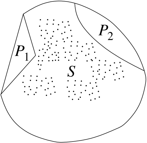
Figure 2: “Faces” on the border of $S$ represent properties of the single ensemble individuals. The picture in perspective permits to see that $P_{1}$ and $P_{2}$ are not orthogonal.

Counters

A natural counterpart of quantum ensembles are the measuring devices and the simplest such devices are particle counters. By a counter we shall understand any macroscopic body sensitive (either perfectly or partly) to the presence of quanta. Our assumption is also, that each counter reacts only to the properties of each single ensemble individual, without depending on the the rest. In mathematical terms, each counter can be described by a certain functional $\phi:S\rightarrow[0,1]$. whose values $\phi x$ for any $x\in S$ mean the fraction of particles in the state $x$ detected by the counter $\phi$. If $\phi x=1$, then the counter $\phi$ detects perfectly all $x$-particles, if $0<\phi x<1$, it overlooks a part, but if $\phi x=0$, then $\phi$ is completely blind to the $x$-particles. Moreover, if $\phi$ reacts only to single ensemble individuals, then for any mixed state $x=p_{1}x_{1}+p_{2}x_{2}$ it will detect independently both mixture components: $\phi x=p_{1}\phi x_{1}+p_{2}\phi x_{2}$, meaning that $\phi$ is a linear functional on $S$. We shall assume, that the values of counters permit to distinguish the different points $x\in S$ and moreover, they induce a physically meaningful topology, in which they are eo ipso continuous. Each continuous, linear functional $\phi$ taking on $S$ the values $0\leq\phi x\leq 1$ will be called normal. Mathematically, the counters are, therefore, the normal functionals. To get their geometric image, assume that the surrounding affine space $\Gamma\supset S$ is spanned by $S$. Hence, every linear functional $\phi$ on $S$ defines a unique linear functional on $\Gamma$ which will be denoted by the same symbol $\phi$. If $\phi\equiv\text{const.}$ on $S$, then $\phi\equiv\text{const.}$ on $\Gamma$. If not, then the equations $\phi x=c$, ($c\in\mathbb{R}$) split $\Gamma$ into a continuum of parallel hyperplanes on which $\phi$ accepts distinct constant values. Due to the linearity, $\phi$ is completely defined by the pair of hyperplanes on which it takes the values 0 and 1. If $\phi$ is normal, $S$ is contained in the closed belt of space between both planes. The question arises, how ample is the set of physical counters? Since no restrictions are evident, we shall assume that each normal functional represents a particle counter which at least in principle can be constructed. All distinct ways of counting particles can be thus read from the convex geometry of $S$ rf8 . They turn out closely related with the collection of hyperplanes and those are related with faces. Indeed, the hyperplanes $\phi=1$ and $\phi=0$ of a counter do not cross the interior of $S$, but can “touch” its boundary. As one can easily show, their common parts with the border $\partial S$ are two “opposite” faces (properties) of $S$, which awake completely different reactions of the counter: while detecting all particles on one of them, it ignores completely the particles on the other. Any two faces $P_{1}$, $P_{2}$, for which there exists at least one, so sharply discriminating counter, will be called excluding or orthogonal $(P_{1}\perp P_{2})$. The “logic of properties”, therefore, is a lattice with the relations of inclusion $(\leq)$ and exclusion $(\perp)$ though without a unique ortho-complement (since for any $P\in\mathcal{P}$, amongst all elements orthogonal to $P$ no greatest one must exist).

Detection ratios

Apart from orthogonality, the next geometry element of $S$ describes the selectivity limits of quantum measurements. Given a pair of pure states $x,y\in S$, consider the family of all counters $\phi$ detecting unmistakeably all particles of the state $x$, i.e., $\phi x=1$. Can they ignore completely the particles of the state $y$? In general, the answer is negative. The following lower bound over the counters $\phi$:

$$y:x=\operatorname{inf}_{\phi x=1}\phi y$$ (1)

called the “detection ratio” rf8 , if non-vanishing, describes a minimal fraction of $y$-particles which must infiltrate any experiment programmed to detect the $x$-state. The geometric character of this quantity is defined just by convex structure of $S$, which determines the support planes (see Fig. 3).

Figure 3: The could be convex set $S$ for some hypothetical ensembles. The parallel support lines $\chi=1$ and $\chi=0$ represent a counter detecting all $x$-particles, blind to $z^{\prime}$-particles, while the lines $\phi=1$ and $\phi=0$ correspond to another counter, detecting all $x$-particles, but the minimal possible fraction $\phi y=\frac{1}{2}$ of the $y$-particles. Hence, the detection ratio $y:x=\frac{1}{2}$.

The information contained in (1) might be significantly weaker if the pure state $x$ were not exposed, i.e., determined completely as the intersection of $S$ and at least one support hyperplane. Such cases do not occur in the orthodox QM, but belong to the general convex set geometry (see (rf9, , Fig12)).

The orthodox geometry

In the orthodox theory the pure states are represented by vectors in a complex, linear space (an inspiration from the observed interference patterns) and all measured expectation values are real, quadratic forms of the state vectors $\psi$ (the consequence of Born’s statistical interpretation). The mixed states are the probability measures on the manifold of pure states (the projective Hilbert sphere). However, since the statistical averages are no more than quadratic forms, the ample classes of probability measures (interpreted as the prescriptions of forming mixtures) are physically indistinguishable. The faithful representation of the mixed states as the equivalence classes explains the origin of the “density matrices” rf8 .

The elements of the convex geometry provide also an alternative interpretation of the unitary invariants $|\langle\psi,\varphi\rangle|^{2}$ called currently the “transition probabilities”. In fact if $S$ is the convex set of density matrices in a Hilbert space and if two pure states are represented as $x=|\psi\rangle\langle\psi|$ and $y=|\varphi\rangle\langle\varphi|$ ($\|\psi\|=\|\varphi\|=1$) then the elementary lemma shows that

$$|\varphi\rangle\langle\varphi|:|\psi\rangle\langle\psi|=|\langle\psi,\varphi\rangle|^{2}$$ (2)

i.e., the commonly used invariant turns out the detection ratio rf8 , revealing an additional sense of the “transition probabilities”. In fact, as once noticed by Peter Bergman, the deepest picture of a physical theory is obtained not so much by telling what is possible, but rather by “no go principles”, defining what is ruled out (e.g., the equivalence principle in General Relativity, or the uncertainty principle in QM). One such law emerges from the identity (2).

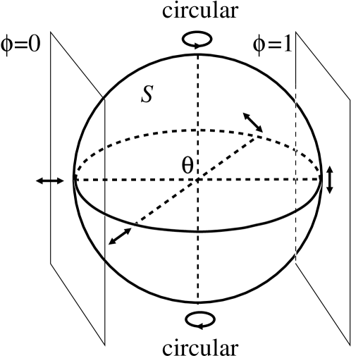
Figure 4: Multiple experiments justify the representation of the photon polarization states in form of the 1-qubit (Bloch) sphere in $\mathbb{R}^{3}$. Once fixed the image, the geometry of $S$ determines uniquely the “transition probabilities” between any pair of pure states. On the figure: the pair of support planes $\phi=1$ and $\phi=0$ illustrates the maximally selective counter which detects all photons in the vertical polarization $\updownarrow$ , but none in the horizontal $\leftrightarrow$. The intermediate values of $\phi$ on the congruence of parallel planes intersecting $S$ define the transition probabilities from all other states to the vertical one $\updownarrow$.

Indeed, $|\langle\psi,\varphi\rangle|^{2}$ not only defines the fraction of the $\varphi$-particles accepted by the $\psi$-filter, but also the fundamental impossibility of accepting less! Every physical process which leads to a certain macroscopic effect for all $\psi$-particles, must lead to the same effect at least for the fraction $|\langle\psi,\varphi\rangle|^{2}$ of $\varphi$-particles. The purely geometric nature of this law, independent of any analytic expression can be best illustrated by the Bloch sphere of the photon polarization states (see Fig. 4) on which the linear polarizations occupy a great circle (the “equator”), circular polarizations are the poles, and the remaining surface points are the elliptic polarizations. The interior of the sphere collects the mixed polarizations, the center $\theta$ representing the complete polarization chaos. The pair of tangent planes $\phi=1$ and $\phi=0$ represents a maximally selective counter detecting all photons in the vertical polarization and rejecting the orthogonal one. The geometry of the sphere $S$ determines immediately the “transition probabilities” between any two pure states without the need of using the analytic $|\varphi\rangle\langle\varphi|$ representation (thus, e.g., the detection ratio between any linear and circular polarization is 1/2).

In case of non-classical ensembles, the geometry of $S$ expresses still more fundamental law about the indistinguishability of quantum mixtures, the phenomenon which appears if $S$ is not a simplex. Given a mixed ensemble of non-classical objects, one cannot, in general, retrospect and find out how the mixture has been prepared. Two mixtures composed of different collections of pure states can be physically indistinguishable (see also Fig. 1).

In the Bloch sphere of polarization states (Fig. 4) the effect is exceptionally simple for its center $\theta$ which can be represented equivalently as a mixture of any pair of orthogonal linear polarizations, or two opposite circular polarizations or in any other way:

$$\begin{split}\theta&\equiv\frac{1}{2}\updownarrow+\frac{1}{2}\leftrightarrow\\ &\equiv\frac{1}{2}\neswarrow+\frac{1}{2}\nwsearrow\\ &\equiv\frac{1}{2}\lcirclearrowleft+\frac{1}{2}\rcirclearrowright\\ &\equiv\cdots\cdots\end{split}$$ (3)

Hence, once having the mixed state $\theta$ one cannot go back and identify its pure components: a kind of statistical paradox making it quite difficult to check experimentally some semantic curiosities of the existing theory, which are still waiting for a good inspiration!

Generalized geometries: are they possible?

The structures reported here contain a certain puzzle. It is basically not strange that the convex geometry is a language of statistical theories. Yet, it was not expected that the structure of an arbitrary convex set $S$ contains the equivalents of principal quantum mechanical concepts. Their properties are distorted, but their meaning is similar. Thus, the logic of properties is an analogue of the quantum logic rf1 and the detection ratios are equivalents of the orthodox “transition probabilities”. In many aspect the Hilbertian schemes are distinguished by their maximal regularity and almost crystalline symmetry: to each face of $S$, (read subspace), corresponds a unique orthocomplement, etc. Might this resemble the relation between the Euclidean and Riemannian geometries? If so then could it happen that in some circumstances the quantum systems could obey the generalized convex geometry, dissenting from the Hilbertian structure?

In the intents of finding a synthesis of the lattice (“logical”) and probabilistic interpretations (since J. von Neumann rf2 ) the statistical aspects, in general, were subordinated to the assumed structure of the orthocomplemented lattice, and the answer of the axiomatic approach was always the same: the quantum mechanics must be exactly as it is. This belief turned even stronger due to the theorem of Gleason rf10 , as well as due to the profound and elegant generalizations of the algebraic approaches of Gel’fand and Naimark rf11 , Haag and Kastler rf12 , Pool rf13 , Araki rf14 , Haag rf15 , and other authors, who never resigned from the Hilbert space representations. Curiously, until today, these convictions find also also a strong support in the well known book of G. Mackey rf16 in which, however, the axiomatic approach has some self-annihilating aspects: after a laborious presentation of six axioms on quantum logic $\mathcal{L}$, the seventh axiom tells flatly that the elements of the logic are closed vector subspaces of a Hilbert space, thus making all previous axioms redundant! (a short report on this school of axiomatics, see H. Primas (rf17, , p. 211)). Some opposition is not so surprising…

The first descriptions of QM based exclusively on the convex geometry belong to G. Ludwig rf18 , though the author adopted axioms in fact limiting the story to the orthodox scheme. The hypothesis about the possibility of quantum mixtures obeying non-Hilbertian geometries was formulated by the present author rf6 ; rf8 , also by Davies and Lewis rf19 . The hypothetical geometries succeeded to awake both positive and hostile reactions. Roger Penrose at some moment hoped that the atypical structures might tell something about the nonlinear graviton rf20 , though later on he complained rf21 that they give a pure statistical interpretation, without any analytical entity behind (though inversely, the nonlinear graviton of Penrose is a pure analytical entity without any statistical interpretation!). T.W. Kibble and S. Randjbar-Daemi followed rf8 describing the classical gravity in interaction with the generalized quantum structure rf22 . Some other authors in philosophy of physics stay firmly on the ground of the orthodox theory. Nonetheless, they don’t escape objections. While Putnam considers the orthocomplemented structure of Hilbert spaces the “truth of quantum mechanics” rf23 (taking the side of Mackey?), John Bell and Bill Hallet rf24 adopt the generalized design proposed in rf6 to show the weakness of Putnam’s argument. However, the deformed geometries, if real, must occur in some concrete physical circumstances. Where should we look for them?

As it seems, the most natural possibility is to look for nonlinear variants of quantum mechanics. In fact, already some simple nonlinear cases of the Schrödinger’s equation admit nonquadratic, positive, absolutely conservative quantities which could be used to define the probability densities rf8 . The quantum mechanics with logarithmic nonlinearity permits to define consistently the reduction of the wave packets rf25 . Yet, as shown by Haag and Bannier rf26 , subsequently also in rf27 , the nonlinear wave equations lead to high mobility of quantum states, breaking the quantum impossibility principles.

The most basic difficulty was noticed by N. Gisin, who had shown that if the linear evolution law of quantum states were amended by adding some nonlinear operations, then the breaking of the mixture indistinguishability would make possible to read the instantaneous messages between parts of the entangled particle systems rf28 ; rf28a . The simplest case would occur in a variant of EPR experiment for the sequences of photon pairs in the singlet polarization state $|\Xi\rangle=\frac{1}{\sqrt{2}}(|\updownarrow\rangle|\leftrightarrow\rangle-|\leftrightarrow\rangle|\updownarrow\rangle)$ emitted in two opposite directions. According to the present day theory the polarization measurements on the left photons can produce at distance (due to the correlation mechanism) any desired mixture (3) of the right photons (or vice versa). As long as mixtures (3) are indistinguishable, this does not transmit information. However, if the observer of the right photon states could cause their nonlinear evolution, he could distinguish the quantum mixtures (3), thus reading hidden information and reconstructing without delay the measurements performed by his distant counterpart on the left EPR photons. So, is the nonlinear QM impossible?

Perhaps, we should not overestimate the axiomatic approaches. What they usually tell is that we cannot modify just one element of the theory, while leaving the whole rest intact. If in the last decade of XIX century some excellent axiomaticians tried to formulate reasonable axioms defining the space-time structure, they would prove beyond any doubt that the space-time must be Galilean! Yet, it is not. The deviations (in our normal conditions) are very small, but rather important…

What can be impossible in QM, is to conserve the orthodox representation of pure states as the “rays” in a complex Hilbert space, together with the tensor product formalism, and with the unitary background evolution, but to extend it by adding some nonlinear evolution operations and to expect that the instantaneous information transfers will be still blocked. However, the whole deduction might be already overloaded by too many axioms. If the evolution were extended by some nonlinear operations, then in the first place, we would loose the Hilbert space orthogonality together with the trace rules for probabilities even without worrying about the superluminal messages…

Returning to the spin or polarization qubits, the possibilities of generalizing the Hilbertian structures depends not so much on axioms but rather on precise knowledge of probabilities. If indeed exactly orthodox, then may be, the qubits can only rigidly rotate…

The problems of systems traditionally described by multi- or infinitely-dimensional Hilbert spaces are more difficult. The questions of Hans Primas, perhaps are still waiting for a good answer: Does quantum mechanics apply to large molecular systems?… Why do so many stationary states not exist? (see (rf18, , p. 11 and 12)). Indeed, even the problem of how to create in practice the one particle states described by arbitrary wave packets deserves systematic studies rf29 ; rf30 ; rf31 ; rf32 .

As recently noticed, the non-linear modifications of quantum dynamics instead of just extending the techniques of the state manipulation might introduce constrains, with the restricted $S$ no longer obeying the Hilbertian geometry rf33 ; an option which might be worth exploring.

All the attempts to see more freedom in quantum structures need some empirical criteria, which would permit to detect the new geometries if they exist. In case of classical state structures such criteria were found by John Bell, in form of Bell inequalities expressing the Boolean geometry of the state mixtures. Their breaking was the sign that the ensembles are non-classical. The problems of quantum ensembles, e.g., whether they indeed obey the Hilbert space geometry, are significantly more involved. The initiative of our colleagues rf9 to describe them in terms of “apophatic” (forbidden) properties continues indeed the effort of John Bell on the new theory level. Some interesting cases might be the “cross sections” of $S$, resembling the “constrained QM” discussed in rf33 , and the projections (the collapsed $S$ caused by deficiency of observables?). Simultaneously, the mathematical research presented in rf7 ; rf9 is an unexpected school of modesty for all of us, who believed to understand so well the property of nice objects called the “density matrices”. Now it turns out that we did not even know the properties of the simple qutrit! Needless to say, should any of the “forbidden properties” be detected for any statistical ensemble in some physical conditions, this will be the proof that the theory is at the new conceptual level. Interesting, what about all that will think the physicists of XXII century?

References

- (1) G. Birkhoff and J. von Neumann, Ann. of Math. 37, 823–843 (1936).
- (2) J. von Neumann, Mathematical Foundations of Quantum Mechanics, Princeton Unv. Press (1955).
- (3) D. Finkelstein, Trans. N.Y. Acad. Sci. 25, 621–637 (1962).
- (4) V.S. Varadarajan, Geometry of Quantum Theory, Van Nostrand, vol 1 (1968), vol 2 (1970).
- (5) C. Piron, Helv. Phys. Acta, 37, 439–468 (1964); Found. Phys. 2, 287–314 (1972).
- (6) B. Mielnik, Commun. Math. Phys. 15, 1–45 (1969).
- (7) I. Bengtsson and K. Życzkowski. GEOMETRY OF QUANTUM STATES, An Introduction to Quantum Entanglement, Cambridge Univ. Press (2006).
- (8) B. Mielnik, Commun. Math. Phys. 37, 221–225 (1974).
- (9) I. Bengtsson, S. Weis and K. Życzkowski, Geometry of the set of mixed quantum states: Apophatic approach, preprint arXiv:1112.2347.
- (10) A.M. Gleason, J. Math. Mech. 6, 885–893 (1957).
- (11) I.M. Gel’fand and M.A. Naimark, Math. Sbornik 12, 197–213 (1943).
- (12) R. Haag and D. Kastler, J. Math. Phys. 5, 848–861 (1964).
- (13) J.C.T. Pool, Commun. Math. Phys. 9, 118 (1968); 9, 212 (1968).
- (14) H. Araki, Pacific J. Math 50, 309–354 (1979.
- (15) R. Haag, Local Quantum Physics, Fields, Particles, Algebras, Springer-Verlag, 2-nd Edition (1996).
- (16) G.W. Mackey, The mathematical foundations of quantum mechanics, Benjamin, New York (1963).
- (17) H. Primas, Chemistry, Quantum Mechanics and Reductionism, Perspectives in Theoretical Chemistry, Springer-Verlag, Berlin-Heidelberg (1983).
- (18) G. Ludwig, Z. Phys. 181, 233–260 (1964).
- (19) E.B. Davies and J.T. Lewis, Commun. Math. Phys. 17, 239–260 (1970).
- (20) R. Penrose, Gen. Rel. Grav. 7, 171–176 (1976).
- (21) The Large, the Small and the Human Mind, Cambridge Univ. Press (1997).
- (22) T.W.B. Kibble and S. Randjbar-Daemi, J. Phys. A 13, 141–148 (1980).
- (23) H. Putnam, The Logic of Quantum Mechanics, Philosophical Papers, vol. 1, Cambridge Univ. Press (1975).
- (24) J. Bell and B. Hallet, Philosophy of Science 49, 355–379 (1982).
- (25) I. Białynicki-Birula and J. Mycielski, Annals of Physics 100, 62 (1976).
- (26) R. Haag and U. Bannier, Commun. Math. Phys. 60, 1–6 (1978).
- (27) B. Mielnik, Commun. Math. Phys. 101, 323–339 (1985).
- (28) N. Gisin, Phys. Lett A 143,1–2 (1989).
- (29) C. Simon, V. Buzek and N. Gisin, Phys. Rev. Lett. 87, 17 (2001).
- (30) D.J. Fernandez and B. Mielnik, J. Math. Phys. 35, 2083 (1994).
- (31) F. Delgado and B. Mielnik, Phys. Lett. A 249, 369 (1998).
- (32) B. Mielnik and O. Rosas-Ortiz, J. Phys. A 37, 10007–10035 (2004).
- (33) B. Mielnik and A. Ramirez, Phys. Sci. 84, 045008 (2011).
- (34) D.C. Brody, A.C.T. Gustavsson and L.P. Hugston, J. Phys. A 43 082003 (2010).