Charge carrier localisation in disordered graphene nanoribbons

Keywords: graphene, local density of states, disorder effects, metal-insulator transition

Abstract. We study the electronic properties of actual-size graphene nanoribbons subjected to substitutional disorder particularly with regard to the experimentally observed metal-insulator transition. Calculating the local, mean and typical density of states, as well as the time-evolution of the particle density we comment on a possible disorder-induced localisation of charge carriers at and close to the Dirac point within a percolation transition scenario.

1 Introduction

Transport in graphene nanoribbons (GNRs) is strongly affected by disorder effects which can be traced back, for example, to dislocations or charged impurities in the substrate, to adatoms adsorbed at the graphene surface, to edge defects, or to ripples associated with the soft structure of graphene. When modelling disorder, many theoretical studies resort to the generic Anderson model [1], which exhibits a disorder-induced localisation transition in three dimensions (3D) that is absent in lower dimensions, however. One-parameter scaling theory predicts that all states are localised for the infinite Anderson-disordered 2D system [2]. The recently observed metal-insulator transition in hydrogenated graphene [3], disordered GNRs [4], and Si-MOSFET inversion layers [5] is beyond reach of the Anderson model, but might be explainable by percolation-based approaches [6, 4].

The classical (geometric) problem of percolation consists in finding a connected path of accessible sites that spans the whole lattice. On the honeycomb lattice, for site-percolation, this will be the case for a concentration of accessible sites $p>p_{c}\approx 0.697$ [7]. For real materials the strict distinction between accessible and blocked sites seems to be too simplistic. For example, upon hydrogenation, the $\pi$-bonds of some carbon atoms within a graphene sheet will be blocked just partly. Also the electron-hole puddles resulting from charged impurities in the substrate lead to a finite difference between the on-site potentials only. Then, tunneling effects between the puddles may become possible, allowing for transport despite the absence of a percolating cluster. In the quantum case, a spanning cluster does not guarantee transport since scattering at its irregular boundaries causes interference effects which may lead to localisation of the charge carriers.

To analyse the localisation properties of low-dimensional systems within numerical approaches, both sophisticated algorithms and highly efficient implementations are mandatory since the relevant length scales are exceptionally large. In this regard the finite extension of mesoscopic graphene flakes or GNRs deserves further attention since it may mask localisation effects if the localisation length exceeds the system size.

In this work we investigate the electronic properties of GNR eigenstates in the vicinity of the Dirac point using a local distribution approach based on exact diagonalisation (ED) techniques [8]. This method has proven its reliability for the study of Anderson localisation and quantum percolation on various lattices in different dimensions. [9, 10]

2 Model and method

To model disordered GNRs we consider the tight-binding Hamiltonian

$${H}=-\bar{t}\sum\limits_{\langle ij\rangle}\bigl{(}{c}_{i}^{{\dagger}}{c}_{j}+\text{H.c.}\bigr{)}+\sum\limits_{j=1}^{N}\epsilon_{j}{c}_{j}^{{\dagger}}{c}_{j}$$ (1)

on a honeycomb lattice with $N$ sites, including electron transfer $\bar{t}$ between nearest neighbours $\langle ij\rangle$ only. In Eq. (1), $c_{i}^{{\dagger}}$ $(c_{i})$ creates (annihilates) an electron at lattice site $i$. Drawing the on-site potentials $\epsilon_{i}$ from the bimodal distribution

$$p[\epsilon_{j}]=p\,\delta(\epsilon_{j}-\epsilon_{A})+(1-p)\,\delta(\epsilon_{j}-\epsilon_{B})\;,$$ (2)

sites are occupied by an atom of type $A$ [$B$] with probability $p$ [$(1-p)$] (binary alloy analogy). Without loss of generality we choose the on-site energy of the majority sub-band $\epsilon_{A}=0$, use $\Delta=\epsilon_{B}-\epsilon_{A}$ hereafter, and let $\bar{t}$ fix the unit of energy.

Localisation properties of disordered systems can be discussed in terms of the local density of states (LDOS),

$$\rho_{i}(E)=\sum\limits_{n=1}^{N}|\langle i|n\rangle|^{2}\,\delta(E-E_{n})\;,$$ (3)

where $|i\rangle=c^{{\dagger}}_{i}|0\rangle$, and $|n\rangle$ is a single-electron eigenstate of $H$ with energy $E_{n}$. The LDOS can be determined very efficiently by the Kernel Polynomial Method which is an expansion of the rescaled Hamiltonian into a finite series of Chebyshev polynomials [11]. Thereby an energy level broadening appears that can be controlled by the expansion order.

Within the local distribution approach one has to analyse the behaviour of the normalised LDOS distribution $f[\rho_{i}/\rho_{\text{me}}]$ upon finite-size scaling for many realisations of disorder (here $\rho_{\text{me}}=\langle\rho_{i}\rangle$ is the mean DOS). While extended states are characterised by a system-size independent $f[\rho_{i}/\rho_{\text{me}}]$, the distribution for localised states strongly depends on $N$; its maximum shifts towards zero and finally $f[\rho_{i}/\rho_{\text{me}}]$ becomes singular as $N\to\infty$. Since in many cases $f[\rho_{i}/\rho_{\text{me}}]$ closely resembles a log-normal distribution [10], a simplified discussion may use the typical DOS, $\rho_{\text{ty}}=e^{\langle\ln(\rho_{i})\rangle}$, which is directly related to the maximum of the log-normal distribution.

Alternatively we may access the localisation properties of a system by determining the recurrence probability $P_{R}(t\to\infty)$, which in the thermodynamic limit is finite for localised states and scales to zero as $1/N$ for extended states. Again a finite series expansion into Chebyshev polynomials is promising, in this case applied to the time evolution operator [9]. Then, for example, we may track how an initially localised wave packet evolves in time by calculating the time dependent local particle density,

$$|\psi({\mathbf{r}}_{i},t)|^{2}=\Big{|}\sum\limits_{m=1}^{N}e^{-{\mathrm{i}}E_{m}t}\langle m|\psi(0)\rangle\langle i|m\rangle\Big{|}^{2}\;.$$ (4)

3 Numerical results

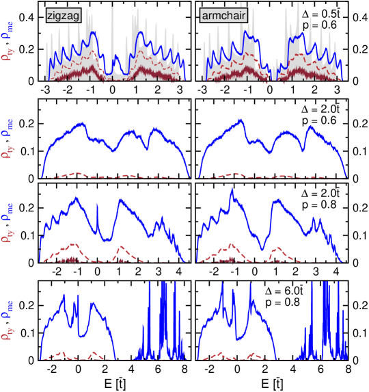
Figure 1: Mean (solid blue) and typical (dashed red) DOS for zigzag (left column, $N_{z}=6$) and armchair (right column, $N_{a}=10$) GNRs of width $W=1.1\,\mathrm{nm}$ and periodic boundary conditions in longitudinal direction. In each panel $\rho_{\text{ty}}$ is given for $L=213\,(1064)\,\mathrm{nm}$ by red dashed (dark-red long-dashed) lines for $6\times 10^{4}$ realisations of disorder. These system sizes correspond to $10000$ $(50000)$ lattice sites for the armchair and $10392$ $(51960)$ for the zigzag case. For comparison the mean DOS for pristine GNRs is given in grey in the top panels.

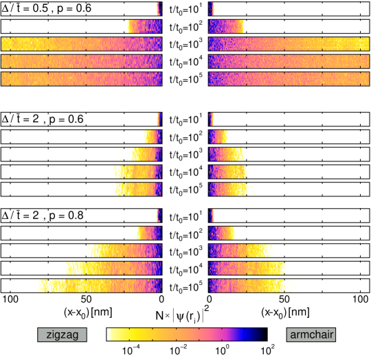
Figure 2: Time evolution of the normalised particle density $N|\psi({\mathbf{r}}_{i})|^{2}$ for disordered GNRs. Device dimensions (only one half is shown): $(1.1\times 213)\,\text{nm}^{2}$ corresponding to $6\times 1732$ atoms (zigzag) and $10\times 1000$ atoms (armchair). Times are measured in units of the inverse hopping element $t_{0}=1/\bar{t}$.

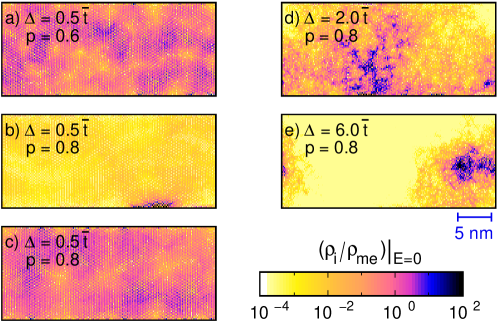
Figure 3: Normalised LDOS $(\rho_{i}/\rho_{\text{me}})|_{E=0}$ for particular zigzag GNRs with $256\times 64$ sites as obtained by exact diagonalisation. In contrast to the other panels, where the LDOS is calculated at the unperturbed Dirac point, $E=0$, panel (c) refers to $E^{-}=-0.007\bar{t}$.

As compared to mesoscopic graphene flakes, the DOS of ordered GNRs exhibits a series of spikes (van Hove singularities) indicating quasi-1D behaviour. The number and position of these spikes depend on the ribbon geometry and on the (finite) number of unit cells in the transverse cross section. Furthermore, GNRs form very interesting edge states. While for armchair edges there is a gap at the Dirac point, $E=0$, a variety of degenerate edge states exist for zigzag edges (see top panel of Fig. 1).

Accounting for adatoms that lead to random on-site potentials $\Delta$, a “copy” of the DOS centred around $\Delta$ will appear. The random superposition of the local A- and B-atom DOS results in the total (mean) DOS presented in Fig. 1. Increasing the value of $\Delta$ enhances the random on-site fluctuations, and at $\Delta=6\bar{t}$ (bottom panel of Fig. 1) we enter a split-band regime, where two distinct sub-bands emerge.

The decay of $\rho_{\text{ty}}$ with increasing system size indicates that the states are localised in principle for any of the shown parameters; actually $\rho_{\text{ty}}$ vanishes for $N\sim 5\times 10^{4}$ already in all panels except for those in the top most row. There, however, the finite value of $\rho_{\text{ty}}$ solely indicates that the localisation length is larger than the system size or comparable to it.

Figure 2 shows the time evolution of an initially localised state, as calculated by the Chebyshev method. After an initial, fast spreading process ($t\lesssim 10^{4}t_{0}$) the wave function becomes quasi-stationary, i.e., there are temporal amplitude fluctuations on individual sites but the overall region of sites having finite amplitudes remains constant. Moderate ribbon lengths and small values of $\Delta$ result in a localisation length larger than the system size (top panel of Fig. 2) and therefore cause a “metallic” behaviour of the GNR. In contrast, for larger $\Delta$ the wave packet remains localised even for rather small systems. Clearly the wave function stays more localised for $p=0.6<p_{c}$ than for $p=0.8>p_{c}$, since due to the lack of a spanning cluster in the first case, the spreading of the wave function depends heavily on quantum tunneling, whose efficiency decreases as $\Delta$ increases.

To illustrate the localisation properties of our binary-alloy GNR model in more detail, we present ED results for the normalised LDOS in Fig. 3, focusing thereby on energies close to the (unperturbed) Dirac point, $E=0$. Although for a small potential difference $\Delta$ and a nearly equal concentration of A and B atoms the wave function spans the entire (finite) lattice, the bimodal distribution still shows up by two interpenetrating regions with large and small wave-function amplitudes [see Fig. 3 (a)]. A stronger asymmetry in the concentration of type A and B atoms then leads to a localisation of the wave function in small regions near the GNR’s edge [cf. Fig. 3 (b)]. As may be expected the wave-function localisation effect becomes more pronounced at larger $\Delta$, i.e. the localisation length clearly decreases upon increasing $\Delta$ [see Fig. 3 (d) and (e)]. Note, however, that for $p=0.8$ a spanning cluster exists, that is we observe a true quantum percolation effect.

A particularly interesting feature is the complete change in character of the eigenstates when crossing the energy of the unperturbed Dirac point for slightly differing on-site potentials and asymmetric distribution of the atom variants. While for $E=0^{+}$ [Fig. 3 (b)], the state is clearly localised, states on the opposite side of the impurity sub-band, $E=0^{-}$, are extended [Fig. 3 (c)]. This transition is absent for a less pronounced asymmetry between the two atom types, e.g. for $p=0.6$ in [Fig. 3 (a)].

In conclusion, we have argued theoretically and demonstrated numerically by zero-tempera-ture exact diagonalisation calculations that disorder of binary-alloy type in combination with quantum percolation effects will strongly affect electron transport in graphene nanoribbons, up to the point of a disorder-induced localisation of the charge carriers. We argue that in order to corroborate such kind of quantum localisation, transport measurements should be performed at much lower temperatures than used so far, but even so the effect might be covered by the large localisation lengths compared to the spatial dimensions of actual GNRs.

References

- [1] P. W. Anderson. Phys. Rev., 109:1492, 1958.
- [2] E. Abrahams, P. W. Anderson, D. C. Licciardello, and T. V. Ramakrishnan. Phys. Rev. Lett., 42:673, 1979.
- [3] A. Bostwick, J. L. McChesney, K. V. Emtsev, T. Seyller, K. Horn, S. D. Kevan, and E. Rothenberg. Phys. Rev. Lett., 103:056404, 2009.
- [4] S. Adam, S. Cho, M. S. Fuhrer, and S. Das Sarma. Phys. Rev. Lett., 101:046404, 2008.
- [5] S. V. Kravchenko, G. V. Kravchenko, J. E. Furneaux, V. M. Pudalov, and M. D’Iorio. Phys. Rev. B, 50:8039, 1994; S. V. Kravchenko, W. E. Mason, G. E. Bowker, J. E. Furneaux, V. M. Pudalov, and M. D’Iorio. Phys. Rev. B, 51:7038, 1995.
- [6] S. Das Sarma, M. P. Lilly, E. H. Hwang, L. N. Pfeiffer, K. W. West, and J. L. Reno. Phys. Rev. Lett., 94:136401, 2005.
- [7] P. N. Suding and R. M. Ziff. Phys. Rev. E, 60:275, 1999.
- [8] A. Alvermann and H. Fehske. Lect. Notes Phys., 739:505, 1999.
- [9] G. Schubert and H. Fehske. Phys. Rev. B, 77:245130, 2008; G. Schubert, J. Schleede and H. Fehske. Phys. Rev. B, 79:235116, 2009.
- [10] G. Schubert, J. Schleede, K. Byczuk, H. Fehske, and D. Vollhardt. Phys. Rev. B, 81:155106, 2010.
- [11] A. Weiße, G. Wellein, A. Alvermann, and H. Fehske. Rev. Mod. Phys., 78:275–306, 2006.