Performance Analysis of $\ell_{1}$-synthesis with Coherent Frames

Abstract

Signals with sparse frame representations comprise a much more realistic model of nature than that with orthonomal bases. Studies about the signal recovery associated with such sparsity models have been one of major focuses in compressed sensing. In such settings, one important and widely used signal recovery approach is known as $\ell_{1}$-synthesis (or Basis Pursuit). We present in this article a more effective performance analysis (than what are available) of this approach in which the dictionary ${\bf D}$ may be highly, and even perfectly correlated. Under suitable conditions on the sensing matrix ${\bf\Phi}$, an error bound of the recovered signal $\hat{{\bf f}}$ (by the $\ell_{1}$-synthesis method) is established. Such an error bound is governed by the decaying property of $\tilde{{\bf D}}_{\text{o}}^{*}{\bf f}$, where ${\bf f}$ is the true signal and $\tilde{{\bf D}}_{\text{o}}$ denotes the optimal dual frame of ${\bf D}$ in the sense that $\|\tilde{{\bf D}}_{\text{o}}^{*}\hat{{\bf f}}\|_{1}$ produces the smallest $\|\tilde{{\bf D}}^{*}\tilde{{\bf f}}\|_{1}$ in value among all dual frames $\tilde{{\bf D}}$ of ${\bf D}$ and all feasible signals $\tilde{{\bf f}}$. This new performance analysis departs from the usual description of the combo $\mbox{${\bf\Phi}$}{\bf D}$, and places the description on ${\bf\Phi}$. Examples are demonstrated to show that when the usual analysis fails to explain the working performance of the synthesis approach, the newly established results do.

Keywords: Compressed sensing, coherent frames, $\ell_{1}$-synthesis, optimal-dual-based $\ell_{1}$-analysis.

1 Introduction

Compressed sensing is a new data acquisition theory which allows that sparse or compressible signals of interest can be recovered from a small number of linear, non-adaptive, and usually randomized measurements [8, 9, 13]. By now, compressed sensing has attacked abundant applications in signal and image processing, see e.g., the two special issues [1], [2] and references therein. Formally, one considers the following measurement model:

$${\bf y}=\mbox{${\bf\Phi}$}{\bf f}+{\bf z},$$ (1)

where ${\bf\Phi}$ is an $m\times n$ sensing matrix with $m\ll n$ (indicating some significant undersampling) and ${\bf z}\in{\mathbb{R}}^{m}$ is a noise term modeling measurement error. The goal is to reconstruct the unknown signal ${\bf f}\in{\mathbb{R}}^{n}$ based on available measurements ${\bf y}\in{\mathbb{R}}^{m}$.

In standard compressed sensing scenarios, it is usually assumed that the signal ${\bf f}$ has a sparse (or nearly sparse) representation in an orthonormal basis. However, a large number of applications in signal and image processing point to problems where ${\bf f}$ is sparse with respect to an overcomplete dictionary or a frame rather than an orthonormal basis, see, e.g., [24], [11], [4], and references therein. Examples include, e.g., signal modeling in array signal processing (oversampled array steering matrix), reflected radar and sonar signals (Gabor frames), and images with curves (curvelets), etc. The flexibility of frames is the key characteristic that empowers frames to become a natural and concise signal representation tool. Therefore, it is highly desirable to extend the compressed sensing methodology to redundant dictionaries as apposed to orthnormal bases only, see, e.g., [25], [10], [22]. In such sparse frame representation setting, the signal ${\bf f}$ is now expressed as ${\bf f}={\bf D}{\bf x}$ where ${\bf D}\in{\mathbb{R}}^{n\times d}$ ($n<d$) is a matrix of frame vectors (as columns) that are often rather coherent in applications, and ${\bf x}\in{\mathbb{R}}^{d}$ is a sparse coefficient vector. The linear measurements of ${\bf f}$ then can be written as

$${\bf y}=\mbox{${\bf\Phi}$}{\bf D}{\bf x}+{\bf z}.$$ (2)

Since ${\bf x}$ is assumed sparse, the standard way of recovering ${\bf f}$ from (2) is known as $\ell_{1}$-synthesis (or synthesis-based method) [11], [16], [10]. From the measurements, one first finds the sparsest possible coefficient ${\bf x}$ by solving an $\ell_{1}$ minimization problem

$$\hat{{\bf x}}=\underset{\tilde{{\bf x}}\in{\mathbb{R}}^{d}}{\textrm{argmin}}\|\tilde{{\bf x}}\|_{1}\ \ \ \ s.t.\ \ \|{\bf y}-\mbox{${\bf\Phi}$}{\bf D}\tilde{{\bf x}}\|_{2}\leq\epsilon,$$ (3)

where $\|{\bf x}\|_{p}\ (p=1,2)$ denotes the standard $\ell_{p}$-norm of the vector ${\bf x}$ and $\epsilon$ is an upper bound of the noise. Then the solution to ${\bf f}$ is derived via a synthesis operation, i.e., $\hat{{\bf f}}={\bf D}\hat{{\bf x}}$.

Although empirical studies show that $\ell_{1}$-synthesis often achieves good recovery results, the theoretical performance of this method is far from satisfactory. The analytical results in [25] essentially require that the frame ${\bf D}$ has columns that are extremely uncorrelated such that the compound matrix $\mbox{${\bf\Phi}$}{\bf D}$ satisfies the requirements imposed by the traditional compressed sensing assumptions. However, these requirements are often infeasible when ${\bf D}$ is highly coherent. For example, consider a simple case in which $\mbox{${\bf\Phi}$}\in{\mathbb{R}}^{m\times n}$ is a Gaussian matrix with i.i.d. entries, then $\mbox{${\bf\Phi}$}\sim{\cal N}\,({\bf 0},{\bf I}_{n}\otimes{\bf I}_{m})$, where $\otimes$ denotes the Kronecker product and ${\bf I}_{m}$ is an identity matrix of the size $m$. It is now well known that with very high probability ${\bf\Phi}$ satisfies the restricted isometry property (RIP) [6] provided that $m$ is on the order of $s\log(n/s)$ [3], [8]. Let us now examine $\mbox{${\bf\Phi}$}{\bf D}$. It is not hard to show that $\mbox{${\bf\Phi}$}{\bf D}\sim{\cal N}\,({\bf 0},{\bf D}^{*}{\bf D}\otimes{\bf I}_{m})$, where $(\cdot)^{*}$ denotes the transpose operation. If ${\bf D}$ is unitary, then $\mbox{${\bf\Phi}$}{\bf D}$ has the same distribution as ${\bf\Phi}$, and hence satisfies the RIP. However, if ${\bf D}$ is a coherent frame, then $\mbox{${\bf\Phi}$}{\bf D}$ may no longer obey the common RIP since the entries of $\mbox{${\bf\Phi}$}{\bf D}$ are correlated. Meantime, the mutual incoherence property (MIP) [14] may not apply either, as it is very hard for $\mbox{${\bf\Phi}$}{\bf D}$ to satisfy the MIP as well when ${\bf D}$ is highly correlated.

The perspective of the results in [25] is that some sufficient conditions are put on the compound matrix $\mbox{${\bf\Phi}$}{\bf D}$ such that ${\bf x}$ can be recovered accurately, which leads to a good estimate of ${\bf f}$. However, if one is only interested in reconstructing the signal ${\bf f}$ and may not care about obtaining a good recovery of ${\bf x}$. As pointed out in [10], when the dictionary ${\bf D}$ has two identical columns, it seems impossible to recover a unique sparse coefficient vector ${\bf x}$ from the measurements, but we may certainly be able to reconstruct the signal ${\bf f}$ accurately. In other words, a good recovery of ${\bf x}$ may be unnecessary to guarantee an accurate reconstruction of ${\bf f}$.

We observe in abundant examples that the $\ell_{1}$-synthesis method is also capable of producing fine approximation of ${\bf f}$ without recovering accurate coefficient vector ${\bf x}$. Known analysis results such as [25] would then not be able to explain these fine results by the synthesis approach.

In this article, we present a new performance analysis for the $\ell_{1}$-synthesis approach (3) in which the dictionary ${\bf D}$ may be highly - and even perfectly - correlated. To the best knowledge of the authors, our new results are more effective than what are known and available. Our results do not depend on a good recovery of the coefficients. The basic idea is to establish the equivalence between the $\ell_{1}$-synthesis approach and the optimal-dual-based $\ell_{1}$-analysis approach recently proposed in [22]. Then the recovery error bound for the latter will naturally lead to that for the former.

This paper is organized as follows. Section 2 introduces the family of analysis-based approaches which includes the standard $\ell_{1}$-analysis, the general-dual-based $\ell_{1}$-analysis, and the optimal-dual-based $\ell_{1}$-analysis. In Section 3, the equivalence between the $\ell_{1}$-synthesis and the optimal-dual-based $\ell_{1}$-analysis is established. The new performance analysis (error bound) for the $\ell_{1}$-synthesis is then naturally followed from that of the optimal-dual based $\ell_{1}$-analysis approach. Some numerical experiments are presented in Section 4 to demonstrate the effectiveness of the results obtained in Section 3. These examples show that when the usual analysis fails to explain the working performance of the synthesis approach, our newly established results do. Conclusion remarks are given in Section 5.

2 The Family of Analysis-based Approaches Based on General Dual Frames

Alongside the $\ell_{1}$-synthesis approach, there is a counterpart that takes an analysis point of view, see e.g., [15], [16], [10]. This alternative finds an estimate of ${\bf f}$ directly by solving the problem

$$\hat{{\bf f}}=\underset{\tilde{{\bf f}}\in{\mathbb{R}}^{n}}{\textrm{argmin}}\|\bar{{\bf D}}^{*}\tilde{{\bf f}}\|_{1}\ \ \ \ s.t.\ \ \|{\bf y}-\mbox{${\bf\Phi}$}\tilde{{\bf f}}\|_{2}\leq\epsilon,$$ (4)

where $\bar{{\bf D}}$ denotes the canonical dual frame of ${\bf D}$, i.e., $\bar{{\bf D}}=({\bf D}{\bf D}^{*})^{-1}{\bf D}$. Note that if ${\bf D}$ is a Parseval frame, then we have $\bar{{\bf D}}={\bf D}$.

It is well known by now [16] that when ${\bf D}$ is a square and invertible dictionary, the $\ell_{1}$-analysis and $\ell_{1}$-synthesis approaches are equivalent. However, when ${\bf D}$ is an overcomplete frame, the gap between them exists.

A remarkable performance study of the $\ell_{1}$-analysis approach (4) in the case of Parseval frames ($\bar{{\bf D}}={\bf D}$) was given in [10]. It was shown that, under suitable conditions on the sensing matrix ${\bf\Phi}$, the solution to (4) is very accurate provided that ${\bf D}^{*}{\bf f}$ has rapidly decreasing coefficients. In other words, when the frame coefficient vector ${\bf D}^{*}{\bf f}$ is reasonably sparse, $\ell_{1}$-analysis can be the right method to use.

However, that ${\bf f}$ is sparse in terms of ${\bf D}$ does not imply ${\bf D}^{*}{\bf f}$ is necessarily sparse. In fact, as the canonical dual frame expansion in the case of Parseval frames, ${\bf D}^{*}{\bf f}={\bf D}^{*}{\bf D}{\bf x}$ has the minimum $\ell_{2}$-norm by the frame property, see, e.g., [12] and is usually fully populated which is also pointed out in [25]. In other words, the canonical dual frame of ${\bf D}$ may be ineffective in sparsifying ${\bf f}$ since $\ell_{2}$-norm tends to spread the coefficients into a large number of small coefficients.

To overcome this difficulty, the standard $\ell_{1}$-analysis approach (4) has recently been extended to a more general case in which the analysis operator can be any dual frame of ${\bf D}$ [22]. This leads to the following general-dual-based $\ell_{1}$-analysis approach

$$\hat{{\bf f}}=\underset{\ \tilde{{\bf f}}\in{\mathbb{R}}^{n}}{\textrm{argmin}}\|\tilde{{\bf D}}^{*}\tilde{{\bf f}}\|_{1}\ \ \ \ s.t.\ \ \|{\bf y}-\mbox{${\bf\Phi}$}\tilde{{\bf f}}\|_{2}\leq\epsilon,$$ (5)

where columns of $\tilde{{\bf D}}$ form a general (and any) dual frame of ${\bf D}$. The performance analysis of the general-dual-based $\ell_{1}$-analysis approach was also given in [22]. In order to introduce the results, we require the concept of ${\bf D}$-RIP [10]: An $m\times n$ sensing matrix ${\bf\Phi}$ is said to satisfy the restricted isometry property adapted to ${\bf D}$ (abbreviated ${\bf D}$-RIP) with constant $\delta_{s}\in(0,1)$ if

$$(1-\delta_{s})\|{\bf v}\|_{2}^{2}\leq\|\mbox{${\bf\Phi}$}{\bf v}\|_{2}^{2}\leq(1+\delta_{s})\|{\bf v}\|_{2}^{2}$$ (6)

holds for all ${\bf v}\in\Sigma_{s}$, where $\Sigma_{s}$ is the union of all subspaces spanned by all subsets of $s$ columns of ${\bf D}$. The validity of the ${\bf D}$-RIP was discussed in e.g., [10], [20]. It was shown in [10] that any $m\times n$ matrix ${\bf\Phi}$ obeying for any fixed $\mbox{\boldmath$\nu$\unboldmath}\in{\mathbb{R}}^{n}$

$$\mathop{\rm Pr}\left(\left|\|\mbox{${\bf\Phi}$}\mbox{\boldmath$\nu$\unboldmath}\|_{2}^{2}-\|\mbox{\boldmath$\nu$\unboldmath}\|_{2}^{2}\right|\geq\delta\|\mbox{\boldmath$\nu$\unboldmath}\|_{2}^{2}\right)\leq ce^{-\gamma\delta^{2}m},\ \ \ \ \delta\in(0,1)$$ (7)

($\gamma$, $c$ are positive constants) will satisfy the ${\bf D}$-RIP with overwhelming probability provided that $m$ is on the order of $s\log(d/s)$. Many types of random matrices satisfy (7), some examples include matrices with Gaussian, subgaussian, or Bernoulli entries. It has also been shown in [20] that randomizing the column signs of any matrix that satisfies the standard RIP results in a matrix which satisfies the Johnson-Lindenstrauss lemma [19]. Such a matrix would then satisfy the ${\bf D}$-RIP via (7). Consequently, partial Fourier matrix (or partial circulant matrix) with randomized column signs will satisfy the ${\bf D}$-RIP since these matrices are known to satisfy the RIP.

With these preliminaries, we now restate the results in [22] as follows.

Theorem 1.

[22] Let ${\bf D}$ be a general frame of ${\mathbb{R}}^{n}$ with frame bounds $0<A\leq B<\infty$. Let $\tilde{{\bf D}}$ be an alternative dual frame of ${\bf D}$ with frame bounds $0<\tilde{A}\leq\tilde{B}<\infty$, and let $\rho=s/b$. Suppose

$$\left(1-\sqrt{\rho B\tilde{B}}\right)^{2}\cdot\delta_{s+a}+\rho B\tilde{B}\cdot\delta_{b}<1-2\sqrt{\rho B\tilde{B}}$$ (8)

holds for some positive integers $a$ and $b$ satisfying $0<b-a\leq 3a$. Then the solution $\hat{{\bf f}}$ to (5) satisfies

$$\|\hat{{\bf f}}-{\bf f}\|_{2}\leq C_{0}\cdot\epsilon+C_{1}\cdot\frac{\|\tilde{{\bf D}}^{*}{\bf f}-(\tilde{{\bf D}}^{*}{\bf f})_{s}\|_{1}}{\sqrt{s}},$$ (9)

where $C_{0}$ and $C_{1}$ are some constants and $(\tilde{{\bf D}}^{*}{\bf f})_{s}$ denotes the vector consisting the largest $s$ entries of $\tilde{{\bf D}}^{*}{\bf f}$ in magnitude (and setting the other to zero).

Theorem 1 shows that if ${\bf\Phi}$ satisfies some proper conditions, e.g., (8), then the solution to (5) is very accurate provided that $\tilde{{\bf D}}^{*}{\bf f}$ has rapidly decreasing coefficients. By the definition of the ${\bf D}$-RIP, the condition (8) is independent of the coherence of the dictionary ${\bf D}$. For differently chosen $a$ and $b$, (8) will give rise to different conditions on the ${\bf D}$-RIP constants $\delta_{s+a}$ and $\delta_{b}$. For instance, if ${\bf D}$ is a Parseval frame and $\tilde{{\bf D}}$ is its canonical dual frame, i.e., $B\tilde{B}=1$, then (8) is satisfied whenever $\delta_{2s}<0.1398$ [22].

With the error bound (9), we can easily see the potential superiority of using alternative dual frames as analysis operators. For clarity, we consider a simple case in which the noise is free, i.e., $\epsilon=0$. Then the error bound (9) reduces to

$$\|\hat{{\bf f}}-{\bf f}\|_{2}\leq C_{1}\cdot\frac{\|\tilde{{\bf D}}^{*}{\bf f}-(\tilde{{\bf D}}^{*}{\bf f})_{s}\|_{1}}{\sqrt{s}}.$$ (10)

Clearly, the quality of the bound ${\|\tilde{{\bf D}}^{*}{\bf f}-(\tilde{{\bf D}}^{*}{\bf f})_{s}\|_{1}}/{\sqrt{s}}$ in (10) is measured in terms of how effective $\tilde{{\bf D}}^{*}{\bf f}$ is in spasifying the signal ${\bf f}$ with respect to the dictionary ${\bf D}$. To explain, suppose that ${\bf f}$ has a sparse representation in ${\bf D}$, i.e., ${\bf f}={\bf D}{\bf x}$, where ${\bf x}$ is a sparse coefficient vector. As discussed before, the canonical dual frame expansion of ${\bf f}$ has the minimum $\ell_{2}$-norm, i.e., $\|\bar{{\bf D}}^{*}{\bf f}\|_{2}=\underset{\tilde{{\bf x}}:{\bf D}\tilde{{\bf x}}={\bf f}}{\textrm{min}}\|\tilde{{\bf x}}\|_{2}$, and is ineffective in promoting sparsity in general. On the other hand, when the analysis operator can be any dual frame of ${\bf D}$, it is not hard to imagine that there should be some dual frame of ${\bf D}$, denoted by $\tilde{{\bf D}}_{\mathcal{S}}$, such that $\tilde{{\bf D}}_{\mathcal{S}}^{*}{\bf f}={\bf x}$. This is due to the fact that all coefficients of a frame expansion of ${\bf f}$ in ${\bf D}$ should correspond to some dual frame of ${\bf D}$, which really is the spirit of frame expansions. Generally, $\tilde{{\bf D}}_{\mathcal{S}}$ is much more effective in sparsifying the signal ${\bf f}$ than the canonical dual frame does. Therefore, one may expect a better recovery performance by taking some “proper” alternative dual frame as the analysis operator.

The important question then is how to choose some appropriate dual frame such that the corresponding analysis coefficients are as sparse as possible. Since the true ${\bf f}$ is never known before hand in practice, it seems to impossible to explicitly construct some proper dual frame $\tilde{{\bf D}}$ such that $\tilde{{\bf D}}^{*}{\bf f}$ is sparse without additional priori knowledge about the signal ${\bf f}$. One approach proposed in [22] is by the method of optimal-dual-based $\ell_{1}$-analysis:

$$\hat{{\bf f}}=\underset{{\bf D}\tilde{{\bf D}}^{*}={\bf I},\ \tilde{{\bf f}}\in{\mathbb{R}}^{n}}{\textrm{argmin}}\|\tilde{{\bf D}}^{*}\tilde{{\bf f}}\|_{1}\ \ \ \ s.t.\ \ \|{\bf y}-\mbox{${\bf\Phi}$}\tilde{{\bf f}}\|_{2}\leq\epsilon,$$ (11)

where the optimization is performed simultaneously over both all dual frames $\tilde{{\bf D}}$ of ${\bf D}$ and the feasible signal set. This seemingly complicated optimization problem can be reformulated into a simplified form. Note that the class of all dual frames for ${\bf D}$ is given by [21]

$$\tilde{{\bf D}}=({\bf D}{\bf D}^{*})^{-1}{\bf D}+{\bf W}^{*}({\bf I}_{d}-{\bf D}^{*}({\bf D}{\bf D}^{*})^{-1}{\bf D})=\bar{{\bf D}}+{\bf W}^{*}{\bf P},$$ (12)

where ${\bf P}\equiv{\bf I}_{d}-{\bf D}^{*}({\bf D}{\bf D}^{*})^{-1}{\bf D}$ denotes the orthogonal projection onto the null space of ${\bf D}$ and ${\bf W}\in{\mathbb{R}}^{d\times n}$ is an arbitrary matrix. Plug (12) into (11), we obtain

$$(\hat{{\bf f}},\ \hat{{\bf g}})=\underset{\tilde{{\bf f}}\in{\mathbb{R}}^{n},\ {\bf g}\in{\mathbb{R}}^{d}}{\textrm{argmin}}\|\bar{{\bf D}}^{*}\tilde{{\bf f}}+{\bf P}{\bf g}\|_{1}\ \ \ \ s.t.\ \ \|{\bf y}-\mbox{${\bf\Phi}$}\tilde{{\bf f}}\|_{2}\leq\epsilon,$$ (13)

where we have used the fact that when $\tilde{{\bf f}}\neq{\bf 0}$, ${\bf g}\equiv{\bf W}\tilde{{\bf f}}$ can be any vector in ${\mathbb{R}}^{d}$ due to the fact that ${\bf W}$ is free. Note that if ${\bf P}{\bf g}\equiv{\bf 0}$, then (13) reduces to the standard $\ell_{1}$-analysis approach (4). In [22], an iterative algorithm based on the split Bregman iteration [17] was developed to solve the optimization problem (13) efficiently.

Clearly, the solution to (11) definitely corresponds to that of (5) with some “optimal” dual frame, say $\tilde{{\bf D}}_{\text{o}}$ as the analysis operator. The optimality here is in the sense that $\|\tilde{{\bf D}}_{\text{o}}^{*}\hat{{\bf f}}\|_{1}$ achieves the smallest $\|\tilde{{\bf D}}^{*}\tilde{{\bf f}}\|_{1}$ in value among all dual frames $\tilde{{\bf D}}$ of ${\bf D}$ and feasible signals $\tilde{{\bf f}}$ satisfied the constraint in (11). Once $\hat{{\bf f}}$ and $\hat{{\bf g}}$ are obtained (through solving (13)), it follows from (12) that the analysis operator $\tilde{{\bf D}}_{\text{o}}^{*}$ is given by

$$\tilde{{\bf D}}_{\text{o}}^{*}=\bar{{\bf D}}^{*}+{\bf P}{\bf W}_{\text{o}},$$ (14)

with ${\bf W}_{\text{o}}$ satisfying

$$\hat{{\bf g}}={\bf W}_{\text{o}}\hat{{\bf f}}.$$ (15)

Evidently, the optimal dual frame $\tilde{{\bf D}}_{\text{o}}$ depends on the solutions of (13). By utilizing the fact that $\text{vec}({\bf A}{\bf B}{\bf C})=({\bf C}^{*}\otimes{\bf A})\text{vec}({\bf B})$, the above equation (15) is equivalent to

$$(\hat{{\bf f}}^{*}\otimes{\bf I}_{d})\cdot\text{vec}({\bf W}_{\text{o}})=\hat{{\bf g}},$$ (16)

where $\text{vec}({\bf W}_{\text{o}})$ denotes the vectorization of the matrix ${\bf W}_{\text{o}}$ by stacking the columns of ${\bf W}_{\text{o}}$ into a single vector. Evidently, the solution to (16) is non-unique in general since this equation is highly underdetermined with $n$ equations but $nd$ unknowns. The class of solutions to (16) is given by

$$\text{vec}({\bf W}_{\text{o}}) =(\hat{{\bf f}}^{*}\otimes{\bf I}_{d})^{\dagger}\hat{{\bf g}}+\left({\bf I}_{nd}-(\hat{{\bf f}}^{*}\otimes{\bf I}_{d})^{\dagger}(\hat{{\bf f}}^{*}\otimes{\bf I}_{d})\right){\bf w}$$

$$=(\hat{{\bf f}}\otimes{\bf I}_{d})\hat{{\bf g}}/\|\hat{{\bf f}}\|_{2}^{2}+\left({\bf I}_{nd}-(\hat{{\bf f}}\hat{{\bf f}}^{*}\otimes{\bf I}_{d})\right){\bf w}/\|\hat{{\bf f}}\|_{2}^{2},$$ (17)

where ${\bf A}^{\dagger}$ denotes the pseudo-inverse of ${\bf A}$ and ${\bf w}\in{\mathbb{R}}^{nd\times 1}$ is an arbitrary vector. In deriving (2), we have used the two facts that $({\bf A}\otimes{\bf B})^{\dagger}={\bf A}^{\dagger}\otimes{\bf B}^{\dagger}$ and $({\bf A}\otimes{\bf B})({\bf C}\otimes{\bf D})={\bf A}{\bf C}\otimes{\bf B}{\bf D}$, see e.g., [23]. Let ${\bf w}={\bf 0}$, then (2) reduces to the least square solution of ${\bf W}_{\text{o}}$

$${\bf W}_{\text{o}}^{\text{ls}}=(\hat{{\bf f}}^{*}\otimes\hat{{\bf g}})/\|\hat{{\bf f}}\|_{2}^{2}.$$ (18)

If we choose ${\bf W}_{\text{o}}={\bf W}_{\text{o}}^{\text{ls}}$, then (14) becomes

$$\tilde{{\bf D}}_{\text{o}}^{*}=\bar{{\bf D}}^{*}+{\bf P}{\bf W}_{\text{o}}^{\text{ls}}=\bar{{\bf D}}^{*}+(\hat{{\bf f}}^{*}\otimes{\bf P}\hat{{\bf g}})/\|\hat{{\bf f}}\|_{2}^{2}.$$ (19)

It is this form (19) which will be used to construct the optimal dual frame in the numerical experiments.

Figure 1 provides a schematic overview of the family of dual-based $\ell_{1}$-analysis approaches. For the standard $\ell_{1}$-analysis approach (4) which uses the canonical dual frame of ${\bf D}$ as the analysis operator, the recovered signal $\hat{{\bf f}}$ has the smallest $\|\bar{{\bf D}}^{*}\tilde{{\bf f}}\|_{1}$ in value among the feasible signal set. While for the optimal-dual-based $\ell_{1}$-analysis approach (11), the optimization is not only over the feasible signal set but also over all dual frames $\tilde{{\bf D}}$ of ${\bf D}$. The recovered signal $\hat{{\bf f}}$ and optimal dual frame $\tilde{{\bf D}}_{\text{o}}$ (non-unique) produce the smallest $\|\tilde{{\bf D}}^{*}\tilde{{\bf f}}\|_{1}$ in value. When the signal of interest has a sparse representation in a redundant frame, one may expect that the optimal dual frame may be much effective in sparsfying the true signal than the canonical dual frame does. Then a better recovery performance may be achieved by the optimal-dual-based $\ell_{1}$-analysis approach. Indeed, we have seen that the signal recovery via (11) is much more effective than that of the standard $\ell_{1}$-analysis approach (4) which uses the canonical dual frame as the analysis operator. Moreover, the optimal-dual-based analysis method provides a new and more effective performance analysis to the $\ell_{1}$-synthesis approach.

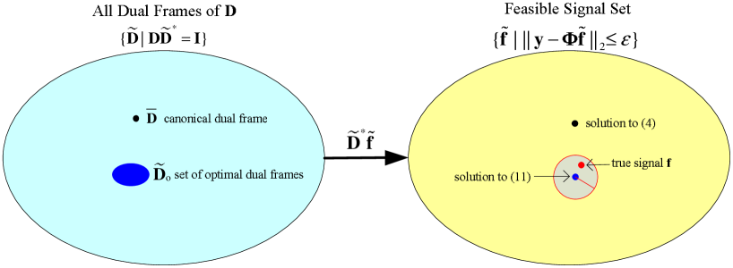
Figure 1: A schematic overview of the family of dual-based $\ell_{1}$-analysis approaches

3 Performance Analysis of $\ell_{1}$-Synthesis

In this section, we present a new performance analysis of the $\ell_{1}$-synthesis approach. We begin by showing that the $\ell_{1}$-synthesis and the optimal-dual-based $\ell_{1}$-analysis approaches are equivalent.

Theorem 2.

$\ell_{1}$-synthesis and optimal-dual-based $\ell_{1}$-analysis are equivalent.

Proof.

We start with the optimal-dual-based $\ell_{1}$-analysis approach as posed in (13). Let $\tilde{{\bf x}}=\bar{{\bf D}}^{*}\tilde{{\bf f}}+{\bf P}{\bf g}$, then we have ${\bf D}\tilde{{\bf x}}=\tilde{{\bf f}}$. Since both $\tilde{{\bf f}}$ and ${\bf g}$ are free, then $\tilde{{\bf x}}\in{\mathbb{R}}^{d}$. Put the two facts into (13), we obtain the $\ell_{1}$-synthesis method (3). On the other hand, we start from the $\ell_{1}$-synthesis formulation. For any $\tilde{{\bf x}}\in{\mathbb{R}}^{d}$, the following decomposition always holds

$$\tilde{{\bf x}} =\tilde{{\bf x}}_{R}+\tilde{{\bf x}}_{N}={\bf D}^{*}({\bf D}{\bf D}^{*})^{-1}{\bf D}\tilde{{\bf x}}+{\bf P}\tilde{{\bf x}}$$

$$=\bar{{\bf D}}^{*}{\bf D}\tilde{{\bf x}}+{\bf P}\tilde{{\bf x}},$$

where $\tilde{{\bf x}}_{R}$ and $\tilde{{\bf x}}_{N}$ are the components of $\tilde{{\bf x}}$ belonging to the row space and the null space of ${\bf D}$, respectively. Define $\tilde{{\bf f}}={\bf D}\tilde{{\bf x}}\in{\mathbb{R}}^{n}$ and ${\bf g}=\tilde{{\bf x}}\in{\mathbb{R}}^{d}$, we can arrive at the optimal-dual-based $\ell_{1}$-analysis approach and the two methods are equivalent. ∎

Remark 1: By taking a geometrical description, it was shown in [16] that any $\ell_{1}$-analysis problem (with full-rank analysis operator) may be reformulated as an equivalent $\ell_{1}$-synthesis one. Our results indicate that the reverse is also true. For a given $\ell_{1}$-synthesis problem, there exist some appropriate analysis operators (e.g., optimal dual frames of ${\bf D}$) such that the corresponding $\ell_{1}$-analysis problem is equivalent to the $\ell_{1}$-synthesis one.

With this equivalence, we now establish the error bound of the $\ell_{1}$-synthesis approach. Since $\tilde{{\bf D}}_{\text{o}}$ is some alternative dual frame of ${\bf D}$, i.e., ${\bf D}\tilde{{\bf D}}_{\text{o}}^{*}={\bf I}$, a direct application of Theorem 1 leads to the following results.

Theorem 3.

Let ${\bf D}$ be a general frame of ${\mathbb{R}}^{n}$ with frame bounds $0<A\leq B<\infty$. Let $\tilde{{\bf D}}_{\text{o}}$ be some optimal dual frame of ${\bf D}$ defined in (14) with frame bounds $0<\tilde{A}_{\text{o}}\leq\tilde{B}_{\text{o}}<\infty$, and let $\rho=s/b$. Suppose

$$\left(1-\sqrt{\rho B\tilde{B}_{\text{o}}}\right)^{2}\cdot\delta_{s+a}+\rho B\tilde{B}_{\text{o}}\cdot\delta_{b}<1-2\sqrt{\rho B\tilde{B}_{\text{o}}}$$ (20)

holds for some positive integers $a$ and $b$ satisfying $0<b-a\leq 3a$. Then the solution $\hat{{\bf f}}$ to (3) (or to (13)) satisfies

$$\|\hat{{\bf f}}-{\bf f}\|_{2}\leq C_{0}\cdot\epsilon+C_{1}\cdot\frac{\|\tilde{{\bf D}}_{\text{o}}^{*}{\bf f}-(\tilde{{\bf D}}_{\text{o}}^{*}{\bf f})_{s}\|_{1}}{\sqrt{s}},$$ (21)

where $C_{0}$ and $C_{1}$ are some constants and $(\tilde{{\bf D}}_{\text{o}}^{*}{\bf f})_{s}$ denotes the vector consisting the largest $s$ entries of $\tilde{{\bf D}}_{\text{o}}^{*}{\bf f}$ in magnitude.

Theorem 3 shows that, under suitable conditions on the sensing matrix, the recovered signal $\hat{{\bf f}}$ by $\ell_{1}$-synthesis is very accurate provided that $\tilde{{\bf D}}_{\text{o}}^{*}{\bf f}$ has rapidly decreasing coefficients. By the optimality of $\tilde{{\bf D}}_{\text{o}}$, one may expect that $\tilde{{\bf D}}_{\text{o}}$ will promote high sparsity in the frame expansion of the signal ${\bf f}$. Indeed, as we shall see in the numerical experiments, $\tilde{{\bf D}}_{\text{o}}$ is much more effective in sparsifying ${\bf f}$ than the canonical dual frame does. Consequently, in comparison to the standard $\ell_{1}$-analysis approach, a better signal recovery is often achieved by $\ell_{1}$-synthesis.

More importantly, this new performance analysis result is capable of explaining examples of successful solutions and fine approximations by the $\ell_{1}$-synthesis approach while the recovered coefficient vector ${\bf x}$ is no where near its true value. Known performance analysis results would not have such capacity.

4 Numerical Results

In this section, we present some numerical experiments to demonstrate the effectiveness of the performance analysis results for $\ell_{1}$-synthesis. In these experiments, we use two types of frames: Gabor frames and a concatenation of the coordinate and Fourier bases. The sensing matrix ${\bf\Phi}$ is a Gaussian matrix with $m=32$, $n=128$. Since the dependence on the noise in the error bound (21) is optimal and for the purpose of clarity, we only consider the noise-free case. Both $\ell_{1}$-analysis and $\ell_{1}$-synthesis problems are solved by the algorithm developed in [22] because the returned auxiliary variable (${\bf P}{\bf g}$) by this algorithm can be used to construct the optimal dual frame $\tilde{{\bf D}}_{\text{o}}$ (19). For completeness of this paper, this algorithm is included in Appendix A. We set $\lambda=\mu=1$, $tol=10^{-12}$, $nInner=5$, and $nOuter=100$ in this algorithm for all experiments.

Example 1: Gabor Frames.   Recall that for a window function $g$ and positive time-frequency shift parameters $\alpha$ and $\beta$, the Gabor frame is given by

$$\{g_{{}_{l,k}}(t)=g(t-k\alpha)e^{2\pi il\beta t}\}_{l,k}.$$ (22)

For many practical applications such as radar and sonar, the received signal $f$ often has the form

$$f(t)=\sum_{k=1}^{s}a_{k}g(t-t_{k})e^{i\omega_{k}t}.$$ (23)

Evidently, $f$ is sparse with respect to a Gabor frame. In this experiment, we construct a Gabor dictionary with Gaussian windows, oversampled by a factor of $30$ so that $d=30\times n=3840$. The tested signal ${\bf f}$ is sparse with respect to the constructed Gabor frame with sparsity $s=\text{ceil}(0.2\times m)=7$. The positions of the nonzero entries of the coefficient vector ${\bf x}$ are selected uniformly at random, and each nonzero value is sampled from standard Gaussian distribution.

Figure 2 (a) shows that when ${\bf D}$ is highly coherent with coherence $\mu({\bf D})=0.9934$, the recovered coefficients by the $\ell_{1}$-synthesis are disappointing (with a relative error $\|\bar{{\bf x}}-{\bf x}\|_{2}/\|{\bf x}\|_{2}=0.9039$). However, the signal recovered by the $\ell_{1}$-synthesis is nevertheless quite acceptable (with a relative error equal to $0.0845$), see Figure 2 (b). This example tells us that a good recovery of the coefficients ${\bf x}$ may be unnecessary to guarantee a fine reconstruction of the signal ${\bf f}$. This phenomenon is explainable by the new performance analysis result, but not by performance results based on the accuracy of the recovery of the coefficient vector ${\bf x}$.

Figure 2 (b) also shows that the signal recovery via $\ell_{1}$-synthesis is much better than that of $\ell_{1}$-analysis (relative error: $0.0845$ vs. $0.3445$). This is because the optimal dual frame $\tilde{{\bf D}}_{\text{o}}$ is much more effective in promoting sparsity in the frame expansion of ${\bf f}$ than the canonical dual frame $\bar{{\bf D}}$ does. Figure 2 (c) compares the largest 100 coefficients (in magnitude) of $\bar{{\bf D}}^{*}{\bf f}$ and $\tilde{{\bf D}}_{\text{o}}^{*}{\bf f}$, where $\tilde{{\bf D}}_{\text{o}}^{*}$ is determined by (19).

Example 2: Concatenations.  When signals of interest are sparse over several orthonormal bases (or frames), it is natural to use a dictionary ${\bf D}$ consisting of a concatenation of these bases (or frames). In this experiment, we consider a dictionary consisting of the coordinate and Fourier bases, i.e., ${\bf D}=[{\bf I},{\bf F}]/\sqrt{2}$. The tested signal ${\bf f}$ is a linear combination of spikes and sinusoids, i.e., ${\bf f}={\bf f}_{1}+{\bf f}_{2}={\bf x}_{1}+{\bf F}{\bf x}_{2}$. The sparsity of both ${\bf x}_{1}$ and ${\bf x}_{2}$ is equal to $4$. Again, the positions of the nonzero entries of both ${\bf x}_{1}$ and ${\bf x}_{2}$ are selected uniformly at random, and each nonzero value is sampled from standard Gaussian distribution.

Figure 3 (a) and (b) show that when ${\bf D}$ is incoherent (with coherence $\mu({\bf D})=1/\sqrt{n}=0.0884$), the $\ell_{1}$-synthesis approach not only recovers the signal ${\bf f}$ but also the coefficient vector ${\bf x}$ accurately.

Figure 3 (b) also shows that $\ell_{1}$-analysis fails in recovering the signal with a relative error at $0.8143$. Such a failure is not surprising since $\bar{{\bf D}}={\bf D}$ is ineffective in sparsifying the true signal ${\bf f}$, see Figure 3 (c). By contrast, $\tilde{{\bf D}}_{\text{o}}^{*}{\bf f}$ decays very quickly, which guarantees the good recovery for the signal by $\ell_{1}$-synthesis.

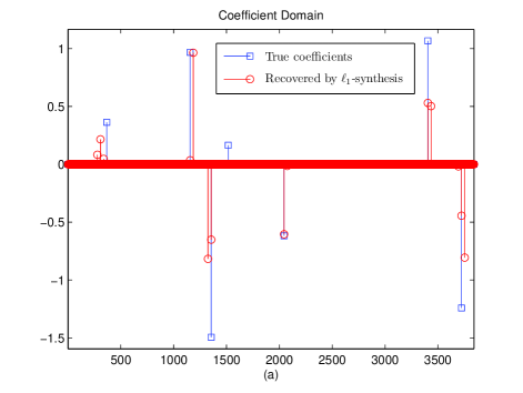
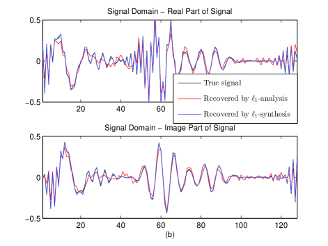
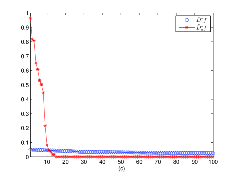
Figure 2: ${\bf D}=$ Gabor frame. (a): recovery in coefficient domain by $\ell_{1}$-synthesis (relative error: $0.9039$) with the relative error defined as $\|\hat{{\bf x}}-{\bf x}\|_{2}/\|{\bf x}\|_{2}$. (b): recovery in signal domain by $\ell_{1}$-analysis (relative error: $0.3445$) and $\ell_{1}$-synthesis (relative error: $0.0845$) with the relative error defined as $\|\hat{{\bf f}}-{\bf f}\|_{2}/\|{\bf f}\|_{2}$. (c): The largest $100$ coefficients of the coefficient vector $\bar{{\bf D}}^{*}{\bf f}$ and $\tilde{{\bf D}}_{\text{o}}^{*}{\bf f}$ in magnitude.

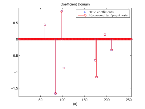
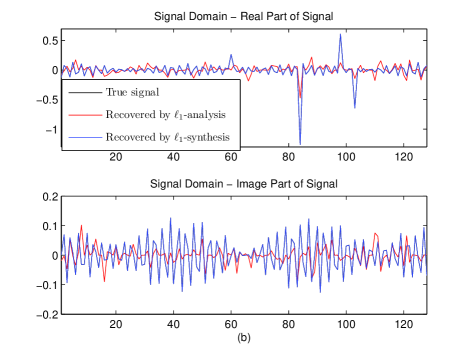
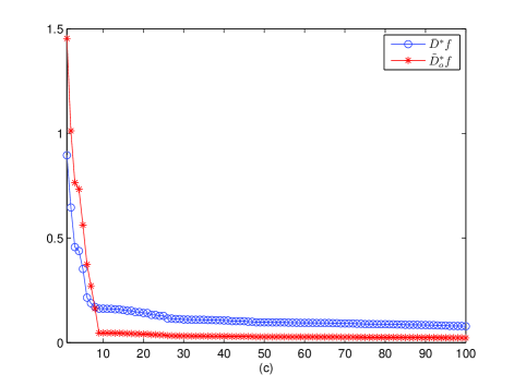
Figure 3: ${\bf D}=[{\bf I},{\bf F}]/\sqrt{2}$. (a): recovery in coefficient domain by $\ell_{1}$-synthesis (relative error: $7.7681\times 10^{-6}$) with the relative error defined as $\|\hat{{\bf x}}-{\bf x}\|_{2}/\|{\bf x}\|_{2}$. (b): recovery in signal domain by $\ell_{1}$-analysis (relative error: $0.8143$) and $\ell_{1}$-synthesis (relative error: $6.7911\times 10^{-6}$) with the relative error defined as $\|\hat{{\bf f}}-{\bf f}\|_{2}/\|{\bf f}\|_{2}$. (c): The largest $100$ coefficients of the coefficient vector $\bar{{\bf D}}^{*}{\bf f}$ and $\tilde{{\bf D}}_{\text{o}}^{*}{\bf f}$ in magnitude.

5 Conclusions

This paper has presented a novel performance analysis for $\ell_{1}$-synthesis in which the dictionary may be highly coherent. Our approach was to show the equivalence between $\ell_{1}$-synthesis and optimal-dual-based $\ell_{1}$-analysis. With this equivalence, the signal recovery error bound for both could be established by using the results in [22]. Finally, the results obtained in this paper were validated via numerical experiments.

Appendix A Split Bregman Iteration for optimal-dual-based $\ell_{1}$-analysis

This appendix includes the split Bregman iteration for optimal-dual-based $\ell_{1}$-analysis in which

• ${\bf f}$: the recovered signal;

• ${\bf x}$: the recovered coefficient vector;

• ${\bf P}{\bf g}$: the auxiliary variable used to construct the optimal dual frame of ${\bf D}$;

• shrink($\cdot$): denotes the element-wise soft shrinkage operation;

• $(\cdot)^{new}$: denotes either $(\cdot)^{k+1}$ if it is available or $(\cdot)^{k}$ otherwise.

Initialization: ${\bf f}^{0}={\bf 0}$, ${\bf x}^{0}={\bf b}^{0}={\bf P}{\bf g}^{0}={\bf 0}$, ${\bf c}^{0}={\bf 0}$, $\mu>0,\lambda>0,nOuter,nInner,tol$;

Output: ${\bf f}$, ${\bf x}$, ${\bf P}{\bf g}$;

while $k<nOuter$ and $\|\mbox{${\bf\Phi}$}{\bf f}^{k}-{\bf y}\|_{2}>tol$ do

       for $n=1:nInner$ do

             ${\bf f}^{k+1}=(\mu\mbox{${\bf\Phi}$}^{*}\mbox{${\bf\Phi}$}+\lambda\bar{{\bf D}}\bar{{\bf D}}^{*})^{-1}[\mu\mbox{${\bf\Phi}$}^{*}({\bf y}-{\bf c}^{k})+\lambda\bar{{\bf D}}({\bf x}^{new}-{\bf P}{\bf g}^{new}-{\bf b}^{new})]$;

             ${\bf x}^{k+1}=\text{shrink}(\bar{{\bf D}}^{*}{\bf f}^{new}+{\bf P}{\bf g}^{new}+{\bf b}^{new},1/\lambda)$;

             ${\bf P}{\bf g}^{k+1}={\bf P}({\bf x}^{new}-\bar{{\bf D}}^{*}{\bf f}^{new}-{\bf b}^{new})$;

             ${\bf b}^{k+1}={\bf b}^{new}+(\bar{{\bf D}}^{*}{\bf f}^{new}+{\bf P}{\bf g}^{new}-{\bf x}^{new})$;

            

       end for

      ${\bf c}^{k+1}={\bf c}^{k}+(\mbox{${\bf\Phi}$}{\bf f}^{k+1}-{\bf y})$;

       Increase $k$;

      

end while

Algorithm 1 Split Bregman Iteration for optimal-dual-based $\ell_{1}$-analysis

References

- [1] R. G. Baraniuk, E. J. Candès, R. Nowak, and M.Vetterli, “Sensing, sampling, and compression,” IEEE Signal Process. Mag., vol. 25, Mar., 2008
- [2] R. G. Baraniuk, E. J. Candès, M. Elad, and Y. Ma, “Applications of sparse representation and compressed sensing,” Proc. IEEE, vol. 98, June, 2010.
- [3] R. G. Baraniuk, M. Davenport, R. DeVore, and M. Wakin, “A simple proof of the restricted isometry property for random matrices,” Constr. Approx., vol. 28, pp. 253–263, 2008.
- [4] A. M. Bruckstein, D. L. Donoho, and M. Elad, “From sparse solutions of systems of equations to sparse modeling of signals and images,” SIAM Rev., vol. 51, pp. 34–81, 2009.
- [5] T. Cai, G. Xu, and J. Zhang, “On recovery of sparse signals via minimization,” IEEE Trans. Inf. Theory, vol. 55, pp. 3388–3397, July, 2009.
- [6] E. J. Candès and T. Tao, “Decoding by linear programming,” IEEE Trans. Inf. Theory, vol. 51, pp. 4203–4215, Dec., 2005.
- [7] E. J. Candès, J. Romberg, and T. Tao, “Stable signal recovery from incomplete and inaccurate measurements,” Comm. Pure Appl. Math., vol. 59, pp. 1207–1223, 2006.
- [8] E. J. Candès and T. Tao, “Near optimal signal recovery from random projections: Universal encoding strategies?,” IEEE Trans. Inf. Theory, vol. 52, pp. 5406–5425, Dec., 2006.
- [9] E. J. Candès, J. Romberg, and T. Tao, “Robust uncertainty principles: exact signal reconstruction from highly incomplete frequency information,” IEEE Trans. Inf. Theory, vol. 52, pp. 489–509, Feb., 2006.
- [10] E. J. Candès, Y. C. Eldar, D. Needell, and P. Randall, “Compressed sensing with coherent and redundant dictionaries,” Appl. Computat. Harmon. Anal., vol. 31, pp. 59–73, 2011.
- [11] S. S. Chen, D. L. Donoho, and M. A. Saunders, “Atomic decomposition by basis pursuit,” SIAM Rev., vol. 43, pp. 129–159, 2001.
- [12] O. Chiristensen, An Introduction to Frames and Riesz Bases. Boston, MA: Birkhäuser, 2003, pp. 87–121.
- [13] D. L. Donoho, “Compressed sensing,” IEEE Trans. Inf. Theory, vol. 52, pp. 1289–1306, Apr., 2006.
- [14] D. L. Donoho, M. Elad, and V. N. Temlyakov, “Stable recovery of sparse overcomplete representations in the presence of noise,” IEEE Trans. Inf. Theory, vol. 52, pp. 6–18, Jan., 2006.
- [15] M. Elad, J. L. Starck, P. Querre, and D. L. Donoho, “Simultaneous cartoon and texture image inpainting using morphological component analysis (MCA),” Appl. Computat. Harmon. Anal., vol. 19, pp. 340–358, 2005.
- [16] M. Elad, P. Milanfar, and R. Rubinstein, “Analysis versus synthesis in signal priors,” Inverse Probl., vol. 23, pp. 947–968, 2007.
- [17] T. Goldstein and S. Osher, “The split Bregman algorithm for L1-regularized problems,” SIAM J. Imag. Sci., vol. 2, pp. 323–343, 2009.
- [18] D. Han, K. Kornelson, D. Larson, and Eric Weber, Frames for Undergraduates. Providence, RI: American Mathematical Society, 2007.
- [19] W. B. Johnson and J. Lindenstrauss, “Extensions of Lipschitz mappings into a Hilbert space,” Contemp. Math, vol. 26, pp. 189–206, 1984.
- [20] F. Krahmer and R. Ward, “New and improved Johnson-Lindenstrauss embeddings via the Restricted Isometry Property,” SIAM J. Math. Anal., vol. 43, pp. 1269–1281, 2011.
- [21] S. Li, “On general frame decompositions,” Numer. Funct. Anal. Optim., vol. 16, pp. 1181–1191, 1995.
- [22] Y. Liu, T. Mi, and S. Li, “Compressed sensing with general frames via optimal-dual-based -analysis,” preprint, 2011. [Online]. Available: http://arxiv.org/abs/1111.4345
- [23] H. Lütkepohl, Handbook of Matrices. New York: Wiley, 1996.
- [24] S. Mallat and Z. Zhang, “Matching pursuits with time-frequency dictionaries,” IEEE Trans. Signal Process., vol. 41, pp. 3397–3415, Dec., 1993.
- [25] H. Rauhut, K. Schnass, and P. Vandergheynst, “Compressed sensing and redundant dictionaries,” IEEE Trans. Inf. Theory, vol. 54, pp. 2210–2219, May, 2008.