Depths of the relief compensation and the anomalous structure of crust and mantle of Mars

Abstract

The contribution to the gravity from the Mars’ relief (topography) and the density jump at the Mohorovicic discontinuity (${\bf M}$) in the quadratic approximation have been derived. The problem of determination of possible depths of compensation for relief’s harmonics of different degree and order have been solved. It is shown, that almost all compensation of a relief is carried out in a range of depths of 0-1400 km. For various relief’s inhomogeneities the compensation is most probable at the depths corresponding to the upper crust ($\bar{d}=4.5\pm 3.7$ km), to crust-mantle transition layer ( $\bar{d}=78\pm 24$ km); to lithospheric boundary ($\bar{d}=200\pm 34$ km); to upper-mean mantle transition layer ($\bar{d}=400\pm 70$ km); to mean-lower mantle transition layer ($\bar{d}=1120\pm 180$ km). The lateral distribution of compensation masses is determined of this depths, and maps are constructed. The possible stresses in crust and mantle of Mars are evaluated. They reach $10^{8}$ Pa. It is shown that relief’ anomalies of volcanic plateau Tharsis and symmetric formation in east hemisphere could arise and be supported dynamically by two plumes of melted mantle substance, enriched by fluids. The plumes have their origins on the boundary depths of lower mantle.

PACS: 96.30. Gc 96.12.-a 96

Keywords: Mars, gravity, isostatic compensation of relief, internal structure, crust, mantle, plumes, planetary dynamics.

1 Introduction

One of riddles of modern planetology is the solution of the question, what forces support significant global variations of a relief heights of terrestrial planets which are under the external gravity field and atmospheric effects should be aligned by the process of denudation. One of the most interesting planets for research of this question is Mars, a range of variations of the Martian surface relief, according to all available information Mars Orbiter Laser Altimeter (MOLA)[1], reaches 44 km, i.e. an order of size 0.013 in comparison with mean planetary radius $R$ = 3389.5 km. For the Earth where the maximum range of variations of the relief heights led to uniform density, is an order 0.002 $R$, it has been shown by us [2], that considerable anomalies of an internal gravitaty field and a field of crust‘s stresses can support existing differences of heights, despite of denudation’s processes. Such considerable gravity anomalous in a crust arise that basically the depth distribution of anomalous masses has a dipolar pattern owing to process of isostatic compensation. So, for example, opposite (in sign) Mohorovicic (M) surface heights anomalies correspond to the relief heights. Especially such conclusion can be fair for Mars, where a range of relief heights variations 10 times more. Therefore, the investigation of the global density structures of Mars and comparison with Earth are of great scientific interest.

Recently there were many observation data as on research of Martian topography [1], and the new models of a Mars gravity field, derived from 5 years of monitoring by Mars Global Surveyor (MGS) [3, 4]. These results have allowed to draw some conclusions about the structure of a Martian crust [5]. So, in [5] the model of surface ${\bf M}$ for Mars (i.e., possible the crust-mantle transition layer ) on the basis of Mars’ gravity after taking into account the contribution of the topography has been constructed. Similarly the ${\bf M}$ model from earlier data has been constructed in [6]. This problem was solved in the linear approximation. However, our similar studies of density structure of the Earth’ crust showed that the linear approximation is insufficient for the accurate accounting of the contribution of the crust boundaries in the internal and external gravitaty fields, it is necessary to take into account the quadratic members [2, 7, 8]. Thus, the account of quadratic members from the relief’ expansion of the degree N brings the additional contribution to harmonics of potential of degree n=0-2N, with this contribution increasing with the growth of n. Especially the account the quadratic terms is essential in dipole (by depth) distribution of anomalous masses. So, if the linear contribution to the external gravitational field is mainly correlated isostatically with relief heights, compensated on M, then the contribution from the account quadratic terms correlates with the squares of heights, i.e., is positive everywhere, both for continents, and for oceans, with its order of magnitude being comparable with the linear contribution. It turned out, that for some regions of the Earth the total contribution has an opposite sign as compared to the linear contribution, which can considerably distort character of the interpretation of satellite data.

In this paper, we consider two methods of obtaining the expansion coefficients of surface ${\bf M}$ for Mars, estimate the contribution of the relief and the density jump (contrast) on ${\bf M}$ to the gravitational field of Mars in the quadratic approximation, we compare the received results among themselves and with the appropriate results for the Earth, and made estimates of the possible distributions of depths of compensation for the relief mass and the density anomalies and that of stresses in the crust and mantle of Mars.

2. The calculation of the contribution from the Mars relief and the density jump at the ${\bf M}$ discontinuity to the gravitaty field in a quadratic approximation

In the linear approximation the laterally distributed anomalous masses are represented as a simple layer of continuous density distributed on a sphere. In this case, there is a linear relation between the coefficients of the expansion of a simple layer density in terms of spherical harmonics and the Stokes constants caused by the the layer’s contribution [2]:

$$\left\{{\Delta C_{nm}^{(s)}}\atop{\Delta D_{nm}^{(s)}}\right\}=\frac{3}{2n+1}\left(\frac{R_{s}}{R_{0}}\right)^{3}\frac{\Delta\sigma_{s}}{\bar{\sigma}}\left(\frac{R_{s}}{a}\right)^{n}\left\{{a_{nm}^{(s)}}\atop{b_{nm}^{(s)}}\right\},$$ (1)

where $\Delta C_{nm}^{(s)}$, $\Delta D_{nm}^{(s)}$ are contributions to Stokes constants; $R_{s}$ is a mean radius of a layer s; $R_{0}=3389.5$ km, $\bar{\sigma}=3.93$ g/cm³ and $a=3396$ km are mean radius, density and mean radius at the equator of the accepted Mars reference ellipsoid, respectively [1, 3];

$\Delta\sigma_{s}H_{s}(\varphi,\lambda)$ = $\Delta\sigma_{s}\cdot\Sigma_{n=1}^{N}\Sigma_{m=0}^{n}(\bar{A}_{nm}^{(s)}\cos m\lambda+\bar{B}_{nm}^{(s)}\sin m\lambda)\bar{P}_{nm}(\sin\varphi)$ is a representation of a simple layers‘ density as expansion series of normalized spherical harmonic of degree $n\leq N$; $\Delta\sigma_{s}$, $H_{s}$ are mean density and layer’s heights relatively to the mean radius $R_{s}$ and $\left\{{a_{nm}^{s}}\atop{b_{nm}^{s}}\right\}=\left\{{a_{nm}}\atop{b_{nm}}\right\}_{1}=1/R_{s}\left\{{\bar{A}_{nm}^{(s)}\atop{\bar{B}_{nm}^{(s)}}}\right\}$ are the normalized spherical harmonic coefficients of $h_{s}=H_{s}(\varphi,\lambda)/R_{s}$. The contribution of layer’s masses to exterior gravitational potential is then defined as follows:

$$\Delta V_{e}(r,\varphi,\lambda)=\frac{fM_{0}}{r}\!\sum\limits_{s}\sum\limits_{n=1}^{N}\!\left(\frac{a}{r}\right)^{n}\!Y_{n}^{(s)}(\varphi,\lambda),$$

$$Y_{n}^{(s)}(\varphi,\lambda)=\sum\limits_{m=0}^{n}(\Delta C_{nm}^{(s)}\cos m\lambda+D_{nm}^{(s)}\sin m\lambda)\bar{P}_{nm}(\sin\varphi).$$

where $M_{0}$ is Martian mass.

In reality the relief masses and especially the anomalous masses, caused by density jump on ${\bf M}$, are not simple spherical layers, but are distributed in height relative to the reference ellipsoid $r_{e}$. In this case the coefficients of development (2) can be found by integration over relief masses:

$$\left\{{\Delta C_{nm}^{(s)}}\atop{\Delta D_{nm}^{(s)}}\right\}=\frac{\Delta\sigma_{s}}{(2n+1)M_{0}}\int\int\int r^{\prime(n+2)}\bar{P}_{nm}(\sin\varphi^{\prime})\cos m\lambda^{\prime}dr^{\prime}d\lambda^{\prime}d\sin\varphi^{\prime},$$

where

$$\int r^{\prime(n+2)}dr^{\prime}=$$

$$\frac{r_{e}^{(n+3)}}{n+3}\left[\left(1+\frac{H_{s}}{r_{e}}\right)^{(n+3)}-1\ \right]\approx R_{s}^{n+3}\left[\frac{H_{s}}{R_{s}}+\frac{n+2}{2}\left(\frac{H_{s}}{R_{s}}\right)^{2}+\alpha(n+2)\frac{H_{s}}{R_{s}}\bar{P}_{2}(\sin\varphi)\right]$$

in a quadratic approximation; $r_{e}=R_{s}(1-\alpha\bar{P}_{2}(\sin\varphi))$; $\alpha=\frac{2}{3}e$; and $e=1/199.5$ is oblateness of the reference ellipsoid, for which value the hydrostatic oblateness [9] was taken.

Therefore, if one takes into account quadratic terms and ellipsoidal structure of reference surface some additional terms arise in formula (1), namely

$$\left\{{a_{nm}^{s}}\atop{b_{nm}^{s}}\right\}=\left\{{a_{nm}}\atop{b_{nm}}\right\}_{1}+\frac{n+2}{2}\left\{{a_{nm}}\atop{b_{nm}}\right\}_{2}+\alpha(n+2)\left\{{a_{nm}}\atop{b_{nm}}\right\}_{3},$$

where the terms in braces $\{\}_{1}$, $\{\}_{2}$, and $\{\}_{3}$ with the subscripts 1, 2, and 3 correspond to the expansion coefficients of the functions $h_{s}$, $(h_{s})^{2}$, and $h_{s}\bar{P}_{2}(\sin\varphi)$ respectively. The formulas expressing the coefficients $\{a_{nm},b_{nm}\}_{2}$ and $\{a_{nm},b_{nm}\}_{3}$, in terms of the linear terms $\{a_{nm},b_{nm}\}_{1}$, have been derived by mathematically simulating symbolic computations in computer algebra systems [7].

Expansion of heights of surface ${\bf M}$ by the first mode ( ${\bf M1}$ model) was obtained by the method of successive approximation procedure. At first step, harmonic coefficients of the Martian potential after taking into account the contribution from the topographic masses into the potential in the quadratic approximation were found, and the expansion coefficients of the heights of ${\bf M}$ in the linear approach were determined on the basis of the obtained coefficients. Having found the contribution to potential of the quadratic members of heights of ${\bf M}$, the new expansion coefficients of heights of ${\bf M}$ in the linear approach again were determined. The process of calculation was repeated to the complete convergence of results .

The expansion coefficients of the surface ${\bf M}$ heights by the second method ( ${\bf M2}$ model) were obtained using the hypothesis of isostatic compensation toopographic heights at ${\bf M}$. Here for all harmonics, we used the same transfer multiplier: $k=\Delta d/\Delta h=(\sigma_{r}/\Delta\sigma_{M})(R_{0}/R_{M})^{3}$, where $\sigma_{r}=2.8$ g/cm³ - is the mean density of the relief’ masses, $\Delta\sigma_{M}=0.6$ g/cm³ - mean density contrast on ${\bf M}$, $\Delta d$ - are the depths of the surface ${\bf M}$ relative to the level surface corresponding to an average depth $\Delta\bar{d}=45$ km ( $R_{M}=3344.5$ km) [5], and $\Delta h$ - the heights of the Martian topographic relative to the hydrostatic ellipsoid, corresponding to $R_{0}=3389.5$ km.

3. Determination of the depths of the compensation of the topographic masses

Since there have been no seismic surveys on Mars, the preliminary data on its internal structure were obtained on the basis of observational data on its gravity and topography, as well as on the basis of some theoretical conclusions [5, 6]. These conclusions are based on cosmogonic scenarios about the formation of terrestrial planets, the geophysical and geochemical information and on high energy physics data.

One of the first tasks at studying of Martian internal structure is to determine of a crust-mantle interface and a possible density jump at ${\bf M}$. The authors of [6], proceeding from a hypothesis about effectively thermal formation of terrestrial planets, come to the conclusion about a possible Martian crustal thickness of 150-200 km and a density contrast of $0.5$ g/cm³. In the same paper, where, on the basis of Bouguer anomalies, the contribution from a relief to a gravity is estimated in the linear approximation, the model of depths ${\bf M}$ relative an average depth level of 140 km is produced. In [10] it is shown, that a crustal thickness can vary in the range of 50-150 km depending on the mineral composition and temperature distribution. In [5], proceeding from petrological and geophysical constraints, concluded that the thickness of a crust is not more than 50 km. In the same paper the authors present the model of depths ${\bf M}$ relative mean depth of 45 km and at the density jump $0.6$ g/cm³. In [4] on the basis of the degree correlation between harmonic coefficients of gravity and topography, the mean level of relief compensation depths of $72\pm 18$ km is obtained.

In the observed works, and also in similar examinations (for example, in [11], where the average depth ${\bf M}$ calculated on the basis of the Airy compensation model for different regions, is equal $90\pm 10$ km), the problem of compensation of relief masses was considered at one level only, the level of ${\bf M}$ discontinuity. However, analogous studies for the Earth [12] show, that in planet’ interiors there can be several compensation levels, consistent with the results obtained from analysis of the Earth’s eigentones and seismological data. Thus depths of compensation for different topography harmonics proved to be strongly dependent on the harmonic degree and order. Therefore our first task was to determine the possible depths of compensation for harmonics of different degrees and orders for expansion of heights of Mars’relief relative to the hydrostatic ellipsoid.

The solution of this problem should satisfy a sistem of two equations, where one of which reflects the consistency between contribution of topographic and compensating masses and the observations, and the other equation reflects the equality of the pressures below the compensation depth to the hydrostatic pressure. The solution obtained for the compensation depth $d_{nm}$ for an arbitrary relief harmonic $a_{nm}$ was defined as a result of the relationship:

$$d_{nm}=R_{0}-R_{M}\left(a_{nm}^{M1}/b_{nm}^{M2}\right)^{1/n},$$

where $a_{nm}^{M1}$ and $a_{nm}^{M2}$ are the expansion coefficients of heights of the surfaces ${\bf M1}$ and ${\bf M2}$ at the fixed value of $R_{M}$ (for relief harmonic $b_{nm}$ the formula is similar with replacement $a_{nm}$ by $b_{nm}$).

As we see, solution (3) is possible, i.e. $d_{nm}\geq 0$ if $0\leq a_{nm}^{M1}/b_{nm}^{M2}\leq(R_{0}/R_{M})^{n}$.

If expansion coefficients of the relative altitudes at ${\bf M}$, received by the first (${\bf M1}$) and second (${\bf M2}$) method, do not satisfy condition (3) for any fixed compensation depth $d_{nm}<R_{0}$, there should be a two-layer compensation. The possible depths of compensation layers are determined then from the analysis of the results obtained for those harmonics for which there exists a solution (3). The final choice is based on the principle of minimization of deviation of the internal structure of Mars from the hydrostatic equilibrium.

4. Results and disscussion

Figure 1: Dependence of the relative mean-square contribution of quadratic members to the planet’s external gravitational potential on the expansion degree $n$ (a)— for the Earth; (b)— for Mars, the ${\bf M1}$ model, and (c)— for Mars, the $\bf M2$ model. Notations: 1— for topographic masses; 2 — for he density jump at $\bf M$; and 3— for the total contribution.

(1) In this study, we used algorithms and formulae that express the expansion coefficients in the spherical functions of the square of some function of $(x=\sin\varphi,\lambda)$, given initially in the form of a similar expansion into spherical harmonics, through the coefficients of this initial expansion [7]. Algorithm developed by us allows to receive these formulae for arbitrary degree $N_{max}$ of initial expansion. The final formulae for numerical calculations are obtained for $N_{max}=9$ inclusive, and they allow one to estimate the contribution of quadratic members into the Stokes constans of the degree $n=0...18$. According to [6], the decomposition to $N=18$ is quite sufficient to identify the main singularities of Martian topography and gravity. We used the contribution of the quadratic terms to the Earth’s and Mars’s gravitational field from the relief masses and the crust-mantle density contrast at ${\bf M}$ to illustrate the results obtained. (Fig1) shows the dependence on $n$ mean-square contributions $\Delta V_{n}=\sqrt{D_{n,2}/D_{n,1}}$ for the relief masses and density jump at ${\bf M}$, both separately and together. Here indexes 1 and 2 correspond to the linear and quadratic members, respectively; $D_{n}=\sum\limits_{m=0}^{n}\left((a_{nm})^{2}+(b_{nm})^{2}\right)$, $a_{nm}$ and $b_{nm}$ are the harmonic coefficients of presented expansion.

A comparison of Figs.1a, 1b, and 1c shows that, for Mars, the contribution of the quadratic terms in the external potential both of topographic masses, and the density jump at ${\bf M}$, on average, 10 times order of magnitude larger than for the Earth, and is comparable to the linear contribution on the order of smallness for 40% of the coefficients. This is especially typical for the ${\bf M2}$ model, for which the quadratic contribution exceeds the linear contribution for 20% of the coefficients ( beginning from $n=1$), while for the Earth, the quadratic contribution exceeds the linear contribution only for a few coefficients from the range under consideration. The distribution histogram for the relative quadratic contribution to the Stokes constants (the ratio of the quadratic terms to linear) reaches its maximum (22% of coefficients) for the relative square contribution equal 0.4 (for the Earth, these figures are 16% and 0.01, respectively [7]).

A comparison of the two arrays of the expansion harmonic coefficients of heights boundary ${\bf M}$ shows, that determination of altitudes of ${\bf M}$ by the first method appears to be incorrect. For example, in [13] for the Earth it is shown, that the conventional practice for determination the ${\bf M}$ depths on the basis of Bouguer anomalies is not confirmed for almost all harmonics of the degree $n>2$ (there is no correlation between the Bouguer anomalies and the ${\bf M}$ depths obtained from seismic data). From this work, and also from [14] follows, that for the Earth the transmission multipliers decrease with the growth of the expansion degree $n$ approximately according to a linear law. Obviously, for a thicker Martian crust (which is three times thicker in comparison with the Earth’s crust) the decreasing law must be more strongly expressed. However, a comparison of the expansion coefficients of the ${\bf M}$ heights obtained by the first and second method shows that the transmission factors, on the average, do not decrease with $n$, and even for some harmonics, they increase. Apparently, the Mars gravity anomalies essentially depend on the inhomogeneous density structures as well as Martian crust, and the deeper layers.

Figure 2: Histograms of the distribution of the compensation depths for topography harmonics with a step of (a) 40 km, (b) 20 km, and (c) 10 km.

(2) Figure 2 presents distribution histograms of the compensation depths of topography harmonics for the entire depth range $0-1500$ km with a step of 40 km (Fig. 2a), 20 km ( Fig. 2b) and more detailed for the depth range $0-390$ km with a step of 10 km ( Fig. 2c), obtained from (3) for $n\leq 18$. The histograms and mean depths were calculated taking into account weights corresponding to the amplitudes of considered topography harmonics. An analysis of the histograms results in the following conclusions: almost all the topography is compensated in the depth range $0-1400$ km, and about 20% of compensation occurs in the upper crust (the depth range $d=0-20$ km, $\bar{d}=4.5\pm 3.7$ km). Further it is possible to identify several main layers of compensation: a boundary interface crust-mantle ($d=50-130$ km, $\bar{d}=78\pm 24$ km); the lithospheric boundary ($d=160-240$ km, $\bar{d}=200\pm 34$ km); upper- middle mantle transition layer ($d=310-470$ km, $\bar{d}=400\pm 70$ km); and middle-lower mantle transition layer ($d=1000-1400$ km, $\bar{d}=1120\pm 180$ km). Note that in each layer the compensation maximum occurs usually near the layer’s boundary. This may speak about variations in the heights of the boundaries separating layers of different densities.

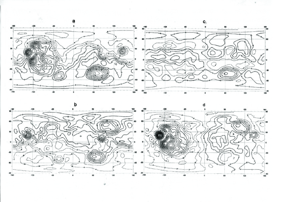
Figure 3: Anomalous structures of the crust of Mars for the expansion to 18 degrees: (a) the height of relief relative to hydrostatic ellipsoid, the isoline cross section is 1 km, the range of variations is ( -7.2, 11.5) km; (b) - density anomalies in the upper crust (at depths of 0 – 20 km), the isoline cross section is 2$\cdot 10^{6}$, the range of variations is ( -13.0,17.5)$\cdot 10^{6}$; (c) – the density anomalies in the boundary layer of crust-mantle (at depths of 50 – 130 km), cross isolines is 2$\cdot 10^{6}$, the range of variations is ( -6.9, 8.4)$\cdot 10^{6}$; (d) nonhydrostatic pressure of the crust on the lithosphere (at depths of 130 km), the isoline cross section is $10^{7}$ Pa, the range of variations is ( -5.4, 14.5)$\cdot 10^{7}$ Pa.

As each relief’ inhomogeneity is characterized by a certain set of harmonics, the maximum concentration of the compensation for this set in a certain range of depths can testify to the most probable depths of compensation of considered relief’ inhomogeneity. Figure 3 and figure 4 present density maps of the compensating masses, recalculated to a densities of a simple layer at mean depths 0, 78, 200, 400, 1120 km corresponding to the set of harmonics for layers with this mean depths. For harmonics for which condition (3) is not fulfilled, two-layer compensation at the selected depths are introduced. In this case for each harmonics and all the possible variants of compensation, we defined the weight function, that is inversely proportional to the sum of absolute values of the density variations, and by taking it into account, we calculated the density anomalies at considered depths. We have used the presented procedure earlier in [12] for determining the density anomalies in the crust and mantle of the Earth at the depths, selected on the basis of seismic data. The obtained density distributions are in good agreement with the results, obtained on the basis of the spectral analysis of the eigenfrequency normal modes for the Earth. The application of this same procedure for Mars allows one to count on the reliability of the obtained results, although this is only a model representation

A comparison of the obtained density distributions allow the following conclusions: (1) the dichotomy of the relief of Mars (Fig. 3a), caused by the first degree harmonics, in the main is compensated by lava filling of the crust of the northern hemisphere plains (Fig 3b); (2) the relief anomalies of the Tharsis volcanic plateau and the symmetrical formation in the eastern hemisphere, caused mostly by second degree harmonics, possibly, may have arisen and are dynamically supported by the presence of two plyumes of the enriched by fluids molten mantle substance, with these plumes having their origin on the upper and lower mantle boundary (Fig. 4c) and decomposing into several branches at the tops of the upper mantle (Figs. 4a, 4b). The penetration of these plumes through the mantle and the lithosphere became possible, apparently, after the impact of the large asteroid, which have led to the topographic dichotomy and the formation of cracks in the crust and mantle, through which the molten substance reached the surface. The lift of the plumes’ light substance was later complicated by the presence of downward flows of the partially cooled heavy substance of lavas in the process of gravitational differentiation (Figs 4a, 4b). Let us note that the ascending current into the mantle, the stronger under the Tharsis, pushes aside around the descending masses, and in the symmetrical equatorial region the stronger downflow pushes aside around the light ascending masses (Fig. 4b). Figure 4b can also be interpreted as the sagging of the lithosphere under Tharsis and its lifting around the plateau, and as the lift of the lithosphere under the symmetrical equatorial region and lowering the surrounding areas, caused by the load pressure of the lithosphere’ masses.

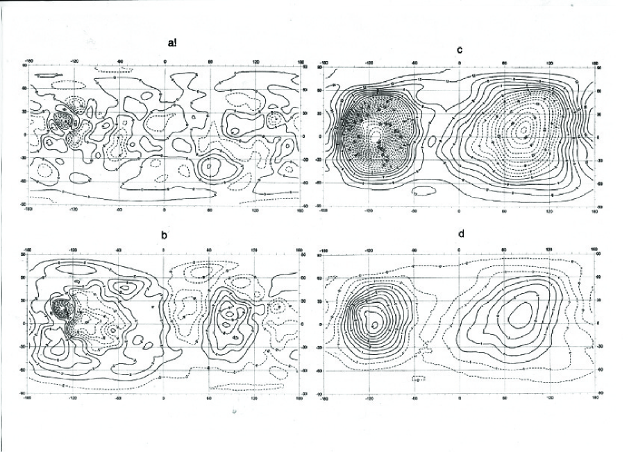
Figure 4: Anomalous structures in Martian mantle for an 18-degree expansion: (a) density anomalies in the lithosphere boundary layer (at a depth of 160 – 240 km); the contour interval is 2$\cdot 10^{6}$ kg/m²; the variation range is (from –11.6 to 6.0)$\cdot 10^{6}$kg/m²; (b) density anomalies in the upper-middle mantle transition layer (at a depth of 310 – 470 km); the contour interval is 2$\cdot 10^{6}$ kg/m²; the variation range is (from –16.3 to 9.5)$\cdot 10^{6}$ kg/m²; (c) density anomalies in the middle-lower mantle transition layer (at a depth of 1000 – 1400 km); the contour interval is 2$\cdot 10^{6}$ kg/m²; the variation range is (from –39.8 to 20.0)$\cdot 10^{6}$ kg/m²; (d) nonhydrostatic pressure in the middle mantle (at a depth of 600 km); the contour interval is $10^{7}$ Pa; the variation range is (from –4.2 to 9.2)$\cdot 10^{7}$ Pa.

Figure 4 shows that the volcanic craters of increased density (Olympus and craters of Tharsis plateau) have their sources in the upper-lower mantle interface layer at depths of $1120\pm 180$ km, Elysium and smaller craters around Hellas Planitia, in the upper mantle at depths of $400\pm 70$ km and at depths of $200\pm 34$ km, small craters between the Tharsis and Argyre, in the crust-mantle transition layer (Figure 3c) at depths of $78\pm 24$ km. The craters of impact origin (Hellas, Isidis, and Argyre), perhaps analogous to the lunar mascons of the increased density, extends down to depths of $200\pm 34$ km and are surrounded by a ring structures with reduced density (Figs 3c , 4a). It is interesting to note the distributions of the density anomalies that are elongated in longitude in the crust- mantle boundary layer (Fig. 3c). Perhaps this is due to the accumulation in this layer of lava and fluid flows from the underlying mantle layers, with different velocity distribution in longitude. These flows can stretch along the longitude also under the influence of Coriolis forces, generated by the convective motions in the mantle near the crust boundaries to the north or south. The regions of negative anomalies, including subpolar areas, may characterize the reserves of fluids, including water, that had not time to reach the surface of Mars through the hardened crust.

It is possible to explain also Figure 3c by the variations in the boundary ${\bf M}$. There is no clear correlation of depths ${\bf M}$ with the structures of relief (with some exception for the Utopia, Elysium, Hellas, Argyre and Alba because of the partial compensation on ${\bf M}$). Under the Great Northern plain, Utopia, Arabia Terra, Terra Sirea, Terra Cimmeria and Prometheus Basin, boundary ${\bf M}$ could be raised under the influence of upward flows from the mantle (Figs 4a,b), under Alba Patera, in the equatorial eastern hemisphere and a southern part of Tharsis it was omitted under the influence of the load pressure of crust.

Nonhydrostatic pressure in different layers of the crust and mantle, produced by the pressure of the overlying layers, reach their maximum of 145 MPa in the lithosphere (Fig. 3d), and decrease and become smoother in the middle mantle (Fig. 4d). They must be balanced by the pressure of the underlayers (because of the isostatic equilibrium condition) and characterize the distribution of the vertical and horizontal stresses (positive values correspond to vertical compressive stresses and horizontal tensile stresses, and vice versa). A comparison of the maps shows that in the Martian mantle, there could have been (or exist till now), the convective motions, which, perhaps, was the source of nonhydrostatic stresses ( within the dynamic approach). The absence of the density and pressure anomalies below the depth of 1400 km shows that the deeper Martian interiors are in a well-established equilibrium, that also leads to the absence of convective motions in the core and, therefore, to the absence of the conditions for a hydromagnetic dynamo.

Conclusions

At an estimating the contribution of the relief’masses and the density jump at ${\bf M}$ (Moho density contrast) to Martian gravity, it is necessary to consider the quadratic members. Eestimating the ${\bf M}$ depths from Bouguer anomalies, which is consistent with the hypothesis of the homogeneous structure of the Martian crust, contradicts the data of the analysis of transmitting coefficients for Mars and the analodous estimates for the Earth. The Martian crust and mantle are characterized by a nonhomogeneous distribution of density and stresses down to the depth 1400 km. The topographic anomalies of the Tharsis volcanic plateau and the symmetrical formation in the eastern hemisphere, possibly, have arisen, and be dynamically supported by two plumes of melted mantle substance, enriched by fluids. The plumes have their origins at the boundary of the lower mantle.

References

- [1] M.T. Zuber, S.T. Solomon, R.J. Phillips et al ., Science 287 1788 ( 2000)
- [2] N.A. Chujkova, L.P. Nasonova and T.G. Maximova, Vestn. Mosk. Univ., Fiz. Astron., 4, 48 (2006)
- [3] D.N. Yuan , W.L. Sjogren, A.S. Konopliv et al., J. Geophys. Res. 106 23377 ( 2001)
- [4] A.S. Konopliv., C.F. Yoder, E.M.Standish et al., Icarus. 182 .23. (2006)
- [5] G.A. Neumann, M.T. Zuber, M.A. Wieczorek et al., J.Geophys. Res. 109. doi:10.1029/ 2004JE002262. E08002. ( 2004)
- [6] V.N. Zarkov, E.M.Koshliakov and K.I. Marchenkov, Astron. Vestn. (Engl. transl. Solar System Research)25, No 2 3 515 (1991)
- [7] L.P. Nasonova and N.A. Chuikova, Vestn. Mosk. Univ., Fiz. Astron., No. 6, 61 (2007) [Moscow Univ. Phys. Bull. 62, 248 (2007)].
- [8] N. A. Chujkova, L. P. Nasonova, and T. G. Maximova, Astron. Astrophys. Trans.26, (4, 5), 391 (2007).
- [9] V.N. Zarkov and T.V. Gudkova, Astron. Vestn. (Engl. transl. Solar System Research) 27, No 2 3 (1993)
- [10] A.IU. Babeiko, C.V. Sobolev and V.N. Zarkov, Astron. Vestn.(Engl. transl. Solar System Research) 27, N 2 55 (1993)
- [11] D.L.Turcotte, R. Sheherbakov R., B.D.Malamud. et al. , J.Geophys. Res. 107 1 (2002)
- [12] N.A. Chuikova, and T.G. Maksimova, Vestn. Mosk. Univ., Fiz. Astron., No. 2, 67 (2010) [Moscow Univ. Phys. Bull. 65, N 2 137 (2010)].
- [13] N.A. Chujkova, A. N. Grushinsky and T.G. Maximova, SAI Proceeding. 65 51 (1996)
- [14] N.A. Chujkova, S.A. Kazarjan and T.G. Maksimova, Vestn. Mosk. Univ.,Fiz. Astron. 2 55 (2003)