ABSTRACT

We compute the canonical partition function for quantum black holes in the approach of Loop Quantum Gravity (LQG). We argue that any quantum theory of gravity in which the horizon area is built of non-interacting constituents cannot yield qualitative corrections to the Bekenstein-Hawking (B-H) area law, but corrections to the area law can arise as a consequence additional constraints inducing interactions between the constituents. In LQG this is implemented by requiring spherical horizons. The canonical approach for LQG seemingly favours a logarithmic correction to the B-H law with a coefficient of $-\frac{1}{2}$. Our initial calculation of the partition function uses certain approximations that, we show, do not qualitatively affect the expression for the black hole entropy. We later discuss the quantitative corrections to these results when the simplifying approximations are relaxed and the full LQG spectrum is dealt with. We show how these corrections can be recovered to all orders in perturbation theory. However, the convergence properties of the perturbative series remains unknown for now.

Keywords: Loop Quantum Gravity, Black Hole Thermodynamics, Barbero-Immirizi Parameter.

I Introduction

Classical and semi-classical properties of black holes have been studied quite vigorously in past several decades CLSBH . As a result, we have discovered that some nice thermodynamic properties can be associated with them. For example, black holes are now understood to be endowed with a temperature and to possess an entropy characterized by their mass and by any other charges that may be associated with them. These properties, although derived on the semi-classical level, are expected to be robust enough that explaining them in terms of an ensemble of microstates has come to be considered of prime importance for any quantum theory of gravity. Many approaches to quantum gravity, like String theory ST , Loop Quantum Gravity (LQG) LQG and the theory of Causal Sets CST , have therefore taken up this problem and each has succeeded in some measure in providing some deeper insight into the problem. However, the Bekenstein-Hawking area law seems generic enough that all the approaches, although differing considerably in design, are able to reproduce it. As a result, there remains no general consensus on a final theory of quantum gravity and it becomes essential to attempt not only to obtain the original semi-classical results, but also to discover, if possible, signature corrections of quantum origin to the semi-classical wisdom.

In this paper, we take up one of the popular approaches to quantum gravity, namely LQG. Black holes have been studied quite extensively in this approach LQGBH1 , mostly in context of isolated horizon scheme BHasIH . In LQG, the area spectrum of an isolated horizon is readily available and black holes with a given horizon area have been studied in the microcanonical ensemble Rovelli ; Kaul ; gm05 ; gm06 . Logarithmic corrections to the Bekenstein-Hawking entropy have been shown to exist on the semi-classical level sclog and as a signature of LQG gm05 ; gm06 . They have been proposed in other approaches as well logterms but there is some confusion about the precise value of the coefficient of this term. Approaches that employ conformal symmetry techniques generally seem to prefer the value $-3/2$ whereas the pure quantum geometry approach seems to favor the value of $-1/2$.

We analyze LQG black holes in the canonical area ensemble with a finite number of punctures, $N$. The use of the area ensemble was first advocated in Krasnov and has since been employed by others (see, for eg. bv11 ; bv11a and references therein). A justification for its use has recently been proposed in fgp11 . The use of $N$ as a statistical variable in the area canonical ensemble was first advocated in m01 and its importance for black holes was emphasized in gp11 . There are similarities between our approach and that of gm06 and our canonical calculation agrees with the results therein, although the latter work was performed in the microcanonical ensemble. The microcanonical and canonical entropies do not have to coincide, of course, except in the thermodynamic limit. Now it is well known that the microcanonical entropy in LQG suffers from the fact that the black hole entropy is not a differentiable function of its arguments but rather a ladder (or staircase) function cdf07 ; bv11 ; pp11 . As pointed out in bv11a , this makes it difficult to interpret basic thermodynamic variables, such as the temperature, which are defined in terms of derivatives of the entropy. The canonical partition function is assumed to be, by contrast, a smooth function of its arguments. We obtain the canonical partition function without making any assumptions concerning our variables or referring to any semi-classical feature, so the following analysis is independent of any à priori thermodynamic input. We expect that our approach will provide a useful framework for examining area fluctuations about the microcanonical value and for a generalization to the grand canonical ensemble, where we should be able to precisely test some of the assumptions of gm06 ; gp11 . Here, we find general agreement with gm06 .

In section II we briefly review the LQG approach to black holes. We begin our computation of the canonical partition function in section III by making a certain approximation, which we will refer to as the “shell” approximation and define later, to the LQG area spectrum. Ignoring the projection constraint, we easily recover the Bekenstein-Hawking area-entropy relation together with an estimate of the Barbero-Immirizi parameter and we show that any correction to the Bekenstein-Hawking entropy is inherently absent. In section IV we impose the sphericity (or projection) constraint on the black hole horizon and re-evaluate the partition function. The effect of the projection constraint is to produce a logarithmic correction to the standard semi-classical result. Section V is devoted to a discussion on relaxing the “shell” approximation and incorporating the full LQG spectrum in a perturbative fashion. We develop a systematic approach to compute the corrections to all orders. We conclude by discussing some issues raised as well as the general outlook related to our approach in section VI.

II Black Holes in LQG

As a non-perturbative, background independent approach to canonical quantum gravity, Loop Quantum Gravity (LQG) has met many challenges effectively, although a full dynamical picture of quantum gravity has remained elusive so far. Starting with holonomies, built from su(2) valued connections, and fluxes, built from densitized triads, as basic variables of the theory, one obtains a well-defined Hilbert space made up of cylindrical functions acting on spin-networks over which the holonomies and densitized triads are defined. A spin-network is a graph with edges labeled with su(2) representations and nodes characterized by su(2) intertwiners. Spin-networks are eigenstates of the Area and Volume operators and this leads to a reasonably good description of some of the geometrical observables of the theory, at least on the kinematical level. For example, an edge with spin-representation $j$ carries an area of eigenvalue

$$A_{j}=8\pi\gamma\l_{p}^{2}\sqrt{j(j+1)},$$ (1)

where $j\in\{\frac{1}{2},1,\frac{3}{2},\ldots\}$ and $\gamma$ is an unknown parameter of quantization known as Barbero-Immirizi parameter. Alternatively, an area element of area $A_{j}$ can be thought as being punctured by an edge of the spin-network carrying representation $j$. In general a surface that is punctured by many edges of different representations will have the area spectrum

$$A=8\pi\gamma\l_{p}^{2}\sum_{i}\sqrt{j_{i}(j_{i}+1)},$$ (2)

where the sum is over all intersections of the edges with the surface. One considers the black hole horizon as an isolated horizon Ashtekar which is threaded by many edges of a spin-network. Each edge carries some representation and hence deposits some area to the horizon as shown in figure 1.

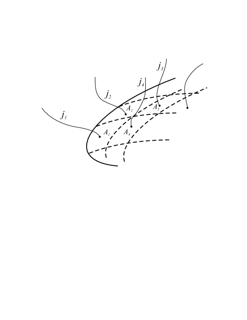
Figure 1: Horizon punctured by the edges of a spin-network

In the microcanonical ensemble, one simply tries to count the number of different configurations, i.e., the different ways of threading a horizon with a fixed area $A$ by spin-representations. This then gives the black hole entropy. However, counting the total number of microstates in this way has not been trivial owing to the fact that the area spectrum in (2) is non-distributive in nature. This issue has been discussed and treated in different ways by various authors Rovelli ; gm05 ; Kaul . In this way, one obtains the asymptotic formula

$$S_{BH}=\frac{\lambda A(\gamma)}{4l_{P}^{2}},$$ (3)

where we have put the Barbero-Immirzi parameter explicitly in the area as it appears in the expression (2) for the area, and utilizes the flexibility of fixing $\gamma$ to recover the Bekenstein-Hawking result.

In the following two sections we will examine LQG black holes in the canonical ensemble. We begin by making the “shell” approximation at first, but later, in section V, we generalize to the full LQG spectrum. This leads to corrections to the entropy derived in sections III and IV but these corrections amount to a renormalization of the Barbero-Immirzi parameter and do not change the functional dependence of the canonical partition function on the extensive variables.

III Setup for the canonical calculation

Let us begin by first ignoring the projection constraint and, since all punctures are considered to be distinguishable, let us assume that there are $n_{j}$ punctures carrying spin $j$, then

$$A=8\pi\gamma l_{p}^{2}\sum_{j}n_{j}\sqrt{j(j+1)}\equiv 8\pi\gamma\sum_{j}n_{j}a_{j},$$ (4)

with $a_{j}$ capturing the information about the area spectrum. For a configuration containing $N$ distinguishable punctures, $n_{j}$ of which carry spin $j$, we will have

$$\frac{N!}{\prod_{j}n_{j}!}\prod_{j}(2j+1)^{n_{j}}$$

distinct configurations. The degeneracy factor $(2j+1)^{n_{j}}$ signifies $2j+1$ values for $m_{j}=\{-j,-j+1,..,j\}$ for a spin-representation $j$. Therefore, we may write the partition function as

$$Z(\beta,N)=\sum_{\{n_{j}\}}\frac{N!}{\prod_{j}n_{j}!}\prod_{j}(2j+1)^{n_{j}}e^{-8\pi\gamma\beta n_{j}a_{j}},$$ (5)

where $\beta$ is conjugate to the area and is not the black hole temperature. By the Binomial theorem, this is

$$Z(\beta,N)=\left(\sum_{j}(2j+1)e^{-8\pi\gamma\beta a_{j}}\right)^{N}.$$ (6)

Now, since $j\in\{\frac{1}{2},1,\frac{3}{2},\ldots\}$ it is convenient to make the change $2j=l$ so that

$$Z(\beta,N)=\left(\sum_{l=1,2,\ldots}(l+1)e^{-\sigma\sqrt{l(l+2)}}\right)^{N}=z^{N}(\sigma)$$ (7)

where $\sigma=4\pi\gamma l_{p}^{2}\beta$. We will now study the general properties of this kind of partition function without restricting ourselves to to this or any particular area spectrum.

III.1 Formal Solution

If, as we have above,

$$Z(\sigma,N)=z^{N}(\sigma)$$ (8)

then, because $A=-\frac{\partial\ln Z}{\partial\beta}$, it follows that

$$\frac{A}{4\pi\gamma l_{p}^{2}N}=-\frac{\partial\ln z(\sigma)}{\partial\sigma}~{}\stackrel{{\scriptstyle\text{def}}}{{=}}~{}q.$$ (9)

Inverting this relation, one finds a solution of the form

$$\sigma=4\pi\gamma l_{p}^{2}\beta=\sigma(q).$$ (10)

The entropy of the system is obtained from

$$S=\ln Z(\sigma,N)+\beta A(\sigma,N)=N[\ln z(\sigma)+\beta a(\sigma)]$$ (11)

where, $\beta=\beta(q)$ as above and $A=Na$ i.e., $a=4\pi\gamma l_{p}^{2}q,$ as can be seen from (9). Thus,

$$S(q)=N\left[\ln z\{\sigma(q)\}+q\sigma(q)\right].$$ (12)

Now let us maximize the entropy with respect to the total number of constituents (punctures for the LQG model), $N$. Then

$$\frac{S}{N}+N\left(\frac{\partial\ln z}{\partial\sigma}\sigma^{\prime}+\sigma+q\sigma^{\prime}\right)\frac{\partial q}{\partial N}=0,$$ (13)

where the prime refers to a derivative with respect to $q$. Now from (9),

$$\frac{\partial q}{\partial N}=-\frac{A}{4\pi\gamma l_{p}^{2}N^{2}}=-\frac{q}{N},$$ (14)

so,

$$\frac{S}{N}-q\left[\frac{\partial\ln z}{\partial\sigma}\sigma^{\prime}+\sigma+q\sigma^{\prime}\right]=0,$$ (15)

and, since

$$\frac{\partial\ln z}{\partial\sigma}=-\frac{A}{4\pi\gamma l_{p}^{2}N}=-q,$$ (16)

we have

$$\frac{S}{N}-q\sigma(q)=0$$ (17)

or

$$\ln z\{\sigma(q)\}=0\Rightarrow z\{\sigma(q)\}=1.$$ (18)

We must solve this equation for $N=N(A)$ and reinsert into $S$ to determine the entropy as a function of area. In this way we will get

$$S=\left.N(A)q\sigma(q)\right|_{z\{\sigma(q)\}=1},$$ (19)

but the relation $z\{\sigma(q)\}=1$ implies that $q=q_{0}$, a constant. This gives

$$N(A)=\frac{A}{4\pi\gamma l_{p}^{2}q_{0}},$$ (20)

and

$$S=\sigma(q_{0})\frac{A}{4\pi\gamma l_{p}^{2}}.$$ (21)

The entropy is always proportional to the area so long as the canonical partition function obeys (8) and regardless of the spectrum. It follows that any theory of quantum gravity in which non-interacting constituents make up the horizon (like the punctures in LQG at this level) will result in the Bekenstein-Hawking area-entropy law. To obtain the Bekenstein-Hawking relation in LQG framework, the value of the Immirizi parameter should be fixed at

$$\gamma=\frac{\sigma(q_{0})}{\pi}.$$ (22)

Within this framework, any correction (in particular logarithmic) must arise from additional constraints (such as the projection constraint in LQG) on the horizon. Therefore, we do not expect any logarithmic correction to Bekenstein-Hawking relation in shell collapse scenarios vw01 . Now we estimate the numerical value for $\gamma$ for an approximated LQG spectrum, which looks very much like the spectrum in dust shell collapse.

III.2 The ‘Shell” approximation to the LQG spectrum

We define the “shell” approximation by $\sqrt{l^{2}+2l}=\sqrt{(l+1)^{2}-1}\approx l+1$. We have called this the “shell” approximation because an identical solution is obtained in the canonical quantization of the LTB dust models vw01 . In those models the collapsing dust ball is viewed as made up of dust shells, and the apparent horizon for each shell is shown to have a similar area spectrum. In making this approximation, we will be making errors towards low spin punctures, but for large spin punctures, the errors will not be that significant. Then,

$$z(\sigma)=\sum_{l=1,2,\ldots}(l+1)e^{-\sigma(l+1)}=-\frac{\partial}{\partial\sigma}\sum_{l=0}^{\infty}e^{-\sigma(l+2)}=\frac{2-e^{-\sigma}}{(e^{\sigma}-1)^{2}},$$ (23)

so that the condition $z\{\sigma(q)\}=1$ translates to

$$2-e^{-\sigma}=(e^{\sigma}-1)^{2}.$$ (24)

There are two possible solutions for $e^{\sigma}$, viz.,

$$e^{\sigma}=\left\{\begin{matrix}2.247\cr 0.555\end{matrix}\right.$$ (25)

and the equation for $q$

$$q=-\frac{\partial\ln z}{\partial\sigma}=2+\frac{2}{e^{\sigma}-1}+\frac{1}{1-2e^{\sigma}},$$ (26)

determines $q_{0}$ in terms of these solutions. There is only one positive solution for $q$ and it corresponds to $e^{\sigma}=2.247$; we end up with

$$\sigma(q_{0})=0.810,~{}~{}q_{0}=3.318,~{}~{}\gamma=0.258,$$ (27)

using (22). It is important to note that even if an exact calculation could be done then the entropy would still be proportional to $A$ while the constants $q_{0}$ and $\gamma$ would change. Now, for the estimate of the Barbero-Immirizi parameter from microcanonical counting, Ghosh and Mitra, in their study of LQG black holes gm05 , suggest that the correct value for $\gamma$ is $0.274$. On the other hand, Ling and Zhang produce a very similar value, $\gamma\approx 0.247$, from their study LZ of $N=1$ super-symmetric LQG black holes. Importantly, this value of the parameter $\gamma$ is closely related to the agreement between LQG spectrum and quasi-normal (ringing-) mode frequency of black holes Rovelli . One can in principle, get a better estimate for $\gamma$ by dropping the “shell” approximation. We will illustrate how this can be done in section V.

For the present we recall that the projection constraint is still missing and in the next section we will introduce it. This constraint has been identified gm06 as the possible source of a logarithmic correction from analyses in the microcanonical ensemble. First we write the canonical partition function with this constraint, but still staying within the “shell” approximation.

IV The Projection Constraint

We now consider a spherically symmetric black hole. Such a system in LQG will be described by a spin-network which is an eigenstate of the projection operator $\hat{n}\cdot\vec{J}$ with zero eigenvalue. In other words, the $m_{j}$ values carried by the spins puncturing the horizon must add up to zero. This is the projection constraint. It can be written as,

$$\sum_{j,m_{j}}n_{jm_{j}}m_{j}=0,$$ (28)

where $n_{jm_{j}}$ gives the number of punctures carrying spin $j$ and projection $m_{j}=-j,-j+1,\ldots,j-1,j$ along the $z-$axis. We can see that the punctures are now “interacting” in the sense they have to satisfy a constraint for getting the desired quantum state and their interaction will manifest itself in terms of some correction to (21).

First we write,

$$2\sum_{j,m_{j}}n_{jm_{j}}m_{j}=p,$$ (29)

for some integer $p,$ then we will put the constraint on $p$, forcing it to vanish. Suppose there are $N=\sum_{j,m_{j}}n_{jm_{j}}$ punctures, then the partition function becomes

$$Z(\beta,N)=\sum_{\{n_{jm_{j}}\}}\frac{N!}{\prod_{jm_{j}}n_{jm_{j}}!}~{}\delta_{p,0}~{}e^{-8\pi\gamma\beta\sum_{jm_{j}}n_{jm_{j}}a_{j}},$$ (30)

where $\delta_{p,0}$ is the Kronecker delta function. We want a suitable representation for this function. For integer $p$ a convenient representation is

$$\delta_{p,0}=\frac{1}{2\pi}\int_{0}^{2\pi}dk~{}e^{ikp}.$$ (31)

and using it we find

$$Z(\beta,N)=\frac{1}{2\pi}\sum_{\{n_{jm_{j}}\}}\frac{N!}{\prod_{jm_{j}}n_{jm_{j}}!}\left(\int_{0}^{2\pi}dke^{2ik\sum_{jm_{j}}n_{jm_{j}}m_{j}}\right)e^{-8\pi\gamma\beta\sum_{jm_{j}}n_{jm_{j}}a_{j}}.$$ (32)

Interchanging the sum over $n_{jm_{j}}$ and the integral over $k$,

$$Z(\beta,N) = \frac{1}{2\pi}\int_{0}^{2\pi}dk\sum_{\{n_{jm_{j}}\}}\frac{N!}{\prod_{jm_{j}}n_{jm_{j}}!}e^{2ik\sum_{jm_{j}}n_{jm_{j}}m_{j}}e^{-8\pi\gamma\beta\sum_{jm_{j}}n_{jm_{j}}a_{j}},$$ (33)

$$= \frac{1}{2\pi}\int_{0}^{2\pi}dk\left(\sum_{jm_{j}}e^{(2ikm_{j}-8\pi\gamma\beta a_{j})}\right)^{N},$$ (35)

again after using the Binomial theorem. Note that to recover the result with no projection constraint, we must drop the integration over $k$ and set $k=0$. Now let $2j=l$ as before, $2m_{j}=r_{l}\in\{-l,-l+2,\ldots,l-2,l\}$ and consider the sum in the integrand first,

$$\sum_{l=1}^{\infty}\left(\sum_{r_{l}}e^{ikr_{l}}\right)e^{-\sigma\sqrt{l(l+2)}}=\sum_{l=1}^{\infty}\frac{e^{ik(l+2)}-e^{-ikl}}{e^{2ik}-1}e^{-\sigma\sqrt{l(l+2)}}.$$ (36)

We easily check that the limit as $k\rightarrow 0$ of the sum is

$$\lim_{k\rightarrow 0}\frac{e^{ik(l+2)}-e^{-ikl}}{e^{2ik}-1}=l+1,$$ (37)

and therefore (36) reduces to (7).

We want to get the partition function

$$Z(\beta,N) = \frac{1}{2\pi}\int_{0}^{2\pi}dk\left(\frac{1}{e^{2ik}-1}\sum_{l=1}^{\infty}e^{-\sigma\sqrt{l(l+2)}}\{e^{ik(l+2)}-e^{-ikl}\}\right)^{N},$$ (38)

$$\approx \frac{1}{2\pi}\int_{0}^{2\pi}dk\left(\frac{1}{e^{2ik}-1}\sum_{l=1}^{\infty}e^{-\sigma(l+1)}\{e^{ik(l+2)}-e^{-ikl}\}\right)^{N},$$ (40)

$$= \frac{1}{2\pi}\int_{0}^{2\pi}dk\left(\frac{1}{e^{2ik}-1}\sum_{l=0}^{\infty}e^{-\sigma(l+2)}\{e^{ik(l+3)}-e^{-ik(l+1)}\}\right)^{N},$$ (42)

into a manageable form. In the second step, we made use of shell approximation to simplify the calculation. After a little manipulation, we end up with the expression

$$Z(\beta,N)=\frac{1}{2\pi}\int_{-\pi}^{\pi}dk\left(\frac{2\cos k-e^{-\sigma}}{e^{2\sigma}-2e^{\sigma}\cos k+1}\right)^{N},$$ (43)

where we have made use of the evenness of the integrand to rewrite the limits of the integration. Note that this is not of the form (8) and that this is because of the projection constraint, which introduced an interaction between punctures as discussed above. In the limit as $k\rightarrow 0$, the integrand approaches

$$\frac{2-e^{-\sigma}}{(e^{\sigma}-1)^{2}},$$ (44)

which is precisely (23) as required.

Now we try to approximate the integral from the information we have about the integrand. First, we see that it is a unimodal symmetric distribution between its limits. So we would like to approximate it by a “bell-curve”. (In order to do so, we can make the transformation

$$k=2\tan^{-1}(x/2),$$ (45)

to get the limits form $-\infty$ to $\infty$.) We then make an assumption that it is well-approximated by a Gaussian in some regime of $N$. If true, then the variance ($\tilde{\sigma}^{2}$) of the “bell-curve” is obtained by the second derivative of the integrand at the peak, since in the case of a Gaussian

$$\tilde{\sigma}^{2}=-\frac{f(x)|_{0}}{f^{\prime\prime}(x)|_{0}}.$$ (46)

In our case,

$$f(x)=\frac{1}{2\pi}\left(\frac{2\cos k(x)-e^{-\sigma}}{e^{2\sigma}-2e^{\sigma}\cos k(x)+1}\right)^{N}\left|\frac{dk}{dx}\right|,$$

$$=\frac{1}{2\pi(1+x^{2}/4)}\left(\frac{2\cos k(x)-e^{-\sigma}}{e^{2\sigma}-2e^{\sigma}\cos k(x)+1}\right)^{N},$$ (47)

resulting in the variance

$$\tilde{\sigma}^{2}=-\frac{f(x)|_{0}}{f^{\prime\prime}(x)|_{0}}=\frac{2(e^{\sigma}-1)^{2}(2e^{\sigma}-1)}{-1+e^{\sigma}(4+e^{\sigma}(-5+e^{\sigma}(2+4N)))},$$ (48)

which in large $N$ limit tends to

$$\lim_{N\rightarrow\infty}\tilde{\sigma}^{2}\rightarrow\frac{(e^{\sigma}-1)^{2}(2-e^{-\sigma})}{2e^{2\sigma}N}.$$ (49)

Now, being a symmetric distribution its skewness is already zero. We analyze its kurtosis next. For a Gaussian with a zero mean, the kurtosis obtained from fourth standardized moment, can be given by its distribution function as

$$\beta_{2}=\frac{\mu_{4}}{\tilde{\sigma}^{4}}=\frac{f(x)|_{0}f^{(4)}(x)|_{0}}{[f^{\prime\prime}(x)|_{0}]^{2}}=3,$$ (50)

which gives the “excess kurtosis” as

$$\beta_{2}-3=0.$$ (51)

For our case, also due to the fact that its mean is zero, we obtain,

$$\frac{\mu_{4}}{\tilde{\sigma}^{4}}=\frac{f(x)|_{0}f^{(4)}(x)|_{0}}{[f^{\prime\prime}(x)|_{0}]^{2}}=\frac{6[(1-2e^{\sigma})^{2}(e^{\sigma}-1)^{4}+8e^{3\sigma}(-1+e^{\sigma}(2+e^{\sigma}(e^{\sigma}-1)))N+8e^{6\sigma}N^{2}]}{[-1+e^{\sigma}(4+e^{\sigma}(-5+e^{\sigma}(2+4N)))]^{2}}$$ (52)

and we see that in limit of large $N$, the excess kurtosis of this distribution also vanishes,

$$\lim_{N\rightarrow\infty}\frac{\mu_{4}}{\tilde{\sigma}^{4}}-3\rightarrow 0.$$ (53)

For large $N$ the integrand tends to a unimodal symmetric distribution with zero skewness and vanishing excess kurtosis. Thus, our initial assumption is justified and in the large $N$ limit this function is indeed well approximated by a Gaussian. In this limit the partition function is given by the area of a gaussian, which can be readily evaluated. Therefore, we have the partition function in the thermodynamic limit

$$Z(N,\sigma)=f(x)|_{0}\sqrt{2\pi}\tilde{\sigma}.$$ (54)

or, explicitly,

$$Z(N,\sigma)=\sqrt{\frac{(e^{\sigma}-1)^{2}(2-e^{-\sigma})}{2e^{2\sigma}N}}\left(\frac{2-e^{-\sigma}}{(e^{\sigma}-1)^{2}}\right)^{N},$$ (55)

and thus,

$$\ln Z\approx N\ln z(\sigma)-\frac{1}{2}\ln N+\text{const.},$$ (56)

(assuming that $N$ is large) where $z(\sigma)$ is given in (23). We find, as before,

$$\frac{A}{4\pi\gamma l_{p}^{2}N}=-\frac{\partial\ln z}{\partial\sigma}~{}\stackrel{{\scriptstyle\text{def}}}{{=}}~{}q,$$ (57)

and

$$S=\ln Z+\beta A=N[\ln z(\sigma)+\sigma q]-\frac{1}{2}\ln N+\text{const.},$$ (58)

Now

$$\frac{\partial S}{\partial N}=\ln z-\frac{1}{2N}\approx\ln z=0.$$ (59)

for large $N$ and retaining terms up to the order of $1/\sqrt{N}$. This implies, once again, that $z(\sigma)=1,$ and it can be solved for $q_{0}$ and $\sigma(q_{0})$ as before. Then

$$S\approx q_{0}\sigma(q_{0})N(A)-\frac{1}{2}\ln N(A)+\text{const.},$$ (60)

with $N=A/4\pi\gamma l_{p}^{2}q_{0}$, i.e.,

$$S\approx\frac{\sigma(q_{0})A}{4\pi\gamma l_{p}^{2}}-\frac{1}{2}\ln\left(\frac{A}{4\pi\gamma l_{p}^{2}q_{0}}\right)+\text{const.},$$ (61)

or with the chosen value of the Immirizi parameter

$$S=\frac{A}{4l_{p}^{2}}-\frac{1}{2}\ln\left(\frac{A}{4l_{p}^{2}}\right)+\text{const.}$$ (62)

Thus we obtain a logarithmic correction, whose origin lies clearly in the imposition of the projection constraint. The logarithmic correction comes with a factor $-\frac{1}{2}$, as already pointed out in gm05 ; gm06 , and therefore the canonical calculations are shown agree with the microcanonical results. The microcanonical ensemble and the canonical ensemble agree even at the subdominant correction, in contrast with the results of bv11a , in which the coefficient is determined to be $+\frac{1}{2}$. The reason for this discrepancy is that the authors in bv11a work in the grand canonical ensemble (with a vanishing chemical potential). Fluctuations in the number of punctures can be shown to contribute precisely a logarithmic term with coefficient $+1$ to the entropy. The sum of this contribution and the logarithmic term from the projection constraint in the canonical ensemble above leads to their result. The projection constraint, absent in the shell-picture, plays a pivotal role in bringing about the LQG signature.

V Towards a full $z(\sigma)$

We will now try to see how the full LQG spectrum is likely to improve upon the calculational details. In the previous sections, we made the approximation

$$\sqrt{l(l+1)}=\sqrt{(l+1)^{2}-1}\approx l+1,$$ (63)

in evaluating the partition function. As already argued, this type of approximation will induce a significant error only towards low spin punctures. For a more precise calculation, we actually want

$$z(\sigma)=\sum_{l=1,2,\ldots}(l+1)e^{-\sigma\sqrt{(l+1)^{2}-1}},$$ (64)

which can be re-written as

$$z(\sigma)=\sum_{l=2,\ldots}(l)e^{-\sigma\sqrt{(l)^{2}-1}},$$ (65)

The most direct way to evaluate the sum above is to employ the Mellin-Barnes representation of the exponential function,

$$e^{-\alpha}=\frac{1}{2\pi i}\int_{\tau-i\infty}^{\tau+i\infty}ds~{}\Gamma(s)~{}\alpha^{-s}$$ (66)

where $\tau\in\mathbb{R}^{+}$, $\text{Re}(\alpha)>0$ and the integral is taken over a line parallel to the imaginary axis. The integration path can be closed in the left half plane.

Using this representation we find

$$z(\sigma) =\sum_{l=2}^{\infty}\frac{1}{2\pi i}\int_{\tau-i\infty}^{\tau+i\infty}ds~{}\Gamma(s)~{}\sigma^{-s}l^{-s+1}\left[1-\frac{1}{l^{2}}\right]^{-s/2},$$ (67)

$$= \sum_{l=2}^{\infty}\frac{1}{2\pi i}\int_{\tau-i\infty}^{\tau+i\infty}ds~{}\Gamma(s)~{}\sigma^{-s}l^{-s+1}\left[1+\sum_{k=0}^{\infty}l^{-2(k+1)}\frac{s(s+2)\ldots(s+2k)}{2\times 4\cdot\ldots\times 2(k+1)}\right],$$ (69)

$$= \sum_{l=2}^{\infty}\frac{1}{2\pi i}\int_{\tau-i\infty}^{\tau+i\infty}ds~{}\Gamma(s)~{}\sigma^{-s}l^{-s+1}$$ (73)

$$\hskip 72.26999pt+\sum_{k=0}^{\infty}\frac{1}{2\pi i}\int_{\tau-i\infty}^{\tau+i\infty}ds~{}\Gamma(s)~{}\sigma^{-s}\{\zeta(s+2k+1)-1\}\left[\frac{s(s+2)\ldots(s+2k)}{2\times 4\cdot\ldots\times 2(k+1)}\right].$$

In the above equations $\zeta(s)$ is the Riemann zeta-function and $\Gamma(s)$ is the Gamma function. Now we may systematically expand, order by order in $k$, to estimate the possible corrections.

V.1 Shells again

It is easy to verify that the first sum yields the “shell” approximation, for it can be written in the form

$$z(\sigma)\approx\frac{1}{2\pi i}\int_{\tau-i\infty}^{\tau+i\infty}ds~{}\Gamma(s)~{}\sigma^{-s}\{\zeta(s-1)-1\},$$ (75)

which has simple poles at $s=\{2,0,-1,\ldots\}$, so has the value

$$=\frac{1}{\sigma^{2}}+\sum_{n=0}^{\infty}\frac{(-1)^{n}\sigma^{n}}{n!}\{\zeta(-n-1)-1\},$$ (76)

using residue theorem. Now, using the relation

$$\zeta(-n)=-\frac{B_{n+1}}{n+1},$$ (77)

between Riemann zeta-function and the Bernoulli numbers, we get

$$=\frac{1}{\sigma^{2}}-\sum_{n=0}^{\infty}\frac{(-1)^{n}\sigma^{n}}{n!}\left\{\frac{B_{n+2}}{n+2}+1\right\}$$ (78)

and again, starting with the expression

$$\frac{1}{1-e^{-\sigma}}=\sum_{n=0}^{\infty}\frac{(-1)^{n}B_{n}\sigma^{n-1}}{n!}=\frac{B_{0}}{\sigma}-B_{1}+\sum_{n=2}^{\infty}\frac{(-1)^{n}B_{n}\sigma^{n-1}}{n!},$$ (79)

we find

$$\sum_{n=0}^{\infty}\frac{(-1)^{n}B_{n+2}\sigma^{n}}{(n+2)n!}=\frac{1}{\sigma^{2}}+\frac{\partial}{\partial\sigma}\left(\frac{1}{1-e^{-\sigma}}\right),$$ (80)

and therefore

$$z(\sigma) \approx -\frac{\partial}{\partial\sigma}\left(\frac{1}{1-e^{-\sigma}}\right)-e^{-\sigma}=\frac{2-e^{-\sigma}}{(e^{\sigma}-1)^{2}}+\ldots$$ (81)

This is precisely what we have been using.

V.2 First correction

To the above we must add the infinite series in $k$. For $k=0$ we have two terms

$$\frac{1}{4\pi i}\int_{\tau-i\infty}^{\tau+i\infty}ds~{}s\Gamma(s)~{}\sigma^{-s}\zeta(s+1)-\frac{1}{4\pi i}\int_{\tau-i\infty}^{\tau+i\infty}ds~{}s\Gamma(s)~{}\sigma^{-s}.$$ (82)

The first term has a simple pole at $s=0$ with residue $+1$ and also simple poles at $s=-n\in\mathbb{Z}^{-}$ with residues

$$r_{n}=\frac{(-1)^{n-1}\zeta(1-n)\sigma^{n}}{(n-1)!},$$ (83)

so, it is

$$= \frac{1}{2}\left[1+\sum_{n=1}^{\infty}\frac{(-1)^{n-1}\zeta(1-n)\sigma^{n}}{(n-1)!}\right]=\frac{1}{2}\left[1+\sum_{n=1}^{\infty}\frac{(-1)^{n}B_{n}\sigma^{n}}{n!}\right],$$ (84)

$$= \frac{\sigma}{2(1-e^{-\sigma})},$$ (86)

using (77) and (79). The second of these is also straightforward since the poles are only those of $s\Gamma(s)$, which lie at $\{-1,-2,\ldots,-n,\ldots\}$ with residues $(-1)^{n-1}/(n-1)!$ so

$$\frac{1}{4\pi i}\int_{\tau-i\infty}^{\tau+i\infty}ds~{}s~{}\Gamma(s)~{}\sigma^{-s}=\frac{1}{2}\sum_{n=1}^{\infty}\frac{(-1)^{n-1}\sigma^{n}}{(n-1)!}=\frac{\sigma}{2}\sum_{n=0}^{\infty}\frac{(-1)^{n}\sigma^{n}}{n!}=\frac{\sigma}{2}e^{-\sigma}.$$ (87)

Combining the two, this correction is

$$\frac{\sigma}{2}\left[\frac{1-e^{-\sigma}+e^{-2\sigma}}{1-e^{-\sigma}}\right],$$ (88)

and so

$$z(\sigma)\approx\frac{2-e^{-\sigma}}{(e^{\sigma}-1)^{2}}+\frac{\sigma}{2}\left[\frac{1-e^{-\sigma}+e^{-2\sigma}}{1-e^{-\sigma}}\right]+\ldots$$ (89)

The condition $z(\sigma)=1$ becomes a transcendental equation and cannot be solved in closed form but one can numerically estimate the left hand side and we find only one positive solution for $q_{0}$,

$$\sigma_{(}q_{0})\approx 1.187,~{}~{}q_{0}\approx 0.510,~{}~{}\gamma\approx 0.378.$$ (90)

This gives $\sigma(q_{0})$ and hence $\gamma$ values that are somewhat higher than in the previous order. Obviously, the series oscillates about its asymptotic value so an important question to ask is: how fast does the series converge? We will deal with convergence in a subsequent work.

V.3 $k>0$

Each of the next correction terms would be of the form

$$\frac{1}{2\pi i}\int_{\tau-i\infty}^{\tau+i\infty}ds~{}\Gamma(s)~{}\sigma^{-s}\{\zeta(s+2k+1)-1\}\left[\frac{s(s+2)\ldots(s+2k)}{2\times 4\cdot\ldots\times 2(k+1)}\right]$$ (91)

with $k\in\mathbb{N}$. For example, at order $k=1$, the correction term would be

$$\frac{1}{16\pi i}\int_{\tau-i\infty}^{\tau+i\infty}ds~{}s(s+2)\Gamma(s)~{}\sigma^{-s}\zeta(s+3)-\frac{1}{16\pi i}\int_{\tau-i\infty}^{\tau+i\infty}ds~{}s(s+2)\Gamma(s)~{}\sigma^{-s},$$ (92)

which can be evaluated as before. The first integral has simple poles at $s=-n\in\{-1,-2,\ldots\}$. with residues

$$\frac{(-1)^{n}n(n-2)\zeta(3-n)\sigma^{n}}{n!},~{}~{}n\neq 2,$$ (93)

and residue $-\sigma^{2}$ at $n=2$. The second integral has simple poles at $s=-n\in\{-1,-2,\ldots\}$ with residues

$$\frac{(-1)^{n}n(n-2)\sigma^{n}}{n!},$$ (94)

and so on and so forth. All the higher order corrections can be computed and subsequently added following similar calculations.

It is hoped that the larger the order, the better will be the estimate, but this would have to be rigorously shown from a convergence analysis. This issue is not taken in this paper, but will be discussed separately elsewhere.

VI Conclusion and Discussion

In this work, we have analyzed quantum black holes in the framework of the canonical ensemble. We first obtained the Bekenstein Hawking relation and demonstrated that this relation is a generic feature of any quantum gravity theory built around non-interacting constituents of horizon area. Such theories will not show any significant departure from the semi-classical analysis, apart from any numerical estimates of parameters involved in the quantization scheme. We also studied black holes in the Loop Quantization scheme under some simplifying approximations (the “shell” spectrum) whose effects are expected to be smeared in case of large black holes. For those black holes we determined the Barbero-Immirizi parameter to be quite close to one found in literature, relating it to the ringing mode of black holes.

For the particular case of LQG, it was shown unambiguously that the theory predicts a logarithmic correction to the Bekenstein-hawking entropy and that this correction is a direct consequence of spherical horizons. Our computation leads to a logarithmic correction with a factor of $-1/2$ and not $-3/2$ as has been suggested in the literature logterms . The reason for this is that we are working with the reduced $U(1)$ Chern-Simons theory for which there is one projection constraint. The factor of $-3/2$ is obtained in models which employ the full $SU(2)$ symmetry in which there are three constraints bkm09 . The factor of $-1/2$ agrees with the results of gm05 ; gm06 .

The partition function for the full LQG area spectrum was obtained as an infinite series of terms, making use of the Mellin-Barnes representation of the exponential function, and corrections at various orders were discussed. Convergence of the series remains an open question for now and will be tackled in a future publication. Interestingly, this approximation scheme was avoided in abbdv10 with the use of Pell equation. The exact calculation will help understand the convergence of the series and the full and exact subleading character of the entropy. We are presently examining this possibility and will report on our results elsewhere.

ACKNOWLEDGEMENTS

CV is grateful to T.P. Singh and to the Tata Institute of Fundamental Research for their hospitality during the time this work was completed. KL and CV acknowledge useful conversations with T.P. Singh. We are also grateful for enlightening correspondence with J. F. Barbero G. This research was supported in part by the Templeton Foundation under Project ID $\#$ 20768.

References

-
(1)
S. W. Hawking, Phys. Rev. Lett. 26 (1971) 397.
J. D. Bekenstein, Ph.D. thesis, Princeton University (1972); ibid Lett. Nuovo Cimento 4 (1972) 737; ibid Phys. Rev. D 7 (1973) 2333.
J. M. Bardeen, B. Carter, and S. W. Hawking, Comm. Math. Phys. 31 (1973) 161.
S. W. Hawking, Commun. Math. Phys. 43 (1975) 199. -
(2)
J. Polchinski, “String Theory”, Cambridge University Press (1998).
R. Szabo, “An Introduction to String Theory and D-Brane Dynamics”, World Scientific (2004). - (3) C. Rovelli, “Quantum Gravity”, Cambridge University Press (2004).
-
(4)
F. Dowker, “Causal sets and the deep structure of spacetime”,
[gr-qc/0508109]
J. Henson, “The causal set approach to quantum gravity”, [gr-qc/0601121] -
(5)
C. Rovelli, Phys. Rev. Lett. 77 (1996) 3288.
A. Ashtekar,J. Baez, A. Corichi and K. Krasnov, Phys. Rev. Lett. 80 (1998) 904.
R. K. Kaul and P. Majumdar, Phys. Lett. B439 (1998) 267.
A. Corichi, “Black holes and entropy in loop quantum gravity: An overview”, [arXiv:0901.1302].
M. Domagala and J. Lewandowski, Class. Quant. Grav. 21 (2004) 5233.
K. A. Meissner, Class. Quant. Grav. 21 (2004) 5245.
A. Ghosh and P. Mitra, Phys. Lett.B616 (2005) 114.
A. Corichi, J. Diaz-Polo, and E. Fernandez-Borja, Class. Quant. Grav. 24 (2007) 243.
J. Engle, A. Perez and K. Noui, Phys. Rev. Lett. 105 (2010) 031302.
R. Basu, R. K. Kaul and P. Majumdar, Phys. Rev. D 82 (2010) 024007. -
(6)
A. Ashtekar, V. Taveras and M. Varadarajan, Phys. Rev. Lett. 100, 211302 (2008).
A. Ashtekar, F. Pretorius and F. M. Ramazanoglu, Phys. Rev. Lett. 106, 161303 (2011)
A. Ashtekar and B. Krishnan, Liv. Rev. Rel. 7, 10 (2004). - (7) C. Rovelli, Phys. Rev. Lett. 77 (1996) 3288.
- (8) R. K. Kaul and P. Majumdar, Phys. Lett. B439 (1998) 267.
- (9) A. Ghosh and P. Mitra, Phys. Rev. D 71 (2005) 027502; ibid Phys. Lett. B 616 (2005) 114.
-
(10)
A. Ghosh and P. Mitra, Phys. Rev. D 74 (2006) 064026.
ibid, Indian J. Phys. 80 (2006) 867. -
(11)
A. Ghosh and P. Mitra, Phys. Rev. Lett. 73, 2521 (1994).
D. Fursaev, Phys. Rev. D 51 (1995) 5352.
R. B. Mann, S. N. Solodukhin, Nucl. Phys. B 523 (1998) 293. -
(12)
R. Kaul and P. Majumdar, Phys. Rev. Lett. 84 (2000) 5255.
S. Carlip, Class. Quant. Grav. 17 (2000) 4175.
S. Das, R. Kaul and P. Majumdar, Phys. Rev. D 63 (2001) 044019.
G. Gour, Phys. Rev. D 66 (2002) 104022.
R. Kaul and S. Kalyana Rama, Phys. Rev. D 68 (2003) 024001.
J. Engle, A. Perez and K. Noui, Phys. Rev. Lett. 105 (2010) 031302.
R. Kaul, “Entropy of quantum black holes”, [arXiv:1201.6102] -
(13)
K.V. Krasnov, Phys. Rev. D 55 (1997) 3505.
K.V. Krasnov, Gen. Rel. Grav. 30 (1998) 3505. - (14) J.F Barbero G., E.J.S. Villaseñor, Phys. Rev. D 83 (2011) 104013.
- (15) J.F Barbero G., E.J.S. Villaseñor, Class. Quant. Grav. 28 (2011) 215014.
- (16) E. Frodden, A. Ghosh, A. Perez, [arXiv:1110.4055].
- (17) S.A. Major, Class. Quant. Grav. 17 (2000) 1467.
- (18) A. Ghosh and A. Perez, Phys. Rev. Lett. 107 (2011) 241301.
-
(19)
A. Corichi, J. Diaz-Polo, E. Fernandez-Borja, Phys. Rev. Lett. 98
(2007) 181301.
ibid Class. Quant. Grav. 24 (2007) 243. - (20) J. Diaz-Polo, D. Pranzetti, “Isolated Horizons and Black Hole Entropy In Loop Quantum Gravity”, [arXiv:1112.0291].
-
(21)
A. Ashtekar and B. Krishnan, Liv. Rev. Rel. 7, 10 (2004).
A. Ashtekar, S. Fairhurst and B. Krishnan, Phys. Rev. D 62 (2000) 104025. -
(22)
C. Vaz, L. Witten, Phys. Rev. D 64 (2001) 084005.
C. Vaz, S. Gutti, C. Kiefer, T.P. Singh, Phys. Rev. D 76 (2007) 124021.
C. Vaz, L.C.R. Wijewardhana, Phys. Rev. D79 (2009) 084014. - (23) Y. Ling, H. Zhang, Phys Rev. D 68 101501(R) (2003).
- (24) R. Basu, R.K. Kaul, P. Majumdar, [arXiv:0907.0846]
- (25) I. Agullo, J.F. Barbero G., E.F. Borja, J. Diaz-Polo, E.J.S. Villaseñor, Phys. Rev. D 82 (2009) 084029.