INSIGHT INTO THE FORMATION OF THE MILKY WAY THROUGH COLD HALO SUBSTRUCTURE. III. STATISTICAL CHEMICAL TAGGING IN THE SMOOTH HALO

Abstract

We find that the relative contribution of satellite galaxies accreted at high redshift to the stellar population of the Milky Way’s smooth halo increases with distance, becoming observable relative to the classical smooth halo about 15 kpc from the Galactic center. In particular, we determine line-of-sight-averaged [Fe/H] and [$\alpha$/Fe] in the metal-poor main-sequence turnoff (MPMSTO) population along every Sloan Extension for Galactic Understanding and Exploration (SEGUE) spectroscopic line of sight. Restricting our sample to those lines of sight along which we do not detect elements of cold halo substructure (ECHOS), we compile the largest spectroscopic sample of stars in the smooth component of the halo ever observed in situ beyond 10 kpc. We find significant spatial autocorrelation in [Fe/H] in the MPMSTO population in the distant half of our sample beyond about 15 kpc from the Galactic center. Inside of 15 kpc however, we find no significant spatial autocorrelation in [Fe/H]. At the same time, we perform SEGUE-like observations of $N$-body simulations of Milky Way analog formation. While we find that halos formed entirely by accreted satellite galaxies provide a poor match to our observations of the halo within 15 kpc of the Galactic center, we do observe spatial autocorrelation in [Fe/H] in the simulations at larger distances. This observation is an example of statistical chemical tagging and indicates that spatial autocorrelation in metallicity is a generic feature of stellar halos formed from accreted satellite galaxies.

1. Introduction

The smooth (or classical) halo of the Milky Way is the subset of the larger halo population that is not in identified substructure that stands out in some way from the local background, either photometrically, kinematically, or chemically. These halo substructures have been discovered in star counts, kinematic measurements, and chemical abundances (e.g., Totten & Irwin, 1998; Totten et al., 2000; Ivezić et al., 2000; Yanny et al., 2000; Odenkirchen et al., 2001; Vivas et al., 2001; Gilmore et al., 2002; Newberg et al., 2002; Rockosi et al., 2002; Majewski et al., 2003; Yanny et al., 2003; Rocha-Pinto et al., 2004; Duffau et al., 2006; Belokurov et al., 2006a, b; Grillmair & Dionatos, 2006; Grillmair & Johnson, 2006; Vivas & Zinn, 2006; Belokurov et al., 2007; Sesar et al., 2007; Bell et al., 2008; Jurić et al., 2008; Grillmair, 2009; Watkins et al., 2009; de Jong et al., 2010; Majewski et al., 1996; Chiba & Yoshii, 1998; Helmi et al., 1999; Chiba & Beers, 2000; Kepley et al., 2007; Ivezić et al., 2008; Klement et al., 2008; Seabroke et al., 2008; Klement et al., 2009; Schlaufman et al., 2009; Smith et al., 2009; Starkenburg et al., 2009; Ivezić et al., 2008; An et al., 2009; Schlaufman et al., 2011; Carollo et al., 2012). Despite the large number of substructure detections, the majority of the stellar content of the halo within 20 kpc of the Galactic center is both expected theoretically (e.g., Maciejewski et al., 2011) and observed (e.g., Bell et al., 2008; Schlaufman et al., 2009) to be in a kinematically smooth population.

While observations of the halo stellar population suggest that the fraction of the halo in substructure increases with Galactocentric radius (e.g., Bell et al., 2008; Schlaufman et al., 2009; Xue et al., 2011), the fractions of the smooth halo stellar population formed in situ, accreted in the major mergers that formed the bulk of the halo, or accreted in subsequent satellite galaxy minor mergers are observationally unconstrained. The ratio of in situ star formation to accretion and its dependence on distance from the Galactic center may be related to the accretion history of Milky Way analog halos (e.g., Zolotov et al., 2009, 2010; Helmi et al., 2011; Font et al., 2011), and the expectation from simulations is that the contribution of the accreted component likely increases with distance (e.g., Zolotov et al., 2009, 2010; Font et al., 2011).

The stellar population in the classical smooth halo seems to be kinematically smooth on large scales and has three other main properties: (1) it is old, (2) its [Fe/H] distribution peaks at [Fe/H] $\sim-1.6$ with full width at half maximum $\gtrsim 1$ dex, and (3) it is enhanced in the $\alpha$-elements O, Mg, Si, Ca, and Ti relative to iron (e.g., Ryan & Norris, 1991a, b; McWilliam et al., 1995; Allende Prieto et al., 2006; Schlaufman et al., 2009). Robertson et al. (2005) explained the age, metallicity, $\alpha$-enhancement, and kinematic structure of the smooth component of the halo in the context of the $\Lambda$CDM model of galaxy formation with the accretion of massive $M_{\mathrm{tot}}\sim 5\times 10^{10}~{}M_{\odot}$ halos $\sim\!\!10$ Gyr in the past. The high mass and short timescale for star formation in such massive progenitors of the smooth halo are consistent with the observed chemistry. In a suite of six simulations of Milky Way analog halos, Cooper et al. (2010) also found that halos acquire the bulk of their mass from fewer than five significant contributors. The Robertson et al. (2005) and Cooper et al. (2010) scenario naturally explains the low [Fe/H] and high [$\alpha$/Fe] in the halo. On the other hand, the halo abundance pattern is in contrast to the composition of the (surviving) classical dwarf spheroidal (dSph) galaxies, which at the average [Fe/H] of the smooth halo have [$\alpha$/Fe] closer to solar (e.g., Mateo, 1998; Kirby et al., 2010, 2011a).

In the first paper in this series (Schlaufman et al., 2009, S09 hereafter), we described the results of a systematic, statistical search for elements of kinematically-cold halo substructure (ECHOS) in the inner halo metal-poor main-sequence turnoff (MPMSTO) population. One by-product of the search for ECHOS detailed in S09 is a catalog of MPMSTO stars more than 4 kpc from the Galactic plane, more than 10 kpc from the center of the Galaxy, within 17.5 kpc of the Sun, and free of both surface-brightness and radial-velocity substructure. We subsequently refer to this sample as the pure smooth halo sample. Though there is likely still very diffuse substructure in the catalog, it has been cleaned of substructure to the greatest extent possible using existing data. In the second paper in this series (Schlaufman et al., 2011, S11 hereafter), we analyzed co-added MPMSTO spectra to derive the average [Fe/H] and [$\alpha$/Fe] for ECHOS and for the smooth component of the halo along the same line of sight as each ECHOS. We found that the MPMSTO stars in ECHOS were systematically more metal rich and less [$\alpha$/Fe] enhanced than the MPMSTO stars in the smooth component of the halo. We concluded that the chemical abundance pattern of ECHOS was best matched by a massive dSph galaxy with $M_{\mathrm{tot}}\gtrsim 10^{9}~{}M_{\odot}$.

In this third paper of the series, we quantify the degree of spatial chemical inhomogeneity and spatial variation in chemical abundance in the smooth component of the halo, using the substructure-cleaned sample of MPMSTO stars produced in S09 and the chemical abundance technique developed in S11. We also investigate the dependence of these properties on distance from the Galactic center.

This concept is analogous to the idea of chemical tagging employed in the solar neighborhood. Stars formed within the same star forming region have very similar abundances (e.g., De Silva et al., 2006, 2007a, 2007b; Bubar & King, 2010; Pompéia et al., 2011), and this similarity has led to the use of chemical tagging in concert with kinematic information to identify groups of stars in the solar neighborhood with a common origin. The chemical homogeneity of stars formed in the same star forming region may be generic (e.g., Bland-Hawthorn et al., 2010). Likewise, many halo substructures are chemically distinct from the kinematically smooth halo stellar population (e.g., Ivezić et al., 2008; An et al., 2009; Schlaufman et al., 2011).

To illustrate further, consider the following thought experiment. Imagine that a Milky Way analog halo can be formed entirely in one of two ways: (1) a scenario in which the smooth stellar halo formed in a few dissipative major mergers (in which violent relaxation may also have been important) and (2) a scenario in which the smooth stellar halo formed by the accretion and tidal disruption of satellite galaxies (in which diffusion processes are negligible). These two limiting cases are vastly simplified and cannot accurately reproduce the observed properties of the Milky Way. Nevertheless, they are illustrative of two opposite, extreme models of halo formation.

In the stellar halo formed entirely in a few dissipative major mergers, the resultant stellar population should be very well mixed. Consequently, an observer measuring metallicity along many lines of sight closely spaced on the sky and in the same distance range throughout the halo would find that lines of sight that are closely spaced are no more likely to have similar chemical abundances than lines of sight that are widely separated.

In the stellar halo formed entirely by the accretion and tidal disruption of satellite galaxies, an observer measuring metallicity along many lines of sight and in the same distance range throughout the halo would find that lines of sight that are close together on the sky are also likely to be close together in metallicity. This effect arises simply because lines of sight that are close together on the sky in a small range of distance are more likely to sample the stellar debris of only a few recently disrupted satellite galaxies. On the other hand, lines of sight that are widely separated on the sky would be very unlikely to sample the debris of the same accreted galaxy. As a result of this effect, the observer would see spatially-correlated metallicities in the halo.

We measure the degree of spatial chemical inhomogeneity and spatial variation in chemical abundance in the smooth component of the halo to differentiate between these two possibilities as a function of distance from the Galactic center. This paper is organized as follows: in Section 2 we define the data we use in this analysis. In Section 3, we describe how we determine line-of-sight average metallicities in the kinematically smooth halo. We also report how we quantify the degree of spatial autocorrelation in the halo of the Milky Way and in halos of simulated Milky Way analogs. In Section 4, we discuss the implications of our findings for the formation of the Milky Way. We summarize our conclusions in Section 5.

2. Data

The Sloan Extension for Galactic Understanding and Exploration (SEGUE) survey observed approximately 240,000 Milky Way stars with apparent magnitudes in the range $14<g<20.3$ with the fiber-fed Sloan Digital Sky Survey (SDSS) spectrograph at moderate resolution. Spectroscopic targets were selected from the combined 11,663 deg² $ugriz$ photometric footprint of the SDSS and SEGUE. The SDSS telescope and spectrograph obtain $R\approx 1800$ spectra between 3800 Å and 9000 Å. The SEGUE data processing pipelines, survey strategy, and radial velocity and atmospheric parameter accuracies are described in Yanny et al. (2009), Lee et al. (2008a, b, 2011), Allende Prieto et al. (2008), Smolinski et al. (2011), and the SDSS-II DR7 paper (Abazajian et al., 2009). The SDSS survey and its instrumentation are described in detail in Fukugita et al. (1996), Gunn et al. (1998), York et al. (2000), Hogg et al. (2001), Smith et al. (2002), Pier et al. (2003), Ivezić et al. (2004), Gunn et al. (2006), Tucker et al. (2006), and Padmanabhan et al. (2008).

In S09, we described the results of a systematic, statistical search for ECHOS in the inner halo MPMSTO population. We defined the inner halo as the volume more than 10 kpc from the Galactic center, within 17.5 kpc of the Sun, and more than 4 kpc from the Galactic plane. While we did find statistically significant evidence of substructure along 19 of 137 7 deg² lines of sight that we searched, on average we found no reason to reject a kinematically smooth model for the MPMSTO population in that volume.

In this paper, we examine the MPMSTO population along those 118 7 deg² lines of sight where there is no significant surface-brightness substructure and for which we found no significant radial-velocity substructure in S09. This results in a sample of 9,005 MPMSTO stars in the same volume with both photometric and spectroscopic data. These MPMSTO stars have both the $g-r$ color and significant UV excess expected for the main-sequence turnoff of a metal-poor population (for a detailed description of the MPMSTO sample see Section 2 of S09). Given the magnitude limits of the SEGUE survey, the MPMSTO sample was selected because MPMSTO stars are the highest-density tracer of the inner halo. At the mean $g-r$ color and metallicity of our sample, SEGUE radial velocities are precise to 5 km s^-1 at $g=18$ and 20 km s^-1 at $g=20.3$.

This sample is the largest spectroscopic sample of halo stars in the smooth component beyond 10 Galactocentric kpc ever assembled. To the extent possible with current data, it has been cleaned of both surface-brightness and radial-velocity substructure. As such, it allows for an unprecedented analysis of the chemical properties of the classical smooth halo. We plot in Figure 1 the spatial distribution of lines of sight populated by MPMSTO stars in the pure smooth halo population.

3. Analysis

For each SEGUE line of sight in our pure smooth halo sample described in Section 2, we compute the average [Fe/H] and [$\alpha$/Fe] of the MPMSTO population along that line of sight as a function of distance from the Galactic center. We subdivide our sample into nearby and distant subsamples and compare the average [Fe/H] and [$\alpha$/Fe] in these subsamples to investigate the effect of distance from the Galactic center on the chemical properties of the smooth halo. We quantify the inhomogeneity and spatial variation in average chemical abundances by measuring the spatial autocorrelation of the line-of-sight-averaged chemical abundances. To better understand our observed result for the Milky Way, we perform SEGUE-like observations of both the Bullock & Johnston (2005) suite of halos and the Via Lactea 2 halo (e.g., Diemand et al., 2008; Madau et al., 2008; Zemp et al., 2009; Rashkov et al., 2011) to determine the degree of spatial chemical inhomogeneity and spatial variation in chemical abundance present in $N$-body simulations of Milky Way analog halos.

3.1. Line of Sight Averaged Chemical Abundances

For each MPMSTO star in the pure smooth halo sample described in Section 2, we use the M 13 fiducial sequence from An et al. (2008) to very roughly estimate its distance from the center of the Galaxy based on its $g-r$ color and apparent $r$-band magnitude (assuming that the Sun is 8 kpc from the center of the Galaxy).

In order to quantify the spatial variation in chemical abundance in the smooth halo (and their dependence on distance from the Galactic center), we subdivide our sample into nearby and distant subsamples. The halo stellar population may change gradually with distance, and our division into nearby and distant regions can only crudely capture such a change. However, by splitting the halo coarsely into nearby and distant regions, we can compute an average value for [Fe/H] and [$\alpha$/Fe] in two volumes along each line of sight. We can then vary the distance at which the larger sample is split into the nearby and distant subsample in order to explore how the average stellar population varies from line of sight to line of sight at constant distance from the Galactic center, and how the amplitude and spatial scale of that variation change with distance. We use three different distance thresholds to divide our sample into nearby and distant regions: 12.1, 14.1, and 16.8 kpc. These are the quartiles of the estimated Galactocentric distance distribution of our sample. For each line of sight, the result is six overlapping subsamples in distance from the Galactic center.

We use the spectral co-addition technique summarized in Appendix A and described in detail in S11. For each subsample and line of sight, we create the “average” MPMSTO spectrum for that subsample and line of sight by creating a single co-added spectrum from the MPMSTO spectra in that subsample and line of sight. Co-addition is necessary in this situation because the apparent faintness of the MPMSTO stars in our distant subsamples results in spectral S/N per pixel in individual spectra that are not high enough to obtain precise and accurate stellar parameters from the SEGUE Stellar Parameter Pipeline (SSPP; Lee et al., 2008a, b, 2011; Allende Prieto et al., 2008; Smolinski et al., 2011). We use the [Fe/H] and [$\alpha$/Fe] reported by the SSPP. In both cases, the Fe abundance calculated is an overall metallicity, not just the abundance of iron.

We verified the accuracy and precision of the co-addition procedure using both MPMSTO stars observed by SEGUE in the globular clusters M 13 and M 15 and SEGUE observations of field MPMSTO stars with stellar parameters derived from subsequent high-resolution spectroscopy. The mean square error (MSE $\equiv$ bias² + variance) of our co-added abundance analysis ranges from 0.1 dex in [Fe/H] at [Fe/H] $\approx-1.0$ to 0.20 dex in [Fe/H] for [Fe/H] $\approx-1.5$. Our MSE estimate includes the effect of systematic error, which will not affect the spatial autocorrelation analysis we describe in this paper. For that reason, these error estimates are conservative upper limits on our errors.

We give the result of these calculations in Tables 1 and 2. We plot the line-of-sight-averaged [Fe/H] distribution from Table 1 in Figures 2 and 3. We plot the distribution of the data in Tables 1 and 2 in the [Fe/H]–[$\alpha$/Fe] plane in Figure 4. Close to the Galactic center, the halo is dominated by the classical $-1.8\lesssim$ [Fe/H] $\lesssim-1.5$ and [$\alpha$/Fe]-enhanced population (e.g., Ryan & Norris, 1991a, b; McWilliam et al., 1995; Allende Prieto et al., 2006). The spread in [$\alpha$/Fe] is consistent with a homogeneous [$\alpha$/Fe] $\approx 0.3$ given our errors. We find $-1.8\lesssim$ [Fe/H] $\lesssim-1.5$ and [$\alpha$/Fe] $\approx 0.3$ in the halo MPMSTO population at 10 kpc. These values are consistent with high-resolution abundance analyses of local halo stars at 100 pc (e.g., Edvardsson et al., 1993; Nissen & Schuster, 1997; Hanson et al., 1998; Fulbright, 2000; Prochaska et al., 2000; Stephens & Boesgaard, 2002; Bensby et al., 2003; Reddy et al., 2003; Venn et al., 2004).

Farther from the Galactic center, the halo has a non-negligible dSph-like component with [Fe/H] $\approx-1.0$ and [$\alpha$/Fe] $\approx 0.1$ (e.g., Kirby et al., 2010, 2011a, 2011b). This component is found preferentially at $|b|\lesssim 30^{\circ}$, indicating a possible association with the low-latitude substructure first identified in Monoceros (e.g., Newberg et al., 2002; Belokurov et al., 2006b; Jurić et al., 2008; Ivezić et al., 2008; Schlaufman et al., 2011) and perhaps with the disk of the Milky Way. The chemical abundances we find in the smooth halo at low Galactic latitude are very similar to the chemical abundances we derived in S11 for this low-latitude substructure. This low-latitude substructure is not apparent in [$\alpha$/Fe] alone, as the precision of our measurements is much worse in [$\alpha$/Fe] than for [Fe/H]. The observation of this chemical abundance pattern exclusively at low Galactic latitude indicates that it may be related to satellite-induced disk flaring (e.g., Kazantzidis et al., 2008, 2009; Purcell et al., 2010, 2011).

Table 3 provides the mean [Fe/H] of the smooth halo in each Galactocentric distance slice, both in the entire sample and only for lines of sight with $|b|>30^{\circ}$. From both our current data and our analysis in S11, we have reason to believe that the known substructure at low Galactic latitude is metal rich and quite prominent at the largest Galactocentric distances probed by our MPMSTO sample. For that reason, we focus on the mean [Fe/H] above $|b|=30^{\circ}$. In that case, there are no instances in which mean [Fe/H] inferred for the inner subsample differs significantly from the mean [Fe/H] inferred for its complement outer subsample. The largest difference we measure is for the volume $10<d<16.8$ kpc and its complement volume $16.8<d<17.5$ kpc: [Fe/H] $=-1.77\pm 0.12$ versus [Fe/H] $=-1.53\pm 0.13$. That difference is only significant at the 1.4$\sigma$ level. As such, it can only be regarded as a very tentative hint that there may be a positive metallicity gradient in the halo. As a result, we find no significant [Fe/H] gradient in the volume probed by our MPMSTO sample.

We have estimated the metallicity bias of our UV excess selection for the MPMSTO sample. Relative to stars with [Fe/H] $=-1.6$, stars at [Fe/H] $=-3$ are twice as likely to be selected for spectroscopic follow-up, while stars at [Fe/H] $=-1.1$ are half as likely to be selected. The selection probability follows a smooth, approximately parabolic relation over that range in metallicity, and cuts off rapidly below [Fe/H] $=-1$. Modeling this selection bias and including our measurement errors, for a halo population with true mean [Fe/H] $=-1.6$ and standard deviation 0.4 (e.g., Ryan & Norris, 1991a, b) we expect to measure a mean value of [Fe/H] $=-1.79$, in good agreement with the means in Table 3. All of the metallicity distributions in Figure 3 are consistent with a majority population with mean near [Fe/H] $=-1.6$, in agreement with the measurements of Ryan & Norris (1991a, b) plus an additional population of more metal-rich stars. The selection bias in our sample is too mild for the true population means to be significantly more metal rich than about [Fe/H] $=-1.5$.

3.2. Simulated Observation of Theoretical Models

3.2.1 Theoretical Models Used

We simulate SEGUE-like observations of the Bullock & Johnston (2005) suite of halos as well as the Via Lactea 2 halo. The Bullock & Johnston (2005) simulations used a “hybrid” approach in which they modeled accretion events onto a Milky Way-like galaxy with $N$-body particles while modeling the rest of the galaxy with a smoothly evolving spherical potential and an analytic approximation for dynamical friction. They neglected both interactions between particles and the gravitational response of the rest of the galaxy to those particles. They selected accretion events from merger trees for each of their 11 $M_{\mathrm{vir}}=1.4\times 10^{12}~{}M_{\odot}$ galaxies in a universe with $\Omega_{m}=0.3$, $\Omega_{\Lambda}=0.7$, $\Omega_{b}h^{2}=0.024$, $h=0.7$, and $\sigma_{8}=0.9$. They populated the dark matter halos they simulated with star particles using a simple star formation law and initialized their orbital planes with random orientations. To maximize the computational efficiency of their simulations, they only simulated accretion events with significant stellar content. This approximation resulted in a satellite mass floor of $M_{\mathrm{vir}}\sim 10^{8}~{}M_{\odot}$. Given their lack of a self-consistent potential, the Bullock & Johnston (2005) models are less able to accurately track the dynamical evolution of debris accreted before its host galaxy’s last major merger. The inner halo is preferentially formed from ancient accretion events, so the parametric potentials used in the Bullock & Johnston (2005) models may not accurately reproduce the phase-space properties of the inner halo within 20 kpc. The Bullock & Johnston (2005) models are further described in Robertson et al. (2005) and Font et al. (2006a, b).

The Via Lactea 2 dark matter halo (Diemand et al., 2008; Madau et al., 2008; Zemp et al., 2009; Rashkov et al., 2011) was simulated using the parallel tree $N$-body code PKDGRAV2 in a universe with $\Omega_{m}=0.238$, $\Omega_{\Lambda}=0.762$, $h=0.73$, and $\sigma_{8}=0.74$. The simulation considered the formation of a halo with $M_{\mathrm{vir}}=1.9\times 10^{12}~{}M_{\odot}$ at $z=0$ resolved with $1.1\times 10^{9}$ particles of mass $4,100~{}M_{\odot}$ and gravitational softening length 40 pc. The 1% most tightly bound dark matter particles in each subhalo with $M_{\mathrm{tid}}>10^{7}~{}M_{\odot}$ at infall were tagged as star particles in post processing. The stellar mass and metallicity of each star particle was assigned based on an empirical model that ensures that the remnant population of dSph surviving to the present day reproduces the observed properties of the Milky Way’s satellite galaxies (Rashkov et al., 2011). The Via Lactea 2 simulation fully accounts for gravitational interactions between particles and self-consistently determines the growth of the mass of the main halo, so it better tracks ancient accretion events than the Bullock & Johnston (2005) models.

3.2.2 Description of Our Simulated Observations

To simulate a SEGUE-like observation of one of the Bullock & Johnston (2005) halos or the Via Lactea 2 halo, we first place an observer at 8 kpc from the center of the halo along the $x$-axis of the simulation. This choice is arbitrary, as there are no stellar disks in either simulation. We consider only those star particles with $|z|>4$ kpc that are more than 10 kpc but less than 20 kpc from the center of the halo. We compute the radial velocity and Galactic coordinate of every star particle in that volume as it would be viewed by the observer. For every SEGUE line of sight listed in Tables 1 and 2, we compute the range of $l$ and $b$ observed in the MPMSTO star population along that line of sight. We use that range of Galactic coordinates to select the star particles from the simulations that would have been observed by SEGUE along that line of sight. As before, we compute the luminosity-weighted mean metallicity of the stars in six distances ranges. In that way, we obtain line-of-sight-averaged metallicities that match the line of sight averaged metallicities observed in the Milky Way’s smooth halo and presented in Tables 1 and 2. One caveat is that the metallicities reported in Bullock & Johnston (2005) and Rashkov et al. (2011) are calibrated to match the true iron abundances of dSph galaxies, and not the total metallicities used in this analysis.

In the right-hand panel of Figure 4, we plot the result of a SEGUE-like observation of halo 10 from Bullock & Johnston (2005). Though the Bullock & Johnston (2005) models lack the gas-rich major mergers at high redshift that Robertson et al. (2005) advocated as the origin of the kinematically smooth halo stellar population, they do illuminate the properties of a stellar halo built entirely from disrupted satellite galaxies. In an effort to better isolate the smooth component of the Bullock & Johnston (2005) models, we attempted to find and remove ECHOS from those models. However, there are generally too few star particles to differentiate between substructure and smooth component, and our search produced no results. For that reason, we treat an entire halo from Bullock & Johnston (2005) within 20 kpc of the center of the halo as a smooth component. The star particle tagging prescription applied to Via Lactea 2 did not track [$\alpha$/Fe], so we cannot make the equivalent plot for Via Lactea 2.

Figure 4 indicates that the Bullock & Johnston (2005) models are a poor match to our observation of the smooth halo, though there is a hint that they become a better match farther from the Galactic center. In particular, the Bullock & Johnston (2005) models have a significant [Fe/H] $\approx-1.0$ and [$\alpha$/Fe] $\approx 0.1$ population in all distance bins, while the [Fe/H] $\approx-1.0$ and [$\alpha$/Fe] $\approx 0.1$ population we observe in the Milky Way is confined to the region far from the Galactic center and at low Galactic latitude. Indeed, given that our errors in average [Fe/H] are at most 0.2 dex, there is no way to reconcile the left hand panels of both plots in Figure 4 with measurement error alone. If the low-latitude dSph-like composition we observe in the smooth halo at large radius and low Galactic latitude is somehow related to the stellar disk of the Milky Way, then it is unreasonable to expect it to be reproduced by the Bullock & Johnston (2005) models (which have no stellar disk).

The absence of a significant [Fe/H] $\approx-1.0$ and [$\alpha$/Fe] $\approx 0.1$ population in the smooth halo of the Milky Way relative to the Bullock & Johnston (2005) models has two main implications. First, that most of the Milky Way’s halo was accreted at high redshift, and therefore at high [$\alpha$/Fe] as inferred by Robertson et al. (2005). Second, that the stellar mass that has phased mixed into the smooth halo from massive substructures (with high [Fe/H]) is dwarfed by the classical smooth halo component. This observation is in contrast with the chemical abundances of ECHOS studied in S11, where we found that more recently accreted stars still kinematically distinct as ECHOS have both higher [Fe/H] and lower [$\alpha$/Fe] than the smooth halo.

Figure 5 shows the [Fe/H]–[$\alpha$/Fe] morphology of the other 10 halos from Bullock & Johnston (2005). While each of the 11 halos from Bullock & Johnston (2005) has a unique accretion history, the [Fe/H]–[$\alpha$/Fe] morphology present in Figure 4 is common to all 11 halos. We plot the metallicity distributions of both halo 10 from Bullock & Johnston (2005) and the Via Lactea 2 halo in Figure 6. The strongly-peaked metallicity distribution we observe in the inner 20 kpc of the Via Lactea 2 halo is the result of two massive satellites accreted at high redshift. These two satellites contributed 80% of the stellar mass in that volume and had [Fe/H] $=-0.94$ and [Fe/H] $=-1.04$. While we showed that we are capable of accurately measuring [Fe/H] near [Fe/H] $=-1$ in S11, our observational data are inconsistent with a halo having a large fraction of its stars at [Fe/H] $=-1$ as suggested by Figure 6, even after modeling the metallicity bias of the UV excess selection.

3.3. Spatial Autocorrelation

Tables 1 and 2 give the spatial distribution of [Fe/H] and [$\alpha$/Fe] in the kinematically smooth halo MPMSTO population. As we showed in Figure 4, the low-latitude substructure at [Fe/H] $\approx-1.0$ and [$\alpha$/Fe] $\approx 0.1$ is very prominent at low Galactic latitude. At the same time, Figure 4 does not reveal whether lines of sight that are close together on the sky also have similar metallicities. As we described in Section 1, a halo that was formed in a dissipative process will not have the property that lines of sight that are close together on the sky also have similar metallicities. On the other hand, a halo that was formed from disrupted satellite galaxies will have the property that lines of sight that are close together on the sky also have similar metallicities.

To determine whether lines of sight that are close together on the sky also have similar metallicities, we use Moran’s $I$ statistic (Moran, 1950) to quantify the spatial autocorrelation of the chemical abundances:

$$I = \frac{n}{\sum_{i}^{n}\sum_{j}^{n}w_{i,j}}\frac{\sum_{i}^{n}\sum_{j}^{n}w_{i,j}(x_{i}-\overline{X})(x_{j}-\overline{X})}{\sum_{i}^{n}(x_{i}-\overline{X})^{2}}.$$ (1)

In Equation 1, $n$ is the number of lines of sight, $x_{i}$ is average metallicity inferred for a given line of sight, $\overline{X}$ is the mean metallicity of the sample, and $w_{i,j}$ is the spatial weight. In this case, each $w_{i,j}$ is the inverse of the angular distance between line of sight $i$ and line of sight $j$. The expected value and variance of Moran’s $I$ under the null hypothesis of no spatial variation are (e.g., Cliff & Ord, 1981; Waller & Gotway, 2004):

$$\mathrm{E}(I) = -\frac{1}{n-1},$$ (2)

$$\mathrm{Var}(I) = \frac{n^{2}S_{1}-nS_{2}+3S_{0}^{2}}{(n-1)(n+1)S_{0}^{2}}-\left(\frac{1}{n-1}\right)^{2},$$ (3)

where

$$S_{0} \equiv \sum_{i}^{n}\sum_{j}^{n}w_{i,j},$$ (4)

$$S_{1} \equiv \frac{1}{2\sum_{i}^{n}\sum_{j}^{n}(w_{i,j}+w_{j,i})^{2}},$$ (5)

$$S_{2} \equiv \sum_{i}^{n}\left(w_{i+}+w_{+j}\right)^{2},$$ (6)

$$w_{i+} \equiv \sum_{j}^{n}w_{i,j},$$ (7)

$$w_{+j} \equiv \sum_{j}^{n}w_{j,i}.$$ (8)

Positive values of Moran’s $I$ statistic indicate positive spatial autocorrelation, while negative values indicate negative spatial autocorrelation. In other words, if lines of sight that are close together on the sky are significantly more likely to have similar metallicities than expected based on chance, then Moran’s $I$ statistic will be significantly positive.

Though Moran’s $I$ statistic gives a good indication of the existence of spatial autocorrelation in data, it does not indicate the angular scale at which spatial autocorrelation is strongest. To constrain the spatial scale of autocorrelation, we define the statistic $\Theta_{A,i}$:

$$\Theta_{A,i} = \frac{1}{m}\sum_{j\in A,j\not=i}\left(x_{i}-x_{j}\right)^{2},$$ (9)

where $x_{i}$ and $x_{j}$ are the average metallicity inferred for the lines of sight indexed by $i$ and $j$, $A$ is the set of lines of sight within a given angular scale of $x_{i}$, and $m$ is the number of lines of sight in $A$.

For each line of sight in Tables 1 and 2, we compute $\Theta_{A,i}$ at each of ten angular scales $10^{\circ},20^{\circ},\ldots,100^{\circ}$. To estimate both $\Theta_{A}$ and our uncertainty in $\Theta_{A}$ at each angular scale, we use a Monte Carlo simulation. Instead of using the set $A$ of all lines of sight within a given angular scale of the line of sight denoted by $x_{i}$, we create a bootstrap set $A^{\prime}$ by sampling with replacement $m$ lines of sight from all $m$ available in $A$. We compute $\Theta_{A^{\prime},i}$ in this way 100 times for each line of sight and each angular scale. We then compute the mean $\mathrm{E}(\Theta_{A^{\prime},i})$ and variance $\mathrm{Var}(\Theta_{A^{\prime},i})$ of $\Theta_{A^{\prime},i}$ for each line of sight and each angular scale over the 100 bootstrap realizations of $A^{\prime}$. We then compute $\mathrm{E}(\Theta_{A})$ by averaging $\mathrm{E}(\Theta_{A^{\prime},i})$ over all $n$ lines of sight and $\mathrm{Var}(\Theta_{A})$ by averaging $\mathrm{Var}(\Theta_{A^{\prime},i})$ over all $n$ lines of sight and dividing by $\sqrt{n}$.

To determine the distribution of $\Theta_{A}$ under the null hypothesis that there is no spatial autocorrelation in the data, we use a second Monte Carlo simulation. We compute $\Theta$ as before, though instead of using the set $A$ of all lines of sight within a given angular scale of the line of sight denoted by $x_{i}$, we randomly sample $m$ lines of sight from all $n$ available regardless of spatial proximity and call this set $B^{\prime}$. We compute $\Theta_{B^{\prime},i}$ in this way 100 times for each line of sight and each angular scale. We then compute the mean $\mathrm{E}(\Theta_{B^{\prime},i})$ and variance $\mathrm{Var}(\Theta_{B^{\prime},i})$ of $\Theta_{B,i}$ for each line of sight and each angular scale over the 100 bootstrap realizations of $B^{\prime}$. We then compute the mean $\mathrm{E}(\Theta_{B})$ and variance $\mathrm{Var}(\Theta_{B})$ under the null hypothesis of no spatial autocorrelation by averaging $\mathrm{E}(\Theta_{B^{\prime},i})$ over all $n$ lines of sight and by averaging $\mathrm{Var}(\Theta_{B^{\prime},i})$ over all $n$ lines of sight and dividing by $\sqrt{n}$.

The significance of spatial autocorrelation at a given angular scale is then:

$$\Omega = \frac{\mathrm{E}(\Theta_{B})-\mathrm{E}(\Theta_{A})}{\sqrt{\mathrm{Var}(\Theta_{A})+\mathrm{Var}(\Theta_{B})}}.$$ (10)

Like Moran’s $I$ statistic, positive values of $\Omega$ indicate spatial autocorrelation; negative values of $\Omega$ indicate spatial dispersion. We report Moran’s $I$ statistic for the data in Table 1 in Tables 4 and 5; we report the importance of spatial autocorrelation graphically in Figure 7. We report Moran’s $I$ statistic for the Bullock & Johnston (2005) halos and Via Lactea 2 in Tables 6 and 7, respectively; we report the importance of spatial autocorrelation graphically in Figure 8. We find no significant spatial autocorrelation in [$\alpha$/Fe], likely because our measurement of that quantity is much less precise than our measurement of [Fe/H]. For that reason, we do not consider [$\alpha$/Fe] any further.

We find that there is significant spatial autocorrelation in [Fe/H] in the Milky Way beyond about 12 kpc from the Galactic center, indicated by the very small $p$-values in Table 4 and large positive values of $\Omega$ in the left-hand panel of Figure 7. The spatial autocorrelation in [Fe/H] close to the Galactic center is very likely due to the prominent substructure at low Galactic latitude with [Fe/H] $\approx-1.0$ and [$\alpha$/Fe] $\approx 0.1$. Indeed, if we restrict our sample only to lines of sight with Galactic latitude $|b|>30^{\circ}$, the signal of spatial autocorrelation in [Fe/H] closer to the Galactic center disappears. This absence is indicated by the large $p$-values in Table 5 and the small values of $\Omega$ in the right-hand panel of Figure 7.

Even at $|b|>30^{\circ}$ (i.e., ignoring the low latitude substructure), there is still significant spatial autocorrelation in [Fe/H] far from the center of the Galaxy in the classical smooth halo $-1.8\lesssim$ [Fe/H] $\lesssim-1.5$ and [$\alpha$/Fe]-enhanced population. Given the poor precision of our MPMSTO star distance estimator, our constraint on the distance at which spatial autocorrelation becomes apparent is weak. Nevertheless, the $p$-values from Moran’s $I$ statistic in Table 5 indicate that the effect becomes apparent beyond about 14 kpc but before about 16 kpc. The effect is very strong at the largest distances probed by or MPMSTO star sample. The smallest angular scale that we are sensitive to spatial autocorrelation in [Fe/H] is 10^∘. Interestingly, in Figure 7 the statistic $\Omega$ peaks between 20^∘ and 30^∘. This is the characteristic angular scale of spatial autocorrelation. At 14 kpc – the median Galactocentric distance of the MPMSTO stars in our sample – that corresponds to a physical scale of approximately 5 kpc. This is much larger than the scale of the disrupted satellite galaxies that contributed the stellar populations that are likely the source of this effect.

After we identified the characteristic angular scale of spatial autocorrelation in metallicity, we went back to the data in Table 1 and computed Moran’s $I$ statistic in 30^∘ windows around each line of sight. While we found that a handful of lines of sight displayed significant spatial autocorrelation in their own local 30^∘ window, the $p$-values that resulted from those observations were orders of magnitudes larger than the $p$-values we computed for the full sample of 118 lines of sight. Many lines of sight display no significant spatial autocorrelation in their own 30^∘ window. Consequently, the signal of spatial autocorrelation that we observe is not the result of a small number of discrete locations in the sky. Instead, the significant spatial autocorrelation in [Fe/H] we observe is coming from everywhere in the Galactic halo.

We also recomputed Moran’s $I$ statistic using the signal to noise-weighted line-of-sight average metallicities created by averaging DR8 SSPP metallicities for all individual stars in the same lines of sight and volumes described in Table 1. That analysis produced a qualitatively similar result to that described above, albeit at much lower statistical significance.

We do not identify any significant spatial autocorrelation in [Fe/H] in the Milky Way analog halos from Bullock & Johnston (2005) in the volume between 10 and 20 kpc from the halo center. This lack of spatial autocorrelation is indicated by the large $p$-values in Table 6 and small values of $\Omega$ in the left-hand panel of Figure 8. The large $p$-values and small $\Omega$ values we present for halo 10 from Bullock & Johnston (2005) are representative of the values we obtain from equivalent observations of the other ten halos presented in Bullock & Johnston (2005). The smoothness of the star-particle distribution near the center of the halo could be physical, or it could be a byproduct of the limitations of the simulations. We do observe significant spatial autocorrelation in the Bullock & Johnston (2005) halos beyond 20 Galactocentric kpc though, where the Bullock & Johnston (2005) simulations likely model halo formation more accurately.

On the other hand, we do observe significant spatial autocorrelation in [Fe/H] in the Via Lactea 2 halo in the volume between 10 and 20 kpc from the halo center. The significant spatial autocorrelation in [Fe/H] is indicated by the small $p$-values in Table 7 and large values of $\Omega$ in the right-hand panel of Figure 8. Since we observe significant [Fe/H] spatial autocorrelation in the inner regions of the Via Lactea 2 halo, but little [Fe/H] spatial autocorrelation in the inner regions of any of the 11 halos from Bullock & Johnston (2005), the Via Lactea 2 observation is not likely due to its unique accretion history.

The Bullock & Johnston (2005) halos and the Via Lactea 2 halo have similar mass and were simulated using similar cosmological parameters. One small difference between the two simulations is the value of $\sigma_{8}$, as Bullock & Johnston (2005) used $\sigma_{8}=0.9$ while Via Lactea 2 used $\sigma_{8}=0.74$. While this affects the abundance of Milky Way analog halos, it should not much affect the properties of individual Milky Way analog halos (e.g., Font et al., 2011). As a result, the two simulations should not have statistically disparate accretion histories. For that reason, the fact that we do not observe significant spatial autocorrelation in [Fe/H] in the inner regions of any of the 11 halos presented in Bullock & Johnston (2005), but do observe the effect in the inner region of the Via Lactea 2 halo, indicates that the discrepancy is not likely to result from differences in halo merger history.

The observed differences between the two calculations may be a result of the higher resolution and cosmologically self-consistent potential of the more modern Via Lactea 2 simulation. Another hypothesis is that accretion along a filament in the Via Lactea 2 halo produced the observed spatial autocorrelation, as the orbital planes of infalling satellites in the Bullock & Johnston (2005) models were chosen randomly and independently. The simulations necessary to verify the latter speculative hypothesis would be very computational intensive, and therefore are beyond the scope of this analysis.

4. Discussion

We have three observations that a complete theoretical model for the formation of the inner halo must reproduce: (1) the halo metallicity distribution, (2) the joint halo [Fe/H]-[$\alpha$/Fe] distribution, and (3) the significance of spatial autocorrelation in [Fe/H] in the halo. The Bullock & Johnston (2005) models to not reproduce any of the three measurements, as expected by those authors because of their simplifying assumptions. The Via Lactea 2 model does match (3) even as it fails to reproduce (1) and (2). While self-consistent, high-resolution pure-accretion models may be able reproduce (3), they have not yet been shown capable of reproducing (1) and (2).

As described in Section 3.3, we do not observe significant spatial coherence in [Fe/H] in the halo of Milky Way inside of 15 kpc. This observation is consistent with both a smooth halo formed through a combination of in situ star formation and dissipative major mergers at high redshift and a smooth halo formed through the phase mixing of the debris of disrupted satellite galaxies. However, the Bullock & Johnston (2005) halos also simulate the chemical abundance structure of a halo built entirely from accreted galaxies. As we observed in Figures 4-6, the overall metallicity of such halos are incompatible with the overall metallicity of the halo of the Milky Way. As a result, our observation of the chemical structure and spatial autocorrelation in [Fe/H] in the smooth halo supports the idea of in situ star formation and dissipative major mergers at high redshift as the origin of the smooth halo (e.g., Robertson et al., 2005; Zolotov et al., 2009, 2010; Font et al., 2011; Tissera et al., 2012; McCarthy et al., 2011).

We observe significant spatial autocorrelation in [Fe/H] in the halo of Milky Way exterior to about 15 Galactocentric kpc. The spatial autocorrelation is a global property of the entire halo beyond 15 kpc, and it cannot be simply associated with a few locations on the sky. These observations favor a halo model in which the relative contribution of accreted galaxies to the stellar population of the halo increases with radius, becoming observable in our data relative to the smooth halo population at about 15 kpc.

The dominance of the classical smooth halo close to the center of the Galaxy does not mean that disrupted satellite galaxies have not contributed to the halo stellar population at small distance. The most massive galaxies accreted by the Milky Way will quickly spiral into the center of the halo due to dynamical friction and deposit most of their stars in the inner halo. The chemical abundances of the recently accreted stars in the inner halo indicate that they were likely formed in the most massive of the satellite galaxies recently accreted by the Milky Way (e.g., Font et al., 2006b; Schlaufman et al., 2011). Consequently, there is likely a substantial number of accreted stars close to the Galactic center. However, the classical smooth component of the halo peaks close to the Galactic center too, dominating the component of the halo from tidally-disrupted satellite galaxies.

Though the densities of both the classical smooth halo and its tidally-disrupted satellite galaxy counterpart decrease with distance, our observation that there is significant spatial autocorrelation in [Fe/H] far from the center of the Galaxy indicates that the classical smooth component decreases more quickly with distance than the tidally-disrupted satellite galaxy component. Our conclusion is that 15 kpc from the center of the Galaxy is the approximate radius at which the accreted halo becomes non-negligible in comparison to the halo component formed in a combination of in situ star formation and dissipative major mergers at high redshift. While our observation of spatial autocorrelation in [Fe/H] indicates that the contribution of accretion to the smooth component becomes important at about 15 kpc from the Galactic center, it is difficult to quantify. In S09, we found that about 30% of the inner halo volume has 10% of its MPMSTO population in diffuse ECHOS. We speculate that this diffuse ECHOS population may be the origin of the signal we observe.

Our observation of spatial autocorrelation in [Fe/H] is a first example of in situ statistical chemical tagging in the halo. Our result suggests that future surveys of the halo stellar population using high-resolution multi-object spectroscopy will identify dynamically ancient groups of stars with similar abundance patterns indicative of formation in a single star forming region. In particular, future surveys with the ability to chemically tag stars in situ more than 15 kpc from the Galactic center should find many prominent chemical substructures with angular scales comparable to $30^{\circ}$.

The observation that the classical smooth halo component ceases to be the dominant component of the stellar population of the halo at about 15 kpc from the Galactic center is consistent with the dual-halo hypothesis advanced in Carollo et al. (2007, 2010) and Beers et al. (2012). Though we do not observe a significant metallicity gradient in the smooth halo, our observations do not preclude the existence of a metallicity gradient. Likewise, this result is analogous to the de Jong et al. (2010) observation that the halo density profile falls off rapidly with distance from the Galactic center to a distance of about 15 to 20 kpc. Beyond that distance, they found a substantially lower density, slowly varying halo density profile. Sesar et al. (2011) observed something similar at even larger radius.

5. Conclusion

We find significant spatial coherence in [Fe/H] in the MPMSTO population in the stellar halo of the Milky Way beyond about 15 kpc from the center of the Galaxy. That spatial coherence suggests that the relative contribution of disrupted satellite galaxies to the stellar population of the smooth halo increases with radius, becoming observable in our data relative to the classical kinematically smooth halo at about 15 kpc from the Galactic center. SEGUE-like observations of the Via Lactea 2 halo indicate that spatial autocorrelation in [Fe/H] is a generic feature of stellar halos formed entirely by accretion. We find that this spatial autocorrelation is strongest on angular scales between 20^∘ and 30^∘, corresponding to a physical scale of about 5 kpc at 15 kpc. Though we find that a significant fraction of the stellar halo of the Milky Way beyond about 15 Galactocentric kpc is likely comprised of the phase-mixed debris of satellite galaxies, the morphology of the halo in the [Fe/H]–[$\alpha$/Fe] plane inside of 15 kpc is not well matched by phase-mixed tidal debris. Rather, the smooth halo inside of 15 kpc is likely formed through a combination of in situ star formation and dissipative major mergers at high redshift.

Appendix A A. Description of Co-addition Algorithm

Using the co-addition technique described in detail in S11, for each subsample we create the “average” MPMSTO spectrum for that subsample by creating a single co-added spectrum from all of the MPMSTO spectra in that subsample. We include in the co-added spectra only those spectra that correspond to MPMSTO stars within the 500 K range in effective temperature $T_{\mathrm{eff}}$ that maximizes the S/N noise in the resultant co-added spectrum. We shift each MPMSTO spectrum eligible for inclusion in a co-add to a heliocentric radial velocity $v_{r}=0$ km s^-1. We then use natural cubic spline interpolation to interpolate both the spectrum and its inverse variance on to a common grid in wavelength. Next, we numerically integrate the area under the curve defined by the spectrum and normalize both the spectrum (by dividing by the normalization factor) and the inverse variance (by multiplying by the normalization factor squared) to ensure that each spectrum that is to be included in the co-add has the same scale. For each population of interest, we then create an ensemble of realizations of the co-added spectrum by bootstrap resampling from the set of radial-velocity zeroed, interpolated, and normalized spectra that belong to that population. Each spectrum contributes to each wavelength bin in proportion to its inverse variance in that bin relative to the other spectra selected for co-addition. We tested the co-addition process in S11 and obtained good agreement between globular cluster metallicities produced by co-addition and their known metallicities from high-resolution spectroscopy.

We also determine an equivalent $ugriz$ photometric measurement for our co-add spectra by computing a weighted average of the $ugriz$ photometric measurement of the individual stars in each bootstrap co-add, using the mean S/N between 3950 Å and 6000 Å as the weight.

We use the SEGUE Stellar Parameter Pipeline (SSPP; Lee et al., 2008a, b, 2011; Allende Prieto et al., 2008; Smolinski et al., 2011) to determine [Fe/H] and [$\alpha$/Fe] from the co-added “average” spectrum. The SSPP uses Sloan spectroscopy and $ugriz$ photometry to infer the stellar atmosphere parameters ($T_{\mathrm{eff}}$, $\log{g}$, [Fe/H], and [$\alpha$/Fe]) of stars observed in the course of SDSS and SEGUE. The SSPP implements a multimethod algorithm in which many different techniques are used to compute the stellar parameters. The SSPP then averages the result of each method known to be valid in a given color and S/N range to determine the final $T_{\mathrm{eff}}$, $\log{g}$, [Fe/H], and [$\alpha$/Fe] reported for all stars observed in the SDSS and SEGUE surveys.

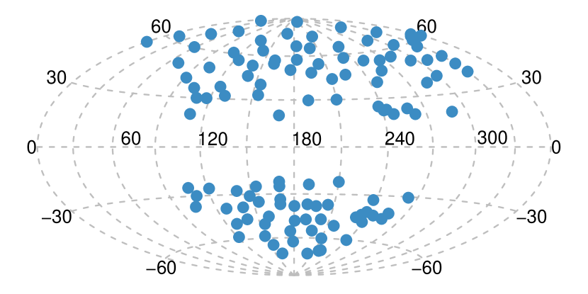
Figure 1.— ECHO-free pure smooth halo sample line-of-sight spatial distribution in Galactic coordinates.

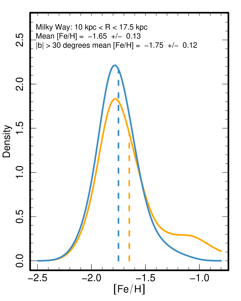
Figure 2.— Density of line-of-sight-averaged metallicity distribution between 10 and 17.5 kpc from the Galactic center in the smooth component of the halo kernel smoothed to 0.1 dex. The orange curve is the distribution for all lines of sight, while the blue curve is the distribution for lines of sight with $|b|>30^{\circ}$. The mean [Fe/H] of each subsample is indicated by the vertical dashed line. Our estimates of the mean metallicity include both random ($\sim\!\!0.01$ dex) and systematic error ($\sim\!\!0.1$ dex). The distribution for the full sample has a heavy tail to high metallicity that is not present at high Galactic latitude. As a result, the mean of the high Galactic latitude sample is systematically more metal poor by about 0.1 dex. This offset is likely related to the metal-rich low-latitude substructure first identified in Monoceros (e.g., Newberg et al., 2002; Belokurov et al., 2006b; Jurić et al., 2008; Ivezić et al., 2008; Schlaufman et al., 2011).

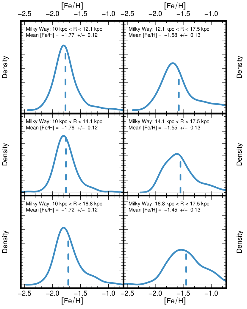
Figure 3.— Density of line-of-sight-averaged metallicity distribution as a function of distance from the Galactic center in the smooth component of the halo kernel smoothed to 0.1 dex. The $y$-axis scale is the same for each panel, and its numerical range is arbitrary such that the area under each curve integrates to 1. We split our tracer sample in two very roughly in distance at three different split points: 12.1, 14.1 and 16.8 kpc. Each row corresponds to the result for a single split-point. In all cases, the nearby part of the sample is in the left column and the distant part of the sample is in the right column. The mean [Fe/H] of each subsample is indicated by the vertical dashed line. Our mean metallicities are in the range $-1.8\lesssim$ [Fe/H] $\lesssim-1.5$. We give the average [Fe/H] and uncertainties in Table 3. We observe no significant metallicity gradient in our sample, though there may be a hint of a positive metallicity gradient at large radius.

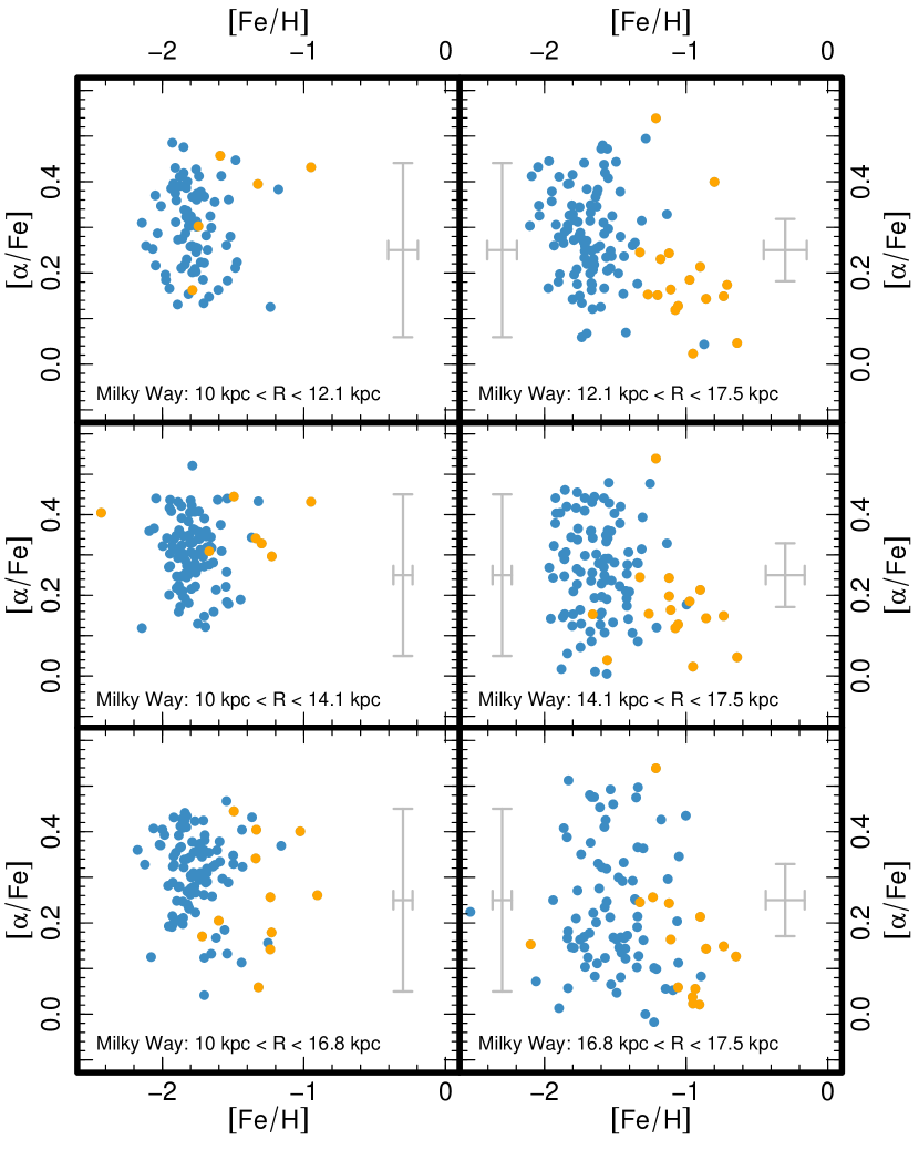
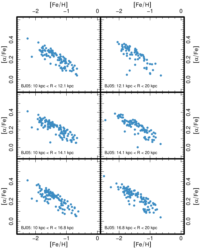
Figure 4.— Line of sight averaged abundance distribution as a function of distance from the Galactic center in the smooth component of the halo in the [Fe/H]–[$\alpha$/Fe] plane. We split our tracer sample in half very roughly in distance at three different split points: 12.1, 14.1 and 16.8 kpc. Each row corresponds to the result for a single split-point. In all cases, the nearby half of the sample is in the left column and the distant half of the sample is in the right column. Left: from Tables 1 and 2, the result for our pure smooth halo MPMSTO population. The typical precision of our measurement is given by the gray error bars. Our precision is a function of metallicity, so if there are two sets of error bars present, the left bars apply for [Fe/H] $\lesssim-1.0$ while the right bars apply for [Fe/H] $\gtrsim-1.0$. We plot in blue lines of sight with $|b|>30^{\circ}$ and in orange lines of sight with $|b|\leq 30^{\circ}$. The smooth halo is dominated by the familiar $-1.8\lesssim$ [Fe/H] $\lesssim-1.5$ and [$\alpha$/Fe]-enhanced population, though at larger distances and low Galactic latitude the pure smooth halo also has a dSph-like component with $\mathrm{[Fe/H]}\approx-1.0$ and [$\alpha$/Fe] $\approx 0.1$. The feature at low Galactic latitude is likely related to the low-latitude substructure first identified in Monoceros (e.g., Newberg et al., 2002; Belokurov et al., 2006b; Jurić et al., 2008; Ivezić et al., 2008; Schlaufman et al., 2011). Right: the equivalent luminosity-weighted average abundance distribution that results from a SEGUE-like observation of halo 10 from Bullock & Johnston (2005). The result is similar for all 11 halos presented in that paper. We discuss the significance of the observed differences between our observations of the Milky Way and of the Bullock & Johnston (2005) models in Section 3.2.

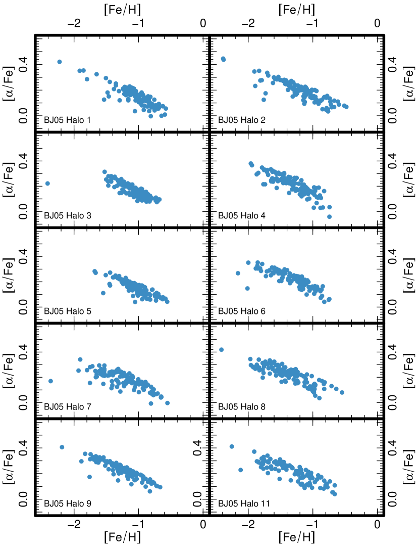
Figure 5.— Line of sight averaged abundance distribution in the [Fe/H]–[$\alpha$/Fe] plane for the other 10 halos from Bullock & Johnston (2005). We include only those star particles with $|z|>4$ kpc that are more than 10 kpc but less than 20 kpc from the center of the halo.

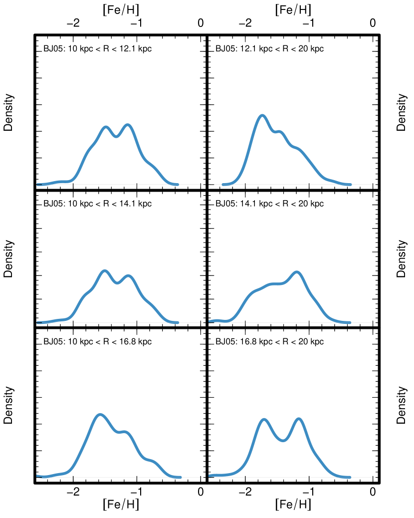
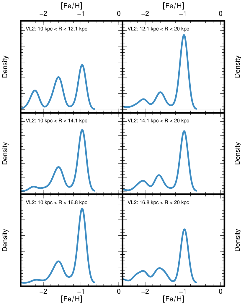
Figure 6.— Density of line-of-sight-averaged metallicity distribution as a function of distance from the center of the halo kernel smoothed to 0.1 dex. Left: halo 10 from Bullock & Johnston (2005). Right: the Via Lactea 2 halo (e.g., Diemand et al., 2008; Madau et al., 2008; Zemp et al., 2009). Dark matter particles in the Via Lactea 2 halo were tagged as star particles with metallicities determined by a simple satellite instantaneous enrichment at accretion model described in Rashkov et al. (2011). The strongly peaked metallicity distribution of the Via Lactea 2 halo is the result of the accretion of two massive satellites with [Fe/H] $\approx-1.0$ at high redshift. Neither dark matter only $N$-body simulation is a good match for our observations of the metallicity of the smooth halo, indicating the importance of gas and in situ star formation in the origin of the smooth halo within 17.5 kpc of the Galactic center.

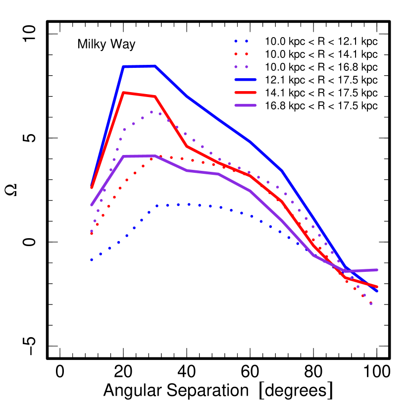
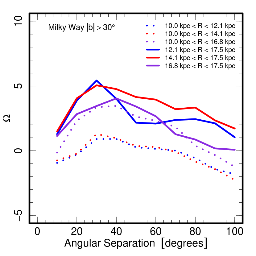
Figure 7.— Quantification of spatial autocorrelation in [Fe/H] in the Galaxy’s pure smooth halo MPMSTO population as a function of Galactocentric distance and angular scale. Positive values of the statistic $\Omega$ indicate spatial autocorrelation. Left: the result for all lines of sight. Right: the result for lines of sight with $|b|>30^{\circ}$. Ignoring the low-latitude substructure and looking only at high Galactic latitude, there is no spatial autocorrelation in [Fe/H] interior to 14.1 kpc. Beyond 14.1 kpc however, there is significant spatial autocorrelation in [Fe/H] with characteristic angular scale between 20^∘ and 30^∘. At 14 kpc – the median Galactocentric distance of the MPMSTO stars in our sample – that corresponds to a physical scale of approximately 5 kpc. This observation suggests that the relative contribution of disrupted satellite galaxies to the stellar population of the smooth halo increases with distance, becoming comparable to the classical smooth halo component at about 15 kpc.

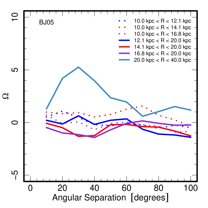
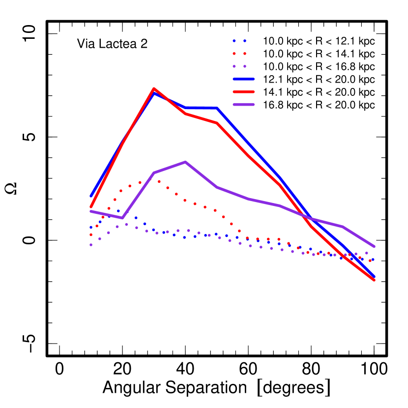
Figure 8.— Quantification of spatial autocorrelation in [Fe/H] in simulations of Milky Way analog formation. Left: halo 10 from Bullock & Johnston (2005). Right: the Via Lactea 2 halo. There is no significant spatial autocorrelation in [Fe/H] within 20 kpc of the center of halo 10 from Bullock & Johnston (2005). There does appear to be significant spatial autocorrelation in [Fe/H] further from the center of the halo, where the Bullock & Johnston (2005) simulations likely model halo formation more accurately. On the other hand, there is significant spatial autocorrelation in [Fe/H] within 20 kpc of the center of the Via Lactea 2 halo. The appearance of significant spatial autocorrelation in [Fe/H] with 20 kpc of the halo center and the angular scale of that spatial autocorrelation in the Via Lactea 2 halo are very similar to the same quantities measured in the halo of the Milky Way. The rapid drop-off in the significance of spatial autocorrelation in [Fe/H] at large angular scale in the Via Lactea 2 halo may indicate that there is less large-scale diffuse substructure in the Via Lactea 2 halo than in the Milky Way. The extra large-scale substructure in the Milky Way may be related to the ongoing merger with the Sagittarius dwarf galaxy.

Table 1Spatial and Radial Distribution of [Fe/H] in the Smooth Component of the Halo

RA	Dec	l	b	bplate	fplate	[Fe/H]in	err	[Fe/H]out	err	[Fe/H]in	err	[Fe/H]out	err	[Fe/H]in	err	[Fe/H]out	err
(deg)	(deg)	(deg)	(deg)
207.22	18.62	3.16	74.29	2905	2930	-2.05	0.14	-1.72	0.20	-1.95	0.15	-1.54	0.09	-1.92	0.16	-1.18	0.13
229.44	7.18	9.84	50.00	2724	2739	-1.76	0.13	-1.97	0.15	-1.90	0.15	$\cdots$	$\cdots$	-1.83	0.16	$\cdots$	$\cdots$
243.77	16.67	31.37	41.94	2177	2188	-1.48	0.10	-1.59	0.17	-1.54	0.09	$\cdots$	$\cdots$	-1.55	0.08	$\cdots$	$\cdots$
238.51	26.52	42.88	49.49	2459	2474	-2.03	0.16	-1.56	0.10	-2.06	0.16	-1.21	0.13	-1.85	0.18	$\cdots$	$\cdots$
253.12	23.95	43.95	36.06	2180	2191	-1.84	0.14	-1.49	0.10	-1.69	0.11	$\cdots$	$\cdots$	-1.69	0.11	$\cdots$	$\cdots$
320.56	-7.18	44.84	-36.65	2305	2320	-1.54	0.09	-1.60	0.20	-1.55	0.09	$\cdots$	$\cdots$	-1.44	0.10	$\cdots$	$\cdots$
311.00	0.00	46.64	-24.82	1908	1909	-1.59	0.17	-0.71	0.08	-1.49	0.10	$\cdots$	$\cdots$	-1.49	0.10	$\cdots$	$\cdots$
261.18	27.01	50.00	30.00	2182	2193	-1.87	0.14	-0.87	0.14	-1.58	0.14	$\cdots$	$\cdots$	-1.58	0.13	$\cdots$	$\cdots$
271.61	23.67	50.00	20.00	2184	2195	-0.95	0.15	$\cdots$	$\cdots$	-0.95	0.15	$\cdots$	$\cdots$	-1.03	0.15	$\cdots$	$\cdots$
317.00	0.00	50.11	-29.97	1918	1919	-1.33	0.12	$\cdots$	$\cdots$	-1.34	0.11	$\cdots$	$\cdots$	-1.34	0.11	$\cdots$	$\cdots$
226.36	32.20	51.02	60.57	2910	2935	-1.85	0.15	-1.60	0.19	-1.81	0.16	-1.55	0.09	-1.84	0.17	$\cdots$	$\cdots$
263.11	33.16	57.36	30.08	2253	2262	-2.14	0.17	-1.56	0.10	-2.09	0.16	-1.86	0.14	-2.17	0.17	$\cdots$	$\cdots$
319.01	10.54	61.22	-25.64	1890	1891	-1.79	0.13	-0.80	0.13	-1.67	0.10	-1.56	0.10	-1.60	0.20	$\cdots$	$\cdots$
344.72	-9.39	61.32	-58.07	1910	1911	-1.71	0.20	-1.44	0.09	-1.81	0.18	-1.71	0.13	-1.65	0.15	$\cdots$	$\cdots$
254.92	39.65	63.60	37.73	2181	2192	-1.18	0.10	-1.66	0.12	-1.32	0.09	-1.41	0.11	-1.37	0.09	$\cdots$	$\cdots$
231.38	39.43	63.98	55.84	2911	2936	-1.53	0.08	-1.74	0.13	-1.55	0.08	-1.64	0.20	-1.50	0.08	-1.29	0.12
212.81	36.58	67.14	70.65	2906	2931	-1.91	0.16	-2.04	0.15	-1.92	0.16	-1.86	0.16	-1.96	0.15	-1.71	0.13
332.78	6.36	67.76	-38.78	2308	2323	-1.63	0.21	-1.70	0.13	-1.61	0.16	-1.80	0.13	-1.61	0.17	-2.52	0.19
341.00	0.00	69.20	-49.10	1900	1901	-1.86	0.18	-1.29	0.12	-1.86	0.18	-1.25	0.12	-2.01	0.16	$\cdots$	$\cdots$
263.44	44.15	70.00	32.00	2799	2820	-2.05	0.16	-1.55	0.08	-1.95	0.17	-1.56	0.11	-1.93	0.17	-1.57	0.14
332.50	21.47	80.06	-27.66	2251	2260	-1.75	0.13	-1.20	0.10	-1.23	0.10	-1.66	0.14	-1.34	0.09	-2.10	0.16
344.84	7.05	80.43	-46.37	2310	2325	-1.79	0.19	-1.58	0.12	-1.77	0.18	-1.00	0.16	-1.74	0.19	-1.23	0.13
340.25	13.68	81.04	-38.36	1892	1893	-2.11	0.14	-1.90	0.16	-2.14	0.13	-1.65	0.18	-2.08	0.13	$\cdots$	$\cdots$
231.76	49.88	81.08	52.66	2449	2464	-1.83	0.17	-1.46	0.08	-1.83	0.18	-1.46	0.08	-1.80	0.18	-1.61	0.21
242.51	52.37	81.35	45.48	2176	2187	-1.83	0.18	-1.63	0.17	-1.87	0.17	-1.67	0.10	-1.90	0.16	-1.75	0.13
217.15	45.26	82.47	63.49	2907	2932	-1.87	0.17	-2.09	0.14	-1.93	0.16	-1.84	0.17	-2.06	0.13	-1.83	0.14
340.97	23.07	88.35	-31.10	2252	2261	-1.48	0.09	-1.58	0.12	-1.69	0.15	-1.42	0.09	-1.50	0.07	-1.36	0.11
356.00	0.00	89.32	-58.40	1902	1903	-1.73	0.19	-1.63	0.22	-1.80	0.18	-1.42	0.10	-1.79	0.18	-1.21	0.13
247.15	62.85	94.00	40.00	2550	2560	-1.79	0.18	-1.58	0.11	-1.85	0.17	-1.47	0.09	-1.92	0.16	-1.60	0.18
262.57	64.37	94.00	33.00	2551	2561	-1.58	0.14	-1.57	0.10	-1.37	0.08	-1.51	0.07	-1.44	0.08	-1.68	0.11
354.52	8.71	94.00	-50.00	2622	2628	-1.75	0.18	-1.61	0.18	-1.79	0.18	-1.76	0.13	-1.83	0.18	$\cdots$	$\cdots$
347.53	22.12	94.00	-35.00	2623	2629	-1.77	0.16	-1.34	0.10	-1.54	0.07	-1.60	0.19	-1.62	0.18	-1.62	0.24
1.02	-4.82	94.00	-65.00	2624	2630	-1.81	0.18	-1.79	0.18	-1.97	0.15	-1.67	0.10	-2.00	0.14	-1.53	0.09
342.14	30.88	94.00	-25.00	2621	2627	$\cdots$	$\cdots$	-1.18	0.13	-1.30	0.12	-1.12	0.14	-1.24	0.13	-0.94	0.15
355.69	14.81	99.18	-44.87	1894	1895	-1.95	0.16	-1.74	0.18	-2.00	0.15	-1.75	0.13	-1.93	0.16	$\cdots$	$\cdots$
217.73	58.24	100.60	54.36	2539	2547	-1.68	0.14	-1.67	0.09	-1.81	0.18	-1.88	0.14	-1.87	0.17	-1.94	0.15
214.83	56.35	100.68	56.81	2447	2462	-1.84	0.17	-1.97	0.15	-1.74	0.19	-1.84	0.17	-1.81	0.18	-1.84	0.16
6.02	-10.00	100.99	-71.69	1912	1913	-1.70	0.19	-1.56	0.08	-1.76	0.19	-1.34	0.10	-1.86	0.17	-1.46	0.10
197.96	39.27	104.92	77.13	2900	2925	-1.91	0.16	-2.10	0.13	-2.04	0.14	-1.96	0.17	-1.98	0.15	-1.68	0.11
1.25	24.95	109.77	-36.73	2801	2822	-1.52	0.09	-1.75	0.18	-1.70	0.18	-1.66	0.11	-1.70	0.19	-1.45	0.10
358.26	36.40	110.00	-25.00	1880	1881	$\cdots$	$\cdots$	-0.64	0.07	$\cdots$	$\cdots$	-0.64	0.07	-1.72	0.13	-0.65	0.08
357.30	39.30	110.00	-22.00	1882	1883	$\cdots$	$\cdots$	-1.06	0.15	$\cdots$	$\cdots$	-1.06	0.15	-1.32	0.12	-0.96	0.15
311.16	76.18	110.00	20.00	2179	2190	$\cdots$	$\cdots$	-0.98	0.16	$\cdots$	$\cdots$	-0.98	0.16	-0.90	0.14	-0.91	0.14
0.64	28.14	110.00	-33.50	2803	2824	$\cdots$	$\cdots$	-1.64	0.16	-1.75	0.14	-1.31	0.09	-1.60	0.13	-1.48	0.09
9.03	7.48	116.28	-55.19	2312	2327	-1.83	0.17	-1.70	0.19	-1.85	0.17	-1.81	0.17	-1.88	0.17	-1.56	0.11
202.79	66.49	116.77	50.16	2445	2460	-1.73	0.19	-1.71	0.20	-1.75	0.19	-1.93	0.17	-1.73	0.19	-1.83	0.16
11.00	0.00	118.86	-62.81	1904	1905	-1.94	0.16	-1.72	0.19	-1.88	0.17	-1.56	0.11	-1.88	0.17	-1.30	0.12
10.51	24.90	120.23	-37.92	2038	2058	-1.67	0.10	-1.84	0.17	-1.87	0.17	-1.68	0.14	-1.85	0.17	-1.72	0.15
11.21	14.92	120.55	-47.93	1896	1897	-1.93	0.17	-1.80	0.19	-1.94	0.16	-1.61	0.18	-2.02	0.14	-1.83	0.14
192.96	59.76	122.84	57.37	2446	2461	-1.74	0.19	-1.75	0.19	-1.80	0.18	-1.66	0.14	-1.86	0.17	-1.78	0.18
192.75	49.74	123.11	67.39	2898	2923	-1.75	0.19	-1.79	0.18	-1.74	0.19	-1.56	0.09	-1.70	0.20	-1.44	0.08
17.86	15.60	130.00	-47.00	2804	2825	-1.75	0.20	-1.77	0.18	-1.67	0.13	-1.62	0.18	-1.71	0.19	-1.34	0.11
19.14	25.74	130.00	-36.79	2040	2060	$\cdots$	$\cdots$	-1.87	0.17	-1.86	0.17	-1.74	0.17	-1.82	0.18	-1.34	0.11
21.15	38.63	130.00	-23.79	2042	2062	$\cdots$	$\cdots$	-1.08	0.13	$\cdots$	$\cdots$	-1.08	0.13	-1.24	0.13	-1.06	0.14
127.07	83.27	130.00	29.71	2541	2549	$\cdots$	$\cdots$	-1.27	0.09	-2.43	0.19	-1.26	0.09	-1.23	0.09	-1.24	0.12
172.12	66.98	134.92	48.17	2858	2873	-1.85	0.17	-1.90	0.16	-1.86	0.17	-1.89	0.16	-1.73	0.19	-1.53	0.07
24.72	23.70	136.73	-37.90	2044	2064	$\cdots$	$\cdots$	-1.70	0.18	-1.59	0.16	-1.66	0.12	-1.64	0.18	-1.46	0.10
21.13	7.21	137.25	-54.74	2314	2329	-1.91	0.16	-1.80	0.18	-1.79	0.18	-1.86	0.18	-1.90	0.16	-1.90	0.14
181.89	49.96	140.22	65.67	2894	2919	-1.76	0.19	-1.75	0.19	-1.79	0.18	-1.80	0.18	-1.80	0.18	-1.57	0.10
18.70	-9.72	141.60	-71.74	2849	2864	-1.91	0.16	-1.67	0.12	-1.90	0.16	-1.52	0.07	-1.86	0.17	-1.35	0.10
26.67	13.98	142.70	-46.76	1898	1899	-1.76	0.13	-1.81	0.18	-1.89	0.17	-1.67	0.13	-1.85	0.17	-1.35	0.11
169.30	59.05	143.49	54.16	2394	2414	-1.80	0.18	-1.90	0.16	-1.84	0.17	-1.77	0.18	-1.92	0.16	-1.46	0.09
32.23	22.52	145.47	-36.94	2046	2066	$\cdots$	$\cdots$	-1.36	0.08	-1.45	0.10	-1.72	0.20	-1.25	0.10	-1.54	0.08
191.46	29.84	147.00	87.02	2457	2472	-1.88	0.17	-1.95	0.15	-1.89	0.16	-1.75	0.20	-1.84	0.17	-1.66	0.15
43.58	34.33	150.00	-22.00	2378	2398	$\cdots$	$\cdots$	-0.95	0.15	$\cdots$	$\cdots$	-0.95	0.15	$\cdots$	$\cdots$	-0.95	0.15
116.19	66.11	150.00	30.00	2939	2944	$\cdots$	$\cdots$	-1.53	0.08	$\cdots$	$\cdots$	-1.53	0.08	-1.56	0.08	-1.30	0.10
26.00	0.00	150.04	-60.08	1906	1907	-1.66	0.14	-2.05	0.14	-1.85	0.17	-1.55	0.07	-1.92	0.16	-1.74	0.14
146.38	62.07	150.92	43.62	2383	2403	$\cdots$	$\cdots$	-1.84	0.17	-1.65	0.15	-1.92	0.16	-1.78	0.19	-1.64	0.19
182.39	39.97	154.34	74.50	2452	2467	-1.80	0.18	-1.77	0.19	-1.95	0.15	-1.80	0.19	-1.88	0.17	-1.43	0.10
33.20	6.62	156.16	-50.93	2306	2321	-1.83	0.16	-1.68	0.15	-1.81	0.18	-1.58	0.12	-1.81	0.18	-1.35	0.10
24.27	-9.45	156.44	-69.30	1914	1915	-1.65	0.15	-1.52	0.07	-1.77	0.19	-1.42	0.08	-1.74	0.19	-1.44	0.09
25.28	-9.39	158.75	-68.73	2850	2865	-1.82	0.18	-1.48	0.08	-1.82	0.18	-1.43	0.08	-1.67	0.14	-1.13	0.13
144.67	52.86	163.48	46.20	2384	2404	$\cdots$	$\cdots$	-1.86	0.17	-1.88	0.17	-1.77	0.19	-1.95	0.15	-1.77	0.19
45.24	5.74	171.39	-44.61	2307	2322	$\cdots$	$\cdots$	-1.67	0.13	-1.79	0.19	-1.34	0.09	-1.76	0.18	-1.38	0.10
158.57	44.34	171.74	57.63	2557	2567	-1.89	0.16	-1.88	0.17	-1.80	0.18	-1.94	0.16	-1.88	0.17	-1.69	0.17
48.25	5.48	174.65	-42.75	2335	2340	$\cdots$	$\cdots$	-1.58	0.11	-1.53	0.08	-1.47	0.08	-1.59	0.14	-1.34	0.11
51.24	5.20	177.71	-40.80	2334	2339	$\cdots$	$\cdots$	-1.44	0.08	-1.79	0.14	-1.58	0.12	-1.54	0.07	-1.14	0.14
57.20	10.31	178.00	-33.00	2679	2697	$\cdots$	$\cdots$	-1.14	0.11	$\cdots$	$\cdots$	-1.14	0.11	-1.16	0.11	-1.05	0.14
113.49	40.89	178.00	25.00	2683	2701	$\cdots$	$\cdots$	-1.11	0.12	$\cdots$	$\cdots$	-1.11	0.12	$\cdots$	$\cdots$	-1.11	0.12
166.97	38.59	178.45	65.54	2856	2871	-1.76	0.19	-1.84	0.17	-1.74	0.19	-1.77	0.18	-1.85	0.17	-1.61	0.17
37.40	-8.47	178.72	-60.22	2047	2067	-1.76	0.19	-1.66	0.14	-1.83	0.18	-1.60	0.13	-1.79	0.18	-1.42	0.09
47.00	0.00	179.01	-47.44	2048	2068	$\cdots$	$\cdots$	-1.67	0.15	-1.69	0.18	-1.55	0.07	-1.72	0.20	-1.58	0.11
111.29	37.62	180.89	22.44	2941	2946	$\cdots$	$\cdots$	-0.90	0.13	$\cdots$	$\cdots$	-0.90	0.13	$\cdots$	$\cdots$	-0.90	0.13
112.51	35.99	182.90	22.87	2053	2073	$\cdots$	$\cdots$	-0.74	0.11	$\cdots$	$\cdots$	-0.74	0.11	$\cdots$	$\cdots$	-0.74	0.11
53.00	0.00	184.53	-42.87	2049	2069	$\cdots$	$\cdots$	-1.62	0.16	-1.76	0.19	-1.55	0.07	-1.69	0.18	-1.34	0.11
134.44	37.13	185.88	40.31	2380	2400	$\cdots$	$\cdots$	-1.68	0.16	-1.77	0.19	-1.67	0.14	-1.70	0.20	-1.86	0.17
110.74	31.44	187.00	20.00	2677	2695	$\cdots$	$\cdots$	-1.21	0.13	$\cdots$	$\cdots$	-1.21	0.13	$\cdots$	$\cdots$	-1.21	0.13
152.52	35.29	189.36	54.80	2387	2407	-1.55	0.08	-1.77	0.19	-1.66	0.14	-1.77	0.18	-1.69	0.17	-1.72	0.17
55.43	-6.41	193.71	-44.60	2050	2070	$\cdots$	$\cdots$	-1.68	0.16	-1.70	0.19	-1.57	0.09	-1.65	0.15	-1.36	0.09
59.42	-5.86	195.91	-40.94	2051	2071	$\cdots$	$\cdots$	-1.70	0.20	-1.64	0.17	-1.75	0.18	-1.70	0.20	-1.79	0.16
144.00	30.05	197.01	47.32	2889	2914	$\cdots$	$\cdots$	-2.04	0.14	-1.94	0.16	-1.87	0.17	-2.12	0.12	-1.47	0.08
118.00	23.20	197.73	23.16	2891	2916	$\cdots$	$\cdots$	-1.12	0.11	$\cdots$	$\cdots$	-1.12	0.11	$\cdots$	$\cdots$	-1.12	0.11
116.00	18.18	201.97	19.54	2054	2074	$\cdots$	$\cdots$	-1.33	0.12	$\cdots$	$\cdots$	-1.33	0.12	$\cdots$	$\cdots$	-1.33	0.12
71.40	-5.68	203.00	-30.48	$\cdots$	2942	$\cdots$	$\cdots$	-1.31	0.09	$\cdots$	$\cdots$	-1.31	0.09	-1.43	0.08	-1.23	0.10
152.38	25.93	205.39	53.92	2386	2406	-1.47	0.08	-1.65	0.15	-1.62	0.15	-1.57	0.10	-1.63	0.16	-1.43	0.08
156.53	17.74	220.87	55.27	2853	2868	-1.92	0.16	-1.67	0.14	-1.89	0.16	-1.61	0.14	-1.83	0.18	-1.49	0.07
141.56	7.30	225.30	37.58	2382	2402	$\cdots$	$\cdots$	-1.92	0.16	-1.72	0.19	-1.92	0.16	-1.86	0.17	-1.84	0.18
169.09	19.29	227.63	66.83	2857	2872	-1.80	0.18	-1.82	0.18	-1.84	0.17	-1.78	0.18	-1.81	0.18	-1.67	0.10
127.96	-4.33	229.00	20.00	2807	2828	$\cdots$	$\cdots$	-0.86	0.13	$\cdots$	$\cdots$	-0.86	0.13	$\cdots$	$\cdots$	-0.86	0.13
156.63	8.82	234.18	51.20	2854	2869	-1.76	0.19	-1.79	0.18	-1.76	0.19	-1.87	0.17	-1.71	0.20	-1.63	0.21
150.00	0.00	239.10	40.72	2852	2867	-1.24	0.10	-1.80	0.18	-1.67	0.14	-1.72	0.19	-1.73	0.19	-1.68	0.11
181.81	19.97	245.85	77.61	2893	2918	-1.90	0.16	-1.74	0.19	-1.87	0.17	-1.86	0.17	-1.87	0.17	-1.64	0.20
168.77	9.61	245.98	61.30	2393	2413	-1.71	0.20	-1.83	0.18	-1.84	0.17	-1.58	0.11	-1.77	0.19	-1.65	0.15
162.00	0.00	250.28	49.82	2389	2409	-1.82	0.18	-1.63	0.16	-1.81	0.18	-1.56	0.09	-1.77	0.19	-1.56	0.09
174.00	0.00	266.09	57.37	2862	2877	-1.76	0.19	-1.93	0.16	-1.77	0.19	-1.85	0.18	-1.77	0.19	-1.81	0.14
180.94	9.98	267.43	69.50	2963	2965	-1.98	0.15	-1.72	0.20	-1.88	0.17	-1.65	0.15	-1.86	0.17	-1.49	0.10
167.16	-16.21	270.00	40.00	2690	2708	-1.70	0.20	-1.89	0.17	-1.73	0.19	-1.60	0.16	-1.53	0.08	-2.06	0.16
169.73	-11.87	270.00	45.00	2859	2874	-1.69	0.17	-1.54	0.07	-1.70	0.20	-1.41	0.08	-1.68	0.17	-1.57	0.13
172.22	-7.52	270.00	50.00	2861	2876	-1.77	0.19	-1.75	0.19	-1.71	0.20	-1.63	0.21	-1.80	0.18	-1.51	0.09
181.00	0.00	278.20	60.57	2892	2917	-2.01	0.14	-1.38	0.08	-1.87	0.17	-1.58	0.12	-1.87	0.17	-1.06	0.15
186.00	0.00	288.15	62.08	2558	2568	-1.60	0.14	-1.56	0.09	-1.64	0.16	-1.38	0.09	-1.75	0.19	-1.09	0.14
189.00	0.00	294.52	62.62	2895	2920	-1.79	0.18	-1.72	0.19	-1.73	0.19	-1.53	0.08	-1.74	0.19	-1.52	0.09
191.00	-2.50	299.18	60.32	2897	2922	-1.89	0.17	-1.55	0.07	-1.90	0.16	-1.41	0.10	-1.82	0.17	-1.00	0.16
191.16	-7.83	300.00	55.00	2689	2707	-1.98	0.16	-1.53	0.07	-1.95	0.15	-1.40	0.10	-1.93	0.16	-0.89	0.14
198.00	0.00	314.09	62.43	2901	2926	-1.84	0.16	-1.47	0.09	-1.71	0.20	-1.51	0.09	-1.71	0.19	$\cdots$	$\cdots$
194.57	19.74	315.26	82.45	2899	2924	-2.07	0.13	-1.65	0.14	-1.94	0.15	-1.35	0.09	-1.93	0.16	-1.06	0.15
205.28	9.39	338.75	68.73	2903	2928	-1.82	0.18	-1.95	0.16	-1.78	0.18	-1.92	0.15	-1.78	0.18	$\cdots$	$\cdots$
217.40	8.47	358.72	60.22	2908	2933	-1.80	0.17	-1.43	0.10	-1.77	0.18	-1.97	0.15	-1.80	0.19	$\cdots$	$\cdots$

Table 2Spatial and Radial Distribution of [$\alpha$/Fe] in the Smooth Component of the Halo

RA	Dec	l	b	bplate	fplate	[$\alpha$/Fe]in	err	[$\alpha$/Fe]out	err	[$\alpha$/Fe]in	err	[$\alpha$/Fe]out	err	[$\alpha$/Fe]in	err	[$\alpha$/Fe]out	err
(deg)	(deg)	(deg)	(deg)
207.22	18.62	3.16	74.29	2905	2930	0.37	0.07	0.44	0.12	0.42	0.06	0.43	0.22	0.43	0.06	0.43	0.22
229.44	7.18	9.84	50.00	2724	2739	0.26	0.16	0.45	0.14	0.22	0.14	$\cdots$	$\cdots$	0.43	0.14	$\cdots$	$\cdots$
243.77	16.67	31.37	41.94	2177	2188	0.45	0.22	0.48	0.17	0.44	0.22	$\cdots$	$\cdots$	0.47	0.21	$\cdots$	$\cdots$
238.51	26.52	42.88	49.49	2459	2474	0.29	0.12	0.21	0.21	0.37	0.11	0.12	0.22	0.21	0.11	$\cdots$	$\cdots$
253.12	23.95	43.95	36.06	2180	2191	0.29	0.16	0.44	0.22	0.32	0.15	$\cdots$	$\cdots$	0.32	0.15	$\cdots$	$\cdots$
320.56	-7.18	44.84	-36.65	2305	2320	0.18	0.22	0.13	0.15	0.22	0.22	$\cdots$	$\cdots$	0.11	0.22	$\cdots$	$\cdots$
311.00	0.00	46.64	-24.82	1908	1909	0.46	0.17	0.17	0.13	0.44	0.22	$\cdots$	$\cdots$	0.44	0.22	$\cdots$	$\cdots$
261.18	27.01	50.00	30.00	2182	2193	0.39	0.15	0.04	0.18	0.31	0.18	$\cdots$	$\cdots$	0.30	0.18	$\cdots$	$\cdots$
271.61	23.67	50.00	20.00	2184	2195	0.43	0.21	$\cdots$	$\cdots$	0.43	0.21	$\cdots$	$\cdots$	0.40	0.22	$\cdots$	$\cdots$
317.00	0.00	50.11	-29.97	1918	1919	0.39	0.22	$\cdots$	$\cdots$	0.34	0.22	$\cdots$	$\cdots$	0.34	0.22	$\cdots$	$\cdots$
226.36	32.20	51.02	60.57	2910	2935	0.42	0.14	0.47	0.16	0.35	0.14	0.48	0.22	0.42	0.13	$\cdots$	$\cdots$
263.11	33.16	57.36	30.08	2253	2262	0.31	0.13	0.47	0.21	0.36	0.13	0.46	0.15	0.36	0.12	$\cdots$	$\cdots$
319.01	10.54	61.22	-25.64	1890	1891	0.16	0.16	0.40	0.16	0.31	0.14	0.04	0.21	0.20	0.15	$\cdots$	$\cdots$
344.72	-9.39	61.32	-58.07	1910	1911	0.19	0.12	0.24	0.21	0.18	0.10	0.30	0.17	0.26	0.08	$\cdots$	$\cdots$
254.92	39.65	63.60	37.73	2181	2192	0.38	0.20	0.12	0.13	0.43	0.18	0.14	0.22	0.43	0.17	$\cdots$	$\cdots$
231.38	39.43	63.98	55.84	2911	2936	0.36	0.14	0.06	0.16	0.26	0.14	0.01	0.13	0.33	0.15	0.00	0.22
212.81	36.58	67.14	70.65	2906	2931	0.37	0.06	0.33	0.09	0.34	0.06	0.25	0.13	0.28	0.06	0.10	0.17
332.78	6.36	67.76	-38.78	2308	2323	0.36	0.11	0.22	0.17	0.44	0.13	0.15	0.16	0.36	0.12	0.22	0.10
341.00	0.00	69.20	-49.10	1900	1901	0.28	0.11	0.49	0.22	0.32	0.10	0.48	0.22	0.37	0.09	$\cdots$	$\cdots$
263.44	44.15	70.00	32.00	2799	2820	0.22	0.10	0.30	0.21	0.20	0.10	0.24	0.21	0.22	0.10	0.23	0.19
332.50	21.47	80.06	-27.66	2251	2260	0.30	0.16	0.15	0.22	0.30	0.21	0.15	0.13	0.40	0.19	0.15	0.13
344.84	7.05	80.43	-46.37	2310	2325	0.37	0.11	0.44	0.17	0.36	0.08	0.18	0.22	0.36	0.08	-0.02	0.22
340.25	13.68	81.04	-38.36	1892	1893	0.26	0.08	0.18	0.12	0.12	0.07	0.44	0.13	0.13	0.08	$\cdots$	$\cdots$
231.76	49.88	81.08	52.66	2449	2464	0.32	0.07	0.28	0.17	0.24	0.07	0.42	0.21	0.30	0.07	0.45	0.15
242.51	52.37	81.35	45.48	2176	2187	0.23	0.07	0.25	0.07	0.25	0.06	0.24	0.11	0.25	0.06	0.16	0.16
217.15	45.26	82.47	63.49	2907	2932	0.21	0.09	0.41	0.08	0.32	0.06	0.42	0.13	0.41	0.06	0.51	0.16
340.97	23.07	88.35	-31.10	2252	2261	0.21	0.22	0.31	0.14	0.36	0.13	0.19	0.21	0.35	0.16	0.25	0.22
356.00	0.00	89.32	-58.40	1902	1903	0.22	0.09	0.38	0.11	0.31	0.08	0.25	0.22	0.38	0.07	0.10	0.22
247.15	62.85	94.00	40.00	2550	2560	0.20	0.07	0.17	0.14	0.20	0.06	0.22	0.21	0.20	0.06	0.32	0.16
262.57	64.37	94.00	33.00	2551	2561	0.41	0.17	0.42	0.13	0.34	0.18	0.40	0.21	0.40	0.17	0.48	0.15
354.52	8.71	94.00	-50.00	2622	2628	0.37	0.09	0.26	0.14	0.42	0.08	0.37	0.16	0.34	0.07	$\cdots$	$\cdots$
347.53	22.12	94.00	-35.00	2623	2629	0.21	0.14	0.18	0.21	0.18	0.20	0.23	0.16	0.17	0.11	0.33	0.13
1.02	-4.82	94.00	-65.00	2624	2630	0.30	0.07	0.27	0.10	0.34	0.06	0.09	0.12	0.40	0.06	0.07	0.22
342.14	30.88	94.00	-25.00	2621	2627	$\cdots$	$\cdots$	0.23	0.22	0.33	0.22	0.20	0.22	0.26	0.22	0.06	0.20
355.69	14.81	99.18	-44.87	1894	1895	0.17	0.10	0.28	0.13	0.32	0.07	0.07	0.16	0.32	0.07	$\cdots$	$\cdots$
217.73	58.24	100.60	54.36	2539	2547	0.25	0.09	0.18	0.12	0.33	0.09	0.02	0.15	0.37	0.08	0.25	0.15
214.83	56.35	100.68	56.81	2447	2462	0.34	0.06	0.17	0.06	0.36	0.07	0.06	0.10	0.23	0.07	0.17	0.14
6.02	-10.00	100.99	-71.69	1912	1913	0.22	0.09	0.21	0.19	0.26	0.07	0.09	0.22	0.20	0.06	0.08	0.22
197.96	39.27	104.92	77.13	2900	2925	0.43	0.06	0.30	0.06	0.44	0.06	0.14	0.10	0.39	0.06	0.18	0.15
1.25	24.95	109.77	-36.73	2801	2822	0.28	0.22	0.15	0.09	0.12	0.11	0.26	0.11	0.04	0.10	0.29	0.22
358.26	36.40	110.00	-25.00	1880	1881	$\cdots$	$\cdots$	0.05	0.10	$\cdots$	$\cdots$	0.05	0.10	0.17	0.17	0.13	0.11
357.30	39.30	110.00	-22.00	1882	1883	$\cdots$	$\cdots$	0.13	0.22	$\cdots$	$\cdots$	0.13	0.22	0.06	0.22	0.04	0.21
311.16	76.18	110.00	20.00	2179	2190	$\cdots$	$\cdots$	0.18	0.22	$\cdots$	$\cdots$	0.18	0.22	0.26	0.19	0.02	0.19
0.64	28.14	110.00	-33.50	2803	2824	$\cdots$	$\cdots$	0.37	0.08	0.13	0.15	0.39	0.20	0.38	0.12	0.30	0.22
9.03	7.48	116.28	-55.19	2312	2327	0.39	0.07	0.27	0.10	0.35	0.06	0.34	0.13	0.39	0.06	0.25	0.21
202.79	66.49	116.77	50.16	2445	2460	0.38	0.07	0.26	0.07	0.34	0.07	0.32	0.10	0.30	0.07	0.18	0.13
11.00	0.00	118.86	-62.81	1904	1905	0.38	0.06	0.25	0.10	0.36	0.06	0.00	0.20	0.36	0.06	0.36	0.22
10.51	24.90	120.23	-37.92	2038	2058	0.15	0.14	0.30	0.06	0.17	0.08	0.11	0.09	0.34	0.06	0.15	0.15
11.21	14.92	120.55	-47.93	1896	1897	0.49	0.10	0.14	0.11	0.44	0.09	0.13	0.14	0.37	0.08	0.06	0.16
192.96	59.76	122.84	57.37	2446	2461	0.41	0.07	0.28	0.07	0.44	0.07	0.34	0.08	0.41	0.06	0.21	0.12
192.75	49.74	123.11	67.39	2898	2923	0.25	0.07	0.32	0.07	0.41	0.07	0.33	0.13	0.38	0.07	0.33	0.21
17.86	15.60	130.00	-47.00	2804	2825	0.37	0.12	0.31	0.09	0.32	0.08	0.28	0.12	0.42	0.08	0.50	0.22
19.14	25.74	130.00	-36.79	2040	2060	$\cdots$	$\cdots$	0.27	0.10	0.21	0.12	0.13	0.14	0.24	0.11	0.13	0.22
21.15	38.63	130.00	-23.79	2042	2062	$\cdots$	$\cdots$	0.12	0.22	$\cdots$	$\cdots$	0.12	0.22	0.14	0.22	0.06	0.22
127.07	83.27	130.00	29.71	2541	2549	$\cdots$	$\cdots$	0.15	0.18	0.40	0.10	0.15	0.18	0.18	0.19	0.26	0.22
172.12	66.98	134.92	48.17	2858	2873	0.48	0.07	0.41	0.06	0.39	0.06	0.40	0.08	0.37	0.07	0.49	0.21
24.72	23.70	136.73	-37.90	2044	2064	$\cdots$	$\cdots$	0.38	0.14	0.37	0.17	0.43	0.14	0.32	0.11	0.13	0.22
21.13	7.21	137.25	-54.74	2314	2329	0.31	0.06	0.42	0.07	0.27	0.07	0.29	0.11	0.35	0.06	0.01	0.15
181.89	49.96	140.22	65.67	2894	2919	0.30	0.07	0.29	0.07	0.33	0.07	0.21	0.08	0.26	0.07	0.43	0.18
18.70	-9.72	141.60	-71.74	2849	2864	0.39	0.06	0.16	0.08	0.35	0.06	0.13	0.18	0.43	0.06	0.19	0.21
26.67	13.98	142.70	-46.76	1898	1899	0.31	0.16	0.35	0.07	0.43	0.06	0.36	0.09	0.32	0.06	0.47	0.22
169.30	59.05	143.49	54.16	2394	2414	0.26	0.07	0.28	0.06	0.25	0.06	0.27	0.08	0.33	0.06	0.17	0.21
32.23	22.52	145.47	-36.94	2046	2066	$\cdots$	$\cdots$	0.27	0.19	0.19	0.22	0.41	0.12	0.16	0.21	0.21	0.21
191.46	29.84	147.00	87.02	2457	2472	0.41	0.06	0.36	0.08	0.31	0.06	0.26	0.12	0.44	0.06	0.22	0.13
43.58	34.33	150.00	-22.00	2378	2398	$\cdots$	$\cdots$	0.02	0.21	$\cdots$	$\cdots$	0.02	0.21	$\cdots$	$\cdots$	0.02	0.21
116.19	66.11	150.00	30.00	2939	2944	$\cdots$	$\cdots$	0.24	0.15	$\cdots$	$\cdots$	0.24	0.15	0.18	0.16	0.16	0.21
26.00	0.00	150.04	-60.08	1906	1907	0.32	0.08	0.43	0.06	0.30	0.06	0.36	0.18	0.35	0.06	0.35	0.16
146.38	62.07	150.92	43.62	2383	2403	$\cdots$	$\cdots$	0.30	0.06	0.32	0.07	0.38	0.07	0.31	0.07	0.20	0.10
182.39	39.97	154.34	74.50	2452	2467	0.32	0.07	0.18	0.07	0.30	0.06	0.12	0.11	0.28	0.06	0.14	0.22
33.20	6.62	156.16	-50.93	2306	2321	0.34	0.14	0.33	0.08	0.25	0.07	0.27	0.16	0.23	0.07	0.10	0.22
24.27	-9.45	156.44	-69.30	1914	1915	0.30	0.07	0.32	0.15	0.28	0.07	0.17	0.20	0.29	0.07	0.17	0.21
25.28	-9.39	158.75	-68.73	2850	2865	0.32	0.07	0.20	0.15	0.38	0.07	0.21	0.17	0.35	0.09	0.30	0.22
144.67	52.86	163.48	46.20	2384	2404	$\cdots$	$\cdots$	0.29	0.06	0.22	0.06	0.34	0.07	0.19	0.06	0.27	0.11
45.24	5.74	171.39	-44.61	2307	2322	$\cdots$	$\cdots$	0.17	0.08	0.30	0.11	0.28	0.20	0.27	0.10	0.29	0.21
158.57	44.34	171.74	57.63	2557	2567	0.27	0.07	0.28	0.06	0.22	0.07	0.24	0.06	0.28	0.06	0.12	0.12
48.25	5.48	174.65	-42.75	2335	2340	$\cdots$	$\cdots$	0.29	0.16	0.18	0.21	0.38	0.21	0.33	0.15	0.21	0.22
51.24	5.20	177.71	-40.80	2334	2339	$\cdots$	$\cdots$	0.15	0.19	0.52	0.16	0.11	0.18	0.13	0.20	0.06	0.22
57.20	10.31	178.00	-33.00	2679	2697	$\cdots$	$\cdots$	0.33	0.22	$\cdots$	$\cdots$	0.33	0.22	0.37	0.22	0.35	0.22
113.49	40.89	178.00	25.00	2683	2701	$\cdots$	$\cdots$	0.16	0.22	$\cdots$	$\cdots$	0.16	0.22	$\cdots$	$\cdots$	0.16	0.22
166.97	38.59	178.45	65.54	2856	2871	0.43	0.07	0.39	0.06	0.34	0.07	0.45	0.08	0.42	0.06	0.28	0.12
37.40	-8.47	178.72	-60.22	2047	2067	0.36	0.07	0.21	0.08	0.27	0.07	0.16	0.11	0.28	0.07	0.17	0.21
47.00	0.00	179.01	-47.44	2048	2068	$\cdots$	$\cdots$	0.35	0.08	0.35	0.07	0.29	0.15	0.34	0.07	0.41	0.17
111.29	37.62	180.89	22.44	2941	2946	$\cdots$	$\cdots$	0.21	0.20	$\cdots$	$\cdots$	0.21	0.20	$\cdots$	$\cdots$	0.21	0.20
112.51	35.99	182.90	22.87	2053	2073	$\cdots$	$\cdots$	0.15	0.14	$\cdots$	$\cdots$	0.15	0.14	$\cdots$	$\cdots$	0.15	0.14
53.00	0.00	184.53	-42.87	2049	2069	$\cdots$	$\cdots$	0.38	0.07	0.26	0.10	0.34	0.19	0.29	0.08	0.37	0.22
134.44	37.13	185.88	40.31	2380	2400	$\cdots$	$\cdots$	0.31	0.08	0.41	0.11	0.36	0.08	0.39	0.07	0.41	0.10
110.74	31.44	187.00	20.00	2677	2695	$\cdots$	$\cdots$	0.54	0.22	$\cdots$	$\cdots$	0.54	0.22	$\cdots$	$\cdots$	0.54	0.22
152.52	35.29	189.36	54.80	2387	2407	0.26	0.14	0.21	0.07	0.34	0.07	0.23	0.10	0.31	0.08	0.17	0.14
55.43	-6.41	193.71	-44.60	2050	2070	$\cdots$	$\cdots$	0.20	0.08	0.15	0.09	0.35	0.13	0.13	0.07	0.25	0.21
59.42	-5.86	195.91	-40.94	2051	2071	$\cdots$	$\cdots$	0.07	0.07	0.16	0.08	0.16	0.09	0.12	0.08	0.15	0.14
144.00	30.05	197.01	47.32	2889	2914	$\cdots$	$\cdots$	0.35	0.06	0.41	0.06	0.30	0.06	0.33	0.06	0.15	0.19
118.00	23.20	197.73	23.16	2891	2916	$\cdots$	$\cdots$	0.24	0.22	$\cdots$	$\cdots$	0.24	0.22	$\cdots$	$\cdots$	0.24	0.22
116.00	18.18	201.97	19.54	2054	2074	$\cdots$	$\cdots$	0.25	0.22	$\cdots$	$\cdots$	0.25	0.22	$\cdots$	$\cdots$	0.25	0.22
71.40	-5.68	203.00	-30.48	$\cdots$	2942	$\cdots$	$\cdots$	0.31	0.18	$\cdots$	$\cdots$	0.31	0.18	0.32	0.19	0.10	0.21
152.38	25.93	205.39	53.92	2386	2406	0.22	0.15	0.22	0.07	0.21	0.06	0.29	0.11	0.33	0.06	0.12	0.19
156.53	17.74	220.87	55.27	2853	2868	0.40	0.06	0.25	0.08	0.29	0.06	0.15	0.07	0.41	0.07	0.16	0.18
141.56	7.30	225.30	37.58	2382	2402	$\cdots$	$\cdots$	0.31	0.06	0.30	0.09	0.40	0.06	0.25	0.06	0.39	0.10
169.09	19.29	227.63	66.83	2857	2872	0.32	0.07	0.39	0.07	0.29	0.06	0.42	0.10	0.34	0.07	0.48	0.11
127.96	-4.33	229.00	20.00	2807	2828	$\cdots$	$\cdots$	0.14	0.18	$\cdots$	$\cdots$	0.14	0.18	$\cdots$	$\cdots$	0.14	0.18
156.63	8.82	234.18	51.20	2854	2869	0.25	0.07	0.20	0.07	0.27	0.07	0.15	0.08	0.26	0.07	0.11	0.11
150.00	0.00	239.10	40.72	2852	2867	0.13	0.21	0.33	0.07	0.28	0.08	0.44	0.09	0.31	0.07	0.38	0.12
181.81	19.97	245.85	77.61	2893	2918	0.36	0.06	0.13	0.11	0.21	0.06	0.15	0.12	0.21	0.06	0.08	0.13
168.77	9.61	245.98	61.30	2393	2413	0.13	0.07	0.33	0.07	0.19	0.06	0.44	0.12	0.28	0.07	0.48	0.11
162.00	0.00	250.28	49.82	2389	2409	0.40	0.07	0.35	0.05	0.41	0.07	0.19	0.13	0.42	0.07	0.32	0.17
174.00	0.00	266.09	57.37	2862	2877	0.20	0.07	0.26	0.09	0.22	0.07	0.31	0.11	0.22	0.07	0.15	0.16
180.94	9.98	267.43	69.50	2963	2965	0.20	0.06	0.23	0.07	0.16	0.06	0.19	0.08	0.21	0.06	0.05	0.22
167.16	-16.21	270.00	40.00	2690	2708	0.37	0.12	0.20	0.10	0.31	0.10	0.20	0.15	0.29	0.14	0.07	0.13
169.73	-11.87	270.00	45.00	2859	2874	0.28	0.09	0.21	0.15	0.39	0.07	0.31	0.21	0.29	0.08	0.12	0.19
172.22	-7.52	270.00	50.00	2861	2876	0.37	0.07	0.34	0.08	0.30	0.07	0.30	0.11	0.28	0.07	0.17	0.22
181.00	0.00	278.20	60.57	2892	2917	0.35	0.07	0.26	0.20	0.42	0.06	0.25	0.17	0.41	0.06	0.11	0.22
186.00	0.00	288.15	62.08	2558	2568	0.16	0.11	0.23	0.15	0.28	0.07	0.11	0.21	0.35	0.07	0.05	0.22
189.00	0.00	294.52	62.62	2895	2920	0.26	0.08	0.27	0.11	0.35	0.07	0.36	0.21	0.37	0.07	0.46	0.22
191.00	-2.50	299.18	60.32	2897	2922	0.13	0.10	0.41	0.19	0.25	0.08	0.28	0.22	0.27	0.08	0.44	0.22
191.16	-7.83	300.00	55.00	2689	2707	0.18	0.09	0.25	0.18	0.27	0.08	0.21	0.22	0.19	0.08	0.08	0.19
198.00	0.00	314.09	62.43	2901	2926	0.22	0.14	0.38	0.21	0.27	0.12	0.28	0.22	0.36	0.11	$\cdots$	$\cdots$
194.57	19.74	315.26	82.45	2899	2924	0.25	0.06	0.23	0.08	0.27	0.06	0.28	0.21	0.29	0.06	0.20	0.22
205.28	9.39	338.75	68.73	2903	2928	0.15	0.11	0.38	0.12	0.36	0.10	0.44	0.15	0.35	0.09	$\cdots$	$\cdots$
217.40	8.47	358.72	60.22	2908	2933	0.30	0.13	0.07	0.22	0.30	0.13	0.27	0.14	0.30	0.12	$\cdots$	$\cdots$

Table 3Mean [Fe/H] in the Smooth Component of the Halo

Volume	Mean [Fe/H]	err	Mean [Fe/H] Above $|b|=30^{\circ}$	err
10.0 kpc $\lesssim d\lesssim$ 12.1 kpc	-1.77	0.12	-1.78	0.12
10.0 kpc $\lesssim d\lesssim$ 14.1 kpc	-1.78	0.12	-1.79	0.11
10.0 kpc $\lesssim d\lesssim$ 16.8 kpc	-1.72	0.12	-1.77	0.12
10.0 kpc $\lesssim d\lesssim$ 17.5 kpc	-1.65	0.13	-1.75	0.12
12.1 kpc $\lesssim d\lesssim$ 17.5 kpc	-1.58	0.13	-1.69	0.12
14.1 kpc $\lesssim d\lesssim$ 17.5 kpc	-1.55	0.13	-1.63	0.12
16.8 kpc $\lesssim d\lesssim$ 17.5 kpc	-1.45	0.13	-1.53	0.13

Table 4Spatial Autocorrelation in [Fe/H] in the Smooth Component of the Halo

Volume	$I$	E$(I)$	Var$(I)$	$p$-value
10.0 kpc $\lesssim d\lesssim$ 12.1 kpc	-0.012	-0.012	0.019	1.0e+00
10.0 kpc $\lesssim d\lesssim$ 14.1 kpc	0.018	-0.010	0.016	8.2e-02
10.0 kpc $\lesssim d\lesssim$ 16.8 kpc	0.049	-0.009	0.015	1.2e-04
12.1 kpc $\lesssim d\lesssim$ 17.5 kpc	0.110	-0.009	0.015	4.4e-16
14.1 kpc $\lesssim d\lesssim$ 17.5 kpc	0.113	-0.009	0.016	3.1e-15
16.8 kpc $\lesssim d\lesssim$ 17.5 kpc	0.077	-0.010	0.018	1.3e-06

Note. — The five columns are: range in distance from the Galactic center, Moran’s $I$ statistic indicating the degree of spatial autocorrelation in the data in Table 1, the expected value of Moran’s $I$ statistic under the null hypothesis that there is no spatial autocorrelation, the variance of the expected value under the null hypothesis, and the probability that the null hypothesis applies to the data in Table 1.

Table 5Spatial Autocorrelation in [Fe/H] Above $|b|=30^{\circ}$ in the Smooth Component of the Halo

Volume	$I$	E$(I)$	Var$(I)$	$p$-value
10.0 kpc $\lesssim d\lesssim$ 12.1 kpc	-0.033	-0.013	0.021	3.5e-01
10.0 kpc $\lesssim d\lesssim$ 14.1 kpc	-0.018	-0.011	0.018	6.7e-01
10.0 kpc $\lesssim d\lesssim$ 16.8 kpc	0.026	-0.010	0.017	3.5e-02
12.1 kpc $\lesssim d\lesssim$ 17.5 kpc	0.070	-0.010	0.018	4.7e-06
14.1 kpc $\lesssim d\lesssim$ 17.5 kpc	0.088	-0.011	0.019	1.1e-07
16.8 kpc $\lesssim d\lesssim$ 17.5 kpc	0.067	-0.012	0.022	2.1e-04

Table 6Spatial Autocorrelation in [Fe/H] in Bullock & Johnston (2005) Halos

Halo	Volume	$I$	E$(I)$	Var$(I)$	$p$-value
1	10.0 kpc $<d<$ 12.1 kpc	0.006	-0.009	0.015	3.3e-01
	10.0 kpc $<d<$ 14.1 kpc	0.001	-0.008	0.014	5.1e-01
	10.0 kpc $<d<$ 16.8 kpc	-0.016	-0.008	0.015	5.9e-01
	12.1 kpc $<d<$ 20.0 kpc	-0.009	-0.008	0.015	9.6e-01
	14.1 kpc $<d<$ 20.0 kpc	0.044	-0.008	0.015	4.3e-04
	16.8 kpc $<d<$ 20.0 kpc	-0.023	-0.038	0.048	7.4e-01
2	10.0 kpc $<d<$ 12.1 kpc	0.011	-0.009	0.016	2.1e-01
	10.0 kpc $<d<$ 14.1 kpc	-0.005	-0.009	0.015	8.3e-01
	10.0 kpc $<d<$ 16.8 kpc	0.008	-0.008	0.015	2.8e-01
	12.1 kpc $<d<$ 20.0 kpc	0.018	-0.008	0.015	7.8e-02
	14.1 kpc $<d<$ 20.0 kpc	0.015	-0.008	0.015	1.1e-01
	16.8 kpc $<d<$ 20.0 kpc	0.009	-0.030	0.059	5.0e-01
3	10.0 kpc $<d<$ 12.1 kpc	-0.016	-0.009	0.014	6.1e-01
	10.0 kpc $<d<$ 14.1 kpc	-0.005	-0.008	0.013	7.8e-01
	10.0 kpc $<d<$ 16.8 kpc	0.002	-0.008	0.014	4.7e-01
	12.1 kpc $<d<$ 20.0 kpc	0.018	-0.008	0.015	7.6e-02
	14.1 kpc $<d<$ 20.0 kpc	0.024	-0.009	0.015	3.3e-02
	16.8 kpc $<d<$ 20.0 kpc	-0.047	-0.037	0.066	8.8e-01
4	10.0 kpc $<d<$ 12.1 kpc	0.018	-0.009	0.016	8.6e-02
	10.0 kpc $<d<$ 14.1 kpc	0.002	-0.008	0.015	4.7e-01
	10.0 kpc $<d<$ 16.8 kpc	0.012	-0.008	0.015	1.7e-01
	12.1 kpc $<d<$ 20.0 kpc	-0.001	-0.008	0.015	6.0e-01
	14.1 kpc $<d<$ 20.0 kpc	0.004	-0.008	0.015	4.0e-01
	16.8 kpc $<d<$ 20.0 kpc	0.264	-0.023	0.037	1.2e-14
5	10.0 kpc $<d<$ 12.1 kpc	0.005	-0.009	0.016	3.9e-01
	10.0 kpc $<d<$ 14.1 kpc	-0.002	-0.009	0.015	6.9e-01
	10.0 kpc $<d<$ 16.8 kpc	-0.005	-0.009	0.015	8.0e-01
	12.1 kpc $<d<$ 20.0 kpc	-0.003	-0.009	0.015	7.0e-01
	14.1 kpc $<d<$ 20.0 kpc	-0.009	-0.009	0.015	9.9e-01
	16.8 kpc $<d<$ 20.0 kpc	-0.024	-0.028	0.050	9.3e-01
6	10.0 kpc $<d<$ 12.1 kpc	0.037	-0.009	0.016	3.9e-03
	10.0 kpc $<d<$ 14.1 kpc	0.025	-0.008	0.015	2.6e-02
	10.0 kpc $<d<$ 16.8 kpc	0.037	-0.008	0.015	2.5e-03
	12.1 kpc $<d<$ 20.0 kpc	0.006	-0.008	0.015	3.3e-01
	14.1 kpc $<d<$ 20.0 kpc	0.000	-0.008	0.014	5.4e-01
	16.8 kpc $<d<$ 20.0 kpc	-0.052	-0.023	0.038	4.5e-01
7	10.0 kpc $<d<$ 12.1 kpc	-0.012	-0.009	0.016	8.8e-01
	10.0 kpc $<d<$ 14.1 kpc	0.021	-0.009	0.015	5.1e-02
	10.0 kpc $<d<$ 16.8 kpc	0.037	-0.008	0.015	2.7e-03
	12.1 kpc $<d<$ 20.0 kpc	0.016	-0.008	0.015	1.0e-01
	14.1 kpc $<d<$ 20.0 kpc	0.000	-0.009	0.015	5.6e-01
	16.8 kpc $<d<$ 20.0 kpc	0.067	-0.036	0.064	1.1e-01
8	10.0 kpc $<d<$ 12.1 kpc	-0.007	-0.009	0.016	9.1e-01
	10.0 kpc $<d<$ 14.1 kpc	-0.015	-0.008	0.015	6.7e-01
	10.0 kpc $<d<$ 16.8 kpc	-0.004	-0.008	0.015	7.5e-01
	12.1 kpc $<d<$ 20.0 kpc	0.022	-0.008	0.015	3.8e-02
	14.1 kpc $<d<$ 20.0 kpc	0.026	-0.008	0.015	1.9e-02
	16.8 kpc $<d<$ 20.0 kpc	0.042	-0.018	0.032	6.5e-02
9	10.0 kpc $<d<$ 12.1 kpc	-0.022	-0.009	0.016	4.2e-01
	10.0 kpc $<d<$ 14.1 kpc	-0.035	-0.008	0.015	7.6e-02
	10.0 kpc $<d<$ 16.8 kpc	-0.006	-0.008	0.015	8.6e-01
	12.1 kpc $<d<$ 20.0 kpc	0.019	-0.008	0.014	5.6e-02
	14.1 kpc $<d<$ 20.0 kpc	0.021	-0.008	0.015	4.5e-02
	16.8 kpc $<d<$ 20.0 kpc	-0.034	-0.029	0.034	8.6e-01
10	10.0 kpc $<d<$ 12.1 kpc	0.002	-0.009	0.016	5.0e-01
	10.0 kpc $<d<$ 14.1 kpc	0.021	-0.008	0.014	4.1e-02
	10.0 kpc $<d<$ 16.8 kpc	-0.002	-0.008	0.014	6.6e-01
	12.1 kpc $<d<$ 20.0 kpc	-0.007	-0.008	0.015	9.5e-01
	14.1 kpc $<d<$ 20.0 kpc	-0.023	-0.008	0.015	3.3e-01
	16.8 kpc $<d<$ 20.0 kpc	-0.055	-0.028	0.037	4.7e-01
11	10.0 kpc $<d<$ 12.1 kpc	0.041	-0.014	0.024	2.2e-02
	10.0 kpc $<d<$ 14.1 kpc	0.036	-0.011	0.019	1.2e-02
	10.0 kpc $<d<$ 16.8 kpc	0.027	-0.009	0.016	2.5e-02
	12.1 kpc $<d<$ 20.0 kpc	0.036	-0.008	0.015	2.6e-03
	14.1 kpc $<d<$ 20.0 kpc	0.057	-0.009	0.016	2.4e-05
	16.8 kpc $<d<$ 20.0 kpc	0.049	-0.010	0.018	9.7e-04

Table 7Spatial Autocorrelation in [Fe/H] in Via Lactea 2

Volume	$I$	E$(I)$	Var$(I)$	$p$-value
10.0 kpc $<d<$ 12.1 kpc	0.025	-0.019	0.033	1.8e-01
10.0 kpc $<d<$ 14.1 kpc	0.067	-0.015	0.024	7.5e-04
10.0 kpc $<d<$ 16.8 kpc	0.003	-0.012	0.020	4.4e-01
12.1 kpc $<d<$ 20.0 kpc	0.079	-0.011	0.019	1.3e-06
14.1 kpc $<d<$ 20.0 kpc	0.078	-0.012	0.020	8.9e-06
16.8 kpc $<d<$ 20.0 kpc	0.043	-0.015	0.025	1.9e-02

References

- Abazajian et al. (2009) Abazajian, K. N., Adelman-McCarthy, J. K., Agüeros, M. A., et al. 2009, ApJS, 182, 543
- Allende Prieto et al. (2006) Allende Prieto, C., Beers, T. C., Wilhelm, R., et al. 2006, ApJ, 636, 804
- Allende Prieto et al. (2008) Allende Prieto, C., Sivarani, T., Beers, T. C., et al. 2008, AJ, 136, 2070
- An et al. (2009) An, D., Johnson, J. A., Beers, T. C., et al. 2009, ApJ, 707, L64
- An et al. (2008) An, D., Johnson, J. A., Clem, J. L., et al. 2008, ApJS, 179, 326
- Beers et al. (2012) Beers, T. C., Carollo, D., Ivezić, Ž., et al. 2012, ApJ, 746, 34
- Bell et al. (2008) Bell, E. F., Zucker, D. B., Belokurov, V., et al. 2008, ApJ, 680, 295
- Belokurov et al. (2006a) Belokurov, V., Evans, N. W., Irwin, M. J., Hewett, P. C., & Wilkinson, M. I. 2006a, ApJ, 637, L29
- Belokurov et al. (2006b) Belokurov, V., Zucker, D. B., Evans, N. W., et al. 2006, ApJ, 642, L137
- Belokurov et al. (2007) Belokurov, V., Evans, N. W., Irwin, M. J., et al. 2007, ApJ, 658, 337
- Bensby et al. (2003) Bensby, T., Feltzing, S., & Lundström, I. 2003, A&A, 410, 527
- Bland-Hawthorn et al. (2010) Bland-Hawthorn, J., Krumholz, M. R., & Freeman, K. 2010, ApJ, 713, 166
- Bubar & King (2010) Bubar, E. J., & King, J. R. 2010, AJ, 140, 293
- Bullock & Johnston (2005) Bullock, J. S., & Johnston, K. V. 2005, ApJ, 635, 931
- Carollo et al. (2007) Carollo, D., Beers, T. C., Lee, Y. S., et al. 2007, Nature, 450, 1020
- Carollo et al. (2010) Carollo, D., Beers, T. C., Chiba, M., et al. 2010, ApJ, 712, 692
- Carollo et al. (2012) Carollo, D., Beers, T. C., Bovy, J., et al. 2012, ApJ, 744, 195
- Chiba & Beers (2000) Chiba, M., & Beers, T. C. 2000, AJ, 119, 2843
- Chiba & Yoshii (1998) Chiba, M., & Yoshii, Y. 1998, AJ, 115, 168
- Cliff & Ord (1981) Cliff, A. D., & Ord, K. K. 1981, Spatial Processes: Models and Applications (London: Pion)
- Cooper et al. (2010) Cooper, A. P., Cole, S., Frenk, C. S., et al. 2010, MNRAS, 406, 744
- de Jong et al. (2010) de Jong, J. T. A., Yanny, B., Rix, H.-W., et al. 2010, ApJ, 714, 663
- De Silva et al. (2007a) De Silva, G. M., Freeman, K. C., Asplund, M., et al. 2007, AJ, 133, 1161
- De Silva et al. (2007b) De Silva, G. M., Freeman, K. C., Bland-Hawthorn, J., Asplund, M., & Bessell, M. S. 2007, AJ, 133, 694
- De Silva et al. (2006) De Silva, G. M., Sneden, C., Paulson, D. B., et al. 2006, AJ, 131, 455
- Diemand et al. (2008) Diemand, J., Kuhlen, M., Madau, P., et al. 2008, Nature, 454, 735
- Duffau et al. (2006) Duffau, S., Zinn, R., Vivas, A. K., et al. 2006, ApJ, 636, L97
- Edvardsson et al. (1993) Edvardsson, B., Andersen, J., Gustafsson, B., et al. 1993, A&A, 275, 101
- Font et al. (2006a) Font, A. S., Johnston, K. V., Bullock, J. S., & Robertson, B. E. 2006a, ApJ, 638, 585
- Font et al. (2006b) Font, A. S., Johnston, K. V., Bullock, J. S., & Robertson, B. E. 2006b, ApJ, 646, 886
- Font et al. (2011) Font, A. S., McCarthy, I. G., Crain, R. A., et al. 2011, MNRAS, 1162
- Fukugita et al. (1996) Fukugita, M., Ichikawa, T., Gunn, J. E., et al. 1996, AJ, 111, 1748
- Fulbright (2000) Fulbright, J. P. 2000, AJ, 120, 1841
- Gilmore et al. (2002) Gilmore, G., Wyse, R. F. G., & Norris, J. E. 2002, ApJ, 574, L39
- Grillmair (2009) Grillmair, C. J. 2009, ApJ, 693, 1118
- Grillmair & Dionatos (2006) Grillmair, C. J., & Dionatos, O. 2006, ApJ, 643, L17
- Grillmair & Johnson (2006) Grillmair, C. J., & Johnson, R. 2006, ApJ, 639, L17
- Gunn et al. (1998) Gunn, J. E., Carr, M., Rockosi, C., et al. 1998, AJ, 116, 3040
- Gunn et al. (2006) Gunn, J. E., Siegmund, W. A., Mannery, E. J., et al. 2006, AJ, 131, 2332
- Hanson et al. (1998) Hanson, R. B., Sneden, C., Kraft, R. P., & Fulbright, J. 1998, AJ, 116, 1286
- Helmi (2008) Helmi, A. 2008, A&A Rev., 15, 145
- Helmi et al. (2011) Helmi, A., Cooper, A. P., White, S. D. M., et al. 2011, ApJ, 733, L7
- Helmi et al. (1999) Helmi, A., White, S. D. M., de Zeeuw, P. T., & Zhao, H. 1999, Nature, 402, 53
- Hogg et al. (2001) Hogg, D. W., Finkbeiner, D. P., Schlegel, D. J., & Gunn, J. E. 2001, AJ, 122, 2129
- Ivezić et al. (2000) Ivezić, Ž., Goldston, J., Finlator, K., et al. 2000, AJ, 120, 963
- Ivezić et al. (2004) Ivezić, Ž., Lupton, R. H., Schlegel, D., et al. 2004, Astronomische Nachrichten, 325, 583
- Ivezić et al. (2008) Ivezić, Ž., Sesar, B., Jurić, M., et al. 2008, ApJ, 684, 287
- Jurić et al. (2008) Jurić, M., Ivezić, Ž., Brooks, A., et al. 2008, ApJ, 673, 864
- Kazantzidis et al. (2008) Kazantzidis, S., Bullock, J. S., Zentner, A. R., Kravtsov, A. V., & Moustakas, L. A. 2008, ApJ, 688, 254
- Kazantzidis et al. (2009) Kazantzidis, S., Zentner, A. R., Kravtsov, A. V., Bullock, J. S., & Debattista, V. P. 2009, ApJ, 700, 1896
- Kepley et al. (2007) Kepley, A. A., Morrison, H. L., Helmi, A., et al. 2007, AJ, 134, 1579
- Kirby et al. (2011a) Kirby, E. N., Cohen, J. G., Smith, G. H., et al. 2011, ApJ, 727, 79
- Kirby et al. (2011b) Kirby, E. N., Lanfranchi, G. A., Simon, J. D., Cohen, J. G., & Guhathakurta, P. 2011b, ApJ, 727, 78
- Kirby et al. (2010) Kirby, E. N., Guhathakurta, P., Simon, J. D., et al. 2010, ApJS, 191, 352
- Klement et al. (2008) Klement, R., Fuchs, B., & Rix, H.-W. 2008, ApJ, 685, 261
- Klement et al. (2009) Klement, R., Rix, H.-W., Flynn, C., et al. 2009, ApJ, 698, 865
- Lee et al. (2011) Lee, Y. S., Beers, T. C., Allende Prieto, C., et al. 2011, AJ, 141, 90
- Lee et al. (2008a) Lee, Y. S., Beers, T. C., Sivarani, T., et al. 2008, AJ, 136, 2022
- Lee et al. (2008b) Lee, Y. S., Beers, T. C., Sivarani, T., et al. 2008, AJ, 136, 2050
- Maciejewski et al. (2011) Maciejewski, M., Vogelsberger, M., White, S. D. M., & Springel, V. 2011, MNRAS, 415, 2475
- Madau et al. (2008) Madau, P., Kuhlen, M., Diemand, J., et al. 2008, ApJ, 689, L41
- Majewski et al. (1996) Majewski, S. R., Munn, J. A., & Hawley, S. L. 1996, ApJ, 459, L73
- Majewski et al. (2003) Majewski, S. R., Skrutskie, M. F., Weinberg, M. D., & Ostheimer, J. C. 2003, ApJ, 599, 1082
- Mateo (1998) Mateo, M. L. 1998, ARA&A, 36, 435
- McCarthy et al. (2011) McCarthy, I. G., Font, A. S., Crain, R. A., et al. 2011, arXiv:1111.1747
- McWilliam et al. (1995) McWilliam, A., Preston, G. W., Sneden, C., & Searle, L. 1995, AJ, 109, 2757
- Moran (1950) Moran, P. A. P. 1950, Biometrika, 37, 17
- Newberg et al. (2002) Newberg, H. J., Yanny, B., Rockosi, C., et al. 2002, ApJ, 569, 245
- Nissen & Schuster (1997) Nissen, P. E., & Schuster, W. J. 1997, A&A, 326, 751
- Odenkirchen et al. (2001) Odenkirchen, M., Grebel, E. K., Rockosi, C. M., et al. 2001, ApJ, 548, L165
- Padmanabhan et al. (2008) Padmanabhan, N., Schlegel, D. J., Finkbeiner, D. P., et al. 2008, ApJ, 674, 1217
- Pier et al. (2003) Pier, J. R., Munn, J. A., Hindsley, R. B., et al. 2003, AJ, 125, 1559
- Pompéia et al. (2011) Pompéia, L., Masseron, T., Famaey, B., et al. 2011, MNRAS, 415, 1138
- Prochaska et al. (2000) Prochaska, J. X., Naumov, S. O., Carney, B. W., McWilliam, A., & Wolfe, A. M. 2000, AJ, 120, 2513
- Purcell et al. (2010) Purcell, C. W., Bullock, J. S., & Kazantzidis, S. 2010, MNRAS, 404, 1711
- Purcell et al. (2011) Purcell, C. W., Bullock, J. S., Tollerud, E. J., Rocha, M., & Chakrabarti, S. 2011, Nature, 477, 301
- Rashkov et al. (2011) Rashkov, V., Madau, P., Kuhlen, M., & Diemand, J. 2011, ApJ, 745, 142
- Reddy et al. (2003) Reddy, B. E., Tomkin, J., Lambert, D. L., & Allende Prieto, C. 2003, MNRAS, 340, 304
- Robertson et al. (2005) Robertson, B., Bullock, J. S., Font, A. S., Johnston, K. V., & Hernquist, L. 2005, ApJ, 632, 872
- Rocha-Pinto et al. (2004) Rocha-Pinto, H. J., Majewski, S. R., Skrutskie, M. F., Crane, J. D., & Patterson, R. J. 2004, ApJ, 615, 732
- Rockosi et al. (2002) Rockosi, C. M., Odenkirchen, M., Grebel, E. K., et al. 2002, AJ, 124, 349
- Ryan & Norris (1991a) Ryan, S. G., & Norris, J. E. 1991a, AJ, 101, 1835
- Ryan & Norris (1991b) Ryan, S. G., & Norris, J. E. 1991b, AJ, 101, 1865
- Schlaufman et al. (2009) Schlaufman, K. C., Rockosi, C. M., Allende Prieto, C., et al. 2009, ApJ, 703, 2177
- Schlaufman et al. (2011) Schlaufman, K. C., Rockosi, C. M., Lee, Y. S., Beers, T. C., & Allende Prieto, C. 2011, ApJ, 734, 49
- Seabroke et al. (2008) Seabroke, G. M., Gilmore, G., Siebert, A., et al. 2008, MNRAS, 384, 11
- Sesar et al. (2007) Sesar, B., Ivezić, Ž., Lupton, R. H., et al. 2007, AJ, 134, 2236
- Sesar et al. (2011) Sesar, B., Jurić, M., & Ivezić, Ž. 2011, ApJ, 731, 4
- Smith et al. (2002) Smith, J. A., Tucker, D. L., Kent, S., et al. 2002, AJ, 123, 2121
- Smith et al. (2009) Smith, M. C., Evans, N. W., Belokurov, V., et al. 2009, MNRAS, 399, 1223
- Smolinski et al. (2011) Smolinski, J. P., Lee, Y. S., Beers, T. C., et al. 2011, AJ, 141, 89
- Starkenburg et al. (2009) Starkenburg, E., Helmi, A., Morrison, H. L., et al. 2009, ApJ, 698, 567
- Stephens & Boesgaard (2002) Stephens, A., & Boesgaard, A. M. 2002, AJ, 123, 1647
- Tissera et al. (2012) Tissera, P. B., White, S. D. M., & Scannapieco, C. 2012, MNRAS, 420, 255
- Totten & Irwin (1998) Totten, E. J., & Irwin, M. J. 1998, MNRAS, 294, 1
- Totten et al. (2000) Totten, E. J., Irwin, M. J., & Whitelock, P. A. 2000, MNRAS, 314, 630
- Tucker et al. (2006) Tucker, D. L., Kent, S., Richmond, M. W., et al. 2006, Astronomische Nachrichten, 327, 821
- Venn et al. (2004) Venn, K. A., Irwin, M., Shetrone, M. D., et al. 2004, AJ, 128, 1177
- Vivas & Zinn (2006) Vivas, A. K., & Zinn, R. 2006, AJ, 132, 714
- Vivas et al. (2001) Vivas, A. K., Zinn, R., Andrews, P., et al. 2001, ApJ, 554, L33
- Waller & Gotway (2004) Waller, L. A., & Gotway, C. A. 2004, Applied Spatial Statistics for Public Health Data (Hoboken, NY: John Wiley & Sons, Inc.)
- Watkins et al. (2009) Watkins, L. L., Evans, N. W., Belokurov, V., et al. 2009, MNRAS, 398, 1757
- Xue et al. (2011) Xue, X.-X., Rix, H.-W., Yanny, B., et al. 2011, ApJ, 738, 79
- Yanny et al. (2003) Yanny, B., Newberg, H. J., Grebel, E. K., et al. 2003, ApJ, 588, 824
- Yanny et al. (2000) Yanny, B., Newberg, H. J., Kent, S., et al. 2000, ApJ, 540, 825
- Yanny et al. (2009) Yanny, B., Rockosi, C., Newberg, H. J., et al. 2009, AJ, 137, 4377
- York et al. (2000) York, D. G., Adelman, J., Anderson, J. E., Jr., et al. 2000, AJ, 120, 1579
- Zemp et al. (2009) Zemp, M., Diemand, J., Kuhlen, M., et al. 2009, MNRAS, 394, 641
- Zolotov et al. (2009) Zolotov, A., Willman, B., Brooks, A. M., et al. 2009, ApJ, 702, 1058
- Zolotov et al. (2010) Zolotov, A., Willman, B., Brooks, A. M., et al. 2010, ApJ, 721, 738