Point source identification in non-linear advection-diffusion-reaction systems

Abstract

We consider a problem of identification of point sources in time dependent advection-diffusion systems with a non-linear reaction term. The linear counterpart of the problem in question can be reduced to solving a system of non-linear algebraic equations via the use of adjoint equations. We extend this approach by constructing an algorithm that solves the problem iteratively to account for the non-linearity of the reaction term. We study the question of improving the quality of source identification by adding more measurements adaptively using the solution obtained previously with a smaller number of measurements.

, and

1 Introduction

We are interested in a problem of identification of point sources in non-linear time dependent advection-reaction-diffusion systems from a sparse set of measurements. Here by sparse we mean a small number of spatially separated measurements. This work is motivated by applications in atmospheric studies where one would like to localize a release of an airborne contaminant [6, 9]. A possible model for such problem is a linear scalar parabolic equation with a known first order advection term and point sources [1]. However, for more realistic modeling of the processes in the atmosphere one needs to consider a system with multiple chemical species that react with each other. In some cases it may even be beneficial to make measurements not of the concentration of the contaminant itself, but of the products of its reactions with the other species in the atmosphere. This leads to studying not just a single parabolic equation, but a system of such equations. Moreover, an accurate modeling of the chemical reactions between the different chemical species requires the use of non-linear reaction terms [12, 16, 20] of large magnitudes that lead to very stiff systems. To our knowledge this is the first study of the source identification problem for non-linear advection-diffusion-reaction systems.

To solve the source identification problem with sparse measurements one needs to assume some sparsity of the unknown source term as well. Here we assume that both sources and measurements are point-like. Under sparsity assumptions in the linear case the source identification problem may be reduced to solving a system of algebraic equations obtained by employing the relation between the forward model and its adjoint [3, 10, 15]. The adjoint problem solution is not coupled to the (unknown) forward problem solution, which makes the problem much easier to solve numerically compared to general PDE constrained optimization problems that arise if no sparsity constraints are used. What complicates the non-linear case is that the forward and adjoint solutions are no longer uncoupled. In this work we propose a computationally efficient iterative procedure that resolves this coupling and solves the source identification problem simultaneously. Note that one can try to exploit the sparse nature of sources and measurements to use the ideas from compressed sensing [4, 5, 21] to recover the sources [17]. This approach can be beneficial if the number of point sources in the system is large. However, the main idea of compressed sensing of replacing $L_{0}$ optimization with $L_{1}$ optimization requires some properties of the forward operator (like the restricted isometry property), which the forward parabolic operator may not satisfy. Thus, we use a different approach here.

Another aspect of source identification that we consider here is an efficient placement of measurements. In the presence of noise in the measured data or some uncertainty in the system’s parameters an efficient placement of the measurements in the domain of interest may play a crucial role in stable source identification. Here we consider both a priori placement of initial measurements, when one has no prior knowledge about the possible source distribution, and a posteriori placement of additional measurements, when one utilizes the source estimate obtained with a fewer measurements to place new ones. The problem of efficient positioning of measurements is known in the literature under the name experimental design or optimal design of experiments [18, 11]. Here we propose a heuristic for adaptive placement of new measurements based on the study of a single source case. It is not optimal in the sense that it relies on making redundant measurements, however it is computationally inexpensive and it performs well in the numerical experiments that we consider.

2 Non-linear advection-reaction-diffusion system with point sources

A general parabolic system of equations with $n$ components

$$\boldsymbol{u}(\boldsymbol{x},t)=(u_{1}(\boldsymbol{x},t),\ldots,u_{n}(\boldsymbol{x},t))^{T}$$

studied here has the form

$$\boldsymbol{u}_{t}=\boldsymbol{D}\boldsymbol{\Delta}\boldsymbol{u}-\boldsymbol{w}\cdot\boldsymbol{\nabla}\boldsymbol{u}+\boldsymbol{L}\boldsymbol{u}+\boldsymbol{Q}(\boldsymbol{u})\boldsymbol{u}+\boldsymbol{f},\quad\boldsymbol{x}\in\Omega,\quad t\in[0,T],$$ (2.1)

for some domain $\Omega\subset\mathbb{R}^{d}$ and terminal time $T>0$. The methods presented here are applicable for any $d\geq 1$, and while the most relevant case for applications is $d=3$, for the ease of visualization we consider examples in $d=1,2$ dimensions. Hereafter bold lowercase letters denote vectors and vector-functions and bold uppercase letters denote matrices and matrix-functions. Dirichlet and Neumann conditions are specified on the corresponding parts of the boundary

$$\left.\boldsymbol{u}\right|_{\Gamma_{D}}=\boldsymbol{u}_{D},\quad\left.\frac{\partial\boldsymbol{u}}{\partial\nu}\right|_{\Gamma_{N}}=\boldsymbol{\psi},\quad\partial\Omega=\Gamma_{D}\cup\Gamma_{N},$$ (2.2)

and the initial condition is

$$\boldsymbol{u}(\boldsymbol{x},0)=0.$$ (2.3)

The diffusion and advection terms are given in terms of the diagonal matrices

$$\boldsymbol{D}=\left[\hskip-5.0pt\begin{array}[]{*\c@MaxMatrixCols c}\epsilon_{1}&&0\\ &\ddots&\\ 0&&\epsilon_{n}\end{array}\hskip-5.0pt\right],\quad\boldsymbol{\Delta}=\left[\hskip-5.0pt\begin{array}[]{*\c@MaxMatrixCols c}\Delta&&0\\ &\ddots&\\ 0&&\Delta\end{array}\hskip-5.0pt\right],\quad\boldsymbol{\nabla}=\left[\hskip-5.0pt\begin{array}[]{*\c@MaxMatrixCols c}\nabla&&0\\ &\ddots&\\ 0&&\nabla\end{array}\hskip-5.0pt\right],$$ (2.4)

where $\epsilon_{j}>0$, $j=1,\ldots,n$ are diffusion constants and $\boldsymbol{w}(\boldsymbol{x}):\Omega\to\mathbb{R}^{d}$ is the vector advection field. The dot product $\boldsymbol{w}\cdot\boldsymbol{\nabla}$ in (2.1) is understood componentwise, i.e.

$$\boldsymbol{w}\cdot\boldsymbol{\nabla}\boldsymbol{u}=\mbox{diag}\left(\boldsymbol{w}\cdot\nabla u_{1},\ldots,\boldsymbol{w}\cdot\nabla u_{n}\right).$$ (2.5)

Note that the diffusion and advection terms are linear operators. The only source of non-linearity in the system is the reaction term

$$\boldsymbol{R}(\boldsymbol{u})=\boldsymbol{L}\boldsymbol{u}+\boldsymbol{Q}(\boldsymbol{u})\boldsymbol{u},$$ (2.6)

which we split into the linear $\boldsymbol{L}$ and non-linear $\boldsymbol{Q}(\boldsymbol{u})$ parts.

We consider the source terms of the form

$$f_{k}(\boldsymbol{x},t)=\sum_{j=l_{k}+1}^{l_{k+1}}a_{j}h_{j}(t)\delta(\boldsymbol{x}-\boldsymbol{y}^{j}),\quad k=1,\ldots,n,$$ (2.7)

where the time dependent part $h_{j}(t)$ of the source term is either a point source $\delta(t-\tau_{j})$ or an indicator function of some time interval. In the simplest case it is an indicator function of $[0,T]$. The source intensities $a_{j}\geq 0$ are assumed to be constant in time. The spatial location of $j^{th}$ source is $\boldsymbol{y}^{j}\in\Omega$. The parameters $0=l_{1}\leq l_{2}\leq\ldots\leq l_{n}\leq l_{n+1}=N_{s}$ determine the number of sources in each component, which is $l_{k+1}-l_{k}$. The total number of sources in the system is denoted by $N_{s}$.

Existence and uniqueness of solutions of non-linear elliptic and parabolic systems is typically established using a fixed point iteration technique [19]. For example, in case of a scalar elliptic equation

$$Au+R(u)+f(x)=0,\quad\boldsymbol{x}\in\Omega,$$ (2.8)

with an elliptic operator $A$ and a non-linear reaction term satisfying

$$\frac{\partial R}{\partial u}+\kappa>0,\quad(\boldsymbol{x},u)\in\overline{\Omega}\times[m,M],\quad\kappa,m,M>0,$$ (2.9)

the iteration

$$(A-\kappa)u^{q+1}=-\left(R(u^{q})+f(\boldsymbol{x})+\kappa u^{q}\right),\quad q=0,1,2,\ldots$$ (2.10)

has a unique fixed point that is a solution of (2.8) [19]. Similar results can be obtained for parabolic non-linear systems. The proof technique in [19] relies on sufficient regularity of the solutions of elliptic (parabolic) equations. This may not hold in the presence of point sources. Existence results for point sources are typically obtained in the context of source-type or very singular solutiuons. For example, in [14] a parabolic initial value problem with polynomial non-linearity is considered:

$$u_{t}=\Delta(u^{m})-u^{p},\quad x\in\mathbb{R}^{d},\;t>0,$$ (2.11)

where $p>1$ and a point source is in the initial condition

$$u(x,0)=\delta(x).$$ (2.12)

Existence for the case $1<p<m+(2/d)$ is shown by approximating the point source with a sequence of smooth functions, while the non-existence for $p>m+(2/d)$ is established by a scaling argument. Similarly, an approximation technique can be used [13] to establish existence of a solution of an elliptic equation with a point source in the right hand side

$$-\Delta u+u^{p}=c\delta(x),\quad x\in\mathbb{R}^{d},$$ (2.13)

with $p<d/(d-2)$ and $c>0$.

Note that none of the existence results mentioned above is general enough to encompass the system (2.1) that we would like to study. Since the main focus of this work is to develop methods of solving the source identification problem numerically, in what follows we assume for convenience that the system (2.1)–(2.3) has a unique solution that can be obtained as a limit $\boldsymbol{u}(\boldsymbol{x},t)=\lim\limits_{q\to\infty}\boldsymbol{u}^{q}(\boldsymbol{x},t)$ of an iteration

$$\boldsymbol{u}^{q+1}_{t}=\left(\boldsymbol{D}\boldsymbol{\Delta}-\boldsymbol{w}\cdot\boldsymbol{\nabla}+\boldsymbol{L}+\boldsymbol{Q}(\boldsymbol{u}^{q})\right)\boldsymbol{u}^{q+1}+\boldsymbol{f},\quad q=0,1,\ldots$$ (2.14)

where for each $q$ we solve the linear system (2.14) with boundary and initial conditions (2.2)–(2.3) for $\boldsymbol{u}^{q+1}$ while keeping the previous iterate $\boldsymbol{u}^{q}$ fixed, starting from $\boldsymbol{u}^{0}(\boldsymbol{x},t)\equiv 0$.

2.1 Formal adjoint and source identification problem

A straightforward way to formulate the source identification problem is to state it as an optimization problem with PDE constraints. However, making additional assumptions on the source term like those in (2.7) makes it possible to reduce the source identification problem to solving the system of non-linear algebraic equations. These equations arise from the formally adjoint problem.

Let us define the inner product for vector-functions $\boldsymbol{u}$ and $\boldsymbol{v}$ by

$$\left<\boldsymbol{u},\boldsymbol{v}\right>_{\Omega,T}=\int_{0}^{T}\int_{\Omega}\boldsymbol{u}(\boldsymbol{x},t)\cdot\boldsymbol{v}(\boldsymbol{x},t)d\boldsymbol{x}dt,$$ (2.15)

where $\boldsymbol{u}\cdot\boldsymbol{v}=\sum\limits_{j=1}^{n}u_{j}v_{j}$ is the inner product in $\mathbb{R}^{n}$. For functions that are defined on the boundary we replace $\Omega$ in (2.15) by $\partial\Omega$, and when time integration is not needed we omit $T$.

To define a system formally adjoint to the non-linear system (2.1) we observe that if the value of the term $\boldsymbol{Q}(\boldsymbol{u})$ is known and fixed at the true solution $\boldsymbol{u}$, then (2.1) is a linear system for $\boldsymbol{u}$. The system of equations adjoint to that linear system is given by

$$-\boldsymbol{v}_{t}=\boldsymbol{D}\boldsymbol{\Delta}\boldsymbol{v}+\boldsymbol{w}\cdot\boldsymbol{\nabla}\boldsymbol{v}+\boldsymbol{L}^{T}\boldsymbol{v}+\boldsymbol{Q}^{T}(\boldsymbol{u})\boldsymbol{v}+\boldsymbol{g}.$$ (2.16)

We refer to this system as a formal adjoint to (2.1). Hereafter we omit the term formal, since we only use the adjoint in the above sense.

System (2.16) runs backwards in time from $t=T$ to $t=0$ and thus a terminal condition for $\boldsymbol{v}(\boldsymbol{x},T)$ has to be specified. Note that because the time runs backwards, the system is well-posed, unlike the backward parabolic system that also has a minus sign on the left, but runs forward in time.

The term $\boldsymbol{g}$ in (2.16) is chosen according to the measurement setup. Since the source $\boldsymbol{f}$ in (2.7) is determined by many parameters $a_{j}$, $\boldsymbol{y}^{j}$ (and possibly also $\tau_{j}$), $j=1,\ldots,N_{s}$, multiple measurements of $\boldsymbol{u}$ are needed in order to identify the source term. We denote by $\boldsymbol{g}^{(i)}$ a term corresponding to the $i^{th}$ measurement and by $\boldsymbol{v}^{(i)}$ the corresponding solution of (2.16) with $\boldsymbol{g}=\boldsymbol{g}^{(i)}$, $i=1,\ldots,N_{m}$ where $N_{m}$ is the number of measurements. A single measurement consists of measuring one component $u_{m_{i}}$ at location $\boldsymbol{z}^{i}$ either at a time instant $\theta_{i}$ or integrating over some time interval (usually the whole observation period $[0,T]$). This leads to $\boldsymbol{g}^{(i)}$ of the form

$$g^{(i)}_{j}(\boldsymbol{x},t)=\delta_{j,m_{i}}\delta(t-\theta_{i})\delta(\boldsymbol{x}-\boldsymbol{z}^{i}),\quad j=1,\ldots,n,\quad i=1,\ldots,N_{m},$$ (2.17)

for the instantaneous measurement, and

$$g^{(i)}_{j}(\boldsymbol{x},t)=\delta_{j,m_{i}}\delta(\boldsymbol{x}-\boldsymbol{z}^{i}),\quad j=1,\ldots,n,\quad i=1,\ldots,N_{m},$$ (2.18)

for the measurement integrated in time. We denote the measured data vector by

$$d_{i}=\left<\boldsymbol{g}^{(i)},\boldsymbol{u}\right>_{\Omega,T},\quad i=1,\ldots,N_{m}.$$ (2.19)

Taking the inner product of (2.1) with $\boldsymbol{v}$ and of (2.16) with $\boldsymbol{u}$ we can apply the divergence theorem to obtain the adjoint relation

$$\left<\boldsymbol{f},\boldsymbol{v}\right>_{\Omega,T}+c(\boldsymbol{u},\boldsymbol{v})=\left<\boldsymbol{g},\boldsymbol{u}\right>_{\Omega,T},$$ (2.20)

where the correction term is given by

$$c(\boldsymbol{u},\boldsymbol{v}) = -\left.\left<\boldsymbol{u},\boldsymbol{v}\right>_{\Omega}\right|_{t=0}^{t=T}+\left<\boldsymbol{v},\boldsymbol{D}\frac{\partial\boldsymbol{u}}{\partial\nu}\right>_{\partial\Omega,T}-\left<\boldsymbol{u},\boldsymbol{D}\frac{\partial\boldsymbol{v}}{\partial\nu}\right>_{\partial\Omega,T}$$

$$+\left<\boldsymbol{u},(\nabla\cdot\boldsymbol{w})\boldsymbol{v}\right>_{\Omega,T}-\left<\boldsymbol{u},(\nu\cdot\boldsymbol{w})\boldsymbol{v}\right>_{\partial\Omega,T}.$$

The normal derivative $\frac{\partial}{\partial\nu}$ in (2.1) is understood component-wise. Typically one imposes the boundary and initial conditions on the adjoint solution $\boldsymbol{v}$ to make as many terms of $c(\boldsymbol{u},\boldsymbol{v})$ zero as possible. In particular, to take care of the $t=T$ part of the first term in (2.1) we can set the terminal condition to $\left.\boldsymbol{v}\right|_{t=T}=0$. The second and third terms are usually dealt with by enforcing $\boldsymbol{v}$ to be zero on the portion of the boundary where $\frac{\partial\boldsymbol{u}}{\partial\nu}\neq 0$ and vice versa. The fourth term typically is zero due to the assumption of divergence free advection field $\boldsymbol{w}(\boldsymbol{x})$. Note that if the advection field is divergence free than the correction term only depends on the boundary and initial conditions for $\boldsymbol{u}$ and $\boldsymbol{v}$ that are known a priori.

In the examples considered below we enforce $c(\boldsymbol{u},\boldsymbol{v})\equiv 0$ via an appropriate choice of boundary conditions and advection field as described in sections 3.2 and 3.3. Under this condition using the expression for the source (2.7) we can rewrite the adjoint relation (2.20) as

$$\sum_{k=1}^{n}\sum_{j=l_{k}+1}^{l_{k+1}}a_{j}\int_{0}^{T}h_{j}(t)v_{k}^{(i)}(\boldsymbol{y}^{j},t)dt=d_{i},\quad i=1,\ldots,N_{m}.$$ (2.22)

Note that the above system of equations is linear in source intensities $a_{j}$ and non-linear in the source spatial locations $\boldsymbol{y}^{j}$ (and also possibly temporal locations $\tau_{j}$). In what follows it is convenient to express this fact in matrix-vector form as

$$\boldsymbol{V}(\boldsymbol{s})\boldsymbol{a}=\boldsymbol{d}.$$ (2.23)

Here we stack all the source intensities in the vector $\boldsymbol{a}$ and all source location parameters (including the time location parameters $\tau_{j}$) in vector $\boldsymbol{s}$ with $\boldsymbol{s}^{j}=(\boldsymbol{y}^{j},\tau_{j})^{T}$, $j=1,\ldots,N_{s}$ and $N_{s}$. If the time dependent part of the source term is a known indicator function, then we simply have $\boldsymbol{s}^{j}=\boldsymbol{y}^{j}$, $j=1,\ldots,N_{s}$.

Definition 1 (Source identification problem).

Given the measured data $\boldsymbol{d}$ taken at measurement locations $(\boldsymbol{z}^{j},\theta_{j})$, $i=1,\ldots,N_{m}$ find the source intensities $a_{j}$ and source location parameters $\boldsymbol{s}^{j}$, $j=1,\ldots,N_{s}$, that satisfy the adjoint relation (2.22).

The above definition implies that if the adjoint solutions $\boldsymbol{v}^{(i)}$ are known, the source identification problem is equivalent to solving the system of non-linear algebraic equations (2.22). This is indeed the case for the linear system, i.e. if $\boldsymbol{Q}(\boldsymbol{u})\equiv 0$. However, in the non-linear case the adjoint solutions $\boldsymbol{v}^{(i)}$ are implicitly dependent on the forward solution $\boldsymbol{u}$ via the $\boldsymbol{Q}^{T}(\boldsymbol{u})$ term in (2.16). The forward solution in turn depends on the source term $\boldsymbol{f}$, so there is an implicit dependency of the adjoint solution on the source, which must be resolved in order to solve (2.22). This is done using an iterative procedure that we present next.

2.2 Forward-adjoint iteration for source identification

To obtain the source parameters $\boldsymbol{a}$ and $\boldsymbol{s}$ we need to solve the system of algebraic equations (2.22), which requires the knowledge of the adjoint solutions $\boldsymbol{v}^{(i)}$. Adjoint solutions satisfy a linear system (2.16) which includes the term $\boldsymbol{Q}(\boldsymbol{u})$, so we must solve the forward system (2.1) for $\boldsymbol{u}$ with an unknown source $\boldsymbol{f}$. We propose the following iterative procedure to solve the source identification problem that iterates over the solutions of both the forward and adjoint problems simultaneously.

Algorithm 1 (Forward-adjoint iteration).

1. Obtain an initial guess $\boldsymbol{u}^{0}$ for the forward solution by solving a linear system

   $$\boldsymbol{u}^{0}_{t}=(\boldsymbol{D}\boldsymbol{\Delta}-\boldsymbol{w}\cdot\boldsymbol{\nabla}+\boldsymbol{L})\boldsymbol{u}^{0}$$

   with boundary conditions (2.2) and initial conditions (2.3).

2. For $q=1,2,\ldots$ do

3. Solve the linear systems for the current estimate of the adjoint solutions

   $$-\boldsymbol{v}^{(i),q}_{t}=(\boldsymbol{D}\boldsymbol{\Delta}+\boldsymbol{w}\cdot\boldsymbol{\nabla}+\boldsymbol{L}^{T}+\boldsymbol{Q}^{T}(\boldsymbol{u}^{q-1}))\boldsymbol{v}^{(i),q}+\boldsymbol{g}^{(i)}$$ (2.24)

   for $i=1,\ldots,N_{m}$ with the appropriate terminal and boundary conditions.

4. Form the matrix valued function $\boldsymbol{V}^{q}(\boldsymbol{s})$ for (2.23) from the current estimates of the adjoint solutions $\boldsymbol{v}^{(i),q}$.

5. Obtain the current estimates $\boldsymbol{a}^{q}$ and $\boldsymbol{s}^{q}$ of the source parameters by solving iteratively the optimization problem

   $$\mathop{\mbox{minimize}}\limits_{\boldsymbol{a},\boldsymbol{s}}\|\boldsymbol{V}^{q}(\boldsymbol{s})\boldsymbol{a}-\boldsymbol{d}\|_{2}^{2}$$ (2.25)

   and form the current estimate of the source term $\boldsymbol{f}^{q}$.

6. Update the estimate for the forward solution by solving a linear system

   $$\boldsymbol{u}^{q}_{t}=(\boldsymbol{D}\boldsymbol{\Delta}-\boldsymbol{w}\cdot\boldsymbol{\nabla}+\boldsymbol{L}+\boldsymbol{Q}(\boldsymbol{u}^{q-1}))\boldsymbol{u}^{q}+\boldsymbol{f}^{q}$$ (2.26)

   with boundary conditions (2.2) and initial conditions (2.3).

Convergence of the algorithm can be thought of in terms of both $\boldsymbol{u}^{q}$ converging to the true forward solution $\boldsymbol{u}$ and $\boldsymbol{f}^{q}$ converging to the true source term $\boldsymbol{f}$. While we are mainly interested in recovering the source term $\boldsymbol{f}$, convergence of one should imply convergence of the other and vice versa. The main idea is that (2.26) with an improving source estimate will behave like a fixed point iteration (2.14). Convergence analysis appears to be complicated by the fact that iteration (2.26) and optimization (2.25) are coupled. Thus, the proof of convergence remains to be a topic of further study.

Since the residual in the objective in (2.25) is linear in source intensities, we can eliminate $\boldsymbol{a}$ from the optimization by taking the least squares solution

$$\boldsymbol{a}=\left(\boldsymbol{V}^{T}(\boldsymbol{s})\boldsymbol{V}(\boldsymbol{s})\right)^{-1}\boldsymbol{V}^{T}(\boldsymbol{s})\boldsymbol{d}.$$ (2.27)

If we substitute the above expression for $\boldsymbol{a}$ into (2.25) the optimization problem can be rewritten as

$$\mathop{\mbox{maximize}}\limits_{\boldsymbol{s}}\boldsymbol{d}^{T}\boldsymbol{V}(\boldsymbol{s})\left(\boldsymbol{V}^{T}(\boldsymbol{s})\boldsymbol{V}(\boldsymbol{s})\right)^{-1}\boldsymbol{V}^{T}(\boldsymbol{s})\boldsymbol{d}.$$ (2.28)

Now the optimization objective only depends on source location parameters $\boldsymbol{s}$. The optimization problem (2.28) is constrained by $\boldsymbol{s}^{j}\in\Omega\times[0,T]$, $j=1,\ldots,N_{s}$. While it is possible to use a derivative-based approach to solve it, here we use a simple derivative-free search procedure that provides good results numerically and does not require any extra work to handle the constraints. The algorithm below summarizes the search procedure.

Algorithm 2 (Derivative-free search).

1. Choose an initial guess for source location parameters $\boldsymbol{s}$.

2. For $p=1,2,\ldots$ do

   1. For $j=1,\ldots,N_{s}$ do

      1. Freeze all the components $\boldsymbol{s}^{k}$ of $\boldsymbol{s}$ for $k\neq j$ and compute the objective

         $$J(\boldsymbol{s})=\boldsymbol{d}^{T}\boldsymbol{V}(\boldsymbol{s})\left(\boldsymbol{V}^{T}(\boldsymbol{s})\boldsymbol{V}(\boldsymbol{s})\right)^{-1}\boldsymbol{V}^{T}(\boldsymbol{s})\boldsymbol{d}$$ (2.29)

         for all possible values of $\boldsymbol{s}^{j}\in\Omega\times[0,T]$.

      2. Update the location of the $j^{th}$ source

         $$\boldsymbol{s}^{j}=\mathop{\mbox{argmax}}\limits_{\boldsymbol{r}\in\Omega\times[0,T]}J(\boldsymbol{s}^{1},\ldots,\boldsymbol{s}^{j-1},\boldsymbol{r},\boldsymbol{s}^{j+1},\ldots,\boldsymbol{s}^{N_{s}}).$$ (2.30)

   2. If for all $j=1,\ldots,N_{s}$ the changes in step (iii) compared to iteration $p-1$ are small then stop.

Algorithm 2 has an inner-outer iteration structure. At each step of the outer iteration indexed by $p$ the algorithm cycles through all source locations $\boldsymbol{s}^{j}$, $j=1,\ldots,N_{s}$ and performs an exhaustive search for each of them while keeping the rest fixed. While it may seem as a computationally expensive solution, we should note that Algorithm 2 is just a single step in Algorithm 1 and in practice it is the cheapest step. Most of the computational time in Algorithm 1 is spent computing the adjoint solutions in step (2.24), so the computational cost of step (2.25) is negligible.

Different stopping criteria can be used in step (1) of Algorithm 2. In practice since the adjoint systems (2.24) are solved on a finite grid, one can use “no change from iteration $p-1$” as a stopping criterion in step (1). Also, the number $p$ of outer iterations of Algorithm 2 can be used as a stopping criterion for the iteration indexed by $q$ of Algorithm 1. In particular, if Algorithm 2 terminates with $p=1$ then we can terminate Algorithm 1 as well. In practice this approach will terminate before the adjoint (2.24) and forward (2.26) solutions fully converge, so the estimate of the source strength (2.27) might be slightly inaccurate due to inaccuracy in the adjoint solutions. However, such approach gives quite accurate estimate of the source positions $\boldsymbol{s}$. Moreover, this saves considerable amounts of computation, because the expensive step (2.24) is not performed as many times as needed for full convergence of (2.24) and (2.26).

Since Algorithm 2 is used inside the iterations of Algorithm 1, one can take as an initial guess for $\boldsymbol{s}$ in step (1) of Algorithm 2 the estimate for $\boldsymbol{s}$ from iteration $q-1$ of Algorithm 1. Then one has only to determine the initial guess for $\boldsymbol{s}$ at the beginning of Algorithm 1. While it is possible to use a randomly chosen guess or a guess obtained from some prior knowledge of the source position, we propose a systematic way of obtaining the initial guess from the measured data $\boldsymbol{d}$ only. It is summarized below.

Algorithm 3 (Initial guess for source locations).

1. Given the initial guess $\boldsymbol{v}^{0}$ from step (2.24) of Algorithm 1 with $q=1$, assemble the matrix $\boldsymbol{V}^{0}$ assuming that there is only one source present. In this case $\boldsymbol{V}^{0}$ only has one column and depends on $\boldsymbol{s}^{1}$ only. Thus the optimization objective $J$ in (2.29) also depends on $\boldsymbol{s}^{1}$ only.

2. Compute the estimate of the first source location as

   $$\boldsymbol{s}^{1}=\mathop{\mbox{argmax}}\limits_{\boldsymbol{r}\in\Omega\times[0,T]}J(\boldsymbol{r}).$$ (2.31)

3. For $k=2,\ldots,N_{s}$ do

4. Assemble $\boldsymbol{V}^{0}$ assuming that there are $k$ sources present. Fix the locations of previously determined sources $\boldsymbol{s}^{j}$, $j=1,\ldots,k-1$ so that the optimization objective $J$ only depends on $\boldsymbol{s}^{k}$.

5. Compute the estimate of the $k^{th}$ source location as

   $$\boldsymbol{s}^{k}=\mathop{\mbox{argmax}}\limits_{\boldsymbol{r}\in\Omega\times[0,T]}J(\boldsymbol{s}^{1},\ldots,\boldsymbol{s}^{k-1},\boldsymbol{r}).$$ (2.32)

Note that in the case of a single source $N_{s}=1$, there is no need for an initial guess since (2.31) is the same as (2.30). In this case we can think of $J(\boldsymbol{r})$ as an imaging functional, which quantifies the likelihood of the source being located at point $\boldsymbol{r}\in\Omega\times[0,T]$. With noiseless measurements and exact knowledge of the adjoint solutions the true location of the source corresponds to the point where the imaging functional attains its maximum.

2.3 Measurement placement and determining the number of sources

In this section we study the question of choosing the locations at which measurements are made, which we hereafter refer to as measurement placement. Each source in (2.7) is determined by at least $d+1$ parameters, which are the spatial location coordinates $\boldsymbol{y}^{j}$ and intensities $a_{j}$, and possibly also the temporal locations $\tau_{j}$, $j=1,\ldots,N_{s}$. Thus, in the simplest setting of time-independent sources we need at least $d+1$ measurements per source so that the non-linear system (2.23) is formally determined. In practice it is beneficial to have an overdetermined system (2.23) since having redundant data makes source detection less sensitive to noise. Aside from the measurement noise there is also an issue of robustness of optimization Algorithms 1 and 2. In the numerical experiments we observed that having redundant measurements also increases the robustness of optimization, i.e. Algorithms 1–3 are less likely to get stuck in local minima if more measurements are added.

The problem of choosing the number and positions of measurements has two aspects to it:

1. Initial placement of measurements before any data is available.

2. Adding more measurements to the existing setup based on the estimate of source locations obtained from the data already measured.

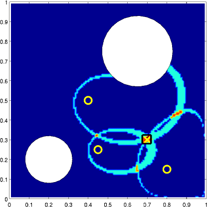
Figure 1: Sum of level set indicator functions $X(\boldsymbol{y})$ for the case of one source and three measurements. Measurement positions are yellow $\circ$, source position is yellow $\times$, source estimate $\boldsymbol{y}^{\star}$ is black $\square$.

To formulate a strategy of adaptive measurement placement we study how measurement positions affect the estimates of source location in the case of a single source. Such strategy may not be optimal, because it does not take into account the interactions between multiple sources, but it allows us to come up with a simple set of rules that can be applied if adding new measurements is relatively inexpensive. As we see in the numerical experiments in Section 4.3 such a strategy indeed proves itself useful in the case of multiple sources.

We first consider the simplest case of identifying a single source with a known intensity. Equations (2.23) then become $\boldsymbol{V}(\boldsymbol{y})=\boldsymbol{d}/\boldsymbol{a}$, with both $\boldsymbol{d}$ and $\boldsymbol{a}$ scalars. Thus, the source is located at the intersection of level sets of the components of $\boldsymbol{V}(\boldsymbol{y})$ corresponding to the value $\boldsymbol{d}/\boldsymbol{a}$. The level sets are closed curves relative to the domain $\Omega$, which is a consequence of comparison results for parabolic equations. There exists an analogy to the process of triangulation in radar detection, where the corresponding curves are circles. The analogy is exact for a linear diffusion equation in $\mathbb{R}^{2}$, for which the level set curves are circles too. To illustrate this analogy numerically we consider a problem with one source and three measurements in two dimensions (the detailed description of the system is given in Section 3). Let us introduce the indicator functions of $C$-neighborhoods of $\boldsymbol{d}/\boldsymbol{a}$ level sets

$$\chi_{k}(\boldsymbol{y})=\left\{\begin{tabular}[]{ll}1,&if $|V_{k}(\boldsymbol{y})-\boldsymbol{d}/\boldsymbol{a}|\leq C$\\ 0,&if $|V_{k}(\boldsymbol{y})-\boldsymbol{d}/\boldsymbol{a}|>C$\end{tabular}\right.,\quad k=1,\ldots,3,$$ (2.33)

for some $C>0$. Given the sum $X(\boldsymbol{y})=\sum\limits_{k=1}^{3}\chi_{k}(\boldsymbol{y})$ we can define the set $S_{3}=\left\{\boldsymbol{y}\;|\;X(\boldsymbol{y})=3\right\}$, then the position of the source can be estimated as

$$\boldsymbol{y}^{\star}=\frac{\int\limits_{S_{3}}\boldsymbol{y}\;d\boldsymbol{y}}{\int\limits_{S_{3}}d\boldsymbol{y}}.$$ (2.34)

This is shown in Figure 1 with $C=0.125$.

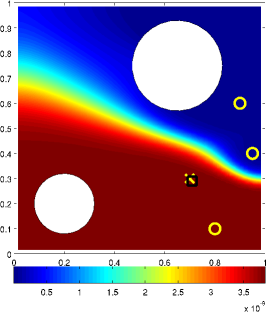
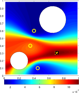
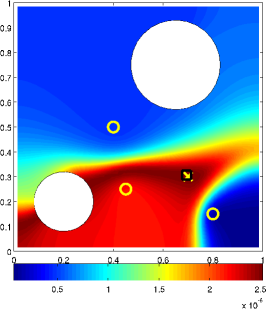
Figure 2: Imaging functional $J(\boldsymbol{r})$ from (2.31) for different measurement positions. Left: all measurements upwind. Middle: all measurements downwind. Right: mixed measurements (2 downwind and 1 upwind). Measurement positions are yellow $\circ$, source position is yellow $\times$, estimated source location (maximum of $J(\boldsymbol{r})$) is black $\square$.

For the case of exact data we can place the measurements anywhere in the domain and still be able to recover the location of the source. However, the presence of noise effectively limits the distance from the measurement to the source that allows a stable source identification. This is due to the fact that the magnitude of the measured solution $\boldsymbol{u}$ decays quickly away from the source, and measuring weak signals is more prone to errors than measuring strong signals. Thus, if a priori information about the source locations is not available, a reasonable strategy is to distribute the measurements more or less uniformly around the domain $\Omega$.

The situation is different when some prior knowledge about source locations is a available. One example is when we would like to add new measurements adaptively based on the results of source identification with a previously chosen smaller number of measurements. Here we assume that we can add new measurements anywhere in the domain and that it is relatively inexpensive to do so. This leads us to a strategy of adding a few new measurements for each previously identified source. We also assume that the sources and measurements are active for all times $t\in[0,T]$, so only the spatial placement of the measurements is considered. For a source with unknown intensity we add $d+1$ measurements, where we use $d=2$ dimensions for the convenience of visualization.

In order to distribute the newly added measurements around the previously estimated source locations we study how the distribution of measurements affects the source identification in the presence of advection in the case of a single source. In Figure 2 we plot the imaging functional for the three different measurement distribution (the details of the numerical setup are given in sections 3 and 4). The preferred advection direction in Figure 2 is from right to left, so we refer to the measurements to the right of the source as upwind and to the left of the source as downwind (see section 3.2 for a definition of a preferred advection direction). The three possible distributions given are for all three measurements upwind, all three measurements downwind and a mixed distribution of one measurement upwind and 2 downwind.

The plots in Figure 2 are for the noiseless data, so the source position is recovered exactly (up to the nearest computational grid point). However, there is a drastic difference in the behavior of the imaging functional, which allows us to identify an optimal placement of measurements. Obviously, having all measurements upwind is the worst scenario. Advection propagates the plume away from the measurements and makes source identification difficult. This is reflected in the imaging functional having a vast plateau which implies the lack of discriminatory power of such functional. Ideally an imaging functional should have a single concentrated peak at the source location. By placing all three measurements downwind the behavior of the imaging functional is much improved. The peak is now located on a narrow ridge, thus the solution is expected to be less susceptible to noise. Finally, we observe that having one measurement upwind can further improve the imaging functional since it allows for exclusion of a portion of the domain from possible source locations (the imaging functional is small around the upwind source).

Considering the above observations we propose the following procedure for adaptive measurement placement.

Algorithm 4 (Geometric adaptive measurements placement).

1. Obtain an estimate of source locations $\boldsymbol{y}$.

2. Choose a trust radius $\rho_{T}$ and a reference simplex $\boldsymbol{T}$ with vertices $\boldsymbol{T}^{k}$, $k=1,\ldots,d+1$. The orientation of the reference simplex is such that one vertex lies upwind and $d$ vertices lie downwind from its center (the center of circumscribed sphere).

3. For $j=1,\ldots,N_{s}$ do

4. Place the center of the reference simplex at $\boldsymbol{y}^{j}$.

5. For $k=1,\ldots,d+1$ do

   1. Place a new measurement in the direction of the vertex $\boldsymbol{T}^{k}$ at a distance

      $$\rho=\min\left(\rho_{T},\kappa_{\Omega}\;\mbox{dist}\left(\boldsymbol{y}^{j},\partial\Omega\right),\kappa_{\boldsymbol{y}}\;\mbox{dist}\left(\boldsymbol{y}^{j},\left\{\boldsymbol{y}^{i}\;|\;i\neq j\right\}\right)\right)$$ (2.35)

      away from $\boldsymbol{y}^{j}$, where the constants $\kappa_{\Omega},\kappa_{\boldsymbol{y}}\in(0,1)$ determine how close the new measurements can be placed to the boundary and the rest of the sources respectively.

6. For $i=1,\ldots,j-1$ do

   1. Place a new measurement on a line connecting $\boldsymbol{y}^{j}$ and $\boldsymbol{y}^{i}$.

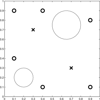
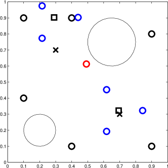
Figure 3: Numerical example of performance of Algorithm 4. Problem with $N_{s}=2$ sources (black $\times$) and $N_{m}=6$ initial measurements (black $\circ$). Left: initial measurement distribution. Right: source location estimates (black $\square$) with noisy data ($5\%$ noise) and measurement locations added adaptively by Algorithm 4 (blue and red $\circ$). Measurement locations added for better refinement in step (iv) are in blue, and that added in step (v) for improved separation is in red.

The choice of a trust radius $\rho_{T}$ in step (ii) should be determined by the noise level, i.e. the distance from the source to the measurements for which the source can be identified in a stable manner. In two dimensions the algorithm places three new measurements per identified source in a triangular pattern around each source so that one measurement is placed upwind and two downwind. Relation (2.35) ensures that the new measurements are not placed too close to the boundary or to other sources. This helps to separate the sources in case they are clustered together. Adding measurements in step (v) also helps separating clustered sources. It is possible to adjust the shape of the reference simplex $\boldsymbol{T}$ in step (v) and the positioning of the measurements in step (v) to take into account the knowledge of the advection field. However, for simplicity in the numerical examples in Section 4 we use an equilateral triangle $\boldsymbol{T}$ in step (ii) and $\boldsymbol{z}=(\boldsymbol{y}^{j}+\boldsymbol{y}^{i})/2$ in step (v).

We illustrate the behavior of Algorithm 4 numerically in Figure 3. We first obtain the estimates of the locations of two time-independent sources based on a minimal number of measurements (six) using Algorithm 1. Algorithm 4 then adds seven more measurements (six in step (iv) and one in step (v)). Note that source identification is performed with noisy data, so the initial estimate for the top left source is off the true location. However, after more measurements are added adaptively, both sources may be recovered correctly. This is shown in the numerical experiments in section 4.3 (see Figure 6).

Note that Algorithm 4 is based on the idea of local refinement, i.e. the new measurements are placed near the estimated source positions. Such approach is in agreement with the successive sampling strategy developed in [17], which gives good results for source identification in $L_{1}$ setting. For each discovered source Algorithm 4 adds new measurements redundantly, which may not be the most efficient way if each new measurement is expensive in some sense (expensive sensors, placement in remote locations, etc). As an alternative we propose an algorithm that is based on using the level sets of adjoint solutions. Below is a simple version of the algorithm that adds one new measurement at a time.

Algorithm 5 (Level set adaptive measurements placement).

1. For every possible measurement location $\boldsymbol{z}\in\Omega$ form a corresponding term $\boldsymbol{g}^{\boldsymbol{z}}$ and solve the adjoint system

   $$-\boldsymbol{v}^{\boldsymbol{z}}_{t}=(\boldsymbol{D}\boldsymbol{\Delta}+\boldsymbol{w}\cdot\boldsymbol{\nabla}+\boldsymbol{L}^{T}+\boldsymbol{Q}^{T}(\boldsymbol{u}^{q}))\boldsymbol{v}^{\boldsymbol{z}}+\boldsymbol{g}^{\boldsymbol{z}},$$

   with the reaction term fixed around the last estimate $\boldsymbol{u}^{q}$ of the forward-adjoint iteration.

2. Select the signal level $\epsilon$ that can be measured stably.

3. Define the indicator functions of $\epsilon$-level sets

   $$\chi_{\boldsymbol{z}}^{\epsilon}(\boldsymbol{x})=\left\{\begin{tabular}[]{ll}$1$,&$v_{k}^{\boldsymbol{z}}(\boldsymbol{x})\geq\epsilon$\\ $0$,&$v_{k}^{\boldsymbol{z}}(\boldsymbol{x})<\epsilon$\end{tabular}\right.,\quad\boldsymbol{x}\in\Omega,$$ (2.36)

   where $k$ is the index of the component of $\boldsymbol{f}$ that contains the (single) source.

4. Define the set

   $$S_{\boldsymbol{z}}^{\epsilon}=\{\boldsymbol{x}\in\Omega\;|\;\sum_{i=1}^{N_{m}}\chi_{\boldsymbol{z}_{i}}^{\epsilon}(\boldsymbol{x})+\chi_{\boldsymbol{z}}^{\epsilon}(\boldsymbol{x})\geq 2\}$$ (2.37)

   for every $\boldsymbol{z}\in\Omega$.

5. The new measurement $\boldsymbol{z}^{\star}$ is a solution of a constrained optimization problem

   $$\boldsymbol{z}^{\star}=\mathop{\mbox{argmax}}\limits_{\mbox{s.t. }\chi_{\boldsymbol{z}}^{\epsilon}(\boldsymbol{y}^{q})=1}\int_{S_{\boldsymbol{z}}^{\epsilon}}d\boldsymbol{x}$$ (2.38)

Algorithm 5 is based around the idea of a region of stable identification. In the presence of noise in the measured data we define in step (ii) of the algorithm the signal level $\epsilon$ that can be measured stably. Thus, at each measurement location $\boldsymbol{z}\in\Omega$ a signal from a source located in the level set $\{\boldsymbol{x}\in\Omega\;|\;\chi_{\boldsymbol{z}}^{\epsilon}(\boldsymbol{x})=1\}$ can be stably measured. Since a source can only be identified with multiple measurements, in the construction of $S_{\boldsymbol{z}}^{\epsilon}$ in step (iv) of the algorithm we require that two or more level sets from the measurements at existing ($\boldsymbol{z}_{i}$) and trial ($\boldsymbol{z}$) locations intersect. Then, the best location for a newly added measurement $\boldsymbol{z}^{\star}$ is the one that maximizes the coverage of $\Omega$ by such intersecting level sets, i.e. maximizes the area of $S_{\boldsymbol{z}}^{\epsilon}$, which is the objective of (2.38). A reasonable constraint to have in the optimization problem (2.38) is that the estimate $\boldsymbol{y}^{q}$ from the forward-adjoint iteration with $N_{m}$ previously made measurements belongs to the level set of a newly added measurement.

We present a numerical example of performance of Algorithm 5 in Figure 4. In this example we consider the case of three upwind measurements shown in the leftmost plot in Figure 2. The method performs as expected, i.e. it places the newly added measurement $\boldsymbol{z}^{\star}$ downwind from the source location $\boldsymbol{y}^{q}$ estimated by Algorithm 1 using three previously made measurements. To find the solution of the optimization problem (2.38) we use a direct search over a number of trial measurement locations. The values of the objective of (2.38) at those locations are shown on the right in Figure 4. Although the objective is not convex, its behavior is quite regular, so other optimization techniques can be employed. Note that the evaluation of the objective of (2.38) requires the computation of $\boldsymbol{v}^{\boldsymbol{z}}$ and thus the optimization problem can become quite expensive to solve if multiple evaluations of the objective are required. This is in contrast with the geometric approach of Algorithm 4 that does not require any adjoint or forward solves. Algorithm 4 is also easier to use in case when the addition of several new measurements at the same time is needed. These differences determine the settings in which the use of either algorithm is more beneficial. Algorithm 4 is advantageous when multiple measurements need to be placed and the price associated with deploying them is low, so some degree of redundancy can be tolerated. When placing a new measurement is expensive it is beneficial to use Algorithm 5 for carefully choosing an optimal location.

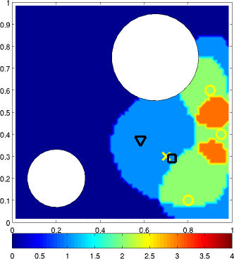
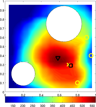
Figure 4: Numerical example of performance of Algorithm 5. Problem with a single source (yellow $\times$) and three measurements upwind (yellow $\circ$, same as the leftmost example in Figure 2). Left: $\sum_{i=1}^{N_{m}}\chi_{\boldsymbol{z}_{i}}^{\epsilon}(\boldsymbol{x})+\chi_{\boldsymbol{z}}^{\epsilon}(\boldsymbol{x})$ from (2.37). Right: objective $\int_{S_{\boldsymbol{z}}^{\epsilon}}d\boldsymbol{x}$ of (2.38). Source estimate $\boldsymbol{y}^{q}$ from Algoritm 1 is black $\square$. Newly added measurement location $\boldsymbol{z}^{\star}$ is black $\bigtriangledown$.

We conclude this section by considering the problem of determining an unknown number of sources, the case when $N_{s}$ is not known a priori. A procedure that appears to be both simple and reliable if to start with and estimated number of sources $N_{s}^{*}=1$ and run Algorithm 1 repeatedly for increasing numbers $N_{s}^{*}=2,3,\ldots$. Note that the optimization problem (2.28) does not impose any constraints on the signs of components of $\boldsymbol{a}$. Thus, for some value of $N_{s}^{*}$ Algorithm 1 will compute a solution with $a_{j}=0$ for some $j$ in the noiseless case, or in the presence of noise $a_{j}\leq\epsilon$ (this includes negative $a_{j}$) for some small $\epsilon$, which should be chosen based on noise level. Once this happens we determine the true number of sources as $N_{s}=N_{s}^{*}-1$. The choice of the number of measurements in the case of unknown $N_{s}$ can be done in two ways. If an upper bound $N_{s}<N_{s}^{\mbox{max}}$ is available one may set $N_{m}$ to the number of measurements needed to identify $N_{s}^{\mbox{max}}$ sources stably. Alternatively, one may add the measurements adaptively using Algorithms 4 or 5 for each value of $N_{s}^{*}$. In the numerical experiments in Section 4.4 we use the former approach.

3 Three component chemical system

In this section we consider a system that we use in the numerical experiments in Section 4. We use a simplified, but somewhat realistic three component $n=3$ chemical system that models the chemical processes occurring in the atmosphere based on Chapman’s cycle [20, 16]. While a realistic atmospheric model may contain dozens of reacting species [12], our simple model still captures some of the basic features of atmospheric models like polynomial non-linearity and stiffness.

3.1 Forward problem

The components of the system are the nitric oxide ($NO$), nitrogen dioxide ($NO_{2}$) and ozone ($O_{3}$) denoted by $u_{1}$, $u_{2}$ and $u_{3}$ respectively. We assume that nitrogen dioxide is released at source locations and the concentrations of nitric oxide are measured. A simplified model of chemical reactions in the system is

$$NO+O_{3} \mathrel{\mathop{\hbox to18.8888pt{\hbox{$\displaystyle\relbar\mkern-7.0mu\cleaders\hbox{$\displaystyle\mkern-2.0mu\relbar\mkern-2.0mu$}\hfill\mkern-7.0mu\rightarrow$}}}\limits^{k_{1}\mkern 3.0mu}} NO_{2},$$ (3.39)

$$NO_{2} \mathrel{\mathop{\hbox to18.8888pt{\hbox{$\displaystyle\relbar\mkern-7.0mu\cleaders\hbox{$\displaystyle\mkern-2.0mu\relbar\mkern-2.0mu$}\hfill\mkern-7.0mu\rightarrow$}}}\limits^{k_{2}\mkern 3.0mu}} NO+O_{3},$$ (3.40)

with rates $k_{1}=1000$, $k_{2}=2000$. Let us introduce a scalar reaction term

$$r(\boldsymbol{u})=k_{1}u_{1}u_{3}-k_{2}u_{2},$$ (3.41)

then the vector reaction term is given by

$$\boldsymbol{R}(\boldsymbol{u})=\left[\hskip-5.0pt\begin{array}[]{*\c@MaxMatrixCols c}-r(\boldsymbol{u})\\ \>\>\>r(\boldsymbol{u})\\ -r(\boldsymbol{u})\end{array}\hskip-5.0pt\right]=\boldsymbol{L}\boldsymbol{u}+\boldsymbol{Q}(\boldsymbol{u})\boldsymbol{u},$$ (3.42)

where we take

$$\boldsymbol{L}=\left[\hskip-5.0pt\begin{array}[]{*\c@MaxMatrixCols c}0&\>\>\>k_{2}&0\\ 0&-k_{2}&0\\ 0&\>\>\>k_{2}&0\end{array}\hskip-5.0pt\right],\quad\boldsymbol{Q}(\boldsymbol{u})=\left[\hskip-5.0pt\begin{array}[]{*\c@MaxMatrixCols c}-k_{1}u_{3}&0&0\\ \>\>\>k_{1}u_{3}&0&0\\ 0&0&-k_{1}u_{1}\end{array}\hskip-5.0pt\right].$$ (3.43)

Note that while the linear part $\boldsymbol{L}$ is defined uniquely, different definitions of the quadratic part $\boldsymbol{Q}$ are possible that lead to the same value of the matrix-vector product $\boldsymbol{Q}(\boldsymbol{u})\boldsymbol{u}$ and thus the same reaction term.

The realistic values of the diffusion constants are $\epsilon_{1}=1$, $\epsilon_{2}=\epsilon_{3}=5$, which lead to a rather stiff system of equations due to large contrast between the diffusion constants and the reaction rates $k_{1}$, $k_{2}$.

While our method works in any number of spatial dimensions, in this numerical example we use $d=2$ dimensions for the simplicity of visualization. The system is solved in the unit square with circular obstacles

$$\Omega=[0,1]^{2}\setminus\left(\bigcup_{j=1}^{N_{o}}B_{r_{j}}(\boldsymbol{c}_{j})\right),$$ (3.44)

where $N_{o}$ is a number of obstacles. In the example below we take $N_{o}=2$. Dirichlet conditions are enforced on the outer boundary

$$\left.u_{1}\right|_{\partial[0,1]^{2}}=\left.u_{2}\right|_{\partial[0,1]^{2}}=0,\quad\left.u_{3}\right|_{\partial[0,1]^{2}}=1,$$ (3.45)

and zero Neumann conditions are enforced on the obstacle boundaries

$$\left.\frac{\partial u_{j}}{\partial\nu}\right|_{\partial B_{r_{k}}(\boldsymbol{c}_{k})}=0,\quad j=1,\ldots,n,\quad k=1,\ldots,N_{o}.$$ (3.46)

Constant initial conditions are used

$$\left.u_{1}\right|_{t=0}=\left.u_{2}\right|_{t=0}=0,\quad\left.u_{3}\right|_{t=0}=1.$$ (3.47)

We assume that at $t=0$ all sources go off and remain active for the period of time $[0,T]$. The source term has the form

$$\boldsymbol{f}(\boldsymbol{x})=\left[\hskip-5.0pt\begin{array}[]{*\c@MaxMatrixCols c}0\\ \sum\limits_{j=1}^{N_{s}}a_{j}\delta(\boldsymbol{x}-\boldsymbol{y}^{j})\\ 0\end{array}\hskip-5.0pt\right],$$ (3.48)

so only the source locations $\boldsymbol{y}^{j}\in\Omega$ and the constant source intensities $a_{j}>0$ are to be determined.

3.2 Advection field

A realistic assumption on the advection term is that there exists a preferred advection direction $\boldsymbol{w}_{0}$ that does not depend on time. It is also reasonable to assume that the advection vector field satisfies non-penetrating boundary conditions on the boundaries of the obstacles

$$\left.(\boldsymbol{w}\cdot\nu)\right|_{\partial B_{r_{j}}(\boldsymbol{c}_{j})}=0,\quad j=1,\ldots,N_{o}.$$ (3.49)

Let us introduce the advection potential $\phi$ such that

$$\boldsymbol{w}=\nabla\phi.$$ (3.50)

Then the condition that the advection vector field is divergence free implies that $\phi$ must be harmonic

$$\Delta\phi=0\quad\mbox{in }\Omega,$$ (3.51)

with zero Neumann boundary conditions on the obstacle boundaries

$$\left.\frac{\partial\phi}{\partial\nu}\right|_{\partial B_{r_{j}}(\boldsymbol{c}_{j})}=0,\quad j=1,\ldots,N_{o},$$ (3.52)

and Neumann conditions enforcing the preferred direction on the outer boundaries

$$\left.\frac{\partial\phi}{\partial\nu}\right|_{\partial[0,1]^{2}}=\left.(\boldsymbol{w}_{0}\cdot\nu)\right|_{\partial[0,1]^{2}}.$$ (3.53)

Advection field used in the numerical examples below corresponds to a preferred advection direction $\boldsymbol{w}_{0}=(-50,0)$, i.e. the “wind” blows from right to left.

3.3 Measurements and the adjoint system

For the three component chemical system we measure the component $u_{1}$. In the numerical results below we consider the cases of measurements integrated in time (sections 4.3 and 4.4) and of instantaneous measurements (Section 4.5). The term $\boldsymbol{g}$ in the adjoint system (2.16) for the $i^{th}$ measurement takes the form

$$\boldsymbol{g}^{(i)}(\boldsymbol{x})=\left[\hskip-5.0pt\begin{array}[]{*\c@MaxMatrixCols c}\delta(\boldsymbol{x}-\boldsymbol{z}^{i})\\ 0\\ 0\end{array}\hskip-5.0pt\right],\mbox{ or}\quad\boldsymbol{g}^{(i)}(\boldsymbol{x})=\left[\hskip-5.0pt\begin{array}[]{*\c@MaxMatrixCols c}\delta(t-\theta_{i})\delta(\boldsymbol{x}-\boldsymbol{z}^{i})\\ 0\\ 0\end{array}\hskip-5.0pt\right],\quad i=1,\ldots,N_{m}.$$ (3.54)

for integrated or instantaneous measurements respectively.

While the initial and boundary conditions for the forward system typically come from the physical problem, we have a freedom of choosing the terminal and boundary conditions for the adjoint system, so that the adjoint relation (2.20) is as simple as possible. In particular, we would like the correction term (2.1) to be zero. We enforce zero Dirichlet conditions on the outer boundary and zero Neumann conditions on the obstacle’s boundaries for all three components of the adjoint solution $\boldsymbol{v}$. We also use zero terminal condition $\boldsymbol{v}(\boldsymbol{x},T)=0$, $\boldsymbol{x}\in\Omega$.

From the expression (3.43) for $\boldsymbol{L}$ and $\boldsymbol{Q}(\boldsymbol{u})$ we obtain the equation for the third component of the adjoint solution

$$-v_{3,t}=\left(\epsilon_{3}\Delta-\boldsymbol{w}\cdot\nabla-k_{1}u_{1}\right)v_{3}.$$ (3.55)

Combined with the terminal and boundary conditions we immediately see that

$$v_{3}(\boldsymbol{x},t)\equiv 0,\quad\boldsymbol{x}\in\Omega,\quad t\in[0,T].$$ (3.56)

This is enough to make the correction term (2.1) zero. Indeed, the only component of $\boldsymbol{u}$ and $\boldsymbol{v}$ that has non-zero initial (terminal) or boundary conditions is $u_{3}$. Since $v_{3}$ is identically zero it neutralizes non-zero initial and boundary conditions for $u_{3}$ in the first three terms of the $c(\boldsymbol{u},\boldsymbol{v})$. There is no contribution from the other components of $\boldsymbol{u}$, and $\boldsymbol{v}$ to the first three terms, so they are identically zero. The fourth term is zero since we use a divergence free advection field $\boldsymbol{w}$. Finally, the fifth term on the outer boundary is taken care of because $\left.\boldsymbol{v}\right|_{\partial[0,1]^{2}}=0$. On the boundaries of the obstacles it is zero since $\boldsymbol{w}$ satisfies the non-penetrating conditions (3.49) there.

Once we establish that $c(\boldsymbol{u},\boldsymbol{v})$ is zero we can write the components of the system of equations (2.23) arising from the adjoint relation

$$V_{ik}=\int_{0}^{T}v_{2}^{(i)}(\boldsymbol{y}^{k},t)dt, V_{ik}=v_{2}^{(i)}(\boldsymbol{y}^{k},\tau_{k}),$$ or (3.57)

$$d_{i}=\int_{0}^{T}u_{1}(\boldsymbol{z}^{i},t)dt, d_{i}=u_{1}(\boldsymbol{z}^{i},\theta_{i}),$$ or (3.58)

for integrated or instantaneous measurements respectively, where $i=1,\ldots,N_{m}$, $k=1,\ldots,N_{s}$ and

$$\boldsymbol{a}=\left(a_{1},\ldots a_{N_{s}}\right)^{T},$$ (3.59)

is the same for both cases.

4 Numerical results

We implement our method of source identification and provide the results of the numerical experiments below. The first two sets of experiments use time integrated measurements as described in Section 3.3. In these experiments we identify time-independent sources in the cases where the number of sources itself is known (Section 4.3) or unknown (Section 4.4). In Section 4.3 we also study adaptive positioning of measurements and its influence on source identification. Finally, in Section 4.5 we provide the numerical results for identification of a time dependent source from instantaneous measurements. Results from both one and two dimensional settings are presented.

4.1 Linear parabolic solver

We solve the linear parabolic systems for the forward and adjoint iterations using the following numerical schemes. The spatial part is discretized with finite differences on a uniform Cartesian grid. The two-dimensional Laplace operator in the diffusion term is discretized using the standard five-point stencil. The advection term is discretized using a central difference scheme. The reason for using the central difference scheme for the advection term is that we can use the same discretization for the forward and adjoint problem, for which the direction of advection is reversed. Note that such discretization may become inaccurate if the advection dominates other terms. While there exist more sophisticated and accurate numerical schemes for the solution of advection-diffusion equations, the focus of this work is not the numerical solution of the forward problem. The numerical scheme described in this section appears to be sufficiently accurate for source identification in a three component system described in Section 3.

To obtain the solution in time we use an exponential integrator. After discretizing in space we need to solve the system of ODEs for the forward and adjoint problems of the following form

$$\boldsymbol{\xi}_{t}=\boldsymbol{E}(t)\boldsymbol{\xi}+\boldsymbol{\zeta}(t).$$ (4.60)

The dependency of the matrix $\boldsymbol{E}$ on time is due to the fact that the reaction term $\boldsymbol{Q}$ depends on the forward solution that is a function of time. If we denote the $k^{th}$ time step by $t_{k}$ and the size of the step is $h_{k}=t_{k+1}-t_{k}$, then the approximate solution at time step $k+1$ is given by

$$\boldsymbol{\xi}^{(k+1)}=\mbox{exp}\left(\boldsymbol{E}^{(k)}h_{k}\right)\left(\left(\boldsymbol{E}^{(k)}\right)^{-1}\boldsymbol{\zeta}^{(k)}+\boldsymbol{\xi}^{(k)}\right)-\left(\boldsymbol{E}^{(k)}\right)^{-1}\boldsymbol{\zeta}^{(k)},$$ (4.61)

where $\boldsymbol{\xi}^{(k)}\approx\boldsymbol{\xi}(t_{k})$, $\boldsymbol{E}^{(k)}=\boldsymbol{E}(t_{k})$ and $\boldsymbol{\zeta}^{(k)}=\boldsymbol{\zeta}(t_{k})$. While each step of this method is more computationally expensive than that of traditional time stepping methods, it is more accurate allowing us to use a small number of time steps. Note that (4.61) requires evaluation of matrix-vector products with matrix exponentials. We evaluate these products using an efficient algorithm [2].

In order to avoid committing an inverse crime [7] we use different grid and time steps for the forward problem data simulation and for the solution of the source identification problem with Algorithm 1. We simulate the data on a finer grid with $80$ grid nodes in both $x$ and $y$ directions and $30$ time steps. In the case of time independent source and integrated measurements we perform source identification on a grid with $63$ grid nodes in both $x$ and $y$ directions and $19$ time steps.

Note that even without adding artificially generated noise to the data, using different (and relatively coarse) grids for the data simulation and source identification is equivalent to having some systematic error in the measurements. This poses an issue in the case of time dependent source and instantaneous measurements, since this case is more sensitive to the noise level in the data. In this case we use a finer grid for source identification, namely with $73$ nodes in both directions. Another modification to the solver required in this case is the use of non-uniform time stepping. In order to properly resolve the singularity of the sources around times $\tau_{k}$, $k=1,\ldots,N_{s}$ in the forward problem and around $\theta_{j}$, $j=1,\ldots,N_{m}$ in the adjoint problems, we refine the time stepping locally.

4.2 Noise model

We provide below the results of the numerical experiments for identifying sources from noisy measurements. Single source identification with noiseless measurements can be found in Figure 2. In this section we use a simple noise model with multiplicative normally distributed noise. Such model while being easy to implement captures a realistic assumption that the noise level can be viewed as constant relative to the strength of the signal.

If we denote the simulated data vector by $\boldsymbol{d}$, then the noisy data $\boldsymbol{d}^{*}$ is given by

$$\boldsymbol{d}^{*}=(\boldsymbol{I}+\sigma\boldsymbol{N})\boldsymbol{d},\quad\boldsymbol{N}=\mbox{diag}\left(X_{1},\ldots,X_{N_{m}}\right),$$ (4.62)

where $\sigma$ is a scaling term and $X_{j}$, $j=1,\ldots,N_{m}$ are independent normally distributed random variables with zero mean and unit standard deviation. All results are presented for one particular realization of noise, although for different realizations the results remain similar, which indicates that the source identification Algorithm 1 is relatively stable.

In the case of time-independent sources and integrated measurements we take the scaling factor $\sigma=0.05$ corresponding to $5\%$ relative noise level. Note that according to (4.62) the noise is added to the data after the integration in (3.58). Adding the noise to $u_{1}$ before the integration in (3.58) would make it easier for Algorithm 1 to determine the source, since integration in (3.58) would act as a noise canceling filter. In order to stress test our method we add the noise after the integration instead. As a measure of error in the solution we use a relative location error given by

$$E=\frac{1}{lN_{s}}\sum_{j=1}^{N_{s}}\|\boldsymbol{y}^{j}-\widehat{\boldsymbol{y}}^{j}\|,$$ (4.63)

where $\boldsymbol{y}^{j}$ are the estimates and $\widehat{\boldsymbol{y}}^{j}$ are the true source locations. The characteristic length $l$ is set here to $l=1$ since our domain is the unit square with obstacles.

The case of time dependent source and instantaneous measurements is more difficult. Accordingly, we reduce the noise level to $\sigma=0.01$ for the numerical experiments in Section 4.5.

4.3 Identifying multiple sources with adaptive measurement placement

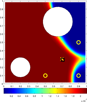
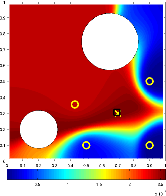
Figure 5: Imaging functional $J(\boldsymbol{r})$ for all $\boldsymbol{r}\in\Omega$ given by the final iteration of Algorithm 1. Right: initial run with $N_{m}=3$ measurements. Left: subsequent run with an extra measurement added adaptively by Algorithm 5. True source location is yellow $\times$, measurement locations are yellow $\circ$, estimated source position $\boldsymbol{y}$ - maximum of the imaging functional is black $\square$.

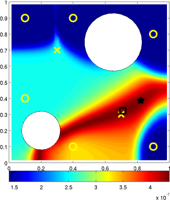
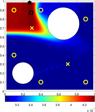
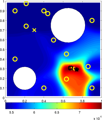
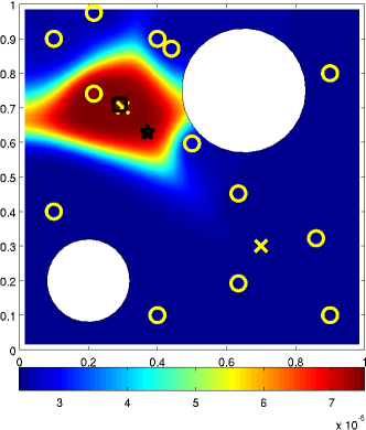
Figure 6: Imaging functionals $J(\boldsymbol{r},\boldsymbol{y}^{2})$ (left column) and $J(\boldsymbol{y}^{1},\boldsymbol{r})$ (right column) from (2.30) for all $\boldsymbol{r}\in\Omega$ evaluated at the final value of $(\boldsymbol{y}^{1},\boldsymbol{y}^{2})$ given by Algorithm 1. Top row: initial run with $N_{m}=6$ measurements. Bottom row: subsequent run with measurements added adaptively by Algorithm 4 ($N_{m}=13$). True source locations are yellow $\times$, measurement locations are yellow $\circ$, estimated source position $(\boldsymbol{y}^{1},\boldsymbol{y}^{2})$ - maximum of the imaging functional is black $\square$, initial guess from Algorithm 3 is black $\star$.

Table 1: True and reconstructed source intensities $a_{j}$ and locations $\boldsymbol{y}^{j}$, and relative location errors $E$ for the case of two sources ($5\%$ noise in the data).

• Case	$a_{1}$	$a_{2}$	$\boldsymbol{y}^{1}$	$\boldsymbol{y}^{2}$	$E$
  True	10.00	7.00	(0.70, 0.30)	(0.30, 0.70)	–
  $N_{m}=6$	13.37	2.27	(0.70, 0.32)	(0.29, 0.87)	0.09
  $N_{m}=13$	9.62	6.44	(0.67, 0.30)	(0.29, 0.70)	0.02

In this section we study the identification of a known number of time independent sources from integrated measurements in a three component system from Section 3. We consider three cases $N_{s}=1,2,3$ in Figures 5, 6 and 7 respectively. To demonstrate the adaptive measurement placement we begin by choosing the smallest number of measurements $N_{m}=3N_{s}$ that yields a formally determined system (2.23). Then we add more measurements using Algorithm 5 in the case $N_{s}=1$ and Algorithm 4 for $N_{s}=2,3$. Then we run Algorithm 1 again with the adaptively added measurements. For the purposes of visualization for the $j^{th}$ source we fix $k^{th}$ source locations given by Algorithm 1 for all $k\neq j$ and evaluate the functional (2.30) for all possible locations of the $j^{th}$ source in $\Omega$. This is similar to step (ii) of Algorithm 2. Obviously, the maximum of the functional corresponds to the source location estimated by Algorithm 1. Doing so allows us to visualize the sensitivity of the objective of (2.25) with respect to the location of the $j^{th}$ source and also how it changes when more measurements are added adaptively.

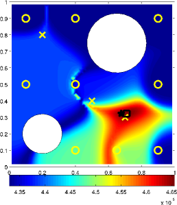
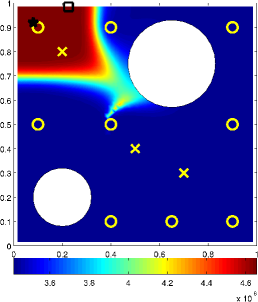
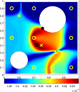
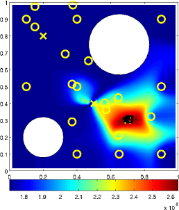
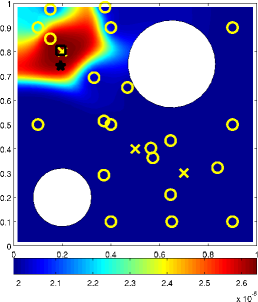
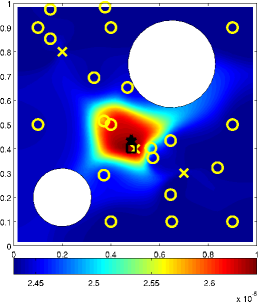
Figure 7: Imaging functionals $J(\boldsymbol{r},\boldsymbol{y}^{2},\boldsymbol{y}^{3})$ (left column), $J(\boldsymbol{y}^{1},\boldsymbol{r},\boldsymbol{y}^{3})$ (middle column) and $J(\boldsymbol{y}^{1},\boldsymbol{y}^{2},\boldsymbol{r})$ (right column) from (2.30) for all $\boldsymbol{r}\in\Omega$ evaluated at the final value of $(\boldsymbol{y}^{1},\boldsymbol{y}^{2},\boldsymbol{y}^{3})$ given by Algorithm 1. Top row: initial run with $N_{m}=9$ measurements. Bottom row: subsequent run with measurements added adaptively by Algorithm 4 ($N_{m}=21$). True source locations are yellow $\times$, measurement locations are yellow $\circ$, estimated source position $(\boldsymbol{y}^{1},\boldsymbol{y}^{2},\boldsymbol{y}^{3})$ - maximum of the imaging functional is black $\square$, initial guess from Algorithm 3 is black $\star$.

Table 2: True and reconstructed source intensities $a_{j}$ and locations $\boldsymbol{y}^{j}$, and relative location errors $E$ for the case of three sources ($5\%$ noise in the data).

Case	$a_{1}$	$a_{2}$	$a_{3}$	$\boldsymbol{y}^{1}$	$\boldsymbol{y}^{2}$	$\boldsymbol{y}^{3}$	$E$
True	10.00	7.00	5.00	(0.70, 0.30)	(0.20, 0.80)	(0.50, 0.40)	–
$N_{m}=9$	13.06	21.42	4.22	(0.70, 0.32)	(0.22, 0.98)	(0.43, 0.40)	0.09
$N_{m}=21$	9.35	7.26	5.31	(0.70, 0.30)	(0.19, 0.80)	(0.48, 0.40)	0.01

Detection of a single source is rather robust, so even in the presence of measurement noise the source is identified almost exactly with just three measurements, as is illustrated in the left plot in Figure 5. However, the imaging functional has a large plateau around the true source location due to lack of downwind measurements. Algorithm 5 performs as expected by adding a new measurement downwind and the imaging functional becomes much better localized as shown in the right plot in Figure 5.

In Figure 6 we observe that the objective is not convex (the functional $J$ is not concave). Also in Figure 6 for $N_{m}=9$ measurements it is clear that the objective can develop narrow valleys (ridges of $J$) and become multimodal. This makes the multiple source identification problem difficult to solve, and we observe that in the presence of noise the estimated source location may differ from the true one if too few measurements are used. In particular, we see in top rows of Figures 6 and 7 that the estimated locations are off for the sources for which the objective has a large plateau around the true location.

In Figures 6 and 7 we only show the estimated locations of the sources. The corresponding source intensities (and the numerical values for the locations) are given in Tables 1 and 2 for the cases $N_{s}=2$ and $N_{s}=3$ respectively. From the presented data we observe that the least squares estimate (2.27) of source intensities is quite sensitive to the estimate of the source locations. When few measurements are used and the estimates of the locations are not accurate enough the estimated intensities differ significantly from the true values. However, when more measurements are added adaptively, the intensity estimates improve greatly. Note that this limitation of our method comes from the fact that in (2.27) we eliminate the source intensities from the optimization variables. If we have some a priory knowledge about the intensities (i.e. the bounds) we can retain $\boldsymbol{a}$ as an optimization variable in (2.25) and enforce our a priori knowledge as a constraint. This comes at a price of enlarging the space of optimization variables, which makes the optimization problem harder to solve.

4.4 Source identification for an unknown number of sources

Let us now consider source identification in the case when a true value of $N_{s}$ is unknown. Similarly to the previous section we identify time independent sources from integrated measurements. To identify the sources and their number we use the procedure from Section 2.3. To simplify the exposition in this section we do not add the measurements adaptively. Instead we use a predetermined large number of measurements for all trial values of $N_{s}^{*}$. The measurements are distributed somewhat uniformly in $\Omega$, as shown in Figure 8.

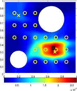
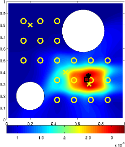
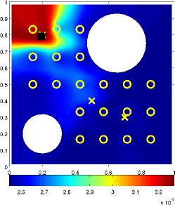
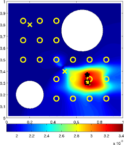
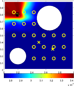
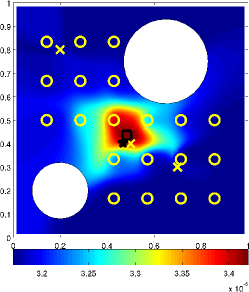
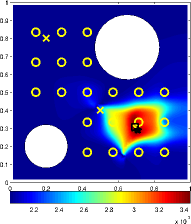
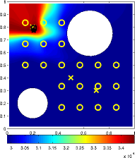
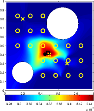
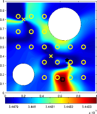
Figure 8: Unknown number of sources, the true value is $N_{s}=3$. Imaging functionals evaluated at the final value of $(\boldsymbol{y}^{1},\ldots,\boldsymbol{y}^{N_{s}^{*}})$ given by Algorithm 1. Top row: $N_{s}^{*}=1$ (leftmost) and $N_{s}^{*}=2$ (middle and right). Middle row: $N_{s}^{*}=3$. Bottom row: $N_{s}^{*}=4$. Number of measurements $N_{m}=20$ for all $N_{s}^{*}$. True source locations are yellow $\times$, measurement locations are yellow $\circ$, estimated source positions $(\boldsymbol{y}^{1},\ldots,\boldsymbol{y}^{N_{s}^{*}})$ - maxima of the corresponding imaging functional are black $\square$, initial guesses from Algorithm 3 are black $\star$.

Table 3: True and reconstructed source intensities $a_{j}$ and locations $\boldsymbol{y}^{j}$ for the case of unknown number of sources ($5\%$ noise in the data).

Case	$a_{1}$	$a_{2}$	$a_{3}$	$a_{4}$	$\boldsymbol{y}^{1}$	$\boldsymbol{y}^{2}$	$\boldsymbol{y}^{3}$	$\boldsymbol{y}^{4}$
True ($N_{s}=3$)	10.00	7.00	5.00	–	(0.70, 0.30)	(0.20, 0.80)	(0.50, 0.40)	–
$N_{s}^{*}=1$	12.29	–	–	–	(0.67, 0.35)	–	–	–
$N_{s}^{*}=2$	12.12	8.13	–	–	(0.67, 0.33)	(0.19, 0.79)	–	–
$N_{s}^{*}=3$	10.44	6.83	4.44	–	(0.69, 0.30)	(0.19, 0.80)	(0.48, 0.43)	–
$N_{s}^{*}=4$	11.30	6.42	4.12	-0.17	(0.69, 0.30)	(0.20, 0.79)	(0.48, 0.41)	(0.62, 0.14)

We set $N_{s}=3$ and we perform four trials $N_{s}^{*}=1,2,3,4$. The results of these trials along with the true source parameters are given in Table 3 and are visualized in Figure 8. We observe that as we increase the the trial number $N_{s}^{*}$ Algorithm 1 starts to “notice” the sources with smaller intensity. At the first step $N_{s}^{*}=1$ it picks the dominant source with $a_{1}=10$. At the second step it notices the presence of the source with $a_{2}=7$. Note that the locations and intensities of the first two sources are not determined exactly, because the objective of (2.28) is different from the true one unless $N_{s}^{*}=N_{s}$. However, the estimates of the locations and intensities of the first two sources while not exact are quite accurate, as can be observed in the first row of Figure 8 and also in Table 3.

Finally, when we reach $N_{s}^{*}=N_{s}=3$ the method identifies all three sources quite reliably given the level of noise present. As we go one step further $N_{s}^{*}=4$ Algorithm 1 recovers a spurious source with a negative intensity, which we use as a stopping criterion. We conclude that the true sources were recovered in the previous step and the true number of sources is $N_{s}=3$. Note that while a spurious source appears in the case $N_{s}^{*}=4$, the method gives a good estimate of the locations and intensities of the three sources. We observed such behavior for many realizations of the noise, so the results presented in Figure 8 and Table 3 are representative of the general performance of the method.

4.5 Time dependent source identification

In the numerical examples considered above we used time independent sources that are active for all $t$ in $[0,T]$. In this section we apply Algorithm 1 to identify a single time dependent source, which is a point source in both space and time. For simplicity of visualization we first consider in Section 4.5.1 a problem in one spatial dimension. This allows us to plot the imaging functional for all space and time locations. In section 4.5.2 we consider the example in two dimensions for the three component chemical system.

4.5.1 One dimensional case

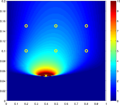
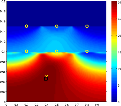
Figure 9: Identification of a single time dependent source from instantaneous measurements in one dimension with $1\%$ noise in the data. Left: forward problem solution $u(x,t)$. Right: imaging functional $\boldsymbol{J}(\boldsymbol{s})$ for $\boldsymbol{s}=(x,t)\in[0,1]\times[0,0.2]$. Horizontal axis is $x$, vertical axis is $t$. True source location is yellow $\times$, measurement locations are yellow $\circ$, source position estimated by Algorithm 1 is black $\square$. True source parameters $(a,y,\tau)$ are $(3,0.4,0.05)$, estimated are $(3.178,0.392,0.045)$.

Let us consider a scalar forward problem of the form (2.1) with $\epsilon=1$, $\boldsymbol{w}=0$, $\boldsymbol{L}=5$, $\boldsymbol{Q}(\boldsymbol{u})=-u$, $\Omega=[0,1]$ and $T=0.2$. A single source of the form

$$f(x,t)=a\delta(t-\tau)\delta(x-y)$$ (4.64)

is to be determined, where $a=3$, $\tau=0.05$ and $y=0.4$.

Similarly to the two dimensional case we use a finite difference scheme in space and an exponential integrator in time. To avoid committing an inverse crime we use a fine grid to compute the forward solution for simulating the data with $200$ grid steps in $x$ and $120$ time steps. A coarser grid is used in Algorithm 1 to identify the source with $101$ steps in both spatial and temporal variables.

We observed from our numerical experiments that identification of time dependent sources is more sensitive to noise and numerical errors than the identification of sources in examples in sections 4.3 and 4.4. Thus, for stable source identification we need to use more measurements than is required to just make the system (2.23) formally determined. The source in (4.64) is determined by three parameters, but we use six measurements for our numerical example. We make measurements at spatial locations $0.2$, $0.5$ and $0.8$ at two time instants $0.1$ and $0.15$ for a total of $6$ measurements.

The results of the forward simulation and source identification by Algorithm 1 are shown in Figure 9. We observe that both the source location and its intensity were identified reasonably well given the noisy data. The plot of the imaging functional $\boldsymbol{J}(\boldsymbol{s})$ explains why the time dependent source identification problem is more difficult than the previously considered examples. The imaging functional has a large plateau surrounding the true source location, which decreases the discriminatory power of the method. For higher noise levels we observed that the estimated source location ends up somewhere on this plateau far away from the true source position.

4.5.2 Two dimensional case

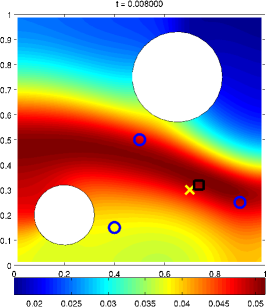
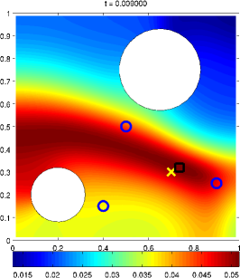
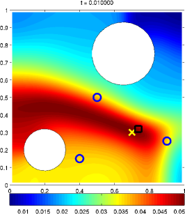
Figure 10: Identification of a single time dependent source from instantaneous measurements in two dimensions with $1\%$ noise in the data. Left to right: slices of the imaging functional $J(\boldsymbol{s})$, $\boldsymbol{s}=(\boldsymbol{y},t)$ for the three values of $t=0.008,0.009,0.010$ and $\boldsymbol{y}\in\Omega$. True source spatial location is yellow $\times$, measurement spatial locations are blue $\circ$. Source spatial position estimated by Algorithm 1 is black $\square$. True source parameters $(a,x,y,\tau)$ are $(10,0.7,0.3,0.010)$, estimated are $(11.18,0.73,0.31,0.009)$.

Here we present the results of time dependent source identification for the three component chemical system in two dimensions from instantaneous measurements. As we observed in Section 4.5.1 such source detection is more difficult than the cases considered in sections 4.3 and 4.4, so for stable identification we reduced the non-linearity of the system by taking smaller reaction rates $k_{1}=100$ and $k_{2}=200$. Higher reaction rates leading to stiffer system can be handled using more efficient numerical schemes, for example [8]. However, proper numerical treatment of stiff systems is out of the scope of this work, so for convenience we work with reduced reaction rates in this section.

We simulate the system up to $T=0.03$, which is the time when the system is still in transient behavior. The source goes off at $\tau=0.01$ and we make two sets of three point measurements each at instants $\theta=0.015$ and $\theta=0.020$ for a total of six measurements.

In Figure 10 we show three slices of the imaging functional $J(\boldsymbol{s})$ at time instants adjacent to the temporal source location estimated by Algorithm 1. We observe that the imaging functional has a narrow ridge with a plateau on top, which can make source identification difficult similarly to the one dimensional case, where in the presence of noise Algorithm 1 can get stuck far away from the true source location.

5 Conclusions and future work

We presented here a method for source identification in non-linear time dependent advection-diffusion-reaction systems. We also provided the results of extensive numerical experiments that suggest that our method performs well in the presence of noise in the data and/or uncertainty in the number of sources present. The numerical experiments also show that the method’s performance can be further improved by adaptively adding more measurements using the proposed strategy.

The following topics of future study can be proposed. First, determining the conditions under which Algorithm 1 converges and proving the convergence. The analysis is complicated by the lack of regularity of solutions in the presence of point sources and by the coupling between the forward iteration and source estimation at each step of the algorithm.

Second, the study of the case where only a partial knowledge of domain $\Omega$ is assumed. In this case both the sources and the obstacles need to be determined. A method proposed in [3] solves the linear case by using the comparison results for elliptic equations. Since similar results hold for non-linear parabolic systems, it should be possible to extend the method in [3] to the setting considered here.

Third, in this paper we assumed that all system parameters such as reaction rates, advection field and diffusion coefficients are known. In reality these parameters are estimated from some other measurements and thus are prone to inaccuracies. One may study the sensitivity of source identification with respect to uncertainties in the system parameters, or even try to estimate these parameters as a part of the source identification problem.

References

References

- [1] V. Akcelik, G. Biros, A. Draganescu, O. Ghattas, J. Hill, and B. van Bloemen Waanders. Inversion of airborne contaminants in a regional model. Computational Science–ICCS 2006, 3993/2006:481–488, 2006.
- [2] A.H. Al-Mohy and N.J. Higham. Computing the action of the matrix exponential, with an application to exponential integrators. SIAM journal on scientific computing, 33(2):488–511, 2011.
- [3] M. Burger, Y. Landa, N. Tanushev, and R. Tsai. Discovering a point source in unknown environments. Algorithmic Foundation of Robotics VIII, pages 663–678, 2009.
- [4] E.J. Candes, J. Romberg, and T. Tao. Robust uncertainty principles: Exact signal reconstruction from highly incomplete frequency information. Information Theory, IEEE Transactions on, 52(2):489–509, 2006.
- [5] E.J. Candes, J.K. Romberg, and T. Tao. Stable signal recovery from incomplete and inaccurate measurements. Communications on pure and applied mathematics, 59(8):1207–1223, 2006.
- [6] P. Ciais, P. Rayner, F. Chevallier, P. Bousquet, M. Logan, P. Peylin, and M. Ramonet. Atmospheric inversions for estimating CO2 fluxes: methods and perspectives. Climatic Change, 103:69–92, 2010.
- [7] D.L. Colton and R. Kress. Inverse acoustic and electromagnetic scattering theory, volume 93. Springer, 1998.
- [8] B. Engquist and Y.H. Tsai. Heterogeneous multiscale methods for stiff ordinary differential equations. Mathematics of computation, 74(252):1707–1742, 2005.
- [9] I.G. Enting. Inverse Problems in Atmospheric Constituent Transport. Cambridge Atmospheric and Space Science Series. Cambridge University Press, 2002.
- [10] B. Farmer, C. Hall, and S. Esedoglu. Source identification from line integral measurements and simple atmospheric models. Preprint, 2011.
- [11] E. Haber, L. Horesh, and L. Tenorio. Numerical methods for experimental design of large-scale linear ill-posed inverse problems. Inverse Problems, 24:055012, 2008.
- [12] M.Z. Jacobson. Fundamentals of atmospheric modeling. Cambridge University Press, 2005.
- [13] S. Kamin and LA Peletier. Singular solutions of the heat equation with absorption. In Proc. Am. Math. Soc, volume 95, pages 205–210, 1985.
- [14] S. Kamin and LA Peletier. Source-type solutions of degenerate diffusion equations with absorption. Israel journal of mathematics, 50(3):219–230, 1985.
- [15] P.S. Kasibhatla and American Geophysical Union. Inverse methods in global biogeochemical cycles. Number v. 1 in Geophysical monograph. American Geophysical Union, 2000.
- [16] J. Kim and S.Y. Cho. Computation accuracy and efficiency of the time-splitting method in solving atmospheric transport/chemistry equations. Atmospheric Environment, 31(15):2215–2224, 1997.
- [17] Y. Li, S. Osher, and R. Tsai. Heat source identification based on l1 constrained minimization. UCLA CAM report 11-04, 2011.
- [18] F. Pukelsheim. Optimal design of experiments, volume 50. Society for Industrial Mathematics, 2006.
- [19] J. Smoller. Shock waves and reaction-diffusion equations. Springer, 1994.
- [20] B. Sportisse. An analysis of operator splitting techniques in the stiff case. Journal of Computational Physics, 161(1):140–168, 2000.
- [21] W. Yin, S. Osher, D. Goldfarb, and J. Darbon. Bregman iterative algorithms for l1-minimization with applications to compressed sensing. SIAM J. Imaging Sci, 1(1):143–168, 2008.