QED calculation of the nuclear magnetic shielding for hydrogen-like ions

Abstract

We report an ab initio calculation of the shielding of the nuclear magnetic moment by the bound electron in hydrogen-like ions. This investigation takes into account several effects that have not been calculated before (electron self-energy, vacuum polarization, nuclear magnetization distribution), thus bringing the theory to the point where further progress is impeded by the uncertainty due to nuclear-structure effects. The QED corrections are calculated to all orders in the nuclear binding strength parameter and, independently, to the leading order in the expansion in this parameter. The results obtained lay the ground for the high-precision determination of nuclear magnetic dipole moments from measurements of the $g$-factor of hydrogen-like ions.

I Introduction

Last years showed much progress in the experimental determination of the $g$-factors of hydrogen-like ions haeffner:00:prl ; verdu:04 ; sturm:11 ; sturm:11:b . Measurements, accurate up to a few parts in $10^{11}$ sturm:11:b , were performed by studying a single ion confined in a Penning trap. These experiments provided the stringent tests of bound-state quantum electrodynamics (QED) theory and yielded the best determination of the electron mass mohr:08:rmp .

In order to match the experimental accuracy, many sophisticated calculations were performed during the past years, in particular those of the one-loop self-energy blundell:97:pra ; persson:97:g ; yerokhin:02:prl , the one-loop vacuum-polarization karshenboim:02:plb , the nuclear recoil shabaev:02:recprl , and the two-loop QED effects pachucki:04:prl ; pachucki:05:gfact . These calculations made it possible to determine the electron mass from the experimental values of the bound-electron $g$ factor beier:02:prl . The theoretical accuracy of the bound-electron $g$ factor in hydrogen-like ions is presently at the $10^{-11}$ level pachucki:05:gfact for light elements up to carbon but deteriorates quickly for heavier elements because of the unknown higher-order two-loop QED effects scaling with the nuclear charge number $Z$ as $Z^{5}$.

The experimental investigations of the $g$-factors of hydrogen-like ions were so far performed for ions with spinless nuclei. However, when applied to the ions with a non-zero nuclear spin, such investigations can be useful as a new method for the determination of the magnetic dipole moments of the nuclei. This method has important advantages over the more traditional approaches, such as nuclear magnetic resonance (NMR), atomic beam magnetic resonance, collinear laser spectroscopy, and optical pumping (OP). These advantages are that (i) the simplicity of the system under investigation (a hydrogen-like ion) allows for an ab initio theoretical description with a reliable estimation of uncalculated effects and (ii) the influence of the nuclear-structure effects (which are the main limiting factors for theory) is relatively weak. This is in contrast to the existing methods, in which the experimental data should be corrected for several physical effects, which are difficult to calculate. Among such effects is the diamagnetic shielding of the external magnetic field by the electrons in the atom. The NMR results should be also corrected for the paramagnetic chemical shift caused by the chemical environment ramsey:50:dia and the OP data are sensitive to the hyperfine mixing of the energy levels lahaye:70 . Significant (and generally unknown) uncertainties of calculations of these effects often lead to ambiguities in the published values of nuclear magnetic moments gustavsson:98:pra .

The goal of the present investigation is to perform an ab initio calculation of the $g$-factor of a hydrogen-like ion with a non-zero nuclear spin. It can be demonstrated that the nuclear-spin dependent part of the atomic $g$-factor can be parameterized in terms of the nuclear magnetic shielding constant $\sigma$, which describes the effective reduction of the coupling of the nuclear magnetic moment $\vec{\mu}$ to an external magnetic field $\vec{B}$ caused by the shell electron(s),

$$-\vec{\mu}\cdot\vec{B}\to-\vec{\mu}\cdot\vec{B}\,(1-\sigma)\,.$$ (1)

The relativistic theory of the $g$-factor of a hydrogen-like ion with a non-zero nuclear spin (and, thus, the theory of the nuclear magnetic shielding) was examined in detail in Ref. moskovkin:04 . In the present work, we go beyond the relativistic description of the nuclear magnetic shielding and calculate the dominant corrections to it, namely, the self-energy, the vacuum-polarization, and the nuclear magnetization distribution corrections. As a result, we bring the theory to the point where the uncertainty due to nuclear-structure effects impedes further progress.

The main challenge of the present work is the calculation of the self-energy correction. To the best of our knowledge, the only previous attempt to address it was made in Ref. rudzinski:09 . In that work, the self-energy contribution to the shielding constant was estimated by the leading logarithm of its ${Z\alpha}$ expansion (where $\alpha$ is the fine-structure constant). In our work, we calculate the self-energy correction rigorously to all orders in the binding nuclear strength parameter ${Z\alpha}$ and, independently, perform an analytical calculation to the leading order in the expansion in this parameter (including both the logarithm and constant terms). First results of this work were reported in Ref. yerokhin:11:prl .

The rest of the paper is organized as follows. In Sec. II we summarize the relativistic theory of the $g$-factor of an ion with a non-zero nuclear spin and the theory of the nuclear magnetic shielding. Our calculation of the self-energy and vacuum-polarization corrections to all orders in ${Z\alpha}$ is described in Sec. III. In Sec. IV we report the calculation of the QED correction to the nuclear magnetic shielding to the leading order in the ${Z\alpha}$ expansion. Sec. V deals with the other effects, namely, the nuclear magnetization distribution, the nuclear recoil, and the quadrupole interaction. Numerical results and discussion are given in Sec. VI. The paper ends with conclusion in Sec. VII.

The relativistic units ($m$ = $\hbar=c=1$) and the charge units $\alpha=e^{2}/(4\pi)$ are used throughout this paper.

II Leading-order magnetic shielding

We consider a hydrogen-like ion with a non-zero spin nucleus placed in a weak homogenous magnetic field $\vec{B}$ directed along the $z$ axis. Assuming that the energy shift due to the interaction with the $\vec{B}$ field (the Zeeman shift) is much smaller than the hyperfine-structure splitting (hfs), the energy shift can be expressed in terms of the $g$ factor of the atomic system $g_{F}$,

$$\Delta E=g_{F}\,\mu_{0}\,B\,M_{F}\,,$$ (2)

where $B=|\vec{B}|$, $\mu_{0}=|e|/(2m)$ is the Bohr magneton, $e$ and $m$ are the elementary charge and the electron mass, respectively, and $M_{F}$ is the $z$ projection of the total angular momentum of the system $F$. To the leading order, the energy shift is given by

$$\Delta E=\langle FM_{F}|\left[-\frac{e}{2}\,(\vec{r}\times\vec{\alpha})\cdot\vec{B}-\vec{\mu}\cdot\vec{B}\right]|FM_{F}\rangle\,,$$ (3)

where $|FM_{F}\rangle\equiv|jIFM_{F}\rangle$ is the wave function of the ion, $j$ and $I$ are the angular momentum quantum numbers of the electron and nucleus, respectively; $\vec{\mu}$ is the operator of the magnetic moment of the nucleus. The matrix element (3) can easily be evaluated, yielding the well-known leading-order relativistic result bethesalpeter ,

$$g^{(0)}_{F}=g_{j}^{(0)}\,\frac{\langle\vec{j}\cdot\vec{F}\rangle}{F(F+1)}-\frac{m}{m_{p}}\,g_{I}\,\frac{\langle\vec{I}\cdot\vec{F}\rangle}{F(F+1)}\,,$$ (4)

where $g_{j}^{(0)}$ is the Dirac bound-electron $g$ factor breit:28 , $g_{I}=\mu/(\mu_{N}I)$ is the nuclear $g$ factor, $\mu=\langle II|\vec{\mu}|II\rangle$ is the nuclear magnetic moment, $\mu_{N}=|e|/(2m_{p})$ is the nuclear magneton, $m_{p}$ is the proton mass, and $\langle\vec{j}\cdot\vec{F}\rangle$ and $\langle\vec{I}\cdot\vec{F}\rangle$ are the angular-momentum recoupling coefficients,

$$\langle\vec{j}\cdot\vec{F}\rangle = [F(F+1)-I(I+1)+j(j+1)]/2\,,$$ (5)

$$\langle\vec{I}\cdot\vec{F}\rangle = [F(F+1)+I(I+1)-j(j+1)]/2\,.$$ (6)

Generalizing the leading-order result to include the higher-order correction, we write the atomic $g$ factor $g_{F}$ as

$$g_{F}=g_{j}\,\frac{\langle\vec{j}\cdot\vec{F}\rangle}{F(F+1)}-\frac{m}{m_{p}}\,g_{I}\,(1-\sigma)\,\frac{\langle\vec{I}\cdot\vec{F}\rangle}{F(F+1)}\,.$$ (7)

In the above equation, the bound-electron $g$ factor $g_{j}=g_{j}^{(0)}+\alpha/(2\pi)+\ldots$ incorporates all corrections that do not depend on the nuclear spin, whereas the nuclear shielding constant $\sigma$ parameterizes the nuclear-spin dependent corrections. The bound-electron $g$ factor $g_{j}$ has been extensively studied during the last years, both theoretically yerokhin:02:prl ; karshenboim:02:plb ; shabaev:02:recprl ; pachucki:04:prl ; pachucki:05:gfact and experimentally haeffner:00:prl ; verdu:04 ; sturm:11 . The goal of the present work is the ab initio theoretical description of the nuclear shielding parameter $\sigma$.

It can be seen from Eq. (7) that the nuclear-spin dependent contribution to the atomic $g$ factor $g_{F}$ is suppressed by the electron-to-proton mass ratio and thus is by about three orders of magnitude smaller than the nuclear-spin independent part proportional to $g_{j}$. It is, however, possible to form a combination of the atomic $g$ factors which is free of the nuclear-spin independent contributions. So, for ions with the nuclear spin $I>\nicefrac{{1}}{{2}}$, we introduce the sum of the atomic $g$ factors $\overline{g}$ that is directly proportional to the nuclear magnetic moment,

$$\overline{g}\equiv g_{F=I+\nicefrac{{1}}{{2}}}+g_{F=I-\nicefrac{{1}}{{2}}}=-2\frac{m}{m_{p}}\frac{\mu}{\mu_{N}I}\,(1-\sigma)\,.$$ (8)

This combination of the $g$ factors is particularly convenient for the determination of the nuclear magnetic dipole moments from experiment. Indeed, if both the $g_{F=I+\nicefrac{{1}}{{2}}}$ and $g_{F=I-\nicefrac{{1}}{{2}}}$ $g$-factors are measured and $\sigma$ is known from theory, Eq. (8) determines the nuclear magnetic moment $\mu$. For the ions with a nuclear spin $I=\nicefrac{{1}}{{2}}$, Eq. (8) is not applicable and the nuclear magnetic moment should be determined from Eq. (7).

Contributions to the nuclear magnetic shielding are described by Feynman diagrams with two external interactions, one with the external magnetic field (the Zeeman interaction),

$$V_{\rm zee}(r)=\frac{|e|}{2}\,\vec{B}\cdot(\vec{r}\times\vec{\alpha})\,,$$ (9)

and another, with the magnetic dipole field of the nucleus (the hfs interaction)

$$V_{\rm hfs}(r)=\frac{|e|}{4\pi}\,\vec{\mu}\cdot\frac{\vec{r}\times\vec{\alpha}}{r^{3}}\,.$$ (10)

The leading-order contribution to the magnetic shielding comes from the following energy shift

$$\Delta E=2\,\sum_{n\neq a}\frac{1}{\varepsilon_{a}-\varepsilon_{n}}\langle a|V_{\rm zee}|n\rangle\langle n|V_{\rm hfs}|a\rangle\,,$$ (11)

where the summation runs over the whole Dirac spectrum with the reference state excluded. As follows from Eqs. (2) and (7), contributions to the shielding constant $\delta\sigma$ are obtained from the corresponding energy shifts $\delta E$ by

$$\delta\sigma=\frac{\delta E}{\mu\,B\,M_{F}\,\frac{\langle\vec{I}\cdot\vec{F}\rangle}{IF(F+1)}}\,.$$ (12)

For the electronic states with $j_{a}=1/2$, all nuclear quantum numbers in Eq. (11) can be factorized out. The expression for the shielding constant is then obtained from that formula by using the following substitutions

$$V_{\rm zee}\to\widetilde{V}_{\rm zee}\equiv(\vec{r}\times\vec{\alpha})_{0}\,,\ \ \ V_{\rm hfs}\to\widetilde{V}_{\rm hfs}\equiv\frac{\displaystyle(\vec{r}\times\vec{\alpha})_{0}}{\displaystyle r^{3}}\,,\ \ \$$

$$|a\rangle\to|a_{\nicefrac{{1}}{{2}}}\rangle\,,\ \ \ |n\rangle\to|n_{\nicefrac{{1}}{{2}}}\rangle\,,$$

$$2\to\alpha\ \ \mbox{\rm(prefactor)}\,,$$ (13)

where the zero subscript refers to the zero spherical component of the vector. Here and in what follows, $|n_{\nicefrac{{1}}{{2}}}\rangle\equiv|\kappa_{n},\mu_{n}=\nicefrac{{1}}{{2}}\rangle$ denotes the Dirac state with the relativistic angular quantum number $\kappa_{n}$ and the fixed momentum projection $\mu_{n}=1/2$.

So, for $j_{a}=1/2$, the leading contribution to the magnetic shielding is given by a simple expression

$$\sigma^{(0)}= \,\alpha\sum_{n\neq a}\frac{1}{\varepsilon_{a}-\varepsilon_{n}}\,\langle a_{\nicefrac{{1}}{{2}}}|\widetilde{V}_{\rm zee}|n_{\nicefrac{{1}}{{2}}}\rangle\langle n_{\nicefrac{{1}}{{2}}}|\widetilde{V}_{\rm hfs}|a_{\nicefrac{{1}}{{2}}}\rangle\,.$$ (14)

Performing the angular integrations with help of Eq. (129), one gets for the $ns$ reference state

$$\sigma^{(0)}=\alpha\sum_{\kappa_{n}=-1,2}x_{\kappa_{n}}^{2}\,\sum_{n\neq a}\frac{R_{an}^{(1)}\,R_{na}^{(-2)}}{\varepsilon_{a}-\varepsilon_{n}}\,,$$ (15)

where $R^{(\alpha)}$ are the radial integrals of the form

$$R^{(\alpha)}_{ab}=\int_{0}^{\infty}dr\,r^{2+\alpha}\bigl{[}g_{a}(r)f_{b}(r)+f_{a}(r)g_{b}(r)\bigr{]}\,,$$ (16)

$g(r)$ and $f(r)$ are the upper and lower radial components of the Dirac wave function, respectively, and the angular prefactors $x_{\kappa_{n}}$ are given by $x_{\kappa_{n}=-1}=-2/3$, $x_{\kappa_{n}=2}=-\sqrt{2}/3$.

For the point nuclear model, the sum over the Dirac spectrum in the above expression can be evaluated analytically moore:99 ; pyper:99:a ; pyper:99:b , see also more recent studies moskovkin:04 ; ivanov:09 ,

$$\sigma^{(0)} = -\frac{4\alpha{Z\alpha}}{9}\left(\frac{1}{3}-\frac{1}{6(1+\gamma)}+\frac{2}{\gamma}-\frac{3}{2\gamma-1}\right)$$ (17)

$$= \alpha{Z\alpha}\left(\frac{1}{3}+\frac{97}{108}({Z\alpha})^{2}+\ldots\right)\,,$$

where $\gamma=\sqrt{1-({Z\alpha})^{2}}$. For the extended nucleus, the calculation is easily performed numerically moskovkin:04 .

III QED correction

Figure 1: Self-energy correction to the nuclear magnetic shielding. Double line represents the electron in the binding nuclear field. The wave line terminated by a triangle represents the dipole hyperfine interaction with the nucleus and the wave line terminated by a cross represents the interaction with the external magnetic field.

III.1 Self-energy: General formulas

The self-energy correction in the presence of the external magnetic field and the magnetic dipole field of the nucleus is graphically represented by six topologically non-equivalent Feynman diagrams shown in Fig. 1. General expressions for these diagrams are conveniently obtained by using the two-time Green’s function method shabaev:02:rep . The resulting formulas are summarized below.

III.1.1 Perturbed-orbital contribution

The irreducible contributions of diagrams on Figs. 1(a)-(c) can be represented in terms of the one-loop self-energy operator $\Sigma$. This part will be termed as the perturbed-orbital contribution. The corresponding energy shift is

$$\Delta E_{\rm po} = 2\,\langle\Sigma_{R}\,\frac{1}{(\varepsilon_{a}-H)^{\prime}}\,V_{\rm zee}\,\frac{1}{(\varepsilon_{a}-H)^{\prime}}\,V_{\rm hfs}\rangle$$

$$+2\,\langle\Sigma_{R}\,\frac{1}{(\varepsilon_{a}-H)^{\prime}}\,V_{\rm hfs}\,\frac{1}{(\varepsilon_{a}-H)^{\prime}}\,V_{\rm zee}\rangle$$

$$-2\,\langle\Sigma_{R}\,\frac{1}{(\varepsilon_{a}-H)^{2^{\prime}}}\,V_{\rm zee}\rangle\langle V_{\rm hfs}\rangle$$

$$-2\,\langle\Sigma_{R}\,\frac{1}{(\varepsilon_{a}-H)^{2^{\prime}}}\,V_{\rm hfs}\rangle\langle V_{\rm zee}\rangle$$

$$-2\,\langle\Sigma_{R}\rangle\langle V_{\rm zee}\,\frac{1}{(\varepsilon_{a}-H)^{2^{\prime}}}\,V_{\rm hfs}\rangle$$

$$+2\,\langle V_{\rm zee}\,\frac{1}{(\varepsilon_{a}-H)^{\prime}}\,\Sigma_{R}\,\frac{1}{(\varepsilon_{a}-H)^{\prime}}\,V_{\rm hfs}\rangle\,,$$

where we used the short-hand notations for the reduced Green’s function,

$$\frac{1}{(\varepsilon_{a}-H)^{{\prime}}}=\sum_{n\neq a}\frac{|n\rangle\langle n|}{\varepsilon_{a}-\varepsilon_{n}}\,,$$ (19)

and its derivative

$$\frac{1}{(\varepsilon_{a}-H)^{2^{\prime}}}=\sum_{n\neq a}\frac{|n\rangle\langle n|}{(\varepsilon_{a}-\varepsilon_{n})^{2}}\,.$$ (20)

The (unrenormalized) self-energy operator $\Sigma(\varepsilon)$ is defined by its matrix elements as follows

$$\langle i|\Sigma(\varepsilon)|k\rangle = \frac{i}{2\pi}\int_{-\infty}^{\infty}d\omega\sum_{n}\frac{\langle in|I(\omega)|nk\rangle}{\varepsilon-\omega-u\,\varepsilon_{n}}\,,$$ (21)

where $I(\omega)$ is the operator of the electron-electron interaction, $I(\omega)=e^{2}\alpha_{\mu}\alpha_{\nu}D^{\mu\nu}(\omega)$, $D^{\mu\nu}(\omega)$ is the photon propagator, $\alpha_{\mu}$ are the Dirac matrices, and $u\equiv 1-i0$, where $i0$ is a small imaginary addition that defines the positions of the poles of the electron propagators with respect to the integration contour. The summation over $n$ runs over the complete Dirac spectrum. Renormalization of the one-loop self-energy operator is well described in the literature, see, e.g., Ref. snyderman:91 . In this work, the renormalized part of the self-energy operator is defined as

$$\Sigma_{R}(\varepsilon)=\Sigma(\varepsilon)-\beta\,\delta m-(\varepsilon-\vec{\alpha}\cdot\vec{p}-\,V_{C}-\beta m)\,B^{(1)}\,,$$ (22)

where $\delta m$ is the mass counterterm, $\beta$ is the Dirac $\beta$ matrix, $B^{(1)}$ is the one-loop renormalization constant, $V_{C}$ is the binding Coulomb potential of the nucleus, and the renormalization is to be performed in momentum space with a covariant regularization of ultraviolet (UV) divergencies. Details on the renormalization procedure and explicit formulas for $\Sigma_{R}(\varepsilon)$ can be found in Refs. yerokhin:99:pra ; yerokhin:03:epjd .

III.1.2 Single-vertex contributions

The irreducible contribution of the diagram shown in Fig. 1(d), together with the corresponding derivative term, is referred to as the hfs-vertex contribution. It is given by

$$\Delta E_{\rm vr,hfs} = 2\,\langle\Gamma_{{\rm hfs},R}\,\frac{1}{(\varepsilon_{a}-H)^{{\prime}}}\,V_{\rm zee}\rangle$$ (23)

$$+2\,\langle\Sigma^{\prime}_{R}\,\frac{1}{(\varepsilon_{a}-H)^{{\prime}}}\,V_{\rm zee}\rangle\,\langle V_{\rm hfs}\rangle\,,$$

where $\Gamma_{{\rm hfs},R}\equiv\Gamma_{{\rm hfs},R}(\varepsilon_{a})$ is the renormalized part of the 3-point vertex representing the interaction with the hfs field and $\Sigma^{\prime}_{R}\equiv\Sigma^{\prime}_{R}(\varepsilon_{a})$ is the derivative of the renormalized self-energy operator over the energy argument, $\Sigma^{\prime}_{R}(\varepsilon_{a})=\left.d/(d\varepsilon)\Sigma_{R}(\varepsilon)\right|_{\varepsilon=\varepsilon_{a}}$. The unrenormalized 3-point hfs vertex operator is defined by its matrix elements as

$$\langle i|\Gamma_{\rm hfs}(\varepsilon)|k\rangle \ =\frac{i}{2\pi}\int_{-\infty}^{\infty}d\omega$$

$$\times\sum_{n_{1}n_{2}}\frac{\langle in_{2}|I(\omega)|n_{1}k\rangle\langle n_{1}|V_{\rm hfs}|n_{2}\rangle}{(\varepsilon-\omega-u\varepsilon_{n_{1}})(\varepsilon-\omega-u\varepsilon_{n_{2}})}\,.$$ (24)

The renormalized part of the operator is obtained as

$$\Gamma_{{\rm hfs},R}(\varepsilon)=\Gamma_{{\rm hfs}}(\varepsilon)-V_{\rm hfs}\,L^{(1)}\,,$$ (25)

where $L^{(1)}$ is the one-loop renormalization constant and the renormalization is to be performed in momentum space with a covariant regularization of UV divergencies, see Ref. yerokhin:03:epjd for details.

The irreducible contribution of the diagram shown in Fig. 1(e), together with the corresponding derivative term, is referred to as the Zeeman-vertex contribution. It is given by

$$\Delta E_{\rm vr,zee} = 2\,\langle\Gamma_{{\rm zee},R}\,\frac{1}{(\varepsilon_{a}-H)^{{\prime}}}\,V_{\rm hfs}\rangle$$ (26)

$$+2\,\langle\Sigma^{\prime}_{R}\,\frac{1}{(\varepsilon_{a}-H)^{{\prime}}}\,V_{\rm hfs}\rangle\,\langle V_{\rm zee}\rangle\,,$$

where the 3-point Zeeman vertex is defined analogously to the hfs one.

III.1.3 Double-vertex contribution

The contribution of the diagram shown on Fig. 1(f), together with the corresponding derivative terms, will be termed as the double-vertex contribution. It is defined by

$$\Delta E_{\rm d.vr}=2\,\langle\Lambda(\varepsilon_{a})\rangle$$

$$+\langle\Sigma^{\prime\prime}\rangle\langle V_{\rm zee}\rangle\langle V_{\rm hfs}\rangle+\langle\Gamma_{\rm hfs}^{\prime}\rangle\langle V_{\rm zee}\rangle+\langle\Gamma_{\rm zee}^{\prime}\rangle\langle V_{\rm hfs}\rangle$$

$$-2\,\langle V_{\rm zee}\frac{1}{(\varepsilon_{a}-H)^{\prime}}V_{\rm hfs}\rangle\,\frac{i}{2\pi}\int_{-\infty}^{\infty}d\omega\sum_{a^{\prime}}\frac{\langle aa^{\prime}|I(\omega)|a^{\prime}a\rangle}{(-\omega+i0)^{2}}\,,$$ (27)

where $\Lambda$ denotes the 4-point vertex representing the interaction with both the Zeeman and hfs interactions,

$$\langle i|\Lambda(\varepsilon)|k\rangle=\frac{i}{2\pi}\int_{-\infty}^{\infty}d\omega$$

$$\times\sum_{n_{1}n_{2}n_{3}}\frac{\langle in_{3}|I(\omega)|n_{1}k\rangle\langle n_{1}|V_{\rm zee}|n_{2}\rangle\langle n_{2}|V_{\rm hfs}|n_{3}\rangle}{(\varepsilon-\omega-u\varepsilon_{n_{1}})(\varepsilon-\omega-u\varepsilon_{n_{2}})(\varepsilon-\omega-u\varepsilon_{n_{3}})}\,,$$ (28)

$\Sigma^{\prime\prime}\equiv\Sigma^{\prime\prime}(\varepsilon_{a})$ denotes the second derivative of the self-energy operator over the energy argument, $\Sigma^{\prime\prime}(\varepsilon_{a})=\left.d^{2}/(d^{2}\varepsilon)\,\Sigma(\varepsilon)\right|_{\varepsilon=\varepsilon_{a}}$, $\Gamma^{\prime}\equiv\Gamma^{\prime}(\varepsilon_{a})$ denotes the derivative of the vertex operator over the energy argument, and $a^{\prime}$ denotes the intermediate electron states with the energy $\varepsilon_{a^{\prime}}=\varepsilon_{a}$. The last term in Eq. (III.1.3) is added artifically, in order to make the whole expression for $\Delta E_{\rm d.vr}$ infrared (IR) finite. The same term will be subtracted from the derivative contribution defined below, see Eq. (29).

We note that all terms in Eq. (III.1.3) are UV finite, so that there is no need for any UV regularization. There are, however, IR divergences, which appear when the energy of the intermediate electron states in the electron propagators coincides with the energy of the reference state. The divergences cancel out in the sum of individual terms in Eq. (III.1.3).

III.1.4 Derivative contribution

Finally, the remaining contribution will be termed as the derivative term. It is given by

$$\Delta E_{\rm der} = 2\,\biggl{[}\langle\Sigma^{\prime}_{R}\rangle+\frac{i}{2\pi}\int_{-\infty}^{\infty}d\omega\sum_{a^{\prime}}\frac{\langle aa^{\prime}|I(\omega)|a^{\prime}a\rangle}{(-\omega+i0)^{2}}\biggr{]}$$ (29)

$$\times\langle V_{\rm zee}\,\frac{1}{(\varepsilon_{a}-H)^{{\prime}}}\,V_{\rm hfs}\rangle\,.$$

The second term in the brackets is added artifically, in order to compensate the IR reference-state divergence present in the first term, making the total expression for $\Delta E_{\rm der}$ IR finite. Note that this term is exactly the same as the one added to Eq. (III.1.3) but has the opposite sign.

Finally, the total self-energy correction is given by the sum of the contributions discussed above,

$$\Delta E_{\rm SE}=\Delta E_{\rm po}+\Delta E_{\rm vr,hfs}+\Delta E_{\rm vr,zee}+\Delta E_{\rm d.vr}+\Delta E_{\rm der}\,,$$ (30)

which are given by Eqs. (III.1.1), (23), (26), (III.1.3), and (29), respectively.

III.2 Self-energy: Calculation

The general formulas reported so far represent contributions to the energy shift. We now have to separate out the nuclear degrees of freedom and convert the corrections to the energy into corrections to the shielding constant. In most cases, this is achieved simply by using the substitutions (II). The double-vertex contribution, however, requires an explicit angular-momentum algebra calculation for the separation of the nuclear variables.

We will see that most of the corrections to the shielding constant can be regarded as generalizations of the corrections already discussed in the literature. So, our present calculation will be largely based on the previous investigations of the self-energy correction to the Lamb shift yerokhin:99:pra ; yerokhin:05:se , to the hyperfine structure yerokhin:05:hfs ; yerokhin:08:prl ; yerokhin:10:sehfs , and to the $g$ factor yerokhin:04 ; yerokhin:08:prl ; yerokhin:10:sehfs . The double-vertex correction of the kind similar to that in the present work appeared in the evaluation of the self-energy correction to the parity-nonconserving transitions in Refs. shabaev:05:prl ; shabaev:05:pra . However, in this work we develop a different scheme for the evaluation of the double-vertex contribution based on the analytical representation of the Dirac-Coulomb Green function.

III.2.1 Perturbed-orbital contributions

The matrix elements of the self-energy operator are diagonal in the relativistic angular momentum quantum number $\kappa$ and the momentum projection $\mu$. Because of this, the angular reduction of the perturbed-orbital contribution is achieved by the same set of substitutions (II) as for the leading-order magnetic shielding. The resulting contribution to the shielding constant is conveniently represented as

$$\Delta\sigma_{\rm po} = \alpha\,\langle a_{\nicefrac{{1}}{{2}}}|\Sigma_{R}(\varepsilon_{a})|\delta^{(2)}a_{\nicefrac{{1}}{{2}}}\rangle$$ (31)

$$+\alpha\,\langle\delta^{(1)}_{\rm hfs}a_{\nicefrac{{1}}{{2}}}|\Sigma_{R}(\varepsilon_{a})|\delta^{(1)}_{\rm zee}a_{\nicefrac{{1}}{{2}}}\rangle\,,$$

where the first-order perturbations of the reference-state wave function are given by

$$|\delta^{(1)}_{\rm hfs}a_{\nicefrac{{1}}{{2}}}\rangle=\sum_{n\neq a}|n_{\nicefrac{{1}}{{2}}}\rangle\frac{1}{\varepsilon_{a}-\varepsilon_{n}}\,\langle n_{\nicefrac{{1}}{{2}}}|\widetilde{V}_{\rm hfs}|a_{\nicefrac{{1}}{{2}}}\rangle\,,$$ (32)

and

$$|\delta^{(1)}_{\rm zee}a_{\nicefrac{{1}}{{2}}}\rangle=\sum_{n\neq a}|n_{\nicefrac{{1}}{{2}}}\rangle\frac{1}{\varepsilon_{a}-\varepsilon_{n}}\,\langle n_{\nicefrac{{1}}{{2}}}|\widetilde{V}_{\rm zee}|a_{\nicefrac{{1}}{{2}}}\rangle\,,$$ (33)

and $|\delta^{(2)}a\rangle$ is the standard second-order perturbation landau:III of the reference-state wave function induced by both interactions, $\widetilde{V}_{\rm hfs}$ and $\widetilde{V}_{\rm zee}$. Note that only the diagonal in $\kappa$ part of the perturbed wave functions contributes to $\Delta\sigma_{\rm po}$. The calculation of the non-diagonal matrix elements of the self-energy operator is performed by a straightforward generalization of the method developed in Ref. yerokhin:05:se for the first-order self-energy correction to the Lamb shift.

III.2.2 Hfs-vertex contributions

The hfs-vertex correction to the energy shift (23) for the reference state with $j_{a}=\nicefrac{{1}}{{2}}$ can be converted to the correction to the magnetic shielding by the substitution (II). The result is

$$\Delta\sigma_{\rm vr,hfs}=\frac{i\alpha}{2\pi}\int_{-\infty}^{\infty}d\omega$$

$$\times\sum_{n_{1}n_{2}}\frac{\langle a_{\nicefrac{{1}}{{2}}}n_{2}|I(\omega)|n_{1}\,\delta^{(1)}_{\rm zee}a_{\nicefrac{{1}}{{2}}}\rangle\langle n_{1}|\widetilde{V}_{\rm hfs}|n_{2}\rangle}{(\varepsilon_{a}-\omega-u\,\varepsilon_{n_{1}})(\varepsilon_{a}-\omega-u\,\varepsilon_{n_{2}})}$$

$$-\langle\widetilde{V}_{\rm hfs}\rangle\,\frac{i\alpha}{2\pi}\int_{-\infty}^{\infty}d\omega\sum_{n}\frac{\langle a_{\nicefrac{{1}}{{2}}}n|I(\omega)|n\,\delta^{(1)}_{\rm zee}a_{\nicefrac{{1}}{{2}}}\rangle}{(\varepsilon_{a}-\omega-u\,\varepsilon_{n})^{2}}\,,$$ (34)

where the covariant regularization of the ultraviolet (UV) divergences is implicitly assumed. The right-hand-side of Eq. (III.2.2) differs from the vertex and reducible parts of the self-energy correction to the hyperfine structure only by the perturbed wave function $|\delta^{(1)}_{\rm zee}a\rangle$ in place of one of the reference-state wave functions $|a\rangle$. The main complication brought by this difference is that the perturbed wave function contains components with different values of the relativistic angular quantum number $\kappa$. So, for the reference state with $\kappa_{a}=-1$, the perturbed wave function has components with $\kappa=-1$ and $\kappa=2$, both of which contribute to the first term in Eq. (III.2.2), denoted in the following as $\Delta\sigma_{\rm ver,hfs}$. The second (reducible) term contains only the $\kappa=\kappa_{a}$ component of the perturbed wave function and its calculation is done exactly as described in Ref. yerokhin:05:hfs . Below, we present the generalization of formulas derived in Ref. yerokhin:05:hfs ; yerokhin:10:sehfs needed for the evaluation of $\Delta\sigma_{\rm ver,hfs}$.

As explained in Ref. yerokhin:05:hfs , the covariant separation of the UV divergences is conveniently performed by dividing the vertex contribution into the zero- and many-potential parts, according to the number of interactions with the binding Coulomb field in the electron propagator,

$$\Delta\sigma_{\rm ver,hfs}=\Delta\sigma_{\rm ver,hfs}^{(0)}+\Delta\sigma_{\rm ver,hfs}^{(1+)}\,.$$ (35)

The zero-potential part is calculated in momentum space with the dimensional regularization of the UV divergences. The Fourier transform of the $\widetilde{V}_{\rm hfs}$ is done by

$$\frac{(\vec{r}\times\vec{\alpha})_{0}}{r^{3}}\to(-4\pi i)\,\frac{(\vec{q}\times\vec{\alpha})_{0}}{\vec{q}^{2}}\,,$$ (36)

where $\vec{q}=\vec{p}_{1}-\vec{p}_{2}$ is the transferred momentum. The contribution of the zero-potential hfs vertex part to the shielding constant is

$$\Delta\sigma^{(0)}_{\rm ver,hfs} \ =-4\pi i\alpha\int\frac{d\vec{p}_{1}}{(2\pi)^{3}}\,\frac{d\vec{p}_{2}}{(2\pi)^{3}}\,$$

$$\times\overline{\psi}_{a_{\nicefrac{{1}}{{2}}}}(\vec{p}_{1})\,\frac{\left[\vec{q}\times{\vec{\Gamma}}_{R}(p_{1},p_{2})\right]_{0}}{\vec{q}^{2}}\,\psi_{\delta a_{\nicefrac{{1}}{{2}}}}(\vec{p}_{2})\,,$$ (37)

where $p_{1}$ and $p_{2}$ are 4-vectors with the fixed time component $p_{1}=(\varepsilon_{a},\vec{p}_{1})$, $p_{2}=(\varepsilon_{a},\vec{p}_{2})$, $\psi_{a}$ and $\psi_{\delta a}$ are the reference-state and the perturbed wave functions, respectively, $\overline{\psi}=\psi^{{\dagger}}\gamma^{0}$ is the Dirac conjugation, and ${\vec{\Gamma}}_{R}$ is the renormalized one-loop vertex operator yerokhin:99:pra . For evaluating the integrals over the angular variables, it is convenient to use the following representation of the vertex operator sandwiched between the Dirac wave functions

$$\overline{\psi}_{a}(\vec{p}_{1}) \ {\vec{\Gamma}}_{R}(p_{1},p_{2})\,\psi_{b}(\vec{p}_{2})=\frac{\alpha}{4\pi}\left[{\cal R}_{1}\chi^{{\dagger}}_{\kappa_{a}\mu_{a}}(\hat{\vec{p}}_{1})\,{\vec{\sigma}}\,\chi_{-\kappa_{b}\mu_{b}}(\hat{\vec{p}}_{2})\right.$$

$$+{\cal R}_{2}\chi^{{\dagger}}_{-\kappa_{a}\mu_{a}}(\hat{\vec{p}}_{1})\,{\vec{\sigma}}\,\chi_{\kappa_{b}\mu_{b}}(\hat{\vec{p}}_{2})$$

$$+({\cal R}_{3}\,\vec{p}_{1}+{\cal R}_{4}\,\vec{p}_{2})\chi^{{\dagger}}_{\kappa_{a}\mu_{a}}(\hat{\vec{p}}_{1})\chi_{\kappa_{b}\mu_{b}}(\hat{\vec{p}}_{2})$$

$$+\left.({\cal R}_{5}\,\vec{p}_{1}+{\cal R}_{6}\,\vec{p}_{2})\chi^{{\dagger}}_{-\kappa_{a}\mu_{a}}(\hat{\vec{p}}_{1})\chi_{-\kappa_{b}\mu_{b}}(\hat{\vec{p}}_{2})\right]\,,$$ (38)

where $\hat{\vec{p}}\equiv\vec{p}/|\vec{p}|$, $\chi_{\kappa\mu}(\hat{\vec{p}})$ are the spin-angular Dirac spinors rose:61 , and the scalar functions ${\cal R}_{i}$ are given by Eqs. (A7)–(A12) of Ref. yerokhin:99:sescr . Integration over the angular variables yields (cf. Eq. (30) of Ref. yerokhin:10:sehfs )

$$\Delta\sigma^{(0)}_{\rm ver,hfs} \ =-\frac{\alpha^{2}}{48\pi^{5}}\,\sum_{\kappa_{\delta a}}x_{\kappa_{\delta a}}\,i^{l_{a}-l_{\delta a}}\,\int_{0}^{\infty}dp_{1r}\,dp_{2r}\int_{|p_{1r}-p_{2r}|}^{p_{1r}+p_{2r}}dq_{r}\,\frac{p_{1r}p_{2r}}{q_{r}}\,$$

$$\times\Bigl{\{}{\cal R}_{1}\,[p_{1r}K_{1}(\kappa_{a},-\kappa_{\delta a})-p_{2r}K_{1}^{\prime}(\kappa_{a},-\kappa_{\delta a})]+{\cal R}_{2}\,[p_{1r}K_{1}(-\kappa_{a},\kappa_{\delta a})-p_{2r}K_{1}^{\prime}(-\kappa_{a},\kappa_{\delta a})]$$

$$+p_{1r}p_{2r}({\cal R}_{3}+{\cal R}_{4})\,K_{2}(\kappa_{a},\kappa_{\delta a})\,+p_{1r}p_{2r}({\cal R}_{5}+{\cal R}_{6})\,K_{2}(-\kappa_{a},-\kappa_{\delta a})\Bigr{\}}\,,$$ (39)

where $p_{i_{r}}=|\vec{p}_{i}|$, $q_{r}=|\vec{q}|$, $\kappa_{\delta a}$ is the relativistic angular quantum number of the perturbed wave function, $l_{n}=|\kappa_{n}+\nicefrac{{1}}{{2}}|-\nicefrac{{1}}{{2}}$, $x_{\kappa=-1}=-2/3$, $x_{\kappa=2}=-\sqrt{2}/3$, and the basic angular integrals $K_{i}(\kappa,\kappa^{\prime})$ are defined and evaluated in Appendix A.

The many-potential vertex contribution is free from UV divergences and thus can be calculated in coordinate space. The result after the integration over the angular variables is

$$\Delta\sigma_{\rm ver,hfs}^{(1+)} \ =\sum_{\kappa_{\delta a}=-1,2}x_{\kappa_{\delta a}}\,\frac{i\alpha^{2}}{2\pi}\int_{-\infty}^{\infty}d\omega$$

$$\times\sum_{n_{1}n_{2}}\frac{R^{(-2)}_{n_{1}n_{2}}\,\sum_{J}X_{J}(\kappa_{1},\kappa_{2})\,R_{J}(\omega,an_{2}n_{1}\delta a)}{(\varepsilon-\omega-u\,\varepsilon_{n_{1}})(\varepsilon-\omega-u\,\varepsilon_{n_{2}})}$$

$$-\ \mbox{\rm subtraction}\,,$$ (40)

where $R^{(-2)}_{n_{1}n_{2}}$ is the radial integral of the hfs type given by Eq. (16), $X_{J}$ is the angular coefficient,

$$X_{J}(\kappa_{1},\kappa_{2})= \ \frac{(-1)^{j_{\delta a}-1/2}}{\sqrt{2}}\left\{\begin{array}[]{ccc}j_{1}&j_{2}&1\\ j_{\delta a}&j_{a}&J\\ \end{array}\right\}$$ (43)

$$\times\frac{-\kappa_{1}-\kappa_{2}}{\sqrt{3}}C_{1}(-\kappa_{2},\kappa_{1})\,\,,$$ (44)

$C_{1}(\kappa_{a},\kappa_{b})$ is the reduced matrix element of the normalized spherical harmonics given by Eq. (C10) of Ref. yerokhin:99:pra , $R_{J}$ is the relativistic generalization of the Slater radial integral given by Eqs. (C1)–(C9) of Ref. yerokhin:99:pra , and the subtraction in the last line of Eq. (III.2.2) means that the contribution of the free propagators (already accounted for by the zero-potential term) needs to be subtracted.

III.2.3 Zeeman-vertex contribution

The Zeeman-vertex correction to the energy shift (26) for the reference state with $j_{a}=\nicefrac{{1}}{{2}}$ can be converted to the correction to the magnetic shielding by the substitution (II). The result has the form analogous to that for the hfs-vertex contribution,

$$\Delta\sigma_{\rm vr,zee}=\frac{i\alpha}{2\pi}\int_{-\infty}^{\infty}d\omega$$

$$\times\sum_{n_{1}n_{2}}\frac{\langle a_{\nicefrac{{1}}{{2}}}n_{2}|I(\omega)|n_{1}\,\delta^{(1)}_{\rm hfs}a_{\nicefrac{{1}}{{2}}}\rangle\langle n_{1}|\widetilde{V}_{\rm zee}|n_{2}\rangle}{(\varepsilon_{a}-\omega-u\,\varepsilon_{n_{1}})(\varepsilon_{a}-\omega-u\,\varepsilon_{n_{2}})}$$

$$-\langle\widetilde{V}_{\rm zee}\rangle\,\frac{i\alpha}{2\pi}\int_{-\infty}^{\infty}d\omega\sum_{n}\frac{\langle a_{\nicefrac{{1}}{{2}}}n|I(\omega)|n\,\delta^{(1)}_{\rm hfs}a_{\nicefrac{{1}}{{2}}}\rangle}{(\varepsilon_{a}-\omega-u\,\varepsilon_{n})^{2}}\,,$$ (45)

where the covariant regularization of the UV divergences is implicitly assumed. The above expression looks very similar to Eq. (III.2.2) and can be evaluated almost in the same way, except for the zero-potential vertex contribution. The expression for the zero-potential Zeeman vertex contribution is different from the hfs case because the momentum representation of the interaction with a constant magnetic field involves a $\delta$-function. The diagonal matrix element of the Zeeman vertex operator was evaluated previously in Ref. yerokhin:04 ; here we present the generalization of the formulas required for the non-diagonal case.

The Fourier transform of the interaction with the external magnetic field is given by

$$\vec{B}\times\vec{r}\to-i(2\pi)^{3}\,\vec{B}\times\vec{\nabla}_{\vec{p}^{\prime}}\delta^{3}(\vec{p}-\vec{p}^{\prime})\,.$$ (46)

The contribution of the zero-potential vertex to the shielding constant is

$$\Delta\sigma_{\rm ver,zee}^{(0)} = -i\alpha\int\frac{d\vec{p}\,d\vec{p}^{\prime}}{(2\pi)^{3}}\,\overline{\psi}_{a_{\nicefrac{{1}}{{2}}}}(\vec{p})$$

$$\times\left[\vec{\nabla}_{\vec{p}^{\prime}}\delta^{3}(\vec{p}-\vec{p}^{\prime})\times\vec{\Gamma}_{R}(p,p^{\prime})\right]_{0}\psi_{\delta a_{\nicefrac{{1}}{{2}}}}(\vec{p}^{\prime})\,,$$

where the gradient $\vec{\nabla}_{\vec{p}^{\prime}}$ acts on the $\delta$-function only. This expression is transformed by integrating by parts and carrying out the integration with the $\delta$-function analytically. The result after the angular integration consists of two parts (cf. Eqs. (27) and (36) of Ref. yerokhin:04 ),

$$\Delta\sigma_{\rm ver,zee}^{(0)}=\Delta\sigma_{\rm ver,zee,1}^{(0)}+\Delta\sigma_{\rm ver,zee,2}^{(0)}\,,$$ (48)

where

$$\Delta\sigma_{\rm ver,zee,1}^{(0)} \ =\frac{\alpha^{2}}{\pi}\sum_{\kappa_{\delta a}}x_{\kappa_{\delta a}}\,i^{l_{a}-l_{\delta a}}\,\int_{0}^{\infty}\frac{p^{2}dp}{8\pi^{3}}\,A(\rho)\,$$

$$\times\biggl{[}g_{a}\tilde{g}_{\delta a}\,A_{1}(\kappa_{a},\kappa_{\delta a})+f_{a}\tilde{f}_{\delta a}\,A_{1}(-\kappa_{a},-\kappa_{\delta a})$$

$$-p\,g_{a}f_{\delta a}\,A_{2}(\kappa_{a},-\kappa_{\delta a})-p\,f_{a}g_{\delta a}\,A_{2}(-\kappa_{a},\kappa_{\delta a})\biggr{]}\,,$$ (49)

and

$$\ \Delta\sigma_{\rm ver,zee,2}^{(0)}=-\frac{\alpha^{2}}{4\pi}\sum_{\kappa_{\delta a}}x_{\kappa_{\delta a}}\,i^{l_{a}-l_{\delta a}}\,\int_{0}^{\infty}\frac{p^{2}dp}{8\pi^{3}}\,$$

$$\times\biggl{\{}b_{1}(\rho)\,\bigl{[}g_{a}f^{\prime}_{\delta a}A_{2}(\kappa_{a},-\kappa_{\delta a})+f_{a}g^{\prime}_{\delta a}A_{2}(-\kappa_{a},\kappa_{\delta a})\bigr{]}$$

$$+\frac{1}{p}\,b_{1}(\rho)\,\bigl{[}g_{a}f_{\delta a}A_{3}(\kappa_{a},-\kappa_{\delta a})+f_{a}g_{\delta a}A_{3}(-\kappa_{a},\kappa_{\delta a})\bigr{]}$$

$$+b_{2}(\rho)\,\bigl{[}\tilde{g}_{a}g_{\delta a}A_{4}(\kappa_{a},\kappa_{\delta a})+\tilde{f}_{a}f_{\delta a}A_{4}(-\kappa_{a},-\kappa_{\delta a})\bigr{]}$$

$$+b_{3}(\rho)\,\bigl{[}g_{a}g_{\delta a}A_{4}(\kappa_{a},\kappa_{\delta a})-f_{a}f_{\delta a}A_{4}(-\kappa_{a},-\kappa_{\delta a})\bigr{]}\biggr{\}}\,,$$ (50)

where $\tilde{g}_{\delta a}=\varepsilon_{a}g_{\delta a}+pf_{\delta a}$, $\tilde{f}_{\delta a}=\varepsilon_{a}f_{\delta a}+pg_{\delta a}$, $\tilde{g}_{a}=\varepsilon_{a}g_{a}+pf_{a}$, $\tilde{f}_{a}=\varepsilon_{a}f_{a}+pg_{a}$, $g^{\prime}=dg(p)/dp$ and $f^{\prime}=df(p)/dp$, the scalar functions $A(\rho)$, $b_{i}(\rho)$ are given by Eqs. (24), (30)-(32) of Ref. yerokhin:04 and $A_{i}(\kappa_{1},\kappa_{2})$ are the basic angular integrals defined and evaluated in Appendix A.

Note that the expression for $\Delta\sigma_{\rm ver,zee,2}^{(0)}$ is non-symmetric with respect to $a$ and $\delta a$, but the result does not change when the two wave functions are interchanged.

III.2.4 Double-vertex contribution

The double-vertex correction is defined by Eq. (III.1.3). All parts of it are UV finite and thus can be evaluated in coordinate space. We denote the individual terms in the right-hand-side of Eq. (III.1.3) by $\delta_{i}E$ and consider each of them separately,

$$\Delta E_{\rm d.vr}=\sum_{i=1}^{5}\delta_{i}E\,.$$ (51)

The first term is

$$\delta_{1}E\equiv 2\,\langle\Lambda\rangle=2\,\frac{i}{2\pi}\int_{-\infty}^{\infty}d\omega$$

$$\times\sum_{n_{1}n_{2}n_{3}}\frac{\langle an_{3}|I(\omega)|n_{1}a\rangle\langle n_{1}|V_{\rm zee}|n_{2}\rangle\langle n_{2}|V_{\rm hfs}|n_{3}\rangle}{(\varepsilon-\omega-u\,\varepsilon_{n_{1}})(\varepsilon-\omega-u\,\varepsilon_{n_{2}})(\varepsilon-\omega-u\,\varepsilon_{n_{3}})}\,.$$ (52)

After separating the nuclear variables and integrating over the angles, the contribution to the magnetic shielding is (for $j_{a}=1/2$)

$$\delta_{1}\sigma \ =\frac{i\alpha^{2}}{2\pi}\int_{-\infty}^{\infty}d\omega\sum_{n_{1}n_{2}n_{3}}\sum_{J}X_{J}^{\rm d.ver}(\kappa_{1},\kappa_{2},\kappa_{3})\,$$

$$\times\frac{R_{J}(\omega,an_{3}n_{1}a)\,R^{(1)}_{n_{1}n_{2}}\,R^{(-2)}_{n_{2}n_{3}}}{(\varepsilon-\omega-u\,\varepsilon_{n_{1}})(\varepsilon-\omega-u\,\varepsilon_{n_{2}})(\varepsilon-\omega-u\,\varepsilon_{n_{3}})}\,,$$ (53)

where

$$X_{J}^{\rm d.ver}(\kappa_{1},\kappa_{2},\kappa_{3})=\frac{(-1)^{J+j_{a}-j_{2}}}{2}\,$$

$$\times\sum_{j_{n}=1/2,3/2}(2j_{n}+1)\left\{\begin{array}[]{ccc}1&j_{n}&j_{a}\\ J&j_{1}&j_{2}\\ \end{array}\right\}\left\{\begin{array}[]{ccc}1&j_{n}&j_{a}\\ J&j_{3}&j_{2}\\ \end{array}\right\}$$ (58)

$$\times\frac{\kappa_{1}+\kappa_{2}}{\sqrt{3}}\,C_{1}(-\kappa_{2},\kappa_{1})\,\frac{\kappa_{2}+\kappa_{3}}{\sqrt{3}}\,C_{1}(-\kappa_{3},\kappa_{2})\,.$$ (59)

Note that the expression for $\delta_{1}\sigma$ is IR divergent when any two or all three of the intermediate states have the same energy as the reference state: $\varepsilon_{n_{1}}=\varepsilon_{n_{2}}=\varepsilon_{a}$, $\varepsilon_{n_{2}}=\varepsilon_{n_{3}}=\varepsilon_{a}$, $\varepsilon_{n_{1}}=\varepsilon_{n_{3}}=\varepsilon_{a}$, $\varepsilon_{n_{1}}=\varepsilon_{n_{2}}=\varepsilon_{n_{3}}=\varepsilon_{a}$. The IR divergence cancels when all parts of Eq. (III.1.3) are added together.

The contribution of the second term to the shielding is

$$\delta_{2}\sigma \ =\frac{\alpha}{2}\,\langle\widetilde{V}_{\rm zee}\rangle\,\langle\widetilde{V}_{\rm hfs}\rangle\,\langle\Sigma^{\prime\prime}\rangle=\frac{4}{9}\,R^{(1)}_{aa}\,R^{(-2)}_{aa}\,$$

$$\times\frac{i\alpha^{2}}{2\pi}\int_{-\infty}^{\infty}d\omega\sum_{n_{1}n_{2}n_{3}}\sum_{J}\frac{(-1)^{J+j_{a}-j_{1}}}{2j_{a}+1}\,\delta_{\kappa_{1},\kappa_{2}}\,\delta_{\kappa_{1},\kappa_{3}}\,$$

$$\times\frac{R_{J}(\omega,an_{3}n_{1}a)\,N_{n_{1}n_{2}}\,N_{n_{2}n_{3}}}{(\varepsilon-\omega-u\,\varepsilon_{n_{1}})(\varepsilon-\omega-u\,\varepsilon_{n_{2}})(\varepsilon-\omega-u\,\varepsilon_{n_{3}})}\,,$$ (60)

where $N_{ab}$ is the normalization integral,

$$N_{ab}=\int_{0}^{\infty}dx\,x^{2}\,(g_{a}g_{b}+f_{a}f_{b})\,.$$ (61)

The expression for $\delta_{2}\sigma$ is IR divergent when $\varepsilon_{n_{1}}=\varepsilon_{n_{2}}=\varepsilon_{n_{3}}=\varepsilon_{a}$.

The third term is given by

$$\delta_{3}\sigma \ =\frac{1}{3}\,R_{aa}^{(1)}\,\frac{i\alpha^{2}}{2\pi}\int_{-\infty}^{\infty}d\omega\sum_{n_{1}n_{2}n_{3}}$$

$$\times\biggl{[}\frac{\sum_{J}X_{J}(\kappa_{1},\kappa_{2})\,\delta_{\kappa_{2},\kappa_{3}}\,R_{J}(\omega,an_{3}n_{1}a)\,R^{(-2)}_{n_{1}n_{2}}\,N_{n_{2}n_{3}}}{(\varepsilon-\omega-u\,\varepsilon_{n_{1}})(\varepsilon-\omega-u\,\varepsilon_{n_{2}})(\varepsilon-\omega-u\,\varepsilon_{n_{3}})}$$

$$+\frac{\sum_{J}X_{J}(\kappa_{2},\kappa_{3})\,\delta_{\kappa_{1},\kappa_{2}}\,R_{J}(\omega,an_{3}n_{1}a)\,N_{n_{1}n_{2}}\,R^{(-2)}_{n_{2}n_{3}}}{(\varepsilon-\omega-u\,\varepsilon_{n_{1}})(\varepsilon-\omega-u\,\varepsilon_{n_{2}})(\varepsilon-\omega-u\,\varepsilon_{n_{3}})}\Biggr{]}\,,$$ (62)

where

$$X_{J}(\kappa_{1},\kappa_{2})=\frac{1}{\sqrt{2}}\left\{\begin{array}[]{ccc}j_{1}&j_{2}&1\\ j_{a}&j_{a}&J\\ \end{array}\right\}\frac{-\kappa_{1}-\kappa_{2}}{\sqrt{3}}C_{1}(-\kappa_{2},\kappa_{1})\,.$$ (65)

The fourth term $\delta_{4}\sigma$ is obtained from $\delta_{3}\sigma$ by an obvious substitution $R^{(1)}\leftrightarrow R^{(-2)}$.

The fifth term is given by

$$\delta_{5}\sigma=-\sigma^{(0)}\,\frac{i\alpha}{2\pi}\int_{-\infty}^{\infty}d\omega\frac{\sum_{J}\frac{(-1)^{J}}{2j_{a}+1}\,R_{J}(\omega,aaaa)}{(-\omega+i0)^{2}}\,.$$ (66)

Finally, the total double-vertex contribution is given by the sum of the five terms discussed above,

$$\Delta\sigma_{\rm d.vr}=\sum_{i=1}^{5}\delta_{i}\sigma\,.$$ (67)

Despite the fact that the individual terms $\delta_{i}\sigma$ are IR divergent, the sum of them is finite and can be evaluated without any explicit regularization, provided that (i) the integration over the frequency of the virtual photon in the self-energy loop $\omega$ is performed after all five terms are added together and (ii) the contour of the $\omega$ integration is suitably chosen. One can show that if the $\omega$ integration is performed along the contour consisting of the low-energy and high-energy parts, as e.g., in Refs. yerokhin:05:se ; yerokhin:05:hfs , the integrand becomes regular at $\omega\to 0$ and, therefore, can be directly evaluated numerically.

The numerical evaluation of the double-vertex correction $\Delta\sigma_{\rm d.vr}$ was the most time consuming part of our calculation, due to a large number of the partial waves involved and a four-dimensional radial integration in Eq. (III.2.4). The radial integration was carried out with help of the numerical approach developed in our calculation of the two-loop self-energy and described in detail in Ref. yerokhin:03:epjd . Because of numerical cancellations between the five terms in Eq. (67), especially in the region of small values of $\omega$, we took care to treat all five terms exactly in the same way. In particular, the normalization integrals $N_{ab}$ in Eqs. (III.2.4) and (III.2.4) were evaluated numerically, in order to be consistent with the evaluation of Eq. (III.2.4), whereas the corresponding contributions could have been evaluated more easily by taking the derivative of the Dirac-Coulomb Green function.

III.3 Vacuum polarization correction

Figure 2: Vacuum-polarization corrections to the nuclear magnetic shielding calculated in the present work. The double line represents electron propagating in the binding nuclear field, the single line represents the free-electron propagator, the dashed line terminated by a cross represents interaction with the binding Coulomb field, the wave line terminated by a triangle represents the dipole hyperfine interaction with the nucleus, and the wave line terminated by a cross represents the interaction with the external magnetic field.

Vacuum polarization corrections to the magnetic shielding calculated in the present work are shown in Fig. 2. The diagrams in Fig. 2(a)-(c) come from the insertion of the Uehling potential into the electron line of the leading-order magnetic shielding, whereas the diagram in Fig. 2(d) respresents the Uehling potential insertion into the hfs interaction. We note that the diagram with the vacuum polarization insertion into the Zeeman interaction vanishes in the Uehling-potential approximation. In our treatment, we neglect contributions with additional Coulomb interactions in the vacuum-polarization loop (which correspond to the Wichmann-Kroll part of the one-loop vacuum polarization) and the additional diagram of the Wichmann-Kroll type with both hfs and Zeeman interactions attached to the vacuum-polarization loop. We expect that the part accounted for in the present work yields the dominant contribution to the vacuum polarization correction.

The contribution of the diagrams in Fig. 2 (a)-(c) is an analogue of the perturbed-orbital self-energy contribution and is given by a similar expression,

$$\Delta\sigma_{\rm VP,po} = \alpha\,\langle a_{\nicefrac{{1}}{{2}}}|V_{\rm Ueh}|\delta^{(2)}a_{\nicefrac{{1}}{{2}}}\rangle$$ (68)

$$+\alpha\,\langle\delta^{(1)}_{\rm hfs}a_{\nicefrac{{1}}{{2}}}|V_{\rm Ueh}|\delta^{(1)}_{\rm zee}a_{\nicefrac{{1}}{{2}}}\rangle\,,$$

where $V_{\rm Ueh}$ is the Uehling potential,

$$V_{\rm Ueh}(r) \ =-\frac{2\alpha^{2}Z}{3mr}\,\int_{0}^{\infty}dr^{\prime}r^{\prime}\rho(r^{\prime})\,$$

$$\times\left[K_{0}(2m|r-r^{\prime}|)-K_{0}(2m|r+r^{\prime}|)\right]\,,$$ (69)

and

$$K_{0}(x)=\int_{1}^{\infty}dt\,e^{-xt}\left(\frac{1}{t^{3}}+\frac{1}{2t^{5}}\right)\,\sqrt{t^{2}-1}\,,$$ (70)

and the nuclear-charge density $\rho$ is normalized by the condition $\int d\vec{r}\,\rho(r)=1$. We note that this contribution can also be calculated by incorporating the Uehling potential into the Dirac equation and re-evaluating the leading-order magnetic shielding, in this way accounting for the Uehling potential to all orders. We performed calculations in both ways, which ensured that the perturbations of the reference-state wave function $|\delta^{(1)}a\rangle$ and $|\delta^{(2)}a\rangle$ are computed correctly.

The contribution of the diagram in Fig. 2(d) to the magnetic shielding can be expressed as

$$\Delta\sigma_{\rm VP,mag}= \,\alpha\sum_{n\neq a}\frac{1}{\varepsilon_{a}-\varepsilon_{n}}\,$$

$$\times\langle a_{\nicefrac{{1}}{{2}}}|\widetilde{V}_{\rm zee}|n_{\nicefrac{{1}}{{2}}}\rangle\langle n_{\nicefrac{{1}}{{2}}}|\widetilde{V}_{\rm VP,mag}|a_{\nicefrac{{1}}{{2}}}\rangle\,,$$ (71)

where

$$\widetilde{V}_{\rm VP,mag}(r)= \ \widetilde{V}_{\rm hfs}(r)\,\,\frac{2\alpha}{3\pi}\,\int_{1}^{\infty}dt\,\frac{\sqrt{t^{2}-1}}{t^{2}}\,$$

$$\times\left(1+\frac{1}{2t^{2}}\right)\,(1+2mrt)\,e^{-2mrt}\,$$ (72)

is the hfs interaction modified by the vacuum-polarization insertion.

IV QED correction for small nuclear charges

In the previous section, we calculated the QED corrections to the magnetic shielding without any expansion in the nuclear binding strength parameter ${Z\alpha}$. Now we turn to the evaluation of this corrections within the expansion in this parameter. We will derive the complete expression for the leading term of the ${Z\alpha}$ expansion, which enters in the relative order $\delta\sigma/\sigma\sim\alpha({Z\alpha})^{2}$. The results obtained in this section will be applicable for light hydrogen-like ions, where no all-order calculations were possible because of large numerical cancellation. They will also provide an important cross-check with the all-order calculations described in the previous section.

For the derivation, it is convenient to use the formalism of the non-relativistic quantum electrodynamics (NRQED). In this approach, all QED effects are calculated by an expansion in powers of $\alpha$ and ${Z\alpha}$ and represented as expectation values of various effective operators on the nonrelativistic reference-state wave function. Let us start with the effective Hamiltonian $H_{\rm NRQED}$, which includes leading one-loop radiative corrections:

$$H_{\rm NRQED} = \frac{\vec{\pi}^{2}}{2\,m}+e\,A^{0}-\frac{e}{6}\,\biggl{(}\frac{3}{4\,m^{2}}+r_{E}^{2}\biggr{)}\,\vec{\nabla}\cdot\vec{E}$$ (73)

$$+\frac{e}{12\,m}\biggl{(}r_{E}^{2}-\frac{3\,\kappa}{4\,m^{2}}\biggr{)}\bigl{\{}\vec{\pi}\,,\,\vec{\nabla}\times\vec{B}\bigr{\}}$$

$$-\frac{e^{2}}{2}\,\biggl{(}\frac{1}{4\,m^{3}}+\alpha_{M}\biggr{)}\,\vec{B}^{2}\,,$$

where $\{\,.\,,.\}$ denotes anticommutator, $\vec{\pi}=\vec{p}-e\,\vec{A}$. The QED effects in the above Hamiltonian are parameterized in terms of the constants $\kappa$, $r_{E}$, and $\alpha_{M}$, which are interpreted as the electron magnetic moment anomaly, the charge radius and the magnetic polarizability, respectively,

$$\kappa = \frac{\alpha}{2\,\pi}\,,$$ (74)

$$r_{E}^{2} = \frac{3\,\kappa}{2\,m^{2}}+\frac{2\,\alpha}{\pi\,m^{2}}\,\biggl{(}\ln\frac{m}{2\,\epsilon}+\frac{11}{24}\biggr{)}\,,$$ (75)

$$\alpha_{M} = \frac{4\,\alpha}{3\,\pi\,m^{3}}\,\biggl{(}\ln\frac{m}{2\,\epsilon}+\frac{13}{24}\biggr{)}\,,$$ (76)

where $\epsilon$ is the photon momentum cutoff. In the non-QED limit, all QED constants vanish, $r^{2}_{E}=\alpha_{M}=\kappa=0$, and the effective Hamiltonian $H_{\rm NRQED}$ turns into the Schrödinger-Pauli Hamiltonian.

The QED constants $r_{E}^{2}$ and $\alpha_{M}$ depend explicitly on the the photon momentum cutoff parameter $\epsilon$. This dependence cancels out with contributions coming from the emission and absorption of virtual photons with the energy smaller than $\epsilon$. The complete expression for any physical quantity, e.g., the Lamb shift and the shielding constant, does not depend on the artificial photon cutoff parameter.

The above formula for $r^{2}_{E}$ is obtained from the well known expressions for the one-loop radiative corrections to electromagnetic formfactors $F_{1}$ and $F_{2}$ itzykson:80 . The formula for $\alpha_{M}$ has not appeared in the literature previously. We have derived it by a method similar to that used in Ref. jentschura:05:sese for the electric polarizability, denoted by $\chi$ in that work.

We will start with rederiving the known nonrelativistic expression for the shielding constant within our approach. It comes from the $\vec{A}^{2}$ term in the electron kinetic energy in Eq. (73). The electromagnetic potential $\vec{A}$ is the sum of the external magnetic potential $\vec{A}_{E}$,

$$\vec{A}_{E}=\frac{1}{2}\,\vec{B}\times\vec{r}\,,$$ (77)

and the potential induced by the nuclear magnetic moment,

$$\vec{A}_{I}=\frac{1}{4\,\pi}\,\vec{\mu}\times\frac{\vec{r}}{r^{3}}\,.$$ (78)

The corresponding energy shift is

$$\delta E \ =\frac{e^{2}}{2\,m}\langle{\vec{A}\,}^{2}\rangle=\frac{e^{2}}{m}\langle\vec{A}_{E}\cdot\vec{A}_{I}\rangle$$

$$=\frac{\alpha}{2\,m}\,\biggl{\langle}\left(\vec{B}\times\vec{r}\right)\cdot\left(\vec{\mu}\times\frac{\vec{r}}{r^{3}}\right)\biggr{\rangle},$$ (79)

where matrix elements are calculated with the nonrelativistic wave function. The shielding constant $\sigma$ is obtained from the energy shift $\delta E$ by $\delta E=\sigma\,\vec{\mu}\cdot\vec{B}$. For the ground $(L=0)$ hydrogenic state, the nonrelativistic results is

$$\sigma=\frac{\alpha}{3\,m}\,\biggl{\langle}\frac{1}{r}\biggr{\rangle}.$$ (80)

Before considering the QED effects to the shielding constant, it is convenient to first recalculate the leading QED correction to the energy levels. The total contribution is split into two parts induced by the virtual photons of low ($L$) and high ($H$) energy,

$$\delta E_{\rm Lamb}=\delta E_{L}+\delta E_{H}\,.$$ (81)

The high-energy part is the expectation value of the $\vec{\nabla}\cdot\vec{E}$ term in the effective Hamiltonian in Eq. (73)

$$\delta E_{H} = \biggl{\langle}-\frac{e}{6}\,r_{E}^{2}\,\vec{\nabla}\cdot\vec{E}\biggr{\rangle}=\frac{2}{3}\,\frac{(Z\,\alpha)^{4}}{n^{3}}\,r_{E}^{2}\,\delta_{l0}$$ (82)

$$=\frac{\alpha}{\pi}\,\frac{(Z\,\alpha)^{4}}{n^{3}}\,\biggl{(}\frac{4}{3}\,\ln\frac{m}{2\,\epsilon}+\frac{10}{9}\biggr{)}\,\delta_{l0}\,,$$

where $\vec{E}=-\vec{\nabla}A^{0}$ and $A^{0}=-Z\,e/(4\,\pi\,r)$. The vacuum polarization can be incorporated in the above expression by adding $-2\,\alpha/(5\,\pi\,m^{2})$ to $r^{2}_{E}$ in Eq. (75). The low-energy part $\delta E_{L}$ is induced by the emission and the absorption of the virtual photons of low $(k<\epsilon)$ energy,

$$\delta E_{L}=e^{2}\int_{0}^{\epsilon}\frac{d^{3}k}{(2\,\pi)^{3}\,2\,k}\,\biggl{(}\delta^{ij}-\frac{k^{i}\,k^{j}}{k^{2}}\biggr{)}\,\biggl{\langle}\frac{p^{i}}{m}\,\frac{1}{E-H-k}\,\frac{p^{j}}{m}\biggr{\rangle}$$

$$=\frac{2\,\alpha}{3\,\pi}\,\biggl{\langle}\frac{\vec{p}}{m}\,(H-E)\,\biggl{\{}\ln\biggl{[}\frac{2\,\epsilon}{m\,(Z\,\alpha)^{2}}\biggr{]}-\ln\biggl{[}\frac{2\,(H-E)}{m\,(Z\,\alpha)^{2}}\biggr{]}\biggr{\}}\frac{\vec{p}}{m}\biggr{\rangle}\,.$$ (83)

The terms containing $\ln\epsilon$ cancel out in the sum of the low- and high-energy parts, as expected. The total leading-order Lamb shift contribution is

$$\delta E_{\rm Lamb} = \frac{\alpha}{\pi}\,\frac{(Z\,\alpha)^{4}}{n^{3}}\,\biggl{\{}\frac{4}{3}\ln\bigl{[}(Z\,\alpha)^{-2}\bigr{]}\,\delta_{l0}$$ (84)

$$+\biggl{(}\frac{10}{9}-\frac{4}{15}\biggr{)}\,\delta_{l0}-\frac{4}{3}\,\ln k_{0}(n,l)\biggr{\}}\,,$$

where $\ln k_{0}(n,l)$ is the Bethe logarithm,

$$\ln k_{0}(n,l)=\frac{n^{3}}{2\,m^{3}\,(Z\,\alpha)^{4}}\,\Bigl{\langle}\vec{p}\,(H-E)\ln\biggl{[}\frac{2\,(H-E)}{m\,(Z\,\alpha)^{2}}\biggr{]}\vec{p}\,\Bigr{\rangle}\,.$$ (85)

We now turn to the calculation of the QED correction to the magnetic shielding, which is performed similarly to that for the Lamb shift. The total contribution is split into the low and the high-energy parts:

$$\delta E=\delta E_{L}+\delta E_{H}\,,$$ (86)

where

$$\delta E_{L} \ =e^{2}\,\int_{0}^{\epsilon}\frac{d^{3}k}{(2\,\pi)^{3}\,2\,k}\,\biggl{(}\delta^{ij}-\frac{k^{i}\,k^{j}}{k^{2}}\biggr{)}\,\biggl{\langle}\frac{\pi^{i}}{m}\,\frac{1}{E-H-k}\,\frac{\pi^{j}}{m}\biggr{\rangle}\,,$$ (87)

and

$$\delta E_{H} \ =-2\,\biggl{\langle}\frac{e}{6}\,r^{2}_{E}\,\vec{\nabla}\cdot\vec{E}\,\frac{1}{(E-H)^{\prime}}\,\frac{{\vec{A}\,}^{2}}{2\,m}\biggr{\rangle}$$

$$+\biggl{\langle}\frac{e}{12\,m}\,\biggl{(}r^{2}_{E}-\frac{3\,\kappa}{4\,m^{2}}\biggr{)}\,\bigl{\{}\vec{\pi}\,,\,\vec{\nabla}\times\vec{B}\bigr{\}}\biggr{\rangle}-\biggl{\langle}\frac{e^{2}}{2}\,\alpha_{M}\,{\vec{B}\,}^{2}\biggr{\rangle}\,.$$ (88)

The high-energy part can be conveniently rewritten in the form

$$\delta E_{H} = \frac{1}{9}\,Z\,\alpha^{2}\,r^{2}_{E}\,\biggl{\langle}\frac{1}{r}\,\frac{1}{(E-H)^{\prime}}\,4\,\pi\,\delta^{3}(r)\biggr{\rangle}\,\vec{\mu}\cdot\vec{B}$$ (89)

$$-\frac{2\,\pi\,\alpha}{3\,m}\,\biggl{(}r^{2}_{E}-\frac{3\,\kappa}{4\,m^{2}}\biggr{)}\,\bigl{\langle}\vec{A}_{E}\cdot\vec{\nabla}\times\vec{B}_{I}\bigr{\rangle}$$

$$-\,4\,\pi\,\alpha\,\alpha_{M}\,\bigl{\langle}\vec{B}\cdot\vec{B}_{I}\bigr{\rangle}\,.$$

In the low-energy part, we separate out $\ln\epsilon$ and then perform an expansion in the magnetic fields,

$$\delta E_{L} = \delta E_{LA}+\delta E_{LB},$$ (90)

$$\delta E_{LA} = -\frac{2\,\alpha}{3\,\pi}\,\biggl{\langle}\frac{\vec{\pi}}{m}\,(H-E)\,\ln\frac{2\,(H-E)}{m\,(Z\,\alpha)^{2}}\,\frac{\vec{\pi}}{m}\biggr{\rangle},$$ (91)

$$\delta E_{LB} = \frac{2\,\alpha}{3\,\pi}\,\biggl{\langle}\frac{\vec{\pi}}{m}\,(H-E)\,\frac{\vec{\pi}}{m}\biggr{\rangle}\,\ln\frac{2\,\epsilon}{m\,(Z\,\alpha)^{2}}\,.$$ (92)

Using the identity

$$2\,\biggl{\langle}\frac{\vec{\pi}}{m}\,(H-E)\,\frac{\vec{\pi}}{m}\biggr{\rangle}=\biggl{\langle}\biggl{[}\frac{\vec{\pi}}{m}\,,\biggl{[}H-E\,,\,\frac{\vec{\pi}}{m}\biggr{]}\biggr{]}\biggr{\rangle}$$

$$=\biggl{\langle}4\,\pi\,Z\,\alpha\,\delta^{3}(r)+\frac{e}{2\,m^{3}}\Bigl{\{}\vec{\pi}\,,\,\vec{\nabla}\times\vec{B}\Bigr{\}}+\frac{2\,e^{2}}{m^{3}}\,B^{2}\biggr{\rangle}\,,$$ (93)

we transform $\delta E_{LB}$ to the form

$$\delta E_{LB} = \frac{\alpha}{3\,\pi}\,\ln\biggl{[}\frac{2\,\epsilon}{m\,(Z\,\alpha)^{2}}\biggr{]}$$

$$\biggl{[}\,2\,\biggl{\langle}\frac{\alpha}{3\,r}\,\frac{1}{(E-H)^{\prime}}\,4\,\pi\,Z\,\alpha\,\delta^{3}(r)\biggr{\rangle}\,\vec{\mu}\cdot\vec{B}$$

$$-4\,\pi\,\alpha\,\bigl{\langle}\vec{A}_{E}\cdot\vec{\nabla}\times\vec{B}_{I}\bigr{\rangle}+16\,\pi\,\alpha\,\bigl{\langle}\vec{B}\cdot\vec{B}_{I}\bigr{\rangle}\biggr{]}\,.$$

The artificial parameter $\ln\epsilon$ cancels out in the sum $\delta E_{LB}+\delta E_{H}$ separately for each type of the matrix elements,

$$\delta E_{LB}+\delta E_{H}=\frac{2}{9}\,\frac{\alpha^{2}}{\pi}\,Z\,\alpha\,$$

$$\times\biggl{[}\ln(Z\,\alpha)^{-2}+\frac{5}{6}-\frac{1}{5}\biggr{]}\,\vec{\mu}\cdot\vec{B}\,\biggl{\langle}4\,\pi\,\delta^{3}(r)\,\frac{1}{E-H)^{\prime}}\,\frac{1}{r}\biggr{\rangle}$$

$$-\frac{4}{3}\,\alpha^{2}\,\biggl{[}\ln(Z\,\alpha)^{-2}+\frac{31}{48}-\frac{1}{5}\biggr{]}\,\bigl{\langle}\vec{A}_{E}\cdot\vec{\nabla}\times\vec{B}_{I}\bigr{\rangle}$$

$$+\frac{16}{3}\,\alpha^{2}\,\biggl{[}\ln(Z\,\alpha)^{-2}-\frac{13}{24}\biggr{]}\,\bigl{\langle}\vec{B}\cdot\vec{B}_{I}\bigr{\rangle}.$$ (95)

Using the following results for the matrix elements with $nS$ states

$$\biggl{\langle}4\,\pi\,\delta^{3}(r)\,\frac{1}{E-H)^{\prime}}\,\frac{1}{r}\biggr{\rangle} = -\frac{6\,(Z\,\alpha)^{2}}{n^{3}},$$ (96)

$$\bigl{\langle}\vec{A}_{E}\cdot\vec{\nabla}\times\vec{B}_{I}\bigr{\rangle} = \frac{(Z\,\alpha)^{3}}{\pi\,n^{3}}\,\vec{\mu}\cdot\vec{B},$$ (97)

$$\bigl{\langle}\vec{B}\cdot\vec{B}_{I}\bigr{\rangle} = \frac{2}{3\,\pi}\,\frac{(Z\,\alpha)^{3}}{n^{3}}\,\vec{\mu}\cdot\vec{B}\,,$$ (98)

we obtain

$$\delta E_{LB}+\delta E_{H}=\frac{8\,\alpha^{2}}{9\,\pi}\,\frac{(Z\,\alpha)^{3}}{n^{3}}\,\biggl{[}\ln(Z\,\alpha)^{-2}-\frac{421}{96}+\frac{3}{5}\biggr{]}\,\vec{\mu}\cdot\vec{B}\,.$$ (99)

The calculation of the remaining low-energy contribution $\delta E_{LA}$ is slightly more complicated. We first return to the integral form of $\delta E_{L}$, derive an expression for $\delta E_{LA}$, and then drop all terms with $\ln\epsilon$, as they are already accounted for by $\delta E_{LB}$. The integral form of $\delta E_{L}$ is

$$\delta E_{L}=\frac{2\,\alpha}{3\,\pi}\,\int_{0}^{\epsilon}k\,dk\,\biggl{\langle}\frac{\vec{\pi}}{m}\,\frac{1}{E-H-k}\,\frac{\vec{\pi}}{m}\biggr{\rangle}.$$ (100)

It can be rewritten, using the identity $\vec{\pi}=-i\,m\,[\vec{r}\,,\,H-E]$, in the form

$$\delta E_{L}=\frac{2\,\alpha}{3\,\pi}\,\int_{0}^{\epsilon}k^{3}\,dk\,\biggl{\langle}\vec{r}\,\frac{1}{E-H-k}\,\vec{r}\biggr{\rangle}.$$ (101)

All terms with positive powers of $\epsilon$ are discarded, since one assumes that the limit $\epsilon\rightarrow 0$ is taken after the expansion in $\alpha$ is done. We shall now expand the integrand in Eq. (101) in the magnetic fields. The Hamiltonian $H$ is

$$H=H_{0}+\frac{\alpha}{3\,r}\,\vec{\mu}\cdot\vec{B}-\frac{e}{2\,m}\,\vec{L}\cdot\vec{B}-\frac{e}{4\,\pi\,m\,r^{3}}\,\vec{L}\cdot\vec{\mu}\,,$$ (102)

where $H_{0}=p^{2}/(2\,m)-Z\,\alpha/r$. The first term with $\vec{B}$ in Eq. (102) can be absorbed into $Z^{\prime}=Z-\vec{\mu}\cdot\vec{B}/3$. So, the correction due to this term is

$$\delta E_{L1} = \frac{4\,\alpha}{3\,\pi}\,(Z^{\prime}\,\alpha)^{4}\,\biggl{\{}\ln\biggl{[}\frac{2\,\epsilon}{m\,(Z^{\prime}\,\alpha)^{2}}\biggr{]}-\ln k_{0}\biggr{\}}$$

$$= \frac{16\,\alpha^{2}}{9\,\pi}\,\frac{(Z\,\alpha)^{3}}{n^{3}}\,\vec{\mu}\cdot\vec{B}\,\biggl{\{}\ln k_{0}+\frac{1}{2}-\ln\biggl{[}\frac{2\,\epsilon}{m\,(Z\,\alpha)^{2}}\biggr{]}\biggr{\}}\,.$$

The correction due to the two last terms in Eq. (102) is

$$\delta E_{L2} \ =\frac{2\,\alpha^{2}}{3\,\pi\,m^{2}}\,\int_{0}^{\epsilon}dk\,k^{3}\,\biggl{\langle}\vec{r}\frac{1}{E-H-k}\,\vec{L}\cdot\vec{B}\frac{1}{E-H-k}\,\frac{\vec{\mu}\cdot\vec{L}}{r^{3}}\,\frac{1}{E-H-k}\,\vec{r}\biggr{\rangle}$$

$$\ =\frac{2\,\alpha^{2}}{9\,\pi}\,\vec{\mu}\cdot\vec{B}\,\int_{0}^{\epsilon}dk\,k^{3}\frac{d}{dk}\,\biggl{\langle}\vec{r}\,\frac{1}{E-H-k}\,\frac{1}{r^{3}}\,\frac{1}{E-H-k}\,\vec{r}\biggr{\rangle}\,.$$ (104)

Integrating by parts and using the results and the notation of $\ln k_{3}$ from Ref. pachucki:05:gfact

$$\int_{0}^{\epsilon}dk\,k^{2}\biggl{\langle}\vec{r}\,\frac{1}{E-H-k}\,\frac{1}{r^{3}}\,\frac{1}{E-H-k}\,\vec{r}\biggr{\rangle}$$

$$=\epsilon\,\biggl{\langle}\frac{1}{r}\biggr{\rangle}-\frac{4\,(Z\,\alpha)^{3}}{n^{3}}\,\biggl{\{}\ln\biggl{[}\frac{2\,\epsilon}{m\,(Z\,\alpha)^{2}}\biggr{]}-\ln k_{3}\biggr{\}}\,,$$ (105)

we obtain

$$\delta E_{L2}=\frac{8\,\alpha^{2}}{3\,\pi\,m^{2}}\,\frac{(Z\,\alpha)^{3}}{n^{3}}\,\vec{\mu}\cdot\vec{B}\,\biggl{\{}\ln\biggl{[}\frac{2\,\epsilon}{m\,(Z\,\alpha)^{2}}\biggr{]}-\ln k_{3}-\frac{1}{3}\biggr{\}}\,.$$ (106)

The sum of these two contributions $\delta E_{LA}=\delta E_{L1}+\delta E_{L2}$, after dropping the $\ln\epsilon$ terms, is

$$\delta E_{LA}=\frac{8\,\alpha^{2}}{9\,\pi}\,\frac{(Z\,\alpha)^{3}}{n^{3}}\,\vec{\mu}\cdot\vec{B}\,\bigl{(}2\,\ln k_{0}-3\,\ln k_{3}\bigr{)}.$$ (107)

Finally, the total correction to energy is

$$\delta E=\delta E_{LA}+\delta E_{LB}+\delta E_{H}\,.$$ (108)

Expressing the energy shift in terms of the shielding constant ($\delta E=\delta\sigma\,\vec{\mu}\cdot\vec{B}$), we obtain the complete result for the leading QED correction to the nuclear magnetic shielding in hydrogen-like ions, valid for the $nS$ states,

$$\delta\sigma \ =\frac{8\,\alpha^{2}}{9\,\pi}\,\frac{(Z\,\alpha)^{3}}{n^{3}}$$ (109)

$$\times\biggl{\{}\ln\bigl{[}(Z\,\alpha)^{-2}\bigr{]}+2\,\ln k_{0}(n)-3\,\ln k_{3}(n)-\frac{421}{96}+\frac{3}{5}\biggr{\}}\,.$$ (110)

The term of $3/5$ in the brackets is the contribution of the vacuum polarization. The numerical results for the Bethe logarithm $\ln k_{0}$ and the $1/r^{3}$ Bethe-logarithm-type correction $\ln k_{3}$ pachucki:05:gfact for the $1s$ state are

$$\ln k_{0}(1s) = 2.984\,128\,556,$$ (111)

$$\ln k_{3}(1s) = 3.272\,806\,545\,.$$ (112)

We note that the numerical value of the constant term in Eq. (110), $-7.635\,58$, is comparable in magnitude but of the opposite sign to the logarithmic term at $Z=1$, $\ln\alpha^{-2}=9.840\,49$. This entails a significant numerical cancellation between these two terms for hydrogen and light hydrogen-like ions. As a result, the total QED correction turns out to be much smaller in magnitude than could be anticipated from the leading logarithm alone.

V Other corrections

V.1 Bohr-Weisskopf correction

We now turn to the effect induced by the spatial distribution of the nuclear magnetic moment, also known as the Bohr-Weisskopf (BW) correction. Our treatment of the BW effect is based on the effective single-particle (SP) model of the nuclear magnetic moment. Within this model, the magnetic moment is assumed to be induced by the odd nucleon (proton, when $Z$ and $A$ are odd and neutron, when $Z$ is even and $A$ is odd) with an effective $g$-factor, which is adjusted to yield the experimental value of the nuclear magnetic moment. The treatment of the magnetization distribution effect on hfs within the SP model was originally developed in Refs. bohr:50 ; bohr:51 and later in Ref. shabaev:94:hfs . Our present treatment closely follows the procedure described in Refs. shabaev:94:hfs ; shabaev:97:pra ; zherebtsov:00:cjp .

The wave function of the odd nucleon is assumed to satisfy the Schrödinger equation with the central potential of Woods-Saxon form and the spin-orbital term included (see, e.g., Ref. elton:67 )

$$V(\vec{r})=-V_{0}\,{\cal F}(r)+\frac{1}{m_{p}}\phi_{so}(r)\,\vec{l}\cdot\vec{\sigma}+V_{C}(r)\,,$$ (113)

where

$$\phi_{so}(r)=\frac{V_{so}}{4m_{p}r}\,\frac{d{\cal F}(r)}{dr}\,,$$ (114)

$${\cal F}(r)=\left[1+\exp\left(\frac{r-R}{a}\right)\right]^{-1}\,,$$ (115)

and $V_{C}$ is the Coulomb part of the interaction (absent for neutron), with the uniform distribution of the charge ($Z-1$) over the nuclear sphere. The parameters $V_{0}$, $V_{so}$, $R$, and $a$ were taken from Refs. elton:67 ; rost:68 .

The nuclear magnetic moment can be evaluated within the SP model to yield shabaev:97:pra

$$\frac{\mu}{\mu_{N}}=\left\{\begin{aligned} \displaystyle\frac{1}{2}\,g_{S}+\left[I-\frac{1}{2}+\frac{2I+1}{4(I+1)}\langle\phi_{so}r^{2}\rangle\right]g_{L}\,,\ \ \ \ \ \ \ \ \ \ \ &\\ \ \mbox{for}\ \ I=L+\frac{1}{2}\,,&\\ \displaystyle-\frac{I}{2(I+1)}\,g_{S}+\left[\frac{I(2I+3)}{2(I+1)}-\frac{2I+1}{4(I+1)}\langle\phi_{so}r^{2}\rangle\right]&\ g_{L}\,,\ \\ \ \mbox{for}\ \ I=L-\frac{1}{2}\,,&\\ \end{aligned}\right.$$ (116)

where $I$ and $L$ are the total and the orbital angular momentum of the nucleus, respectively, $g_{L}$ is the $g$ factor associated with the orbital motion of the nucleon ($g_{L}$ = 1 for proton and $g_{L}=0$ for neutron) and $g_{S}$ is the effective nucleon $g$ factor, determined by the condition that Eq. (116) yields the experimental value of the magnetic moment.

It was demonstrated in Ref. shabaev:97:pra that, within the SP model, the BW effect can be accounted for by adding a multiplicative magnetization-distribution function $F(r)$ to the standard point-dipole hfs interaction. The distribution function is given by zherebtsov:00:cjp

$$F(r) = \frac{\mu_{N}}{\mu}\int_{0}^{r}dr^{\prime}\,{r^{\prime}}^{2}|u(r^{\prime})|^{2}\,\left[\frac{1}{2}\,g_{S}+\left(I-\frac{1}{2}+\frac{2I+1}{4(I+1)}\,r^{2}\phi_{so}(r)\right)g_{L}\right]$$ (117)

$$+\frac{\mu_{N}}{\mu}\int_{r}^{\infty}dr^{\prime}\,{r^{\prime}}^{2}|u(r^{\prime})|^{2}\,\frac{{r}^{3}}{{r^{\prime}}^{3}}\,\left[-\frac{2I-1}{8(I+1)}\,g_{S}+\left(I-\frac{1}{2}+\frac{2I+1}{4(I+1)}\,r^{2}\phi_{so}(r)\right)g_{L}\right]\,,$$

for $I=L+1/2$ and

$$F(r) = \frac{\mu_{N}}{\mu}\int_{0}^{r}dr^{\prime}\,{r^{\prime}}^{2}|u(r^{\prime})|^{2}\,\left[-\frac{I}{2(I+1)}\,g_{S}+\left(\frac{I(2I+3)}{2(I+1)}-\frac{2I+1}{4(I+1)}\,r^{2}\phi_{so}(r)\right)g_{L}\right]$$ (118)

$$+\frac{\mu_{N}}{\mu}\int_{r}^{\infty}dr^{\prime}\,{r^{\prime}}^{2}|u(r^{\prime})|^{2}\,\frac{{r}^{3}}{{r^{\prime}}^{3}}\,\left[\frac{2I+3}{8(I+1)}\,g_{S}+\left(\frac{I(2I+3)}{2(I+1)}-\frac{2I+1}{4(I+1)}\,r^{2}\phi_{so}(r)\right)g_{L}\right]\,,$$

for $I=L-1/2$. In the above formulas, $u(r)$ is the wave function of the odd nucleon. It can easily be seen that $F(r)=1$ outside the nucleus.

V.2 Recoil and quadrupole corrections

The recoil correction to the magnetic shielding was obtained in Ref. rudzinski:09 in the nonrelativistic approximation,

$$\delta\sigma_{\rm rec}=-\frac{\alpha{Z\alpha}}{3}\,\frac{m}{M}\,\left(1+\frac{g_{N}-1}{g_{N}}\right)\,,$$ (119)

where $M$ is the nuclear mass and

$$g_{N}=\frac{M}{Zm_{p}}\,\frac{\mu}{\mu_{N}\,I}\,.$$ (120)

The electric-quadrupole correction to the magnetic shielding is

$$\delta\sigma_{Q}=-\frac{3Q}{2I(2I-1)}\,\frac{\delta g_{Q}}{(m/m_{p})g_{I}}\,,$$ (121)

where $Q$ is the quadrupole moment of the nucleus and $\delta g_{Q}$ is the quadrupole correction to the $g$ factor calculated in Ref. moskovkin:04 ,

$$\delta g_{Q} \ =\alpha\,({Z\alpha})^{3}\,\frac{12\left[35+20\gamma-32({Z\alpha})^{2}\right]}{135\,\gamma(1+\gamma)^{2}\left[15-16({Z\alpha})^{2}\right]}$$

$$=\alpha\,({Z\alpha})^{3}\,\left[\frac{11}{135}+\frac{43}{405}({Z\alpha})^{2}+\ldots\right]\,.$$ (122)

VI Results and discussion

Numerical results for the self-energy correction to the nuclear magnetic shielding can be conveniently parameterized in terms of the dimensionless function $D_{\rm SE}({Z\alpha})$ defined as

$$\Delta\sigma_{\rm SE}=\alpha^{2}\,({Z\alpha})^{3}\,D_{\rm SE}({Z\alpha})\,.$$ (123)

Our numerical all-order (in ${Z\alpha}$) results for the self-energy correction to the magnetic shielding are summarized in Table Acknowledgement. We note significant numerical cancellation between the individual contributions, which is particularly strong for low values of $Z$. The fact that the resulting sum is a smooth function of $Z$ and demonstrates the expected $Z$ scaling serves as a consistency check of our calculations. Besides of numerical cancellation, the additional complication arising in the low-$Z$ region is that the convergence of the partial-wave expansions becomes slower when $Z$ decreases. Because of these two complications, the accuracy of our results worsens for smaller values of $Z$ and no all-order results were obtained for $Z<10$.

The all-order numerical results can be compared with the ${Z\alpha}$-expansion results obtained in Sec. IV. As follows from Eq. (110), the ${Z\alpha}$ expansion of the function $D_{\rm SE}$ for the $1s$ state reads

$$D_{\rm SE}({Z\alpha})= \ \frac{8}{9\pi}\,\biggl{[}\ln({Z\alpha})^{-2}-8.235\,579+O({Z\alpha})\biggr{]}\,,$$ (124)

where $O({Z\alpha})$ denotes the higher-order terms. In Fig. 3, the numerical all-order results for the function $D_{\rm SE}$ are plotted together with the contribution of the leading logarithmic term in Eq. (124) (dashed line, red) and the contribution of both terms in Eq. (124) (dashed-dot line, blue). We observe that the leading logarithm alone gives a large contribution that disagrees strongly with the all-order results. However, when the constant term is added, the total ${Z\alpha}$-expansion contribution shrinks significantly and even changes its sign for $Z>3$. Only after the constant term is accounted for, we observe reasonable agreement between the all-order and ${Z\alpha}$ expansion results.

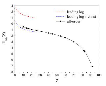
Figure 3: (Color online) Self-energy correction to the nuclear magnetic shielding.

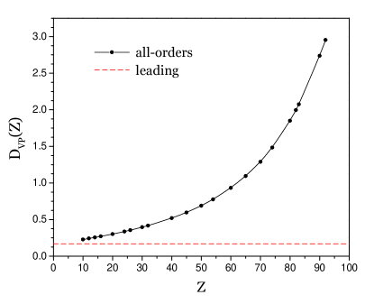
Figure 4: (Color online) Vacuum-polarization correction to the nuclear magnetic shielding.

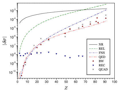
Figure 5: (Color online) Individual contributions to the nuclear shielding. “NR” is the nonrelativistic contribution, “REL” is the relativistic point-nucleus contribution, “FNS” is the finite nuclear size correction, “QED” is the QED correction, “BW” is the Bohr-Weisskopf correction, “REC” is the recoil correction, and “QUAD” is the electric quadrupole correction. Note that the QED correction changes its sign between $Z=4$ and 5.

The vacuum-polarization correction to the nuclear magnetic shielding is parameterized as

$$\Delta\sigma_{\rm VP}=\alpha^{2}\,({Z\alpha})^{3}\,D_{\rm VP}({Z\alpha})\,.$$ (125)

Our numerical results for the vacuum-polarization correction are presented in Table 2. The calculation was performed for the extended nucleus and the Uehling potential was included to all orders. Note that our present treatment is not complete, as the Wichmann-Kroll part of the correction is still missing. We estimate the uncertainty due to omitted terms to be within 30% of the calculated contribution.

The ${Z\alpha}$ expansion of the function $D_{\rm VP}$ reads

$$D_{\rm VP}({Z\alpha})=\frac{8}{9\pi n^{3}}\,\frac{3}{5}\,\delta_{l,0}+O({Z\alpha})\,,$$ (126)

where the Kronecker symbol $\delta_{l,0}$ indicates that the correction vanishes for the reference states with $l>0$. Comparison of the all-order numerical results with the leading term of the ${Z\alpha}$ expansion is given in Fig. 4. It is remarkable that the all-order results grow fast when $Z$ is increased and eventually become more than an order of magnitude larger than the leading-order result. In the high-$Z$ region, the self-energy and vacuum-polarization corrections are (as usual) of the opposite sign, the self energy being about twice larger than the vacuum polarization. In the low-$Z$ region, however, the self-energy correction changes its sign and the total QED contribution becomes positive for very light ions.

The summary of our calculations of the nuclear magnetic shielding constant $\sigma$ for several hydrogen-like ions is given in Table Acknowledgement. The first line of the table presents results for the leading-order nuclear shielding, including the finite nuclear size effect. The leading-order contribution was calculated using the Fermi model for the nuclear charge distribution and the point-dipole approximation for the interaction with the nuclear magnetic moment. The nuclear charge radii were taken from Ref. angeli:04 . The results are in good agreement with those reported in Ref. moskovkin:04 . The QED correction presented in the second line of Table Acknowledgement is the sum of the all-order results for the self energy and the vacuum polarization. Its error comes from the numerical uncertainty of the self-energy part and the estimate of uncalculated vacuum-polarization diagrams. Since there were no all-order calculations performed for oxygen, we used an extrapolation of our all-order results (taking into account the derived values of the ${Z\alpha}$ expansion coefficients).

The Bohr-Weisskopf correction, presented in the third line of Table Acknowledgement, was calculated by reevaluating the leading-order contribution with the point-dipole hfs interaction modified by the extended-distribution function $F(r)$ given by Eqs. (117) and (118). Because the effective single-particle model of the nuclear magnetic moment is (of course) a rather crude approximation, we estimate the uncertainty of the Bohr-Weisskopf correction to be 30%, which is consistent with previous estimates of the uncertainty of this effect shabaev:97:pra . This uncertainty includes also the error due to the nuclear polarization effect, which is not considered in the present work.

The quadrupole and the recoil corrections, given in the fourth and fifth lines of Table Acknowledgement, respectively, were evaluated according to Eqs. (121) and (119). The error of the quadrupole correction comes from the nuclear quadrupole moments. The magnetic dipole and electric quadrupole moments of nuclei were taken from Refs. raghavan:89 ; stone:05 .

The $Z$ dependence of individual contributions to the magnetic shielding constant $\sigma$ is shown in Fig. 5. The leading-order contribution is separated into three parts, the point-nucleus nonrelativistic part (solid line, black), the point-nucleus relativistic part (dashed line, green), and the finite nuclear size correction (dashed-dotted line, blue). We observe that the finite nuclear size correction, as well as the other effects calculated in this work, become increasingly important in the region of large nuclear charges. The only exception is the nuclear recoil correction. It practically does not depend on the nuclear charge number $Z$, since the linear $Z$ scaling in Eq. (119) is compensated by the increase of the nuclear mass $M$ with $Z$. As a consequence, the recoil effect is completely negligible for high- and medium-$Z$ ions, but turns into one of the dominant corrections for $Z<10$.

For most ions, the uncertainty of the theoretical prediction is roughly 30% of the Bohr-Weisskopf effect; it can be immediately estimated from Fig. 5. For very light ions, however, there is an additional uncertainty due to the unknown relativistic recoil effect. Its contribution can be estimated by multiplying the nonrelativistic recoil correction plotted on Fig. 5 by the factor of $({Z\alpha})^{2}$. We observe that for very light ions, the relativistic recoil is the dominant source of error in theoretical predictions.

VII Conclusion

In this work we have performed an ab initio calculation of the nuclear magnetic shielding in hydrogen-like ions with inclusion of relativistic, nuclear, and QED effects. The uncertainty of our theoretical predictions for the nuclear magnetic shielding constant defines [according to Eq. (8)] the precision to which the nuclear magnetic dipole moments can be determined from experiments on the $g$-factors of hydrogen-like ions. It can be concluded from Table Acknowledgement and Fig. 5 that the present theory permits determination of nuclear magnetic moments with fractional accuracy ranging from $10^{-9}$ in the case of ¹⁷O⁷⁺ to $10^{-5}$ for ²⁰⁹Bi⁸²⁺.

For most hydrogen-like ions, the dominant source of error in the theoretical predictions is the Bohr-Weisskopf effect. Since this effect cannot be accurately calculated at present, we conclude that the theory of the nuclear magnetic shielding has reached the point where the uncertainty due to nuclear-structure effects impedes further progress. For very light ions, however, the dominant theoretical error comes from the unknown relativistic recoil effect, whose calculation might be a subject of future work.

References

- (1) H. Häffner, T. Beier, N. Hermanspahn, H.-J. Kluge, W. Quint, S. Stahl, J. Verdú, and G. Werth, Phys. Rev. Lett. 85, 5308 (2000).
- (2) J. Verdú, S. Djekić, S. Stahl, T. Valenzuela, M. Vogel, G. Werth, T. Beier, H.-J. Kluge, and W. Quint, Phys. Rev. Lett. 92, 093002 (2004).
- (3) S. Sturm, A. Wagner, B. Schabinger, J. Zatorski, Z. Harman, W. Quint, G. Werth, C. H. Keitel, and K. Blaum, Phys. Rev. Lett. 107, 023002 (2011).
- (4) S. Sturm, A. Wagner, B. Schabinger, and K. Blaum, Phys. Rev. Lett. 107, 143003 (2011).
- (5) P. J. Mohr, B. N. Taylor, and D. B. Newell, Rev. Mod. Phys. 80, 633 (2008).
- (6) S. A. Blundell, K. T. Cheng, and J. Sapirstein, Phys. Rev. A 55, 1857 (1997).
- (7) H. Persson, S. Salomonson, P. Sunnergren, and I. Lindgren, Phys. Rev. A 56, R2499 (1997).
- (8) V. A. Yerokhin, P. Indelicato, and V. M. Shabaev, Phys. Rev. Lett. 89, 143001 (2002).
- (9) S. G. Karshenboim and A. I. Milstein, Physics Letters B 549, 321 (2002).
- (10) V. M. Shabaev and V. A. Yerokhin, Phys. Rev. Lett. 88, 091801 (2002).
- (11) K. Pachucki, U. D. Jentschura, and V. A. Yerokhin, Phys. Rev. Lett. 93, 150401 (2004), [(E) ibid., 94, 229902 (2005)].
- (12) K. Pachucki, A. Czarnecki, U. D. Jentschura, and V. A. Yerokhin, Phys. Rev. A 72, 022108 (2005).
- (13) T. Beier, H. Häffner, N. Hermanspahn, S. G. Karshenboim, H.-J. Kluge, W. Quint, S. Stahl, J. Verdú, and G. Werth, Phys. Rev. Lett. 88, 011603 (2002).
- (14) N. F. Ramsey, Phys. Rev. 78, 699 (1950).
- (15) B. Lahaye and J. Margerie, Opt. Commun. 1, 259 (1970).
- (16) M. G. H. Gustavsson and A.-M. Mårtensson-Pendrill, Phys. Rev. A 58, 3611 (1998).
- (17) D. L. Moskovkin, N. S. Oreshkina, V. M. Shabaev, T. Beier, G. Plunien, W. Quint, and G. Soff, Phys. Rev. A 70, 032105 (2004).
- (18) A. Rudziński, M. Puchalski, and K. Pachucki, J. Chem. Phys. 130, 244102 (2009).
- (19) V. A. Yerokhin, K. Pachucki, Z. Harman, and C. H. Keitel, Phys. Rev. Lett. 107, 043004 (2011).
- (20) G. Breit, Nature (London) 122, 649 (1928).
- (21) H. A. Bethe and E. E. Salpeter, Quantum Mechanics of One- and Two-Electron Atoms (Springer, Berlin, 1957).
- (22) E. A. Moore, Mol. Phys. 97, 375 (1999).
- (23) N. C. Pyper, Mol. Phys. 97, 381 (1999).
- (24) N. C. Pyper and Z. C. Zhang, Mol. Phys. 97, 391 (1999).
- (25) V. G. Ivanov, S. G. Karshenboim, and R. N. Lee, Phys. Rev. A 79, 012512 (2009).
- (26) V. M. Shabaev, Phys. Rep. 356, 119 (2002).
- (27) N. J. Snyderman, Ann. Phys. (NY) 211, 43 (1991).
- (28) V. A. Yerokhin and V. M. Shabaev, Phys. Rev. A 60, 800 (1999).
- (29) V. A. Yerokhin, P. Indelicato, and V. M. Shabaev, Eur. Phys. J. D 25, 203 (2003).
- (30) V. A. Yerokhin, K. Pachucki, and V. M. Shabaev, Phys. Rev. A 72, 042502 (2005).
- (31) V. A. Yerokhin, A. N. Artemyev, V. M. Shabaev, and G. Plunien, Phys. Rev. A 72, 052510 (2005).
- (32) V. A. Yerokhin and U. D. Jentschura, Phys. Rev. Lett. 100, 163001 (2008).
- (33) V. A. Yerokhin and U. D. Jentschura, Phys. Rev. A 81, 012502 (2010).
- (34) V. A. Yerokhin, P. Indelicato, and V. M. Shabaev, Phys. Rev. A 69, 052503 (2004).
- (35) V. M. Shabaev, K. Pachucki, I. I. Tupitsyn, and V. A. Yerokhin, Phys. Rev. Lett. 94, 213002 (2005).
- (36) V. M. Shabaev, I. I. Tupitsyn, K. Pachucki, G. Plunien, and V. A. Yerokhin, Phys. Rev. A 72, 062105 (2005).
- (37) L. Landau and E. M.Lifshitz, Quantum Mechanics: Non-Relativistic Theory. Vol. 3 (Pergamon Press, Oxford, England, 1977).
- (38) M. E. Rose, Relativistic Electron Theory (John Wiley & Sons, New York, 1961).
- (39) V. A. Yerokhin, A. N. Artemyev, T. Beier, G. Plunien, V. M. Shabaev, and G. Soff, Phys. Rev. A 60, 3522 (1999).
- (40) C. Itzykson and J. Bernard Zuber, Quantum Field Theory (McGraw-Hill, New York, 1980).
- (41) U. D. Jentschura, A. Czarnecki, and K. Pachucki, Phys. Rev. A 72, 062102 (2005).
- (42) A. Bohr and V. F. Weisskopf, Phys. Rev. 77, 94 (1950).
- (43) A. Bohr, Phys. Rev. 81, 331 (1951).
- (44) V. M. Shabaev, J. Phys. B 27, 5825 (1994).
- (45) V. M. Shabaev, M. Tomaselli, T. Kühl, A. N. Artemyev, and V. A. Yerokhin, Phys. Rev. A 56, 252 (1997).
- (46) O. M. Zherebtsov and V. M. Shabaev, Can. J. Phys. 78, 701 (2000).
- (47) L. Elton and A. Swift, Nucl. Phys. A94, 52 (1967).
- (48) E. Rost, Phys. Lett. 26B, 184 (1968).
- (49) I. Angeli, At. Data Nucl. Data Tables 87, 185 (2004).
- (50) P. Raghavan, At. Data Nucl. Data Tables 42, 189 (1989).
- (51) N. J. Stone, At. Data Nucl. Data Tables 90, 75 (2005).