Singular ways to search for the Higgs boson

Abstract

The discovery or exclusion of the fundamental standard scalar is a hot topic, given the data of LEP, the Tevatron and the LHC, as well as the advanced status of the pertinent theoretical calculations. With the current statistics at the hadron colliders, the workhorse decay channel, at all relevant $H$ masses, is $H\to WW,$ followed by $W\to\ell\nu$, $\ell=e$ or $\mu$. Using phase-space singularity techniques, we construct and study a plethora of “singularity variables” meant to facilitate the difficult tasks of separating signal and backgrounds and of measuring the mass of a putative signal. The simplest singularity variables are not invariant under boosts along the $pp$ or $p\bar{p}$ axes and the simulation of their distributions requires a good understanding of parton distribution functions, perhaps not a serious shortcoming during the boson hunting season. The derivation of longitudinally boost-invariant variables, which are functions of the four charged-lepton observables that share this invariance, is quite elaborate. But their use is simple and they are, in a kinematical sense, optimal.

It is nice to know that the computer
understands the problem. But I
would like to understand it too.
Eugene Wigner

I Introduction

Recent data from the LHC LHC on a putative standard Higgs boson exclude, at a 95% confidence level (CL), the mass domain 127 GeV $\!<M_{H}\!<$ 600 GeV (CMS) and, with some narrow gaps, 131 GeV $<\!M_{H}\!<$ 453 GeV (ATLAS). These results are obtained with full use of the standard theory, including radiative corrections which sometimes constitute the dominant effect. The amplitude for Higgs boson production, for example, is largely dominated by gluon fusion via a $t$-quark loop and so is the amplitude for $H\to\gamma\gamma$ decay.

In the “quantum-level” setting we recounted, it would be inconsistent not to analize the LHC data in conjunction with the constraints on $M_{H}$ which follow from the profusion of high precision measurements that test the standard theory beyond tree level. These constraints (and the direct searches CDFD0 at the Tevatron) result in $M_{H}\!<\!161\,(156)$ GeV at a CL of 95% LEPEW , while the direct LEP limit is $M_{H}\!>\!115$ GeV.

In mass intervals akin to the one implied by the quoted constraints CMS finds a 1.9$\sigma$ excess of events –that could be an indication of a Higgs signal– at $M_{H}=124$ GeV and ATLAS a 2.5$\sigma$ one at $M_{H}=126$ GeV LHC . In the current broad mass range(s) of the searches, the corresponding “local” significances are somewhat larger LHC , but have no rigorous statistical interpretation.

For a standard Higgs boson of mass $M_{H}>140$ GeV the branching ratio for the decay $H\to WW$ is the dominant one. Below this mass and above the LEP limit, the winner is $H\to b\bar{b}$, a process beset by terrifying backgrounds at a hadron collider. The branching ratio $W\to q\bar{q}$ is one order of magnitude larger than the one for $W\to\ell\nu$, $\ell=e,\mu$. But a light-lepton signal is much “cleaner” than that of a quark-generated jet. This makes the chain $H\to W^{+}W^{-}$, $W^{\pm}\to\ell^{\pm}\nu$ the all-mass workhorse at a hadron collider. In brief, we refer to this process as $H\to WW$, including the “off-shell” $M_{H}<2\,M_{W}$ case, often dubbed $H\to WW^{*}$.

The obvious problem with the $H\to WW$ channel is that $M_{H}$ cannot be reconstructed event by event, as a lot of information escapes detection with the unobserved neutrinos and, at a hadron collider, also with the unobserved hadrons that exit “longitudinally” close to the beam pipe(s). This makes taming the workhorse almost an art, not only a science. The formal and theoretically optimal singularity variable procedure to deal with this kind of incomplete information is summarized in Kim ; AA and exploited for the hadron-collider production of a single $W$ in AA . We shall see that, for the $H\to WW$ process, the situation is much more challenging, mainly because two missing neutrinos are many more than one.

The other crucial obstacles in the process we study are the large backgrounds with kinematics akin to those of the signal. The main and irreducible one is the direct non-resonant production of $W$ pairs by $q\bar{q}$ annihilation. The next most relevant one is $t\bar{t}$ production, which also results in $W$ pairs. For simplicity we shall illustrate our theoretical results only for the chain $W\to e\nu$, $W\to\mu\nu$, for which the “Drell-Yan” background is not a problem.

The analysis tools used to deal with the $H\to WW$ channel range from a simple “cut and count” approach to “matrix-element” techniques and avant-garde neural networks or “boosted decision trees” LHC . There is no question that in the long range the methods that input and utilize the largest amount of information are likely to be the most powerful ones. Whether this is also the case at an exploratory “Higgs-hunting” stage is more doubtful. Here we shall explore a “copy and paste” avenue of intermediate sophistication: the derivation of singularity variables –functions of the observable momenta and of $M_{H}$– whose measured histograms are to be compared (in one or more dimensions) with pre-prepared templates.

For the production of a Higgs boson at a hadron collider, followed by the decays $H\to W^{+}W^{-}$, $W^{\pm}\to\ell^{\pm}\nu$, we shall limit our discussion to the distributions of various functions of the charged lepton three-momenta $\vec{k}$ and $\vec{l}$. The treatment of the 2D transverse momentum of the final state hadrons, $\vec{p}_{T}$, deserves a separate paragraph, the next. The use of other observables, such as the number of jets, is beyond our scope.

Two practical problems are that $\vec{k}$ and $\vec{l}$ are measured to much higher precision than $\vec{p}_{T}$ and that the formulae for the $H\to WW$ singularity variables are much more complex for $\vec{p}_{T}\neq 0$ than for $\vec{p}_{T}=0$. We deal with both problems by setting $\vec{p}_{T}=0$ in our theoretical expressions. This is less cavalier than it seems. The transverse momentum of a Higgs boson in a given event is $\simeq\!-\mspace{1.0mu}\vec{p}_{T}$. For a given ansatz $M_{H}$ value, its observed lepton momenta can be Lorentz boosted closer to the $\vec{p}_{T}=0$ frame. The precise boost would require knowledge of the boson’s longitudinal momentum, $p_{3}$. But, typically, $p_{3}^{2}\ll 2\mspace{1.0mu}M_{H}^{2}$, it is a fair approximation to neglect $p_{3}$. More importantly, the singularity variables for $\vec{p}_{T}=0$ are very useful even in the analysis of events with $\vec{p}_{T}\neq 0$, even if one does not boost the events back closer to the $\vec{p}_{T}=0$ frame, and even if one is also dealing with the quoted backgrounds, whose $W$ pairs do not have a fixed invariant mass.

Let the lepton momenta be $\vec{k}\equiv\{\vec{k}_{T},k_{3}\}$ and $\vec{l}\equiv\{\vec{l}_{T},l_{3}\}$. Because of the rotational symmetry along the beams’ axis, the six-dimensional observable space $\{\vec{k},\vec{l}\}$ is in practice just five-dimensional. One possible choice of variables is the set $(k+l)^{2}$, the invariant mass of the lepton pair; $k_{T}$, $l_{T}$, the moduli of the transverse momenta; and $\vec{k}_{T}\cdot\vec{l}_{T}$, or the familiar $\Delta\varphi=\arccos[\vec{k}_{T}\cdot\vec{l}_{T}/(k_{T}\,l_{T})]$. All four of these “transverse” observables are invariant under longitudinal boosts along the beams’ axis. The remaining variable, for instance $k_{3}+l_{3}$, is not.

We shall derive two types of singularity variables: those which do –or do not– depend only on transverse observables. Transverse variables are preferable, in that they are insensitive to the significant uncertainties associated with the (longitudinal) parton distribution functions (pdfs). In practice the uncertainties are to a modest extent reintroduced via the angular coverage limitations of an actual experiment, which are not invariant under longitudinal boosts. The histograms of singularity variables that are not longitudinally invariant do depend on the pdfs, but, particularly during a Higgs-hunting or initiatory epoch, this is not a serious limitation.

In the problem at hand, the quintessential function of transverse variables –in the sense of its ability to tell apart signal from backgrounds– is $\Delta\varphi$, the angle between the charged leptons in the transverse plane. In Fig. 1, for comparison with our coming results, we recall this fact by showing the (arbitrarily normalized) shapes of signal and background distributions for two examples, with $M_{H}=500$ and 120 GeV. As is well known, the V-A nature of the weak current and the specific spin zero nature of the $W$ pair in signal events, favours collinear vs. anticollinear leptons. The effect weakens as $M_{H}$ increases and the leptons are boosted away from each other.

The simulations of Fig. 1, as well as all others in this note, were made with use of the PYTHIA6 event generator SMS . They are for the $H\to WW$, $W\to e\nu$, $W\to\mu\nu$ channel, with leptons of transverse momentum greater than 15 GeV, and satisfying the pseudorapidity cuts $\eta(e)<2.5$, $\eta(\mu)<2.1$.

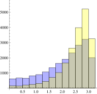
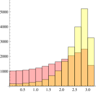
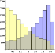
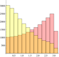
Figure 1: Distributions of $\Delta\varphi$. Top row: $M_{H}=500$ GeV. Bottom row: $M_{H}=120$ GeV. Left column: Comparison between the shape of the (yellow) signal distribution and that of the (blue) $WW$ background. Right column: Comparison of signal with the (orange) $t\bar{t}$ background.

Our goal is two-fold. First and foremost, to derive the complete set of phase-space singularity variables (functions analogous to $\Delta\varphi$) for the process at hand. Second, to illustrate with examples their potential phenomenological usage. At least at low $M_{H}$ values, $\Delta\varphi$ is more heavily dependent on dynamics than on kinematics. The singularity variables we shall derive are the other way around. Individually, several of them are nearly “as good” as $\Delta\varphi$ in disentangling a signal from the backgrounds. The ensemble of their distributions, particularly in conjunction with $\Delta\varphi$ itself, should be a powerful and relatively simple tool to search for a Higgs boson, which, in the sense of signal kinematics, is guaranteed to be optimal.

Since we investigate a plethora of singularity variables, this paper is long and detailed. The reader mainly interested in results may be well advised to start reading it from the end: §XI and §XII.

II Outline

The simple example of single-$W$ production is used in §III to clarify what singularity conditions and singularity variables are. After posing the formal problem in §IV we proceed in §V to solve it in the center of mass (CM) reference system of the Higgs boson. There are two reasons for this. First, it is a necessary intermediate step in the theoretical derivation, in §VI, of the general case with a boson which is not at rest. Second, the “approximation” of a heavy particle made at rest by gluon-gluon or $q\bar{q}$ fusion in a hadron collider is not so bad, since the quark and gluon pdfs are fast falling functions of their fractional momenta. Our results will reflect this fact.

We shall have to deal with the case $M_{H}<2\mspace{1.0mu}M_{W}$, in which at least one of the $W$s is off-shell; the relative probability for both of them having an invariant mass significantly different from $M_{W}$ is small. In §VII we explain the simple way in which we treat this case. Further details of our data analysis not already discussed in the introduction are given in §VIII.

We analize MC-generated data in §IX in the theoretical approximation of a Higgs boson made at rest. To some extent, this section is a “warm-up” for the general results wherein we lift this approximation, discussed in §X, to which the reader interested in the most powerful results may prefer to jump.

A summary of results is given in §XI. Our data analysis is not as thorough as the theoretical one, it is only meant to illustrate our points. But it suffices to reach our conclusions, which, naturally, are drawn in the last section. A very formal but important step in our theoretical analysis is relegated to the Appendix.

III Simple singularity variables

Our main result is the theoretical derivation of the phase space singularity variables and singularity conditions for the process $H\to W^{+}W^{-}$, $W^{\pm}\to\ell^{\pm}\nu$. To understand these concepts it is easiest to recall a simpler problem: the analogous one for single-$W$ production at a hadron collider, followed by the same leptonic decay. In this case, the singularity condition AA is $\Sigma_{T}=0$, with:

$$\Sigma_{T}(M,\vec{l}_{{}_{T}},\vec{p}_{{}_{T}})\equiv$$

$$M^{4}-4\,M^{2}\,(\vec{l}_{{}_{T}}\cdot\vec{p}_{{}_{T}}+l_{{}_{T}}^{2})+4\,\left[(\vec{l}_{{}_{T}}\cdot\vec{p}_{{}_{{}_{T}}})^{2}-l_{{}_{T}}^{2}\,p_{{}_{T}}^{2}\right]$$ (1)

Of the four $M$-roots of $\Sigma_{T}=0$, one is not unphysical:

$${M_{T}}(\vec{l}_{{}_{T}},\vec{p}_{{}_{T}})\!=\!+\sqrt{2\,\left[|l_{{}_{T}}|\,|p+l|_{{}_{T}}+\vec{l}_{{}_{T}}\cdot(\vec{l}_{{}_{T}}+\vec{p}_{{}_{T}})\right]},$$ (2)

which reduces to ${M_{T}}\!=\!2\,|l_{{}_{T}}|$ for $\vec{p}_{{}_{T}}\!=\!0$. The function in Eq. (2) is the habitual $M_{{}_{T}}^{2}$ originally derived in mT2A ; mT2B .

The result of Eq. (1) is obtained by projecting the full phase space (which includes the neutrino momentum) onto the observable phase space. The function $\Sigma_{T}$ is a singularity variable which –for a general non-singular event– is a measure of its distance to the nearest singularity at the singular $\Sigma_{T}=0$ border of the projected space. In Eq. (1) the mass of the $W$ appears in two ways: the physical $M_{H}$ is imprinted in the data and also appears as an implicit “trial” mass $M\to\cal M$ in the equation. In the $M_{T}$ singularity variable of Eq. (2) $M_{H}$ is only reflected in the observables. In applying the phase-space singularity approach to our two-$W$ problem, we shall encounter both types of singularity variables.

In the single-$W$ case one can refine the result in the sense of finding the optimal singularity variable, that which would result in the most precise measurement of $M_{W}$ AA . In the two-$W$ case this is not worthwhile, as there are decay channels, such as $H\to\gamma\gamma$, $H\to ZZ$; $Z\to\ell^{+}\ell^{-}$, for which the mass is reconstructible.

IV The formal problem

Back to the $H\to W^{+}W^{-}$, $W^{\pm}\to\ell^{\pm}\nu$ process, let $y$ and $x$, respectively, be the four-momenta of the neutrinos accompanying the charged leptons of four-momentum $k$ and $l$. The full information relevant to the reconstruction of the boson’s mass for a signal event is embedded in the kinematical equations:

$$E_{1}\Rrightarrow x^{2}=0$$

$$E_{2}\Rrightarrow y^{2}=0$$

$$E_{3}\Rrightarrow 2\,l\cdot x=M_{W}^{2}$$

$$E_{4}\Rrightarrow 2\,k\cdot y=M_{W}^{2}$$

$$E_{5}\Rrightarrow 2\,(l+x)\cdot(k+y)=M_{H}^{2}-2\,M_{W}^{2}$$

$$E_{6}\Rrightarrow k_{1}+y_{1}+l_{1}+x_{1}+p_{1}=0$$

$$E_{7}\Rrightarrow k_{2}+y_{2}+l_{2}+x_{2}+p_{2}=0$$ (3)

where we have made the approximation $l^{2}=k^{2}=0$ for the charged leptons and –fleetingly in error for the $WW^{*}$ case– set the masses of the two $W$s to their central values. There are 9 unknowns (2 neutrino four-momenta and $M_{H}$) and only 7 equations. In spite of this, is there a systematic way to extract the kinematically most stringent information on $M_{H}$? This is the problem to face.

Consider the 14D space of the components $\vec{l},\vec{k}$ of the three-momenta of the two (approximately massless) charged leptons and the four-momenta $x,y$ of the two neutrinos. For a fixed $M_{H}$, the seven Equations (3) define a $14-7=7$D manifold, the phase space. This surface is to be projected onto the 6D hyper-plane of observable three-momenta. The points in the full phase space that project onto the boundary of the 6D space of observables are singular: at such points one or more of the invisible directions are contained in the tangent plane to the full phase space Kim ; AA , and a tangent to a surface is singular in that it “touches it” at more than one single point.

The equation, $\Sigma(\vec{l},\vec{k},M_{W}^{2};M_{H}^{2})=0$, describing the boundary of the projected phase space is a singularity condition. A general event (i.e. specific values of $\vec{l}$ and $\vec{k}$) is non-singular and its corresponding value of $\Sigma$ is, once again, a measure of distance to the $\Sigma=0$ singularity. The shape of the distribution of the values of the singularity variable $\Sigma$ is sensitive to the unknown mass $M_{H}$ in a manner that allows one to extract its true value, be it physical or Monte Carlo (MC) generated.

The formal modus operandi to obtain singularity variables is summarized in Kim and discussed in detail in AA . We recalled that at a singularity one or more of the invisible directions are contained in the tangent plane to the full phase space. The general condition for this to happen is that, in the space $\{z\}=\{x,y\}$ of invisible directions, the row vectors of the Jacobian matrix $J_{ij}\equiv\partial E_{i}/\partial z_{j}$ (with the row index $i$ running along the number of equations and the column index $j$ over the number of invisible coordinates) be linearly dependent. In other words, at a singularity, the rank of $J_{ij}$ must be smaller than its rank at nonsingular points.

There are 7 equations and 8 invisible directions in Eqs. (3). The vanishing of the Jacobian $J_{ij}$ (a $7\times 8$ matrix) entails 8 conditions: the nullification of all $7\times 7$ minors. Two of these minors coincide, up to their sign, with two others. Moreover the sums of two pairs of minors are of the forms $D\,{\cal S}_{0}$, $D\,{\cal S}_{3}$, with

$$\begin{split}&D\equiv\det(l,x,k,y)\\ &{\cal S}_{0}\equiv k_{0}+l_{0}+x_{0}+y_{0},\\ &{\cal S}_{3}\equiv k_{3}+l_{3}+x_{3}+y_{3}.\end{split}$$ (4)

Given that ${\cal S}_{0}>0$, one condition is:

$$\det(l,x,k,y)=0,$$ (5)

that is, the coplanarity of the four lepton four-momenta, equivalent to

$$y=\alpha\,l+\beta\,x+(\gamma-1)\,k.$$ (6)

Introducing this into the 8 original minors, it is easy to see that they all vanish provided that

$$\gamma={{(\alpha-\beta)\,(l_{3}\,x_{0}-l_{0}\,x_{3})}\over\alpha\,(k_{3}\,l_{0}-k_{0}\,l_{3})+\beta\,(k_{3}\,x_{0}-k_{0}\,x_{3})}$$ (7)

The transposed Jacobian matrix, with use of E6 and E7 of Eqs. (3), is

$$J({\cal S}_{0},{\cal S}_{3})=\left(\begin{array}[]{ccccccc}x_{0}&0&l_{0}&0&{\cal S}_{0}&0&0\\ -x_{1}&0&-l_{1}&0&0&1&0\\ -x_{2}&0&-l_{2}&0&0&0&1\\ -x_{3}&0&-l_{3}&0&-{\cal S}_{3}&0&0\\ 0&y_{0}&0&k_{0}&{\cal S}_{0}&0&0\\ 0&-y_{1}&0&-k_{1}&0&1&0\\ 0&-y_{2}&0&-k_{2}&0&0&1\\ 0&-y_{3}&0&-k_{3}&-{\cal S}_{3}&0&0\end{array}\right),$$ (8)

where the functional dependence of $J$ on ${\cal S}_{0,3}$ has been made explicit for later convenience.

It turns out to be very useful to study the behaviour of the $7\times 7$ minors of $J$ under longitudinal Lorentz transformations, the boosts along the axis “3” of the proton beams. To proceed recall that, for the reasons stated in the Introduction, we are setting the hadron momenta $p_{1}=p_{2}=0$. Next, parametrize an event in the usual Cabibbo-Maximovich manner CM , illustrated in our notation in Fig. 2. That is, consider the lepton momenta as if both $W$ bosons were at rest, boost them by the antiparallel motion of the $W$s in the $H$ rest system and finally boost the Higgs boson longitudinally left or right along the beams’ axis:

$$\begin{split}&l=L(y_{H},\vec{n}_{p})\,L(y,\vec{n})\,(M_{W}/2)\{1,\vec{n}_{l}\},\\ &x=L(y_{H},\vec{n}_{p})\,L(y,\vec{n})\,(M_{W}/2)\{1,-\vec{n}_{l}\},\\ &k=L(y_{H},\vec{n}_{p})\,L(y,-\vec{n})\,(M_{W}/2)\{1,\vec{n}_{k}\},\\ &y=L(y_{H},\vec{n}_{p})\,L(y,-\vec{n})\,(M_{W}/2)\{1,-\vec{n}_{k}\},\end{split}$$ (9)

where $\vec{n}_{k},\vec{n}_{l},\vec{n}$ and $\vec{n}_{p}$ are unit vectors, $L(y,\vec{n})$ is a Lorentz boost along $\vec{n}$ with velocity $\beta=\tanh(y)$, $y={\rm arccosh}(\gamma)$, $\gamma=M_{H}/(2\,M_{W})$, and analogously for the longitudinal boost along $n_{p}$, of rapidity $y_{H}$.

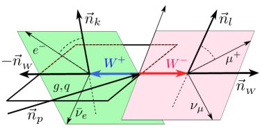
Figure 2: Top: The $H\to WW$, $W\to\ell\nu$ process in a Cabibbo-Maximovich parametrization CM . The vectors $\vec{n}_{l}$ and $\vec{n}_{k}$ are the directions of the charged leptons (a $\mu^{+}$ and an $e^{-}$ in this illustration) in the respective rest systems of their parent $W$s. The overall $WW$ system, shown here at rest, is to be boosted along the direction $\vec{n}_{p}$ of the gluon or $q\bar{q}$ pair that fuse to produce the $W$ pair, resonantly (for the $H$ signal) or not (for the irreducible background).

Label $m_{j}$, $j=1$ to 8, the $7\times 7$ minors of $J$ in Eq. (8), lacking the row $9-j$ of $J$. Under a longitudinal boost $L(y_{H},\vec{n}_{3})$, they transform as $m_{j}\mapsto\bar{m}_{j}$, with:

$$\begin{split}&\bar{m}_{1}=\gamma_{H}\,[m_{1}+\beta_{H}\,m_{8}+\beta_{H}\,{\cal S}_{3}\,D],\\ &\bar{m}_{i}=m_{i},\;\;\;i=2,\,3,\,6,\,7,\\ &\bar{m}_{4}=\gamma_{H}\,[m_{4}+\beta_{H}\,m_{5}-\beta_{H}\,{\cal S}_{0}\,D],\\ &\bar{m}_{5}=\gamma_{H}\,[m_{5}+\beta_{H}\,m_{4}+\beta_{H}\,{\cal S}_{3}\,D],\\ &\bar{m}_{8}=\gamma_{H}\,[m_{8}+\beta_{H}\,m_{1}-\beta_{H}\,{\cal S}_{0}\,D],\end{split}$$ (10)

where we used the definitions in Eqs. (4).

The conditions $m_{j}=0,\;\forall\,j$ imply that $D=0$, and consequently that $\bar{m}_{j}=0,\;\forall\,j$. Thus, we reach a crucial point: the general singular configurations can be obtained by boosts of the ones in the boson’s rest system. This is one of the reasons why we pause to study this latter simpler case.

V Lessons from a gluon collider

A standard Higgs can be made in various ways, with top-mediated gluon fusion being the dominant mechanism up to very high $M_{H}$ values. The gluonic pdfs, as well as those of the other partons, are fast-falling functions of their fractional momentum. This implies that Higgs bosons are made with a narrow distribution of rapidities, centered at $y_{H}=0$. The same is true for the backgrounds to the $H\to WW$ channel, e.g. non-resonant pairs of relatively heavy objects, such as $W$-bosons, are also made with a moderate collective motion. Thus, the approximation of a monochromatic “gluon collider” (or $q\bar{q}$ collider) is a good starting point for our analysis.

V.1 Derivation of the singularity conditions

In the $WW$ center of mass (CM) system an extra working condition is to be added to Eqs. (3):

$$C_{\rm CM}\Rrightarrow{\cal S}_{3}\equiv l_{3}+x_{3}+k_{3}+y_{3}=0.$$ (11)

and the Jacobian is now $J({\cal S}_{0},0)$, with $J$ as in Eq. (8). Since ${\cal S}_{0}>0$ and the fifth column of $J({\cal S}_{0},0)$ is proportional to ${\cal S}_{0}$, it suffices to consider the vanishing of the eight $7\times 7$ minors of $J(1,0)$, of which only four, e.g. $m_{i}$, $i=1,...4$, are independent modulo $D$.

In the CM system, let $E=M_{H}/2$ denote the $W$’s energy and $P$ the corresponding momentum modulus. The four-momenta of the individual $W$s in the notation of Eq. (9) are:

$$p_{{}_{Wl}}=\{E,+P\,{\vec{n}}\}$$

$$p_{{}_{Wk}}=\{E,-P\,{\vec{n}}\}$$ (12)

and it is convenient to put the neutrino’s momenta in the form $x=p_{{}_{Wl}}-l$, $y=p_{{}_{Wk}}-k$.

The conditions $x^{2}=y^{2}=0$ now read

$$\begin{split}&2\mspace{1.0mu}E\mspace{1.0mu}l_{0}=M_{W}^{2}+2P\,\vec{l}\cdot\vec{n}\\ &2\mspace{1.0mu}E\mspace{1.0mu}k_{0}=M_{W}^{2}-2P\,\vec{k}\cdot\vec{n}.\end{split}$$ (13)

Stepping back to Eq. (8) and introducing the explicit lepton four-momenta in the minors of $J(1,0)$ and in $\det(l,x,k,y)$, the vanishing of the results requires, in particular, that $\det(\vec{l},\vec{k},\vec{n})=0$, that is, the 3D coplanarity of $\vec{l},\vec{k}$ and $\vec{n}$ and, consequently, of all four lepton three-momenta. We may write

$$\vec{n}=(a/l_{0})\vec{l}+(b/k_{0})\vec{k}.$$ (14)

Gathering results and imposing $\vec{n}\cdot\vec{n}=1$, one may express $a,b,x$ and $y$ as functions of $l$ and $k$. Two families of CM critical configurations are obtained. They differ by the sign of $\delta$ in

$$\delta^{2}=(4k_{0}^{2}-2M_{H}k_{0}+M_{W}^{2})(4l_{0}^{2}-2M_{H}l_{0}+M_{W}^{2})$$ (15)

and satisfy:

$$\vec{k}\cdot\vec{l}={-4E^{2}k_{0}l_{0}+2E(k_{0}+l_{0})M_{W}^{2}-M_{W}^{4}+M_{W}^{2}\delta\over 4\mspace{1.0mu}P^{2}},$$

$$a=\dfrac{l_{0}\big{[}-2Ek_{0}(\vec{k}\cdot\vec{l}+k_{0}l_{0})+(k_{0}^{2}+\vec{k}\cdot\vec{l})M_{W}^{2}\big{]}}{2\big{[}(\vec{k}\cdot\vec{l})^{2}-k_{0}^{2}l_{0}^{2}\big{]}\mspace{1.0mu}P},$$

$$b=\dfrac{k_{0}\big{[}2El_{0}(\vec{k}\cdot\vec{l}+k_{0}l_{0})-(l_{0}^{2}+\vec{k}\cdot\vec{l})M_{W}^{2}\big{]}}{2\big{[}(\vec{k}\cdot\vec{l})^{2}-k_{0}^{2}l_{0}^{2}\big{]}\mspace{1.0mu}P},$$ (16)

Substituting these expressions into $m_{i}$, $i=1,...4$ one finds that $m_{4}$ vanishes automatically. The others independent minors acquire the form

$$\begin{split}&m_{1}=(k_{2}l_{1}-k_{1}l_{2})\,{\cal N}/{\cal D},\\ &m_{2}=(k_{3}l_{1}-k_{1}l_{3})\,{\cal N}/{\cal D},\\ &m_{3}=(k_{3}l_{2}-k_{2}l_{3})\,{\cal N}/{\cal D},\end{split}$$ (17)

where $\cal N$ and $\cal D$ are lengthy functions of $k$ and $l$.

There are two alternative ways to satisfy $m_{i}=0$ $\forall i$. One of them is to let all three parenthesis in Eqs. (17) vanish simultaneously, tantamount to imposing $\vec{k}\propto\vec{l}$, a specific case of the condition to be obtained anon from the second alternative: ${\cal N}=0$. Eliminating the sign ambiguity of $\delta$ yields a first requirement for an event to be singular, $C=0$, with

$$\begin{split}&C=\kappa\,C_{1}^{2}\,C_{2}^{3}\,C_{3},\\ &\kappa\equiv-\mspace{1.0mu}2\mspace{1.0mu}M_{H}^{10}M_{W}^{4}\left(M_{H}^{2}-4M_{W}^{2}\right)^{3},\\ &C_{1}\equiv k_{0}-l_{0},\\ &C_{2}\equiv 2k_{0}l_{0}M_{H}-M_{W}^{2}(k_{0}+l_{0}),\\ &C_{3}\equiv 4M_{W}^{2}(k_{0}l_{3}+k_{3}l_{0})\big{[}2M_{H}(k_{0}k_{3}+l_{0}l_{3})+{}\\ &2(k_{0}-l_{0})(k_{0}l_{3}-k_{3}l_{0})-M_{H}^{2}(k_{3}+l_{3})\big{]}+{}\\ &M_{W}^{4}(k_{3}+l_{3})\big{[}M_{H}(k_{3}+l_{3})-2(k_{0}-l_{0})(k_{3}-l_{3})\big{]}+{}\\ &4M_{H}(2k_{0}-M_{H})(2l_{0}-M_{H})(k_{0}l_{3}+k_{3}l_{0})^{2}\end{split}$$ (18)

The non-trivial vanishing of $C_{3}$ implicitly presupposes ${\rm det}(\vec{l},\vec{k},\vec{n})=0$. Up to non-vanishing overall factors, a second requirement for an event to be singular is this coplanarity condition, squared such as to eliminate the sign of $\delta$: $C_{0}=0$, with

$$\begin{split}\\ &C_{0}=2\mspace{1.0mu}M_{W}^{2}(l\!\cdot\!k-2k_{0}l_{0})\big{[}2\mspace{1.0mu}l\cdot k-M_{H}(k_{0}+l_{0})\big{]}\\ &-M_{H}^{2}(l\!\cdot\!k-2k_{0}l_{0})^{2}+M_{W}^{4}\big{[}2\mspace{1.0mu}l\!\cdot\!k-(k_{0}+l_{0})^{2}\big{]},\end{split}$$ (19)

where $l\!\cdot\!k$ has its customary Minkowskian meaning.

V.2 Questions of nomenclature

For a singular event the values of $C$ in Eq. (18) and $C_{0}$ in Eq. (19) must both vanish. Given the form of $C$, there are three nontrivial ways for this to happen: $C_{i}\!=\!C_{0}\!=\!0$, $i=1$ to 3, which we call complete singularity conditions. Of these, only $C_{3}\!=\!C_{0}\!=\!0$ guarantees that all minors of the Jacobian vanish. The other two conditions, $C_{i}\!=\!C_{0}\!=\!0$, $i=1$ to 2, are mock singularity conditions, in a sense occasionally used in mathematics, that is, they do not satisfy all wanted conditions, but are useful for one’s purposes. As it turns out, even the four partial singularity conditions $C_{j}\!=\!0$, $j=0$ to 3, are of interest.

We choose $C_{0}$ as the example to make our next linguistic points. Consider a real or MC-generated event due to the production and decay of a Higgs boson. Its corresponding value of the $C_{0}$ function in Eq. (19) –a (partial) measure of distance to the $C_{0}\!=\!0$ singularity– depends on the Higgs boson mass in two distinct senses. The first is that $k_{0}$, $l_{0}$ and $l\!\cdot k\!$ are contingent on this “input” mass. The second is the explicit $M_{H}$ in the expression of $C_{0}$, which is a variable that one may –naturally– vary at will. To emphasize this point, we label this analyst’s mass calligraphically: $M_{H}\to{\cal M}$.

It is convenient to rescale and rewrite $C_{0}$ as:

$$C_{0}=-\,M_{E}^{4}\;\Sigma_{0}({\cal M})/4$$

$$\Sigma_{0}({\cal M})\equiv({\cal M}-M_{+})({\cal M}-M_{-})$$

$$M_{\pm}=\frac{2M_{W}}{M_{E}^{2}}\left[M_{W}({k_{0}}+{l_{0}})\pm M_{M}\sqrt{M_{W}^{2}-M_{E}^{2}}\right]$$

$$M^{2}_{M,E}\equiv 2\mspace{1.0mu}(k_{0}\mspace{1.0mu}l_{0}\mp\vec{k}\,\vec{l}\;),$$ (20)

where $M_{\pm}$ are the non-zero roots of $C_{0}=0$ and $M^{2}_{M,E}$ are the Minkowski and “Euclidean” masses of the (approximately massless) charged lepton pair. Notice that $\Sigma_{0}$ depends on the implicit variable $\cal M$, while its roots, $M_{\pm}$ do not. That is why we refer to $\Sigma_{0}$ and $M_{\pm}$ with different symbols, even though their distributions are in all cases diagnostics of the value of the real or simulated Higgs boson mass (we reserve the nomenclature “$M$” for all singularity variables of the later kind). Implicit masses become theoretically inevitable in cases for which, unlike for $\Sigma_{0}$, the ${\cal M}$ roots cannot be made explicit.

Functions of an implicit mass $\cal M$, such as $\Sigma_{0}$, are also singularity variables. They vanish at singular points of phase space, iff the correct choice ${\cal M}=M_{H}$ has been made, with $M_{H}$ the physical or Monte Carlo “truth”.

V.3 Partial and complete singularity conditions and variables

The singularity condition $C=0$ of Eq. (18) can be satisfied in various ways. Two of them ($M_{H}=0$ and $M_{H}=2\,M_{W}$) are of little practical relevance. Two others correspond to the naïve-looking observables

$$M_{1} = |k_{0}-l_{0}|$$ (21)

$$M_{2} = M_{W}^{2}\,{k_{0}+l_{0}\over 2\,k_{0}\,l_{0}}$$ (22)

The remaining possibility is $C_{3}=0$ in Eq. (18), a cubic polynomial in the Higgs boson mass. In analogy with Eq. (20) for $C_{0}$, we introduce its roots:

$$C_{3}=F\;\Sigma_{3}({\cal M})$$

$$\Sigma_{3}({\cal M})=({\cal M}-\tilde{M}_{1})({\cal M}-\tilde{M}_{2})({\cal M}-\tilde{M}_{3})$$

$$F\equiv 4\,(k_{3}\,l_{0}+k_{0}\,l_{3})^{2}$$ (23)

where the explicit forms of $\tilde{M}_{i}$ are lengthy.

It is not useless to rewrite Eqs.(20,22,23) in the form:

$$\tilde{\Sigma}_{0} \equiv {\rm Sign}(\Sigma_{0})\,|\Sigma_{0}|^{1/2}$$

$$\Sigma_{1} \equiv M_{1}$$

$$\Sigma_{2} \equiv {\cal M}-M_{2}$$

$$\tilde{\Sigma}_{3} \equiv {\rm Sign}(\Sigma_{3})\,|\Sigma_{3}|^{1/3}$$ (24)

This is because to construct true singularity variables that reflect a complete set of singularity conditions we must introduce a measure of the distance between a data point (given values of $\vec{k}$ and $\vec{l}\,$) and one of the three center-of-mass singular manifolds: the points $\{0,0\}$ of the planes $\{C_{i}=0\}\cap\{C_{0}=0\}$, $i=1$ to 3. With the help of Eqs. (20,24) we define the following quantities with unit mass dimension:

$$D_{1} = \left(\tilde{\Sigma}_{0}^{2}+\Sigma_{1}^{2}\right)^{1/2}$$

$$D_{2} = \left(\tilde{\Sigma}_{0}^{2}+\Sigma_{2}^{2}\right)^{1/2}$$

$$D_{3} = \left(\tilde{\Sigma}_{0}^{2}+\tilde{\Sigma}_{3}^{2}\right)^{1/2}$$ (25)

The functions $D_{i}({\cal M})$ are the full set of complete center-of-mass singularity variables for the case at hand.

V.4 From Algebra to Geometry

An advantage of the approximation in which Higgs bosons would be produced at rest is that the locus of the singular points in the observable $\{\vec{k},\vec{l}\}$ phase space can be visualized. Let $c_{\varphi}\equiv\cos\Delta\varphi=\vec{k}_{T}\cdot\vec{l}_{T}/(k_{T}\,l_{T})$. The singular phase space is shown in Fig. 3 in the variables $\{k_{0},l_{0},c_{\varphi}\}$, in an example wherein we have chosen $M_{H}=2.5$ in $M_{W}=1$ units. The closed surface in the three subfigures is the coplanarity condition $C_{0}=0$, see Eq. (19). The thick lines in the top and middle figure correspond to the singularity conditions $C_{0}=C_{1}=0$ and $C_{0}=C_{2}=0$, see Eqs (18). The last figure partly describes the singular phase space $C_{0}=C_{3}=0$ for the choice $k_{3}+l_{3}=0$; the complete space would be the direct product of this latter line in $\{k_{3},l_{3}\}$ space with the thick line in the figure.

The $C_{0}=C_{3}=0$ singularity condition, as one varies $k_{3}+l_{3}$, covers all of the $C_{0}=0$ coloured surface of Fig. 3. This reflects the fact that the other two conditions are mock, and of zero measure relative to $C_{0}=C_{3}=0$.

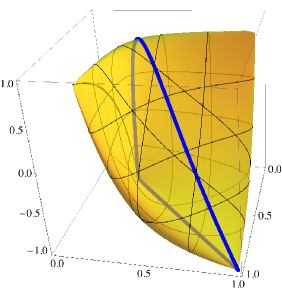
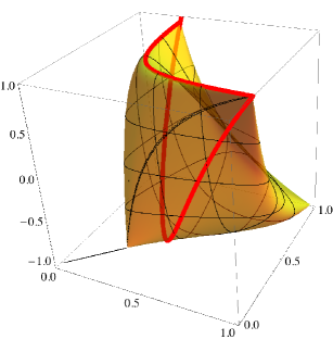
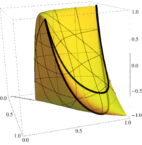
Figure 3: Visualizing the singular CM phase space. The closed surface in all figures is $C_{0}=0$, see Eq. (19). The thick lines in the top (middle) figure are the singularity conditions $C_{0}=C_{1}=0$ ($C_{0}=C_{2}=0$), see Eqs (18). The thickest black line in the bottom figure is the singular phase space $C_{0}=C_{3}=0$ for the particular choice $k_{3}+l_{3}=0$. The entire illustration is for $M_{W}=1,M_{H}=2.5$. The horizontal axes are $k_{T}$ and $l_{T}$, the vertical one is $c_{\varphi}\equiv\vec{k}_{T}\cdot\vec{l}_{T}/(k_{T}\,l_{T})$.

VI Back to a hadron Collider

The derivation of a singularity variable for the more realistic case of an $H$ boson of rapidity $y_{H}\neq 0$ is akin to that of the $y_{H}=0$ case, requiring only one extra step. Naturally, this is to start by applying the Lorentz boost $L(y_{H},\vec{n}_{p})$ to the $W$ momenta of Eq. (12), to obtain:

$$p_{{}_{Wl}}\!=\!\{c\mspace{1.0mu}E+s\mspace{1.0mu}P\mspace{1.0mu}n_{3},+P\mspace{1.0mu}n_{1},+P\mspace{1.0mu}n_{2},c\mspace{1.0mu}P\mspace{1.0mu}n_{3}+s\mspace{1.0mu}E\}$$

$$p_{{}_{Wk}}\!=\!\{c\mspace{1.0mu}E-s\mspace{1.0mu}P\mspace{1.0mu}n_{3},-P\mspace{1.0mu}n_{1},-P\mspace{1.0mu}n_{2},c\mspace{1.0mu}P\mspace{1.0mu}n_{3}-s\mspace{1.0mu}E\}$$ (26)

where $c\equiv\cosh(y_{H})$ and $s\equiv\sinh(y_{H})$. Following precisely the same steps as in §V.1, one concludes that the partial singularity conditions are $C^{\prime}_{i}=0$, $i\!=\!1$ to 4, with

$$C_{1}^{\prime} = 2\mspace{1.0mu}\xi\mspace{1.0mu}C_{1}(l_{0}^{\prime},l_{3}^{\prime},k_{0}^{\prime},k_{3}^{\prime})$$

$$= k_{0}+k_{3}-l_{0}-l_{3}+\left(k_{0}-k_{3}-l_{0}+l_{3}\right)\xi^{2}$$

$$C_{2}^{\prime} = 2\mspace{1.0mu}\xi^{2}\mspace{1.0mu}C_{2}(l_{0}^{\prime},l_{3}^{\prime},k_{0}^{\prime},k_{3}^{\prime})$$

$$= \left(k_{0}+k_{3}\right)\left(l_{0}+l_{3}\right)M_{H}\;-\,...$$

$$+\left(k_{0}-k_{3}\right)\left(l_{0}-l_{3}\right)M_{H}\xi^{4}$$

$$C_{3}^{\prime} = 4\mspace{1.0mu}\xi^{6}\mspace{1.0mu}C_{3}(l_{0}^{\prime},l_{3}^{\prime},k_{0}^{\prime},k_{3}^{\prime}),$$

$$= 4\left(k_{0}+k_{3}\right){}^{3}\left(l_{0}+l_{3}\right){}^{3}M_{H}\;-\,...$$

$$+4\left(k_{0}-k_{3}\right){}^{3}\left(l_{0}-l_{3}\right){}^{3}M_{H}\mspace{1.0mu}\xi^{12}$$

$$C_{0}^{\prime} = 4\mspace{1.0mu}\xi^{4}\mspace{1.0mu}C_{0}(l_{0}^{\prime},l_{3}^{\prime},k_{0}^{\prime},k_{3}^{\prime})$$ (27)

$$= -\left(k_{0}+k_{3}\right){}^{2}\left(l_{0}+l_{3}\right){}^{2}M_{H}^{2}\;+\,...$$

$$-\left(k_{0}-k_{3}\right){}^{2}\left(l_{0}-l_{3}\right){}^{2}M_{H}^{2}\mspace{1.0mu}\xi^{8}$$

where

$$\xi = c+s=e^{y_{H}}$$ (28)

$$l_{0}^{\prime} = c\mspace{1.0mu}l_{0}-s\mspace{1.0mu}l_{3},\;\;\;\;\;l_{3}^{\prime}=c\mspace{1.0mu}l_{3}-s\mspace{1.0mu}l_{0},$$

$$k_{0}^{\prime} = c\mspace{1.0mu}k_{0}-s\mspace{1.0mu}k_{3},\;\;\;k_{3}^{\prime}=c\mspace{1.0mu}k_{3}-s\mspace{1.0mu}k_{0}$$

In $C^{\prime}_{2,3,0}$, whose expressions in terms of unprimed momenta are easily obtained and lengthy, we have only given the first and last term in their expansion in $\xi$, which are sufficient to specify their mass dimension and their grade as polynomials in $\xi$, two numbers that we shall need.

To obtain longitudinally boost-invariant results analogous to the ones in Eqs. (25) one must eliminate the unknown boost parameter $\xi$ between the pairs of polynomials $\{C^{\prime}_{j}(\xi),C^{\prime}_{0}(\xi)\}$, $j\!=\!1$ to 3. The first and simplest of these results, for $j=1$, is the singularity condition $\Delta_{1}=0$, with

$$\begin{split}\Delta_{1}\propto{}&M^{2}\;\Sigma,\\ M={}&A-B\,l\cdot k,\\ \Sigma={}&\big{[}4A^{2}E^{4}+B^{2}(M_{W}^{4}-2P^{2}\,l\cdot k)^{2}\\ &-4A\,B\,E^{2}(M_{W}^{4}+2P^{2}\,l\cdot k)\big{]},\\ A\equiv{}&2\left[(\vec{l}_{T}\cdot\vec{k}_{T}+l\cdot k)^{2}-k_{T}^{2}\,l_{T}^{2}\right],\\ B\equiv{}&2\,(\vec{l}_{T}\cdot\vec{k}_{T}+l\cdot k)-k_{T}^{2}-l_{T}^{2},\end{split}$$ (29)

where $E={\cal M}/2$ is the energy of a $W$ in the rest system of a Higgs boson of trial mass ${\cal M}$ and $P$ is the corresponding momentum. We have followed our convention to label $M$ the singularity variables that do not depend on ${\cal M}$, and $\Sigma$ (and now $\Delta$) those which do. Notice that $\Delta_{1}$, by construction and demonstration, is a function of longitudinally boost-invariant observables.

The derivation of analytical results for the remaining polynomial pairs is not as simple as it was for $\{C^{\prime}_{0},C^{\prime}_{1}\}$, $C^{\prime}_{1}$ being merely quadratic in $\xi$. The expressions for $C^{\prime}_{2,3,0}$ are polynomials in $\xi$ of degrees 4, 12 and 8, respectively. The condition for two polynomials $\sum_{i=0}^{n}a_{i}\mspace{1.0mu}\xi^{i}$ and $\sum_{j=0}^{m}b_{j}\mspace{1.0mu}\xi^{j}$ to vanish simultaneously (to have common roots) is called their resultant, and is a sum of products of powers of $a_{i}$ and $b_{j}$. The resultant of $C^{\prime}_{1}=0$ and $C^{\prime}_{0}=0$ is the condition ${\rm Res}\{C^{\prime}_{1},C^{\prime}_{0}\}\equiv\Delta_{1}=0$, see Eq. (29). The number of terms of a resultant grows very rapidly with $m\times n$, it is 95 for $(m,n)=(2,8)$, 4970 for ${\rm Res}\{C^{\prime}_{2},C^{\prime}_{0}\}$, for which $(m,n)=(4,8)$. For this case, after considerable simplifications, the singularity condition is $\Delta_{2}=0$, with

$$\begin{split}&{\rm Res}\{C^{\prime}_{2},C^{\prime}_{0}\}\equiv\Delta_{2}\propto E^{4}\,k_{T}^{6}\,l_{T}^{6}\,(l\!\cdot\!k)^{4}(M_{W}^{16}(16\mspace{1.0mu}E^{4}k_{T}^{2}l_{T}^{2}+(-4\mspace{1.0mu}(\vec{l}_{T}\!\cdot\!\vec{k}_{T})^{2}+2\mspace{1.0mu}\vec{l}_{T}\!\cdot\!\vec{k}_{T}M_{W}^{2}+l_{T}^{2}M_{W}^{2}+k_{T}^{2}(4\mspace{1.0mu}l_{T}^{2}+M_{W}^{2}))^{2}{}\\ &-8\mspace{1.0mu}E^{2}(2\mspace{1.0mu}k_{T}^{4}l_{T}^{2}+\vec{l}_{T}\!\cdot\!\vec{k}_{T}l_{T}^{2}(-2\mspace{1.0mu}\vec{l}_{T}\!\cdot\!\vec{k}_{T}+M_{W}^{2})+k_{T}^{2}(-2\mspace{1.0mu}(\vec{l}_{T}\!\cdot\!\vec{k}_{T})^{2}+\vec{l}_{T}\!\cdot\!\vec{k}_{T}M_{W}^{2}+2\mspace{1.0mu}l_{T}^{2}(l_{T}^{2}+M_{W}^{2}))))\\ &+4\mspace{1.0mu}l\!\cdot\!k\mspace{1.0mu}M_{W}^{12}(-32\mspace{1.0mu}E^{6}k_{T}^{2}l_{T}^{2}+M_{W}^{4}(8\mspace{1.0mu}(\vec{l}_{T}\!\cdot\!\vec{k}_{T})^{3}+2\mspace{1.0mu}\vec{l}_{T}\!\cdot\!\vec{k}_{T}M_{W}^{4}+l_{T}^{2}M_{W}^{2}(l_{T}^{2}+M_{W}^{2})\\ &+k_{T}^{4}(4\mspace{1.0mu}l_{T}^{2}+M_{W}^{2})-4\mspace{1.0mu}(\vec{l}_{T}\!\cdot\!\vec{k}_{T})^{2}(l_{T}^{2}+2\mspace{1.0mu}M_{W}^{2})+k_{T}^{2}(-4\mspace{1.0mu}(\vec{l}_{T}\!\cdot\!\vec{k}_{T})^{2}-8\mspace{1.0mu}\vec{l}_{T}\!\cdot\!\vec{k}_{T}l_{T}^{2}+4\mspace{1.0mu}l_{T}^{4}+6\mspace{1.0mu}l_{T}^{2}M_{W}^{2}+M_{W}^{4}))\\ &-E^{2}M_{W}^{2}(-8\mspace{1.0mu}(\vec{l}_{T}\!\cdot\!\vec{k}_{T})^{3}+8\mspace{1.0mu}\vec{l}_{T}\!\cdot\!\vec{k}_{T}l_{T}^{2}M_{W}^{2}+4\mspace{1.0mu}(\vec{l}_{T}\!\cdot\!\vec{k}_{T})^{2}(-5\mspace{1.0mu}l_{T}^{2}+M_{W}^{2})+k_{T}^{4}(20\mspace{1.0mu}l_{T}^{2}+M_{W}^{2})+l_{T}^{2}M_{W}^{2}(l_{T}^{2}+2\mspace{1.0mu}M_{W}^{2})\\ &+2\mspace{1.0mu}k_{T}^{2}(-10\mspace{1.0mu}(\vec{l}_{T}\!\cdot\!\vec{k}_{T})^{2}+10\mspace{1.0mu}l_{T}^{4}+13l_{T}^{2}M_{W}^{2}+M_{W}^{4}+4\mspace{1.0mu}\vec{l}_{T}\!\cdot\!\vec{k}_{T}(l_{T}^{2}+M_{W}^{2})))\\ &+4\mspace{1.0mu}E^{4}(4\mspace{1.0mu}k_{T}^{4}l_{T}^{2}+\vec{l}_{T}\!\cdot\!\vec{k}_{T}l_{T}^{2}(-4\mspace{1.0mu}\vec{l}_{T}\!\cdot\!\vec{k}_{T}+3\mspace{1.0mu}M_{W}^{2})+k_{T}^{2}(-4\mspace{1.0mu}(\vec{l}_{T}\!\cdot\!\vec{k}_{T})^{2}+3\mspace{1.0mu}\vec{l}_{T}\!\cdot\!\vec{k}_{T}M_{W}^{2}+2\mspace{1.0mu}l_{T}^{2}(2\mspace{1.0mu}l_{T}^{2}+7\mspace{1.0mu}M_{W}^{2}))))\\ &+16\mspace{1.0mu}E^{4}(l\!\cdot\!k)^{4}(M_{W}^{6}+4\mspace{1.0mu}k_{T}^{2}P^{4})(M_{W}^{6}+4\mspace{1.0mu}l_{T}^{2}P^{4})+4\mspace{1.0mu}(l\!\cdot\!k)^{2}M_{W}^{8}(-4\mspace{1.0mu}\vec{l}_{T}\!\cdot\!\vec{k}_{T}M_{W}^{2}(2\mspace{1.0mu}E^{2}+M_{W}^{2})\\ &\times(3\mspace{1.0mu}E^{4}(k_{T}^{2}+l_{T}^{2})-4\mspace{1.0mu}E^{2}(k_{T}^{2}+l_{T}^{2})M_{W}^{2}+M_{W}^{4}(k_{T}^{2}+l_{T}^{2}+M_{W}^{2}))\\ &+4(\vec{l}_{T}\!\cdot\!\vec{k}_{T})^{2}(4\mspace{1.0mu}E^{6}(k_{T}^{2}+l_{T}^{2})+M_{W}^{8}+E^{4}M_{W}^{2}(-8\mspace{1.0mu}k_{T}^{2}-8\mspace{1.0mu}l_{T}^{2}+M_{W}^{2})+4\mspace{1.0mu}E^{2}M_{W}^{4}(k_{T}^{2}+l_{T}^{2}+M_{W}^{2}))\\ &+M_{W}^{4}(M_{W}^{4}(l_{T}^{2}+M_{W}^{2})^{2}-2\mspace{1.0mu}E^{2}l_{T}^{2}M_{W}^{2}(l_{T}^{2}+6\mspace{1.0mu}M_{W}^{2})+E^{4}l_{T}^{2}(l_{T}^{2}+12\mspace{1.0mu}M_{W}^{2}))+2\mspace{1.0mu}k_{T}^{2}(48\mspace{1.0mu}E^{8}l_{T}^{2}+M_{W}^{8}(l_{T}^{2}+M_{W}^{2})\\ &-8E^{6}l_{T}^{2}(l_{T}^{2}+15\mspace{1.0mu}M_{W}^{2})+E^{4}(16\mspace{1.0mu}l_{T}^{4}M_{W}^{2}+97\mspace{1.0mu}l_{T}^{2}M_{W}^{4}+6\mspace{1.0mu}M_{W}^{6})-2\mspace{1.0mu}E^{2}(4\mspace{1.0mu}l_{T}^{4}M_{W}^{4}+15\mspace{1.0mu}l_{T}^{2}M_{W}^{6}+3\mspace{1.0mu}M_{W}^{8}))\\ &+k_{T}^{4}(-16\mspace{1.0mu}E^{2}l_{T}^{2}+M_{W}^{4})P^{4})-16\mspace{1.0mu}E^{2}(l\!\cdot\!k)^{3}M_{W}^{4}(M_{W}^{12}+3\mspace{1.0mu}(k_{T}^{2}+l_{T}^{2})M_{W}^{8}P^{2}\\ &+6\mspace{1.0mu}(k_{T}^{2}+l_{T}^{2})M_{W}^{6}P^{4}+24\mspace{1.0mu}k_{T}^{2}l_{T}^{2}M_{W}^{2}P^{6}+32\mspace{1.0mu}k_{T}^{2}l_{T}^{2}P^{8}-2\mspace{1.0mu}\vec{l}_{T}\!\cdot\!\vec{k}_{T}M_{W}^{2}(E^{2}+M_{W}^{2})(M_{W}^{6}+2\mspace{1.0mu}(k_{T}^{2}+l_{T}^{2})P^{4})))\end{split}$$ (30)

Notice that $\Delta_{2}$, as was the case for $\Delta_{1}$, is a function of only longitudinally boost-invariant observables.

What is the number of terms in ${\rm Res}\{C^{\prime}_{3},C^{\prime}_{0}\}$, for which the degrees of the polynomials in $\xi$ are $(m,n)=(12,8)$? For $m,n$ larger than a small integer the resultant soon becomes obdurately complex. Not even the number of addends in the (monomial) products of its formal coefficients is known. Only upper bounds to that number are, to our knowledge, published. The tightest one is Ka :

$$S(m,n)=F(m,n,\lfloor m\,n/2\rfloor)\binom{m+n}{n},$$

where, for integer $a,b,c$, $F$ satisfies the recurrence

$$F(a,b,c)=\sum_{j=0}^{b}F(a-1,j,c-j),$$

with

$$F(1,b,c)=\begin{cases}1&\text{if $0\leq c\leq b$}\\ 0&\text{otherwise}\end{cases}$$

For the polynomial pair $\{C^{\prime}_{2},C^{\prime}_{0}\}$, $(m,n)=(4,8)$ and $S(4,8)=16335$ (an overestimate by a factor $\sim\!3$), while for $\{C^{\prime}_{3},C^{\prime}_{0}\}$, $(m,n)=(12,8)$ and $S(12,8)=477\,174\,360$. This last upper limit is the best current estimate (by expert mathematicians) of the number of terms in the expression for the remaining singularity variable we are after, in terms of products of powers of the $m+n+2=22$ coefficients of $\xi$ in the polynomial pairs, each of which is a complicated function of $M_{W},{\cal M},\vec{k}$ and $\vec{l}$.

We shall not be discouraged by the mathematical hardship of constructing explicit algebraic resultants. In analogy with $\Delta_{1}$ in Eq. (29) and given the complexity of $\Delta_{2}$ in Eq. (30), we shall simply define:

$$\Delta_{2} \equiv {\rm Res}\{C^{\prime}_{2}(\xi),C^{\prime}_{0}(\xi)\}$$

$$\Delta_{3} \equiv {\rm Res}\{C^{\prime}_{3}(\xi),C^{\prime}_{0}(\xi)\}$$ (31)

and find, event by event, the resultant numerically. The coefficients of the powers of $\xi$ in $C^{\prime}_{2,3,0}$ being –for a given event– numbers as opposed to symbols, this is doable and –for the computer– trivial.

The formal proof that the resultants in Eqs. (31) ought to be boost-invariant is given in the Appendix.

VII Dealing with the $M_{H}<2M_{W}$ case

In an $H\to WW^{*}$ process followed by leptonic decays of both $W$s, there is no way to assign a mass, $M_{*}$, to the $W$ which is putatively off-shell, even for a fixed $M_{H}$. Moreover, there is no deterministic way to decide which $W$ was approximately on-shell. Finally, except close to the $M_{H}=2M_{W}$ threshold, the theoretical distribution of off-shell masses, $d\Gamma/dM_{*}$, is very wide. To confront this situation we choose to analize this case by assigning to both $W$s an adequately averaged squared mass:

$$\langle M^{2}\rangle={M_{W}^{2}+\langle M_{*}^{2}\rangle\over 2}$$ (32)

Since the non-observation of two neutrinos results in wide distributions for all observables, there is very little difference between using this prescription and other sensible ones, such as substituting the average $M_{*}^{2}$ in Eq. (32) by its most probable value.

For $M_{H}>M_{W}$, up to a few $W$ widths, $\Gamma_{H}$, below the two-$W$ threshold, and for the leading order standard-model matrix element for the $H\to WW^{*}$ decay, the distribution of $W^{*}$ masses, in the excellent approximation of neglecting $\Gamma_{W}^{2}/M_{W}^{2}$, is:

$${d\Gamma\over dM_{*}}\propto{\sqrt{M_{W}^{4}-2M_{W}^{2}\left(M_{H}^{2}+M_{*}^{2}\right)+\left(M_{H}^{2}-M_{*}^{2}\right)^{2}}\over(M_{*}^{2}-M_{W}^{2})^{2}}$$

$$\times\left[M_{W}^{4}-2M_{W}^{2}\left(M_{H}^{2}-5M_{*}^{2}\right)+\left(M_{H}^{2}-M_{*}^{2}\right)^{2}\right]$$ (33)

The corresponding $\langle M_{*}^{2}\rangle$ distribution is shown in Fig. (4) for the relevant range of $M_{H}$ values. In this range and to a good approximation

$$\langle M^{2}(M_{H})\rangle={M_{W}^{2}\over 2}\,\left[1+\left({M_{H}\over 1.02456\,M_{W}}\right)^{6}\right],$$ (34)

also shown in the figure as the dashed line.

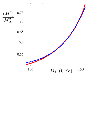
Figure 4: The average squared mass of Eq. (32), as a function of $M_{H}$, in the process $H\to WW^{*}$, for $M_{H}<1.93\mspace{1.0mu}M_{W}$. The continuous line is the leading-order calculation in the standard model. The dashed line is the approximation of Eq. (34).

VIII Details of our data analysis

We have derived singularity variables only for the signal process, not for its backgrounds, and we use the signal singularity variables to compare the distributions of MC-generated signals and backgrounds.

We present results only for the $H\to WW$, $W\to e\nu$, $W\to\mu\nu$ channel and its non-resonant $WW$ and $t\bar{t}$ backgrounds, with leptons of transverse momentum greater than 15 GeV, and satisfying the pseudorapidity cuts $\eta(e)<2.5$, $\eta(\mu)<2.1$ SMS .

Given the delicacies of measuring or simulating (at a “reconstruction level”) the transverse momentum of hadrons, $p_{T}$, we have not boosted each event to the approximate frame wherein the putative Higgs boson is transversally at rest. Our MC-simulations are for “generator level” events and do not have a $p_{T}=0$ requirement. No doubt this makes our results look somewhat weaker than they might otherwise be.

The ratios of signal to background yields are fast-varying functions of $M_{H}$. The selections made by experimentalists on the way to focus on signal events are many and are also mass-dependent. These are reasons why we shall limit ourselves to illustrating only the different shapes (and not the absolute scales) of the signal and background histograms of various singular variables.

In discussing singularity variables such as $\Sigma_{0}({\cal M})$ of Eq. (20) or $\Delta_{1}({\cal M})$ of Eq. (29), it is informative to do it not only for the correct “guess” ${\cal M}=M_{H}$, but also for incorrect ones. Naturally, the histograms for a fixed $M_{H}$ and various $\cal M$ contain precisely the same statistical information. An experimentalist using an observable such as $\Sigma_{0}$ or $\Delta_{1}$ would deal with data (with $M_{H}$ not known a priori) armed with a plethora of “diagonal” MC templates with ${\cal M}=M_{H}$, with which to compare the observed distributions.

IX Data analysis in the CM approximation

In this section we sketch a numerical analysis of the partial and complete “Higgs at rest” singularity variables derived in §V. Recall that these theoretically-obtained expressions ignore both the longitudinal and transverse momentum of the Higgs-boson signal to be analized.

IX.1 Partial singularity conditions

We start this part of the discussion with the singularity variable $\Sigma_{0}$, a measure of distance of an event to the partial singularity condition of coplanarity: $\Sigma_{0}=0$. We chose $M_{H}=500$ and 120 GeV as examples of the “true” mass of the events in this first illustration.

The distribution of values of $\Sigma_{0}$ for 20000 signal events generated with $M_{H}=500$ GeV is shown in the left panels of Fig. 5. The top left panel is for the correct assumption ${\cal{M}}=M_{H}$, the two other left panels show comparisons with the incorrect assumptions ${\cal M}=4\mspace{1.0mu}M_{H}/5$ (middle) and ${\cal M}=5\mspace{1.0mu}M_{H}/4$ (bottom). The right panels of Fig. 5 show results for $M_{H}\!=\!140$ GeV. The top panel is for the correct assumption ${\cal{M}}\!=\!M_{H}$. The middle panel is for ${\cal{M}}\!=\!120$ GeV and the lower one for ${\cal{M}}\!=\!160$ GeV. At $M_{H}\!=\!500$ GeV the distribution of $\Sigma_{0}$ is very sensitive to the boson’s mass, as exemplified in Fig. 5 by the sensitivity to ${\cal M}$. At $M_{H}\!=\!140$ GeV this is less so.

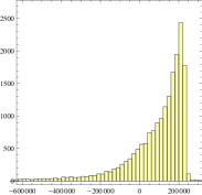
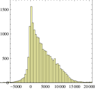
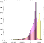
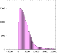
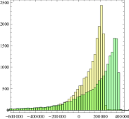
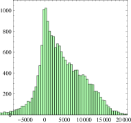
Figure 5: The distribution of $\Sigma_{0}$ values. The horizontal scales are in units of GeV². The left column in for $M_{H}=500$ GeV. Its top figure is for ${\cal{M}}=M_{H}$. In its middle (lower) ones the result is compared with that of the incorrect ${\cal{M}}=(4/5)M_{H}$ (${\cal{M}}=(5/4)M_{H}$). The right panels are for $M_{H}=140$ GeV. The top one is for the correct ${\cal{M}}=M_{H}$. The middle panel is for ${\cal{M}}=120$ GeV, the lower one for ${\cal{M}}=160$ GeV. In the figures the correct-guess histogram is yellow.

The ability of the $\Sigma_{0}$ distribution to sieve apart signal and background shapes is illustrated in Fig. 6. Its left (right) columns are for $M_{H}=500$ (120) GeV, both with ${\cal M}$ set to its corresponding correct value. The top (bottom) lines refer to the $WW$ and $t\bar{t}$ backgrounds. In all cases we have simulated equally many signal and background events, so that the figure reflects the shape of the distributions, not their relative weights. At $M_{H}=120$ GeV the shape of signal and backgrounds are very different, while at $M_{H}=500$ GeV this is less so.

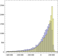
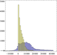
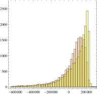
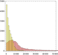
Figure 6: Shapes of the $\Sigma_{0}$ distributions for the signal –the yellow tallest histogram– and the $WW$ and $t\bar{t}$ backgrounds (upper and lower rows). The horizontal scales are in GeV² units. The left (right) column is for $M_{H}=500$ (120) GeV.

The conclusions on the ability to distinguish signal and backgrounds or different Higgs masses are, as we saw, very mass dependent. The rest of the questions to be discussed in this chapter are quite insensitive to $M_{H}$. We shall study them only for the $M_{H}=120$ GeV example.

The quantity $\Sigma_{0}$ of Eq. (20) is real, but its roots, $M_{\pm}$, need not be. For input MC data corresponding to $M_{H}=120$ GeV, about 14% of the roots are a real pair, the rest being two conjugate complex numbers. The conclusion that the complex roots are useless would be most premature. A feature of these roots to be studied ab initio is the correlation between their absolute value and phase. This is done for the $M_{H}=120$ GeV signal and the $WW$ and $t\bar{t}$ backgrounds in Fig. 7, where the mass axis is the absolute value of the roots (shown once for each complex root and for its two values for each real pair). The $\varphi$ axis is the phase of the roots having a non-negative imaginary part. We see that the $\{\varphi,|M|\}$ correlation is weak and the distributions are significantly different for signal and background.

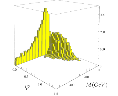
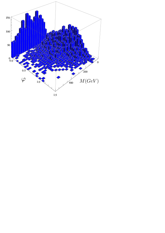
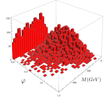
Figure 7: Correlation between absolute value $M$ and the phase $\varphi$ of the roots of $\Sigma_{0}$. Top: $M_{H}=120$ GeV signal. Middle: $WW$ background. Bottom: $t\bar{t}$ background. The real roots gather along the $\varphi=0$ axis.

The distribution of absolute values and phases of the roots of $\Sigma_{0}$, that is the projections of the results of Fig. 3 onto the $|M|$ and $\varphi$ axis, are shown in Fig. 8. The results for signal and $WW$ and $t\bar{t}$ backgrounds are significantly different. Notice in particular how the signal has a much higher fraction than the background of events with $|M|$ and $\varphi$ close to zero.

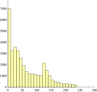
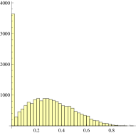
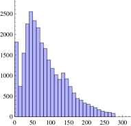
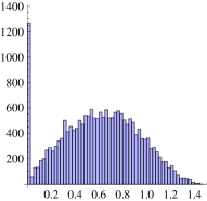
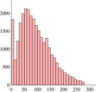
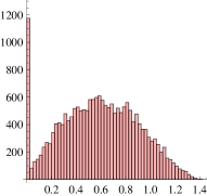
Figure 8: Shapes of the distributions of $|M|$ (left column) and $\varphi$ (right column) of the roots of $\Sigma_{0}$. The top row is the $M_{H}=120$ GeV signal. The $WW$ and $t\bar{t}$ backgrounds are shown in the middle and lower rows. $|M|$ is in GeV units.

The variables $M_{1,2}$ of Eqs. (21,22) are akin to $M_{\pm}$ in that they do not refer to an ansatz mass ${\cal M}$. In spite of their naiveté, these observables, particularly $M_{2}$, are quite good at telling signal from backgrounds. Their shapes for an $M_{H}=120$ GeV signal and the $WW$ and $t\bar{t}$ backgrounds are shown in Fig. 9.

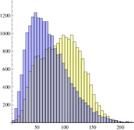
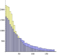
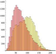
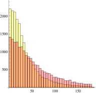
Figure 9: Comparison of the shapes of the distributions of $M_{2}$ (left column) and $M_{1}$ (right column) for an $M_{H}=120$ GeV signal (yellow) and the $WW$ (top row) and $t\bar{t}$ (lower row) backgrounds. See Eqs. (22,21). Abscissae in GeV units.

Because the variable $\Sigma_{3}$ of Eq. (23) has mass dimension 3, it is convenient to plot its sign-recalling cubic root of Eq. (24). This we do in the left column of Fig. 10 for an $M_{H}=120$ GeV signal and the $WW$ and $t\bar{t}$ backgrounds. The signal and the illustrated backgrounds are seen to result in distributions with similar looks but significantly different details. In the right column of Fig. 10 we show the three roots of the cubic equation $\Sigma_{3}({\cal M})=0$, see Eq. (23). The taller (yellow) histograms are the $M_{H}=120$ GeV signal, they are compared with those of the $WW$ background (the $t\bar{t}$ distributions, not shown, differ a bit more than the $WW$ ones from the signal distributions). The three roots $\tilde{M}_{i}$ of $\Sigma_{3}$, unlike the roots $M_{\pm}$ of $\Sigma_{0}$, are not so useful in telling signal from backgrounds.

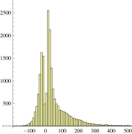
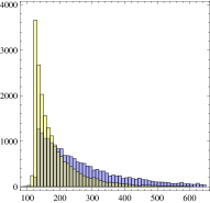
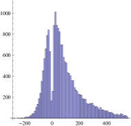
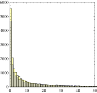
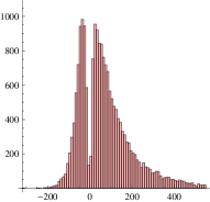
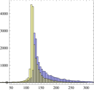
Figure 10: Left: distributions of the variable $\tilde{\Sigma}_{3}$ of Eq. (24); top is the $M_{H}=120$ GeV signal, middle is the $WW$ background, bottom is the $t\bar{t}$ one. Right: distributions of the three roots of $\Sigma_{3}({\cal M})=0$, for the quoted signal (tall and yellow) compared with the $WW$ background. Abscissae in GeV units.

IX.2 Correlations between partial singularity variables

A question of practical interest is the extent to which the $C_{0}$ and $C_{1,2,3}$ distributions of Eqs. (20,18) are correlated, for a putative signal, and for the backgrounds. It can be answered, pictorially, by contemplating 2D histograms in the three $\{C_{0},C_{i}\}$ planes. In the $\{C_{0},C_{3}\}$ case, for which the functions depend on ${\cal M}$, we choose to plot the results in the $\{\tilde{\Sigma}_{0},\tilde{\Sigma}_{3}\}$ plane, see Eqs. (20,23). The singularity, for the correct assignment ${\cal M}=M_{H}$, is at the origin of the plane. For this to be the case in the two other pairs, we plot results for $\{\tilde{\Sigma}_{0},\Sigma_{1}\}$ and $\{\tilde{\Sigma}_{0},\Sigma_{2}\}$, see Eq. (24). All this we do in Fig. (11).

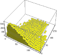
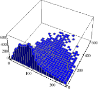
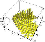
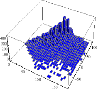
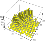
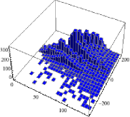
Figure 11: Top left: Histogram of the values of $\tilde{\Sigma}_{0}$ and $\Sigma_{1}$, for a signal with $M_{H}=120$ GeV. Top right: for the $WW$ background. Middle row: the same as the first row, for $\{\tilde{\Sigma}_{0},\Sigma_{2}\}$. Third row: $\{\tilde{\Sigma}_{0},\Sigma_{3}\}$. All plots are made for ${\cal M}=120$ GeV and all horizontal scales (which do not have the same extent in all figures) are in GeV units. The relevant definitions are in Eqs. (20, 23, 24).

Two conclusions are to be extracted from the quoted figure, after noticing that its horizontal scales for signal and backgrounds are not always the same. The signal variable pairs are quite correlated, with the exception of $\{\Sigma_{0},\Sigma_{1}\}$. The $WW$ background is less correlated and its distribution is significantly different from that of the signal, for all variable pairs. These statements are more so for the $t\bar{t}$ background, which we have not shown.

IX.3 Complete CM singularity conditions

To construct true singularity variables that reflect a complete set of singularity conditions we must exploit a measure of the distance between a data point (its values of $\vec{k}$ and $\vec{l}\,$) and one of the three center-of-mass singularities which, for ${\cal M}=M_{H}$, are the points $\{0,0\}$ of the planes $\{\Sigma_{0},\Sigma_{i}\}$, $i=1$ to 3. These are the quantities $D_{i}$ defined in Eqs. (25). Distributions of these variables are shown in Fig. 12. The three choices appear to be comparably efficient at telling signal from backgrounds.

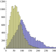
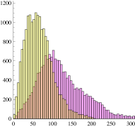
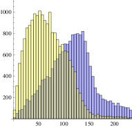
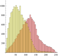
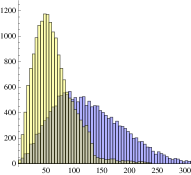
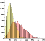
Figure 12: Histograms of the singularity variables $D_{i}$ of Eq. (25). Top: $D_{1}$. Middle: $D_{2}$. Bottom: $D_{3}$. Left: comparison of the signal for ${\cal M}=M_{H}=120$ GeV (the distribution peaking closer to zero) with the $WW$ background. Right: comparison of the same signal with the $t\bar{t}$ background. Abscissae in GeV units.

The $\{D_{i},D_{j}\}$ correlations are illustrated in Fig. 13 for a signal with $M_{H}=120$ GeV and for the $WW$ background, all with ${\cal M}=M_{H}$. Only the $\{D_{2},D_{3}\}$ correlation is strong. In all cases the signal and background results are fairly distinct. This is even more so for the $t\bar{t}$ background, results for which we do not show.

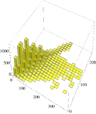
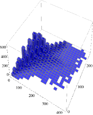
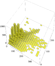
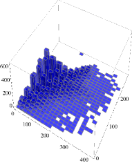
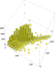
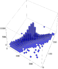
Figure 13: Histograms of the correlations between the singularity variables $D_{i}$ of Eq. (25). Left: the signal for $M_{H}=120$ GeV. Right: $WW$ background. Top: $\{D_{1},D_{2}\}$. Middle: $\{D_{1},D_{3}\}$. Bottom: $\{D_{2},D_{3}\}$. Horizontal axes is GeV units.

X Data analysis beyond the CM approximation

We have derived three longitudinally boost-invariant singularity variables. The first of them, $\Delta_{1}$ is algebraically simple and factorizable as $\Delta_{1}\!\propto\!M^{2}\,\Sigma$, see Eq. (29). The mass dimension of $C^{\prime}_{1}$ is 1 and its degree in $\xi$ is 2. The corresponding numbers for $C^{\prime}_{0}$ are 6 and 8, see Eqs. (27). The mass dimension of their resultant is $1\times 8+6\times 2=20$. The mass dimensions of $M$ and $\Sigma$ are 4 and 12, respectively. It is therefore convenient to discuss the results in terms of $M^{1/4},\,\Sigma^{1/12}$ and

$$\tilde{\Delta}_{1}\equiv\Delta_{1}^{1/20},$$ (35)

where the root is always real, since $\Delta_{1}$ is always positive.

For the quoted variables we show in Fig. 14 histograms comparing the quite distinct shapes of the distributions for a signal of a Higgs boson of mass $M_{H}=120$ GeV and the $WW$ and $t\bar{t}$ backgrounds, for ${\cal M}=M_{H}$ in the case of $\Sigma$ and $\Delta_{1}$. The distributions of $M^{1/4}$ and $\Sigma^{1/12}$ –and consequently $\tilde{\Delta}_{1}$– are similar, since the first two variables are correlated. The correlations, shown in Fig. (15), are not as strong as one might have suspected on the basis of Fig. 14 . The correlations are weaker for the signal than they are for the background, except in the high-mass tails of the background distributions.

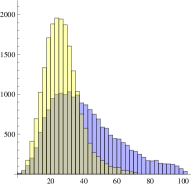
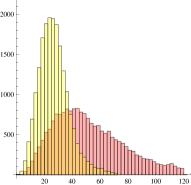
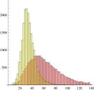
Figure 14: Histograms of the singularity variables $M^{1/4},\Sigma^{1/12}$ and $\tilde{\Delta}_{1}$ of Eq. (29). Top: $M$. Middle: $\Sigma$. Bottom: $\Delta_{1}$. Left: comparison of the shape of the signal for ${\cal M}=M_{H}=120$ GeV (the distribution peaking closer to zero) with the shape of the $WW$ background. Right: comparison of the same signal shape with that of the $t\bar{t}$ background. Abscissae in GeV units.

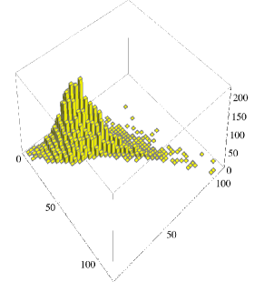
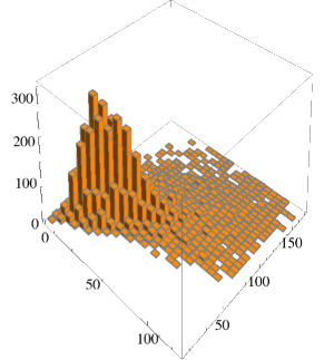
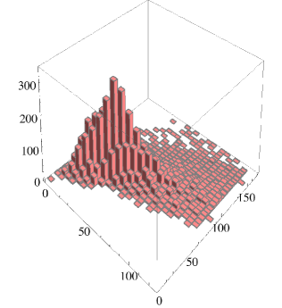
Figure 15: Correlations between $M^{1/4}$ and $\Sigma^{1/12}$. Top: The Signal for ${\cal M}=M_{H}=120$ GeV. Middle: $WW$ background. Bottom: $t\bar{t}$ background. The horizontal scales are in GeV and do not have the same extent in all figures.

The ability of $\Sigma$ and its factors to tell apart diverse masses (120 and 140 GeV in the coming instance) is studied in Fig. 16. The top left figure, histogramming $\Sigma^{1/12}$, is for a fixed $M_{H}=120$ GeV, with ${\cal M}=M_{H}$ or 140 GeV. The other tree figures, for $M^{1/4},\,\Sigma^{1/12}$ and $\tilde{\Delta}_{1}$ are for $M_{H}=120$, 140 GeV with, in all cases, ${\cal M}=M_{H}$. The function $\Sigma({\cal M})$ is quadratic in ${\cal M}$ so that its roots, in analogy with $M_{\pm}$ in Eq. (20) can be made explicit. But they are not very efficient at telling apart signal from backgrounds, nor at zooming into a value of $M_{H}$. Thus, we do not show results for them.

We conclude that the singularity variable $\Delta_{1}$ and its factors are strong boost-invariant tools to tell signal from backgrounds, and is not very stringent in constraining the value of $M_{H}$.

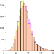
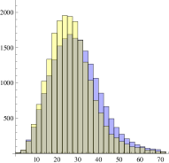
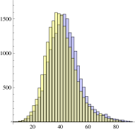
Figure 16: Top left: The distribution of $\Sigma^{1/12}$ for a signal with $M_{H}=120$ GeV. The (yellow) histogram peaking at a smaller value of $\Sigma$ is for the correct ${\cal M}=M_{H}$. The other histogram is for ${\cal M}=140$ GeV. Top right: The distribution of $M^{1/4}$ for “data” with $M_{H}=120$ and $M_{H}=140$ GeV. Bottom left: The distribution of $\Sigma^{1/12}$ for the same data, with ${\cal M}=M_{H}$ in each case. Bottom right: The same as the last entry, for $\tilde{\Delta}_{1}$. In all cases the lower-peaking histogram his for $M_{H}=120$ GeV. The horizontal scales are in GeV.

The mass dimension of $C^{\prime}_{2}$ is 3 and its degree in $\xi$ is 4. The corresponding numbers for $C^{\prime}_{0}$ are 6 and 8, see Eq. (27). Thus, the mass dimension of $\Delta_{2}\equiv{\rm Res}\{C^{\prime}_{2},C^{\prime}_{0}\}$ is $3\times 8+4\times 6=48$. In analogy with Eqs. (24), it is convenient to define

$$\tilde{\Delta}_{2}\equiv{\rm Sign}(\Delta_{2})\,|\Delta_{2}|^{1/48}$$ (36)

Results for the distributions of this singularity variable are presented in Figs. 17, 18 and commented later.

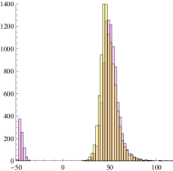
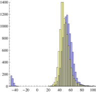
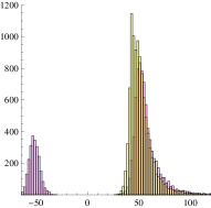
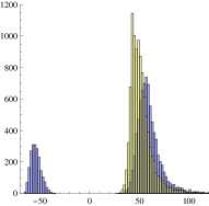
Figure 17: Study of the sensitivity to mass of $\tilde{\Delta}_{2}$, Eq. (36) (top row), and of $\tilde{\Delta}_{3}$, Eq. (37) (bottom row). The (yellow) histograms peaking at a smaller values are, in all graphs, for the correct ${\cal M}=M_{H}=120$ GeV. Left: Comparison with an incorrect choice ${\cal M}=140$ GeV. Right: Comparison with data for $M_{H}=140$ GeV, analized with the correct ${\cal M}=M_{H}$. The horizontal scale is in GeV.

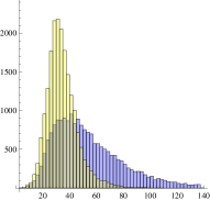
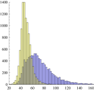
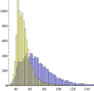
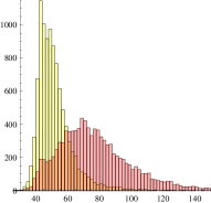
Figure 18: Signal vs $WW$ (left column) and $t\bar{t}$ backgrounds (right column) for the variables $\tilde{\Delta}_{1}$ (top row), $\tilde{\Delta}_{2}$ (middle row) and $\tilde{\Delta}_{3}$ (bottom row), respectively defined in Eqs. (35,36,37). In all graphs ${\cal M}=M_{H}=120$ GeV. The horizontal scale is in GeV.

The mass dimension of $C^{\prime}_{3}$ is 7 and its degree in $\xi$ is 12. Recall that thee corresponding numbers for $C^{\prime}_{0}$ are 6 and 8. The mass dimension of $\Delta_{3}\equiv{\rm Res}\{C^{\prime}_{3},C^{\prime}_{0}\}$ is $7\times 8+12\times 6=128$. In analogy with Eq. (36), it is thus convenient to define

$$\tilde{\Delta}_{3}\equiv{\rm Sign}(\Delta_{3})\,|\Delta_{3}|^{1/128}$$ (37)

Results for the distributions of this singularity variable are presented in Figs. 17, 18. The message of these figures is that the variables $\tilde{\Delta}_{1,2,3}$ are very good both at distinguishing signal and background events and $\tilde{\Delta}_{2,3}$ are very good at pinpointing the mass of a putative signal.

An interesting feature emerges when some of the histograms in Fig. 18 are remade with higher statistics and resolution, concerning the singularity functions $\tilde{\Delta}_{2,3}$, but not $\tilde{\Delta}_{1}$. This is shown in Fig. 19. A very clear narrow double peak shape appears for $\tilde{\Delta}_{3}$ (lower figure), and a hint of a similar structure for $\tilde{\Delta}_{2}$ (upper figure).

The peaks in Fig. 19 reflect individual roots in $\cal M$ of $\tilde{\Delta}_{2,3}({\cal M})$. The function $\tilde{\Delta}_{2}$ in Eq. (30) is, after elimination of the overall $E^{4}=({\cal M}/2)^{4}$ factor, still a polynomial of sixth degree in ${\cal M}^{2}$. The $\tilde{\Delta}_{3}({\cal M})$ resultant in Eq. (31) has an even more intractable degree in ${\cal M}^{2}$: twenty-two. Thus, their roots can only be extracted numerically event by event, a rather laborious task, which we postpone.

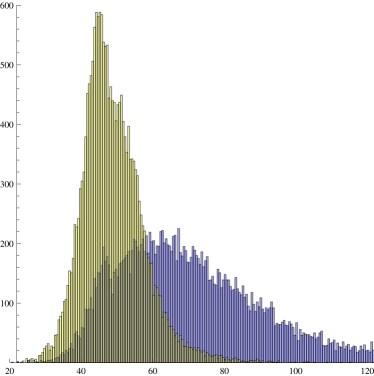
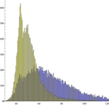
Figure 19: High resolution histograms for $\tilde{\Delta}_{2}$ (upper panel) and $\tilde{\Delta}_{3}$, showing the (narrower, yellow) signal and the (wider, blue) $WW$ background. The abscissae are in GeV units.

X.1 Correlations

The longitudinally boost invariant singularity variables $\tilde{\Delta}_{1,2,3}$ have correlations similar to the ones between $D_{1,2,3}$ that we showed in Fig. 13. They are shown in Fig. 20, for an $M_{H}=120$ GeV signal. Once again, there are significant but not extreme correlations. Moreover the correlated histograms are quite different for the signal and $WW$ background. This is even more so for the $t\bar{t}$ background, which we do not show.

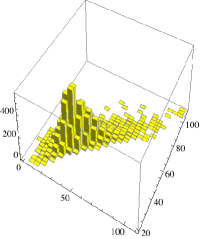
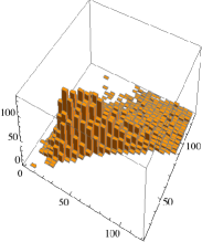
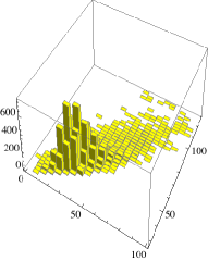
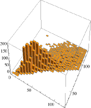
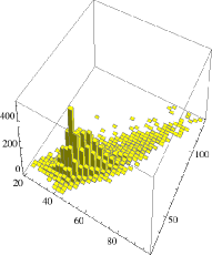
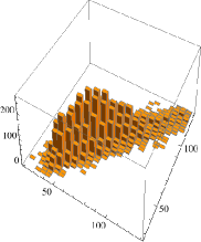
Figure 20: Histograms of the correlations between the singularity variables $\tilde{\Delta}_{i}$ of Eqs. (35,36,37). Left: The $M_{H}=120$ GeV signal. Right: $WW$ background. Top: $\{\tilde{\Delta}_{1},\tilde{\Delta}_{2}\}$. Middle: $\{\tilde{\Delta}_{1},\tilde{\Delta}_{3}\}$. Bottom: $\{\tilde{\Delta}_{2},\tilde{\Delta}_{3}\}$. The $\tilde{\Delta}_{i}$ axes are in GeV.

In Fig. 21, we illustrate the correlations between $\tilde{\Delta}_{1,2,3}$ and $\Delta\varphi$ for the signal and the $WW$ background, to which the $t\bar{t}$ background again is in this sense similar. For the relatively light $M_{H}=120$ GeV signal shown in the figure, as expected, signal and background densely populate very different regions of phase space.

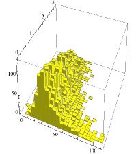
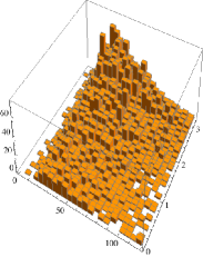
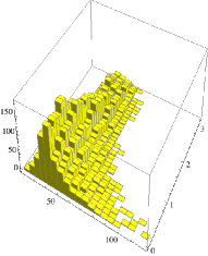
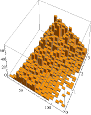
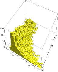
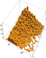
Figure 21: Histograms of the correlations between the singularity variables $\tilde{\Delta}_{i}$ of Eqs. (35,36,37) and $\Delta\varphi$. Left: The $M_{H}=120$ GeV signal. Right: $WW$ background. Top: $\{\tilde{\Delta}_{1},\Delta\varphi\}$. Middle: $\{\tilde{\Delta}_{2},\Delta\varphi\}$. Bottom: $\{\tilde{\Delta}_{3},\Delta\varphi\}$. The $\tilde{\Delta}_{i}$ axes are in GeV.

XI Summary of results

With an eye on potential practical usefulness, let us call “good” the singularity variables that do an efficient job at focusing on the correct value of $M_{H}$ and, more so, the ones that produce the most significant difference in the shape of their distributions for a potential signal and the $WW$ and $t\bar{t}$ backgrounds.

Some of the singularity variables derived in the CM approximation of a motionless Higgs boson are unexpectedly good. This is the case for $\Sigma_{0}$, associated with the CM condition of coplanarity, defined in Eq. (20) and illustrated in Figs. 5 and 6. Its two roots, $M_{\pm}$, defined in the same equation, are of the simpler kind that does not involve a trial mass $\cal M$. Their correlations, shown in Figs. 7,8 in two different ways, are moderate, both for the signal and the background. The quantities $M_{\pm}$ and their product $\Sigma_{0}^{2}({\cal M})\equiv({\cal M}-M_{+})({\cal M}-M_{-})$ are good.

Still in the CM, we see in Fig. 9 that the naïve variable $M_{1}$ (or $\Sigma_{1}$), defined in Eqs. (22,24), is not good. The variable $\Sigma_{2}\,(\tilde{\Sigma}_{3})$, also defined in Eq. (24) is good (not so good), as one can conclude from Figs. 9, 10. These limitations are lifted as we construct from these variables the quantities $D_{i}$ defined in Eq. (25), which are histogrammed in Fig. 12: they are reasonably good at telling signal from backgrounds. Their correlation plots, shown in Fig. 13, are quite disimilar for the signal and the $WW$ irreducible background.

The longitudinally boost-invariant analogs of $D_{i}$, $i=1$ to 3 are the singularity variables $\Delta_{1}$ of Eq. (29) and $\Delta_{2,3}$ of Eq. (31). We have redefined them to have unit mass dimensionality in Eqs. (35,36,37). Only for $\Delta_{1,2}$ we have analytical expressions, which are factorizable. The factors of $\Delta_{1}$, and the complete variable are very good, as illustrated in Figs. 14,15,16. So are the variables $\tilde{\Delta}_{2,3}$, as shown in Figs. 17, 18. We see in Fig. 20 that the three $\tilde{\Delta}_{i}$ are quite correlated, but the correlation plots of signal and background are populated in a significantly different way. A comparison of Fig. 18 with the corresponding result for the CM variables $D_{i}$, Fig. 12, shows, once more, that the $\tilde{\Delta}_{i}$ are demonstrably better.

The confrontation of the results for the boost-invariant variables, $\Delta_{i}$, and their siblings, $\mathord{\rm D}_{i}$, obtained in the approximation in which the boson is at rest is very gratifying. The signal peaks are significantly narrower and the correlations weaker for the $\Delta$s than for the $D$s.

In the sense of their correlations with the function $\Delta\varphi$, shown in Fig. 21, the singularity variables $\tilde{\Delta}_{i}$ are optimal tools to separate signal from backgrounds.

XII Conclusions

Recall that, as discussed in the Introduction, in the case of the CM singularity variables one can construct up to five independent combinations of the relevant observables. The best choice is the set $\{M_{+},M_{-},D_{1},D_{2},D_{3}\}$, whose ingredients are defined in Eqs. (20,25). The main appeal of these CM variables is that they are simple and explicit functions of the relevant observables. Their main drawback is that they are not as good as the boost-invariant variables, to be revisited next.

The only imperfection of the boost-invariant singularity variables is that for one of them, $\Delta_{3}$, we are unable to derive its explicit analytical expression. For $\Delta_{2}$ the analytical expression, Eq. (30), is so complex that we have opted to compute it event by event as a numerical resultant, as we are forced to do in the case of $\Delta_{3}$. For the computer, this is fast and simplest.

The practical virtues of the variables $\Delta_{i}$ –in being able to pinpoint the actual value of $M_{H}$ and to tell apart signal from backgrounds– amply overcome their quoted single limitation. The theoretical toil required to go beyond the Higgs-at-rest approximation pays.

Recall that in terms of the four boost-invariant observables one can construct up to four useful combinations. The next-to-best choice is $\{M^{1/4},\Sigma^{1/20},\tilde{\Delta}_{2},\tilde{\Delta}_{3}\}$, where $M$ and $\Sigma$ are the factors building up $\Delta_{1}$, see Eq. (29). The best choice is $\{\tilde{\Delta}_{1},\tilde{\Delta}_{2},\tilde{\Delta}_{3},\Delta\varphi\}$, combining our kinematical singularity variables with the good old “dynamical” (spin-dependent) angle, $\Delta\varphi$, of the charged leptons in the transverse plane.

The bell shapes of the signal histograms in Fig. 18 are very satisfactory, even if obtained with theoretical expressions in the $\vec{p}_{T}\!=\!0$ approximation for the produced hadrons. We have checked, by generating and analizing events with $\vec{p}_{T}\!=\!0$, that the improvement brought by theoretical variables that avoid the $\vec{p}_{T}\!=\!0$ approximation is unlikely to be very significant.

We have only studied variables and their pair-wise correlations. We have not attempted to quantify the absolute values of signals and backgrounds –as opposed to just the shape of their distributions. Thus, we are far from being able to show potential “significance” results in terms of a full multi-dimensional analysis of all variables and their correlations. Yet our results for $\tilde{\Delta}_{1,2,3}$ in Fig. 18 are competitive in “goodness” with the $\Delta\varphi$ diagnosis recalled in Fig. 1. That was one of our goals.

For an experimentalist eager to test the tantalizing hints that $M_{H}=126$ or 124 GeV LHC , it should not be too streneous to prepare the relevant one- or multi-dimensional singularity-variable templates for the relatively copious channel $H\to WW\to$ leptons.

Our main aim was the theoretical derivation of a complete set of phase-space singularity conditions and variables for the process $H\to W^{+}W^{-}$, $W^{\pm}\to\ell^{\pm}\nu$. We have seen it is a rather laborious task. The origin of its difficulty is many-fold. First, because of the elusiveness of neutrinos, the kinematical constraints of Eqs. (3) are incomplete. Second, several of these equations are non-linear. Finally and most severely, the 7-th equation, the one reflecting that the invariant mass of the four leptons is $M_{H}$, inextricably links the leptons resulting from the decay of one $W$ to those from the other, very significantly complicating the ensuing algebra.

In most processes relevant to a hadron-collider search for new physics involving unobservable particles, the initial step is a non-resonant production of a pair of novel particles. This means one cannot assume a fixed invariant mass for the pair and (approximately) boost each event to the pair’s rest system. But the last difficultly mentioned in the previous paragraph is absent. That is why, even for $\vec{p}_{T}\neq 0$ –and a surfeit of unknown masses– the pertinent singularity variables are relatively simple, and analytical AAbis .

Appendix: SO(1,1) invariance of the resultants

Let $C_{i},C_{0}$ be the CM functions defined in Eqs. (18,19). Let $C^{\prime}_{i},C^{\prime}_{0}$ be the functions in Eq. (27), boosted by $L_{\xi}\in{\rm SO}(1,1)$, whose action on a longitudinal vector $v=\{v_{0},v_{3}\}$ is $v\mapsto L_{\xi}(v)$. Very explicitly, with $\xi$ the boost parameter in Eq. (28),

$$\begin{split}&v_{0}\mapsto(L_{\xi}v)_{0}:=\frac{1}{2}(\xi+\xi^{-1})v_{0}+\frac{1}{2}(\xi-\xi^{-1})v_{3},\\ &v_{3}\mapsto(L_{\xi}v)_{3}:=\frac{1}{2}(\xi-\xi^{-1})v_{0}+\frac{1}{2}(\xi+\xi^{-1})v_{3},\end{split}$$ (38)

and

$$\begin{split}&C^{\prime}_{i}(l,k,\xi)=\xi^{r_{i}}C_{i}(L_{\xi}^{-1}l,L_{\xi}^{-1}k),\\ &C^{\prime}_{0}(l,k,\xi)=\xi^{r_{0}}C_{0}(L_{\xi}^{-1}l,L_{\xi}^{-1}k),\end{split}$$ (39)

where $r_{i},r_{0}$ are the minimal entire numbers required for $C^{\prime}_{i},C^{\prime}_{0}$ to be polynomials in $\xi$. It is easy to check that

$$\begin{split}&r_{i}=g_{i}/2,\;\;\;r_{0}=g_{0}/2,\end{split}$$ (40)

with $g_{i}$ and $g_{0}$ the degrees in $\xi$ of $C^{\prime}_{i}$ and $C^{\prime}_{0}$.

Let $R(l,k)$ be the resultant in $\xi$ of $C^{\prime}_{i}(l,k,\xi),C^{\prime}_{0}(l,k,\xi)$:

$$R(l,k):={\rm Res}(C^{\prime}_{i}(l,k,\xi),C^{\prime}_{0}(l,k,\xi),\xi).$$ (41)

We want to prove that

$$R(l,k)=R(L_{\eta}l,L_{\eta}k)$$ (42)

for all $L_{\eta}\in{\rm SO}(1,1)$, that is, the resultant is invariant under longitudinal boosts.

Indeed, using the aforementioned definitions, we have:

$$\begin{split}&R(L_{\eta}l,L_{\eta}k)={}\\ &{\rm Res}(C^{\prime}_{i}(L_{\eta}l,L_{\eta}k,\xi),C^{\prime}_{0}(L_{\eta}l,L_{\eta}k,\xi),\xi)={}\\ &{\rm Res}(\xi^{r_{i}}C_{i}(L_{\xi}^{-1}L_{\eta}l,L_{\xi}^{-1}L_{\eta}k),\xi^{r_{0}}C_{0}(L_{\xi}^{-1}L_{\eta}l,L_{\xi}^{-1}L_{\eta}k),\xi)={}\\ &{\rm Res}(\xi^{r_{i}}C_{i}(L_{\xi/\eta}^{-1}l,L_{\xi/\eta}^{-1}k),\xi^{r_{0}}C_{0}(L_{\xi/\eta}^{-1}l,L_{\xi/\eta}^{-1}k),\xi)={}\\ &{\rm Res}(\eta^{r_{i}}C^{\prime}_{i}(l,k,\xi/\eta),\eta^{r_{0}}C^{\prime}_{0}(l,k,\xi/\eta),\xi).\end{split}$$ (43)

Taking into account that, if $p_{1}(x),p_{2}(x)$ are two arbitrary polynomials of degrees $g_{1},g_{2}$, respectively,

$$\begin{split}&{\rm Res}(a_{1}p_{1}(x/b),a_{2}p_{2}(x/b),x)={}\\ &a_{1}^{g_{2}}a_{2}^{g_{1}}b^{-g_{1}g_{2}}{\rm Res}(p_{1}(x),p_{2}(x),x),\end{split}$$ (44)

it immediately follows, with use of Eqs. (40,44), that:

$$\begin{split}&{\rm Res}(\eta^{r_{i}}C^{\prime}_{i}(l,k,\xi/\eta),\eta^{r_{0}}C^{\prime}_{0}(l,k,\xi/\eta),\xi)={}\\ &{\rm Res}(C^{\prime}_{i}(l,k,\xi),C^{\prime}_{0}(l,k,\xi),\xi)=R(l,k).\end{split}$$ (45)

The desired “Q.E.D.” is simply reached by putting together Eqs. (43,45). It is also simple and gratifying, in the case of the $\Delta_{3}$ resultant that we were unable to derive explicitly, to check its boost invariance numerically.

References

- (1) The quoted numbers are from the talks of Guido Tonelli and Fabiola Gianotti at CERN on December 13th 2011. http://indico.cern.ch/conferenceDisplay.py?confId= 164890. The corresponding updated analyses are in: the ATLAS Collaboration, CERN-PH-EP-2012-019; the CMS Collaboration, CERN-PH-EP-2012-023, arXiv:submit/0412216 (2012).
- (2) CDF and D0 Collaborations, [arXiv:hep-ex/1107.5518].
- (3) LEP Electroweak Working Group, http://lepewwg.web.cern.ch/LEPEWWG/, Oct. 2011.
- (4) I.W. Kim Phys. Rev. Lett. 104:081601 (2010), arXiv:0910.1149v1.
- (5) A. De Rújula and A. Galindo, JHEP 08 (2011) 023, arXiv:1106.0396.
- (6) T. Sjostrand, S. Mrenna, and P. Skands, “PYTHIA 6.4 Physics and Manual; v6.420, tune D6T”, JHEP 05 (2006) 026, arXiv:hep-ph.0603175.
- (7) V.D. Barger, A.D. Martin and R.J.N. Phillips, Z. Phys. C 21 (1983) 99.
- (8) J. Smith, W. L. van Neerven and J. A. M. Vermaseren, Phys. Rev. Lett. 50, 1738 (1983).
- (9) N. Cabibbo and A. Maksymowicz, Phys. Rev. 137, B438 (1965) [Erratum-ibid. 168, 1926 (1968)].
- (10) M. Kalkbrener, “An upper bound on the number of monomials in the Sylvester resultant”, Proceedings of the 1993 International Symposium on Symbolic and Algebraic Computation, pp. 161-163, ACM, New York 1993.
- (11) A. De Rújula and A. Galindo, in preparation.