An alternative expression of Di Paola and Falson’s formula for stochastic dynamics

Abstract

Di Paola and Falsone’s formula is widely used in studying stochastic dynamics of nonlinear systems under Poisson white noise. In this short communication, an alternative expression is presented. Compared to Di Paola and Falsone’s original expression, the alternative one is applicable under more general condition, and shows significantly improved performance in numerical implementation. The alternative expression turns out to be a special case of the Marcus integrals.

Keywords: Stochastic dynamics; Poisson white noise; Non-Gaussian white noise; Nonlinear systems; random vibration.

1 Introduction

In the presence of random effects, dynamics of systems in engineering and science is often modeled by stochastic differential equatinos (SDEs) driven by Gaussian or non-Gaussian processes. The solutions of SDEs are often defined by Ito or Stratonovich integrals. When the excitation is parametric Gaussian white noise, Stratonovich SDEs are different from the corresponding Ito SDEs: they have an additional term, the so-called WZ correction term [13, 14]. The studies in [7, 15] attribute the extra term to the conversion from physical white noise to ideal white noise. For Poisson white noise excitation, the correction terms for converting Stratonovich SDEs into Ito SDEs are first presented by Di Paola and Falsone [3, 4]. Although some disagreement has been brought up concerning Di Paola and Falsone’s correction term in earlier days [6, 5], the Stratonovich SDEs proposed in [3, 4] have been verified extensively and are widely used to study stochastic dynamical systems under Poisson white noise excitation [16, 17, 12, 2].

The main objective of this short communication is to give an alternative expression of Di Paola and Falsone’s formula. Compared with the original one, the alternative formula is applicable under more general condition and shows better performance in numerical computation. Note that we consider only the one-dimensional cases. The conclusion can be generalized to high-dimensional cases which, however, will not be discussed in this short communication.

2 Review of Di Paola and Falsone’s formula

Consider a dynamical system governed by

$$\dot{Z}(t)=f(Z(t),t)+g(Z(t),t)\dot{C}(t),$$ (1)

where $Z$ represents the state variable, $f$ and $g$ are deterministic functions of $Z$ and $t$, $\dot{C}(t)$ is Poisson white noise expressed as

$$\dot{C}(t)=\sum_{k=1}^{N(t)}R_{k}\delta(t-t_{k}).$$ (2)

In Eq. (2), $N(t)$ is a Poisson process with intensity parameter $\lambda$, $\delta(t-t_{k})$ is a Dirac function at $t_{k}$, $R_{k}$ is a random variable representing the $k$-th impulse. The Poisson white noise $\dot{C}(t)$ is regarded as the formal derivative of some compound Poisson process $C(t)$,

$$C(t)=\sum_{k=1}^{N(t)}R_{k}U(t-t_{k}),$$ (3)

where $U$ is a the step function.

In Ito sense, (1) is often written in the form

$${\rm d}Z(t)=f(Z(t),t)\,{\rm d}t+g(Z(t),t)\,{\rm d}C(t),$$ (4)

Di Paola and Falsone suggest to interpret (1) as [3, 4]

$${\rm d}Z(t)=f(Z(t-),t)\,{\rm d}t+\sum_{j=1}^{\infty}\frac{g^{(j)}(Z(t-),t)}{j!}\,\left({\rm d}C(t)\right)^{j},$$ (5)

where

$$\begin{cases}g^{(1)}(x,t)=g(x,t),\\ g^{(j)}(x,t)=g(x,t)\frac{\partial}{\partial x}g^{(j-1)}(x,t),\quad\text{for $j\geq 2$.}\end{cases}$$ (6)

(5) is often called the Stratonovich SDE for (1) [3, 4, 16, 17]. Note that ${\rm d}C(t)=C(t)-C(t-)$, and (3) implies that

$${\rm d}C(t)=\begin{cases}0,&\text{for}\quad t\neq t_{k};\\ R_{k},&\text{for}\quad t=t_{k}.\end{cases}$$ (7)

The effectiveness of Di Paola and Falsone’s formula expressed by (5) has been verified extensively [16, 17, 12, 2].

3 Derivation of the alternative formula

Define $Y(\lambda,t)$ as

$$Y(\lambda,t)=\sum_{j=1}^{\infty}\frac{g^{(j)}(Z(t-),t)}{j!}\lambda^{j},$$ (8)

where $g^{(j)}(x,t)$ ($j=1,2,\cdots$) are defined by (6). Using the notation $Y$ defined in (8), we can write the Stratonovich SDE (5) as

$${\rm d}Z(t)=f(Z(t),t)\,{\rm d}t+Y({\rm d}C(t),t).$$ (9)

Construct an ordinary differential equation(ODE) as

$$\begin{cases}\frac{{\rm d}y(\lambda)}{{\rm d}\lambda}=g(Z(t-)+y(\lambda),t)\quad\text{for}\quad 0\leq\lambda\leq{\rm d}\,C(t),\\ y(0)=0.\end{cases}$$ (10)

We claim that $Y({\rm d}\,C(t),t)$ as defined in (8) is the solution of the above ODE (10) at $\lambda={\rm d}C(t)$. The proof is given as follows.

First, we check the existence and uniqueness of solution for (10). It is well known that if the function $g(x,t)$ is Lipschitz continuous, then the existence and uniqueness of (10) can be guaranteed. Since (8) requires the function $g(x,t)$ be analytic with respect to $x$ [3, 4], which implies Lipschitz continuity, the existence and uniqueness of the solution follows.

Take Taylor expansion of $g(Z(t-)+y(\lambda,t),t)$ at $\lambda=0$, then (10) becomes

$$\frac{{\rm d}\,y(\lambda)}{{\rm d}\,\lambda}=g(z(\lambda),t)\big{|}_{\lambda=0}+\sum_{k=1}^{\infty}\frac{\partial^{k}}{\partial\lambda^{k}}g(z(\lambda),t)\bigg{|}_{\lambda=0}\frac{\lambda^{k}}{k!},$$ (11)

where

$$z(\lambda)=Z(t-)+y(\lambda).$$ (12)

In the following, we show by induction that

$$\frac{\partial^{k}}{\partial\lambda^{k}}g(z(\lambda),t)=g^{(k+1)}(z(\lambda),t),\quad\text{for}\quad k\geq 1.$$ (13)

For $k=1$, we obtain from (12) and (10) that

$$\frac{\partial}{\partial\lambda}g(z(\lambda),t) =\left(\frac{{\rm d}}{{\rm d}\,\lambda}z(\lambda)\right)\left(\frac{\partial}{\partial z(\lambda)}g(z(\lambda),t))\right)$$

$$=\left(\frac{{\rm d}}{{\rm d}\,\lambda}y(\lambda)\right)\left(\frac{\partial}{\partial z(\lambda)}g(z(\lambda),t))\right)$$

$$=g(z(\lambda),t))\left(\frac{\partial}{\partial z(\lambda)}g(z(\lambda),t))\right)$$

$$=g^{(2)}(z(\lambda),t)),$$ (14)

which means that (13) is true for $k=1$.

Suppose (13) is true for $k=n$, i.e.,

$$\frac{\partial^{n}}{\partial\lambda^{n}}g(z(\lambda),t)=g^{(n+1)}(z(\lambda),t)),$$ (15)

then we get

$$\frac{\partial^{n+1}}{\partial\lambda^{n+1}}g(z(\lambda),t) =\frac{\partial}{\partial\lambda}\left(\frac{\partial^{n}}{\partial\lambda^{n}}g(z(\lambda,t))\right)$$

$$=\frac{\partial}{\partial\lambda}g^{(n+1)}(z(\lambda),t))$$

$$=\left(\frac{{\rm d}}{{\rm d}\,\lambda}z(\lambda)\right)\left(\frac{\partial}{\partial z(\lambda)}g^{(n+1)}(z(\lambda),t))\right)$$

$$=g(z(\lambda),t))\left(\frac{\partial}{\partial z(\lambda)}g^{(n+1)}(z(\lambda),t))\right)$$

$$=g^{(n+2)}(z(\lambda),t)),$$ (16)

which means that (13) is also true for $k=n+1$. Now the proof of (13) is complete.

Substituting (13) into (11), and using the fact that

$$g^{(n+1)}(z(\lambda),t))\big{|}_{\lambda=0}=g^{(n+1)}(Z(t-),t)),$$ (17)

we get

$$\frac{{\rm d}\,y(\lambda)}{{\rm d}\,\lambda}=\sum_{k=1}^{\infty}g^{(k)}(Z(t-),t)\frac{\lambda^{k-1}}{(k-1)!}.$$ (18)

Integrating from $0$ to $\lambda$ at both sides of (18), we get

$$y(\lambda)=\sum_{k=1}^{\infty}g^{(k)}(Z(t-),t)\frac{\lambda^{k}}{k!}\;.$$ (19)

Comparing (19) with (8), we see the equivalence

$$Y({\rm d}C(t),t)=y({\rm d}C(t)),$$ (20)

where the right-hand side $y({\rm d}C(t))$ is the solution of the initial value problem (10) at $\lambda={\rm d}C(t)$. In other words, we obtain an equivalent and alternative expression for the Stratonovich SDE (5) or (9)

$${\rm d}Z(t)=f(Z(t),t)\,{\rm d}t+y({\rm d}C(t)),$$ (21)

where $y({\rm d}C(t))$ is the solution of the ODE (10) at $\lambda={\rm d}C(t)$.

4 Some remark and examples

As shown in section $3$, when $g(x,t)$ is analytic, $Y({\rm d}C(t),t)$ defined in (8) is equivalent to $y({\rm d}C(t))$ obtained from the ODE (10), i.e., the two forms of SDEs, (5) and (21) are equivalent. However, compared with (5), (21) has significant advantages in the following aspects.

First, for a given $g(x,t)$, one immediate advantage of the alternative expression (21) over (5) is that it is much easier to obtain analytical solution from the ODE (10) than finding the sum of the infinite Taylor series in (5). Second, the proposed alternative expression (21) is applicable under much more general condition than the original one (5). For example, when $g(x,t)$ is only continuous or piecewise continuous rather than analytic, (21) is still valid while (5) fails to exist. More importantly, the new expression (21) could have significantly improved performance in numerical implementation than the original expression (5). The form in (8) is actually the Taylor expansion of the solution of (10), which requires computing the high-order derivatives of the function $g(x,t)$ and possibly take a large number of terms to achieve high accuracy. However, since the alternative form (21) is given in form of ODE, it can be solved by numerous algorithms such as Runge-Kutta or multistep methods, which could have much better convergence and stability properties than Taylor expansion methods. The readers are referred to any numerical analysis book such as [8] for more details about the Runge-Kutta, multistep, or Taylor expansion methods for solving ordinary differential equations numerically.

We note that the alternative expression, as given in (21), turns out to be a special case of the Marcus integrals, which have been defined for general semimartingale with jumps. For more details about the Marcus integral and its application, readers are referred to [10, 11, 9, 1].

Example
In this example, $f(x,t)$ and $g(x,t)x$ are chosen such that the analytical solution of the SDE is available to compare with the numerical results.

Take $f(x,t)=x$, and $g(x,t)=x$, the SDE (5) becomes

$${\rm d}Z(t)=Z(t){\rm d}t+Y({\rm d}C(t)),$$ (22)

where $Y({\rm d}C(t))$ is expressed, by Di Paola and Falsone’s formula, as

$$Y({\rm d}C(t),t))=Z(t-)\sum_{k=1}^{\infty}\frac{\left({\rm d}C(t)\right)^{k}}{k!},$$ (23)

or by the alternative expression, as the solution of the following ODE at $\lambda={\rm d}C(t)$,

$$\begin{cases}\frac{{\rm d}y(\lambda)}{{\rm d}\lambda}=Z(t-)+y(\lambda)\quad\text{for}\quad 0\leq\lambda\leq{\rm d}\,C(t),\\ y(0)=0.\end{cases}$$ (24)

It is easy to check that the theoretical solution of (22) is $e^{t+C(t)}$.

In the simulation, the compound Poisson process $C(t)$ is taken as

$$C(t)=\sum_{k=1}^{N(t)}R_{k}U(t-t_{k}).$$ (25)

wher $N(t)$ is a Poisson process with intensity parameter as $10$ and $R_{k}$ ($k=1,\cdots,N(t)$) are normally distributed random numbers independent of each other.

When no jumps occur, $Y({\rm d}C(t))=0$ and We solve (22) by second order Runge-Kutta method with time step as $0.01$. We compute the jump of the solution $Z(t)$ by Di Paola and Falsone’s formula and the alternative formula, respectively. For the former, we truncate the infinite consequence by taking the first $6$ terms, and for the latter, we solve ODE (24) numerically by uisng second order Runge-Kuta method with step size equal to $0.1$. Figure 1 shows one random path of the Poisson compound process, and Figure 2 compares the corresponding computational results with the theoretical one. It can be seen from Fig. 2 that when the jumps are computed by the alternative formula, the numerical result agrees very well with the theoretical one. However, when using Di Paola and Falsone’s formula, the numerical result deviates from the theoretical one significantly, especially when the jump size is relatively large. We note that the accuracy for Di Paola and Falsone’s formula could be improved by keeping more terms when truncating the infinite series. However, the number of terms needed to achieve the desired accuracy with Di Paola and Falsone’s formula is not easy to predict. The alternative formula is preferred partly because its accuracy can be easily controlled by the step size and the order the Runge-Kutta or other methods.

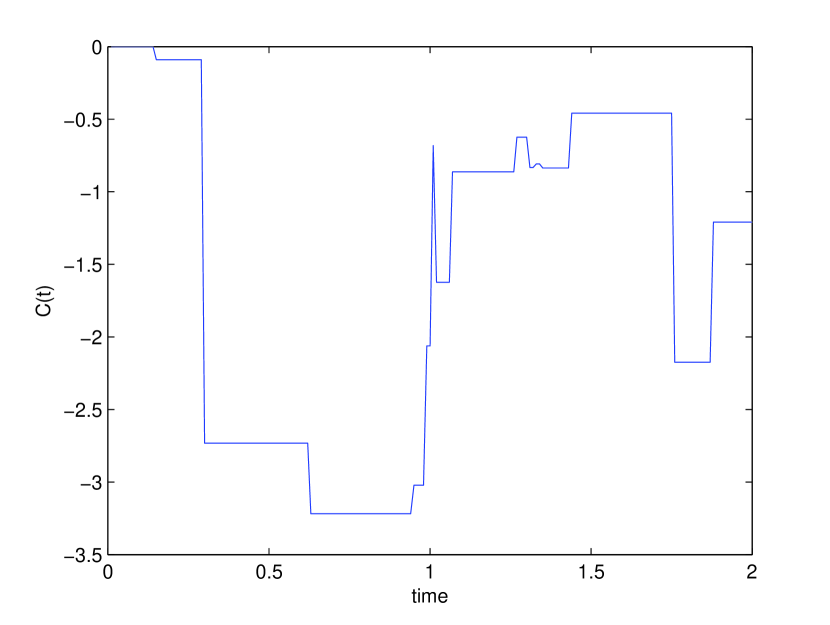
Figure 1: One random path of the driving process

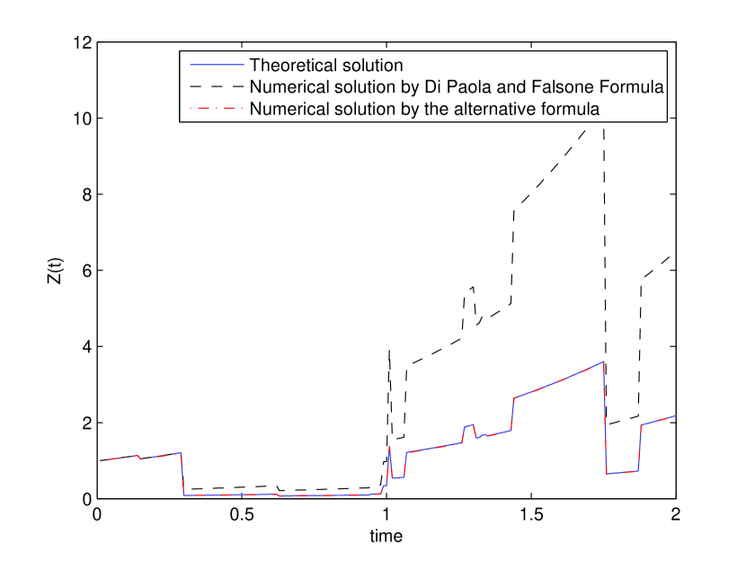
Figure 2: Comparison of the numerical results with the theoretical one

References

- [1] D. Applebaum. Levy Processes and stochastic calculus. Cambridge University Press, 2nd Edition, 2009.
- [2] S. Caddemi and M. Di Paola. Ideal and physical white noise in stochastic analysis. International Journal of Non-linear Mechanics, 31(5):581–590, 1996.
- [3] M. Di Paola and G. Falsone. Ito and stratonovich integrals for delta-correlated processes. Probabilistic engineering mechanics, 8, 1993.
- [4] M. Di Paola and G. Falsone. Stochastic dynamics of non-linear systems driven by non-normal delta-correlated processes. ASME Journal of applied mechanics, 60:141–148, 1993.
- [5] M. Grigoriu. The ito and stratonovich integrals for stochastic differential equations with poisson white noise. Probabilistic engineering mechanics, 13:175–182, 1998.
- [6] S. L. J. Hu. Closure on discussion by di paola, m. and falsone, g., on ”response of dynamic systems excited by non-gaussian pulse processes”. ASCE Journal of engineering mechanics, 120:2472–2474, 1994.
- [7] R. A. Ibrahim. Parametric Random Vibration. Research Studies Press, 1985.
- [8] D. Kincaid and W. Cheney. Numerical analysis: Mathematics of scientific computing. Brooks/Cole, 2002.
- [9] T. Kurtz, E. Pardoux, and P. Protter. Stratonovich stochastic differential equations driven by general martingales. Ann. Inst. Henri Poincare Prob. Stat., 31:351–377, 1995.
- [10] S. I. Marcus. Modeling and analysis of stochastic differential equations driven by point processes. IEEE Transanctions on information theory, IT-24:164–172, 1978.
- [11] S. I. Marcus. Modeling and approximation of stochastic differential equations driven by semimartingales. stochastics, 4:223–245, 1981.
- [12] C. Proppe. The wong-zakai theorem for dynamical systems with parametric poisson white noise excitation. International Journal of Engineering science, 40:1165–1178, 2003.
- [13] C. W. S. To. Nonlinear random vibration: Analytical techniques and applications. Swets and Zeitlinger Publishers, 2000.
- [14] E. Wong and M. Zakai. On the relation between ordinary and stochastic differential equations. International Journal of Engineering Science, 3:213–229, 1965.
- [15] Y. Yong and Y. K. Lin. Exact stationary response solution for second order nonlinear systems under parametric and external white noise excitations. Journal of Applied Mechanics, Transactions of the American Society of Mechanical Engineers, 54:414–418, 1987.
- [16] Y. Zheng and W. Q. Zhu. Stochastic averaging of quasi-linear systems driven by poisson white noise. Probabilistic engineering mechanics, 25:99–107, 2010.
- [17] Y. Zheng and W. Q. Zhu. Stochastic averaging of strongly nonlinear oscillators under poisson white noise excitation. IUTAM symposium on nonlinear stochastic dynamics and control, pages 147–155, 2010.