Degeneracy and ordering of the non-coplanar phase of the classical bilinear-biquadratic Heisenberg model on the triangular lattice

Abstract

We investigate the zero-temperature behavior of the classical Heisenberg model on the triangular lattice in which the competition between exchange interactions of different orders favors a relative angle between neighboring spins $\Phi\in(0,2\pi/3)$. In this situation, the ground states are noncoplanar and have an infinite discrete degeneracy. In the generic case, i.e. when $\Phi\neq\pi/2,\arccos(-1/3)$, the ground state manifold is in one to one correspondence (up to a global rotation) with the set of non-crossing loop coverings of the three equivalent honeycomb sublattices into which the bonds of the triangular lattice can be partitioned. This allows one to identify the order parameter space as an infinite Cayley tree with coordination number 3. Building on the duality between a similar loop model and the ferromagnetic O(3) model on the honeycomb lattice, we argue that a typical ground state should have long-range order in terms of spin orientation. This conclusion is further supported by the comparison with the four-state antiferromagnetic Potts model [describing the $\Phi=\arccos(-1/3)$ case], which at zero temperature is critical and in terms of the solid-on-solid representation is located exactly at the point of roughening transition. At $\Phi\neq\arccos(-1/3)$ an additional constraint appears, whose presence drives the system into an ordered phase (unless $\Phi=\pi/2$, when another constraint is removed and the model becomes trivially exactly solvable).

I Introduction

The recent discovery of the compound NiGaS₄, and the suggestion that it might be a spin liquid or a spin nematic, nakatsuji has revived the interest in the Heisenberg model with bilinear and biquadratic interactions defined by the Hamiltonian

$$\mathcal{H}=\sum_{(jj^{\prime})}J_{1}{\bf S}_{j}\cdot{\bf S}_{j^{\prime}}+J_{2}\left({\bf S}_{j}\cdot{\bf S}_{j^{\prime}}\right)^{2}\;,$$ (1)

where $({j}{j}^{\prime})$ stands for nearest neighbor pairs on a lattice. In one dimension, the spin-1 case has been very thoroughly investigated following Haldane’s prediction that the pure Heisenberg model is gapped,haldane and a rather complete picture of its properties has emerged both in zero (see e.g. Refs. [PRL_AKLT, ; fath1991, ; Schollwock1996, ] and references therein) and in finite magnetic field.parkinson ; okunishi1 ; fath ; manmana

In two dimensions, most of the attention has also been devoted to the spin-1 case, and some trends have emerged from the investigation of this model on the triangular and square lattices. kawashima ; arikawa ; LMP ; toth With the standard notation $J_{1}=J\cos\theta$, $J_{2}=J\sin\theta$, the phase diagram as a function of $\theta$ consists of four main phases: an antiferromagnetic phase (with two sublattices on the square lattice and three sublattices on the triangular lattice) around $\theta=0$, followed counter-clockwise by a three-sublattice antiferroquadrupolar phase up to $\theta=\pi/2$, a ferromagnetic phase around $\theta=\pi$, and finally a ferroquadrupolar phase that persists until the antiferromagnetic order sets in.

In comparison, little attention has been paid to the classical limit, where spins are classical vectors of length $1$. The main reason lies in the fact that, unlike for spin-1/2 models, in the spin-1 case the classical limit is not equivalent to the Hartree approximation (in which the ground state is approximated by a product of local wave functions) since local wave functions are not necessarily purely magnetic but can also describe quadrupolar states.

In the classical limit, the most unusual feature introduced by the presence of the biquadratic exchange is the possibility (realized in the parameter range $-2J_{2}<J_{1}<2J_{2}$ with $J_{2}>0$) to have the minimum of the interaction of two spins in a noncollinear configuration in which they make an angle

$$\Phi=\arccos\left(-\frac{J_{1}}{2J_{2}}\right)\in(0,\pi)$$ (2)

with respect to each other, while the overall orientation of the spins is arbitrary. LGT ; KY Such an interaction may be called a rotationally invariant spin-canting interaction. It should not be confused with the Dzyaloshinskii-Moriya interaction, which also induces a canting between a pair of spins but forces them to lie in a specific plane.

Note that the physics will be essentially the same for any rotationally invariant canting interaction between pairs of spins that leads to the same angle $\Phi$, for instance interactions that include higher powers of ${\bf S}_{j}\cdot{\bf S}_{j^{\prime}}$, in which case the relation (2) would have to be replaced by a more complex one. For this reason we prefer below to characterize the interaction in terms of the angle $\Phi$ and not in terms of the parameter $\theta$. The classical XY model with rotationally invariant spin-canting interaction on the square lattice has been investigated by Lee et al. LGT and the classical Heisenberg model on the triangular lattice by Kawamura and Yamamoto. KY

According to Ref. KY, , the zero-temperature phase diagram of the classical version of model 1 on the triangular lattice includes four phases (see Fig. 1): a ferromagnetic phase for $\pi-\arctan(1/2)<\theta<3\pi/2$, a nematic-like phase with collinear orientation of spins for $-\pi/2<\theta<-\arctan(2/9)$, a three-sublattice antiferromagnetic phase for $-\arctan(2/9)<\theta<\pi/4$, and a phase with non-coplanar orientations of spins for $\pi/4<\theta<\pi-\arctan(1/2)$. This phase diagram is reminiscent of the spin-1 phase diagram, but the non-degenerate ferro- and antiferroquadrupolar phases of the spin-1 case are replaced by highly degenerate magnetic phases. The nematic-like phase is thoroughly discussed in Ref. KY, , with the conclusion that it has the same degeneracy and correlations as the antiferromagnetic Ising model on the triangular lattice.

 

Figure 1: Phase diagram of the classical bilinear-biquadratic Heisenberg model on the triangular lattice.

The discussion of the non-coplanar phase is much more sketchy however. The authors point out that there is a degeneracy due to the two possible chiralities of a local umbrella [formed on each triangular plaquette when $\Phi\in(0,2\pi/3)$], but no attempt has been made to identify the structure of the ground state manifold or to study the consequences of the degeneracy on the spin correlations in a typical ground state. In the present paper, we construct the complete classification of the ground states which allows us to conclude that the non-coplanar phase is a non-trivial one even at zero temperature because the total number of ground states grows exponentially with the area of the system, as in various versions of the antiferromagnetic (AF) Potts model and other frustrated models with a finite residual entropy per site. Suto ; KB ; St ; B70 ; HR ; KSS In situations like this, it is not evident a priori whether the degeneracy leads at zero temperature to the disordering of the system or to an algebraic decay of correlations, or whether long-range order is nevertheless present.

Interestingly enough, in the two-dimensional antiferromagnets known to have an extensive residual entropy, all three scenarios are realized. In particular, both the AF Ising model on the kagomé lattice Suto and the three-state AF Potts model on the square lattice KB at zero temperature are disordered, the AF Ising model on the triangular lattice St and the three-state AF Potts model on the kagomé lattice B70 ; HR are critical, whereas the three-state AF Potts model on the dice lattice has a genuine long-range order. KSS The main aim of our paper is to establish which of the three scenarios is realized in the present case.

The paper is organized as follows. Sec. II is devoted to a complete classification of the ground states of the model in terms of the nonintersecting closed loops living on the bonds of the triangular lattice, which allows us to redefine the problem as a loop model. In Sec. III we show that the order-parameter manifold of this loop model has the same topology as that of the $O(n)$ model with $n=3$, which suggests that they belong to the same universality class and, therefore, that both of them are in the ordered phase. In Sec. IV, the same conclusion is confirmed by establishing a relation with the four-state AF Potts model on the same lattice and by relying on some known properties of this Potts model. For completeness, Sec. V briefly discusses the case $\Phi=\pi/2$, where the model is trivially exactly solvable, and Sec. VI summarizes the results. Appendix A is devoted to the analysis of a simplified problem corresponding to freezing the spins on one of the three sublattices in a perfectly ordered state. It also includes estimates from below and from above of the residual entropy of the full problem.

II Ground state classification and loop model

We assume that classical spins ${\bf S}_{j}$ (three-dimensional vectors of unit length) are located at the sites ${j}$ of the triangular lattice and that the energy of the interaction of two neighboring spins $E({\bf S},{\bf S}^{\prime})$ depends only on the angle between ${\bf S}$ and ${\bf S}^{\prime}$ and is minimal when this angle is equal to $\Phi\in(0,2\pi/3)$. In terms of the coupling constants $J_{1}$ and $J_{2}$ introduced in Eq. (1) this corresponds to $-2J_{2}<J_{1}<J_{2}$ (see Eq. 2). For such values of $\Phi$, it turns out to be possible to minimize $E({\bf S}_{j},{\bf S}_{j^{\prime}})$ simultaneously for all pairs of neighboring spins $({jj}^{\prime})$, which means that the system is not frustrated. However, as we shall see, it is very highly degenerate.

The simplest ground states of the model can be constructed by choosing three unit vectors ${\bf S}^{A}$, ${\bf S}^{B}$ and ${\bf S}^{C}$ which form angles $\Phi$ with respect to each other. After that, one can partition the triangular lattice into three triangular sublattices (denoted below A, B, and C) and set all spins on sublattice A to ${\bf S}^{A}$, on sublattice B to ${\bf S}^{B}$ and on the third one to ${\bf S}^{C}$. In such a way, one obtains a periodic ground state which has a three-sublattice structure. KY Below we call such ground states regular states.

The family of regular states is characterized by an $SO(3)\times Z_{2}$ degeneracy, where the group $SO(3)$ is related to the possibility of simultaneously rotating all spins and the group $Z_{2}$ to the possibility of choosing the sign of the mixed product of the three spins located in the corners of a given plaquette to be either positive or negative. However, it is clear that the family of ground states is much wider than the set of regular states, and that, in addition to these two symmetry-induced degeneracies, it possesses also an infinite set of discrete degeneracies not related to global symmetries. Indeed, for any pair of spins ${\bf S}^{A}$ and ${\bf S}^{B}$ forming an angle $\Phi\in(0,2\pi/3)$ with respect to each other there are always two possibilities to choose the orientation of the third spin in such a way that it forms the same angle $\Phi$ both with ${\bf S}^{A}$ and with ${\bf S}^{B}$. These two orientations are mirror images of each other with respect to the plane formed by ${\bf S}^{A}$ and ${\bf S}^{B}$. Since in a regular state all plaquettes contain the same triad of spins (${\bf S}^{A}$, ${\bf S}^{B}$ and ${\bf S}^{C}$), it is clear that in such a state one can always flip an arbitrary spin into its mirror image without increasing the energy of the system.

Flipping one spin leads to a new ground state in which six neighboring triangular plaquettes (surrounding the flipped spin) form a domain of a different regular state. In order to obtain a larger domain, one has to flip other spins belonging to the same sublattice. As soon as a domain of another regular state is sufficiently large, a new domain can be formed inside it by flipping spins belonging to another sublattice, and so on.

A convenient method of describing the full set of ground states is based on the notion of a zero-energy domain wall. K86 In the system under consideration, a zero-energy domain wall can be defined as a line passing through the bonds of the triangular lattice in such a way that each segment of this line separates two plaquettes corresponding to different regular states. This means that each segment of such a wall separates two unparallel spins which on the original triangular lattice are next-to-nearest neighbors and therefore belong to the same sublattice. Then it is clear that the spin configuration in a ground state is uniquely defined as soon as one specifies the orientations of three spins on an arbitrary plaquette and the positions of all zero-energy domain walls. For brevity, in the following we simply call these objects domain walls.

By definition, a regular state contains no domain walls, whereas flipping of a single spin leads to the formation of the simplest closed domain wall consisting of six segments joining each other at angle $2\pi/3$, i.e. a hexagon. By flipping a larger number of spins belonging to the same sublattice one can construct more complex domain walls. However, it is clear that any wall has to be closed (or end at the boundary) and its neighboring segments always have to form angles of $\pm 2\pi/3$ with respect to each other, as in Fig. 2(b).

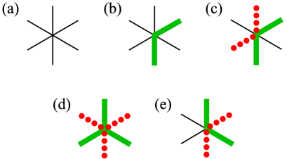
Figure 2: (Color online) The loop representation: (a)-(c) allowed configurations of loops, (d) additional vertex allowed only at $\Phi=\arccos(-1/3)$, (e) the vertex corresponding to an intersection of loops (allowed only at $\Phi=\pi/2$). The domain walls on different sublattices are shown with lines of different types.

Since each domain wall can be associated with spin-flipping on a particular sublattice of the triangular lattice, all domain walls can be partitioned into three classes (which below are called colors). The domain walls of a given color live on one of the three equivalent honeycomb sublattices into which the bonds of the triangular lattice can be partitioned. Therefore, just by construction walls of the same color have no possibility of crossing or touching each other.

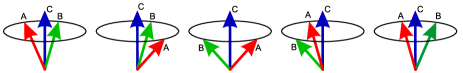
Figure 3: (Color online) From left to right, configurations obtained after successive flips of spins A, B, A, B. In the final configuration, the triad of spins is rotated around C by an angle $4\Psi(\Phi)$ with respect to the original one.

A less evident property is that for a generic value of $\Phi$ walls of different colors are also unable to cross each other. This is so because when going around an intersection of two walls [see Fig. 2(e)] one has to perform successive spin flips on sublattice $\alpha$ (where $\alpha=A,B,C$), then on another sublattice $\beta$ and once again on $\alpha$ and then on $\beta$, and return after that to the same configuration. At a formal level, this corresponds to the fulfillment of the condition

$$(\hat{R}_{\beta}\hat{R}_{\alpha})^{2}=1\,,$$ (3)

where $\hat{R}_{\alpha}$ denotes the operation of spin-flipping on sublattice $\alpha$ ($\hat{R}^{2}_{\alpha}\equiv 1$). However, since each of the operators $\hat{R}_{\alpha}$ and $\hat{R}_{\beta}$ involves a rotation of a spin around the third spin of the triad by the angle $2\Psi(\Phi)$, where

$$\Psi(\Phi)=\arccos\left(\frac{\cos\Phi}{1+\cos\Phi}\right)\in\left(\pi/3,\pi\right),$$ (4)

the application of $(\hat{R}_{\beta}\hat{R}_{\alpha})^{2}$ rotates the whole configuration by $4\Psi(\Phi)$. It is easy to check that one returns to the initial configuration only for $\Phi=\pi/2$ (when $\Psi$ is also equal to $\pi/2$), whereas for all other values of $\Phi$ the operator $(\hat{R}_{\beta}\hat{R}_{\alpha})^{2}$ brings a triad of spins into a configuration rotated with respect to the original one, as illustrated in Fig. 3.

Condition (3) can be also rewritten as $\hat{R}_{\alpha}\hat{R}_{\beta}=\hat{R}_{\beta}\hat{R}_{\alpha}$, which means that the zero-energy domain walls can cross each other only when operators $\hat{R}_{\alpha}$ commute with each other. However, walls of different colors can touch each other, as shown in Fig. 2(c).

As a consequence of the rules discussed above, for each site of the triangular lattice there are only three possibilities: (i) the absence of any domain wall passing through this site [see Fig. 2(a)], (ii) the presence of a single domain wall whose segments form an angle $2\pi/3$ with each other [see Fig. 2(b)] and (iii) the presence of two domain walls touching each other [see Fig. 2(c)]. Therefore, to understand the zero-temperature properties of the system, one has to study a loop model on the triangular lattice in which on each site only the configurations shown in Figs. 2(a)-(c) are allowed (as well of course as those that can be obtained from them by rotation), whereas all other configurations are prohibited [for example, the intersection of two domain walls shown in Fig. 2(e)]. The two exceptions where other configurations of zero-energy domain walls are allowed are the cases $\Phi=\arccos(-1/3)$ and $\Phi=\pi/2$, discussed respectively in Sec. IV and Sec. V.

One can introduce on each triangular plaquette $k$ a binary variable $\chi_{k}=\pm 1$ defined in such a way that it is perfectly ordered in any regular ground state and changes its sign on crossing each domain wall. In terms of the original spin variables ${\bf S}_{j}$ the value of $\chi_{k}$ is given by the sign of the mixed product ${\bf S}_{{j}_{A}(k)}\cdot[{\bf S}_{{j}_{B}({k})}\times{\bf S}_{{j}_{C}({k})}]$, where the three sites ${j}_{A}({k})$, ${j}_{B}({k})$ and ${j}_{C}({k})$ belonging to plaquette ${k}$ are labelled after the sublattice to which they belong. Below for simplicity we call variable $\chi_{k}$ chirality of plaquette ${k}$, although more accurately it should be called staggered chirality.

III Order-parameter manifold

Let us define neighboring regular states as regular states which can be transformed into each other by flipping the spins of one of the three sublattices. From the definition of a domain wall it is clear that in any ground state the domains lying on both sides of any domain wall belong to neighboring regular states. Since each regular state has exactly three neighboring states, at zero temperature the order-parameter manifold of our system has the topology of an infinite Cayley tree (also known as Bethe lattice) with coordination number $n=3$. Each node of this tree represents a regular ground state, while the links connect neighboring states. If one ascribes to each link on the tree the color of the corresponding domain wall, the three links connecting any node with its neighbors will all be of different colors.

Fig. 4 illustrates the correspondence between the domains of various regular states and the nodes of the Cayley tree whose links are colored in such a way. On the top panel, the domains corresponding to the same regular state are marked by the same number (the numbering being arbitrary). On the bottom panel, the same set of numbers is used to mark the nodes of the Cayley tree. The distance on the tree corresponds to the minimal number of spin flips one has to make (in other terms, the minimal number of domain walls one has to cross) to get from one regular state to another.

The tree-like topology of the order-parameter manifold (that is, the absence of closed loops) is ensured by the impossibility (for a generic value of $\Phi$) to return to the same state after crossing a sequence of domain walls corresponding to a product of operators $\hat{R}_{\alpha}$ which cannot be reduced to unity by application of the identity ${\hat{R}}_{\alpha}^{2}=1$. This property follows from the fact that intersections of domain walls are not allowed.

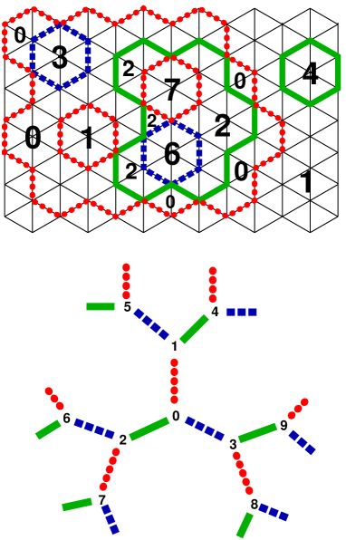
Figure 4: (Color online) Top panel: Example of loop covering. The numbers refer to the positions of different domains on the Cayley tree shown in the lower panel. The numbering is arbitrary and has been included to keep track of the relative positions on the tree.

Another model with the same structure of the order-parameter manifold is obtained when one considers a loop model on the honeycomb lattice DMNS ; Nienh in which each closed loop of length $L$ is ascribed a factor

$$w(L)=nK^{L}\,.$$ (5)

In this model the loops cannot intersect or touch each other simply because the geometry of the honeycomb lattice does not allow for this. The number $n$ can then be interpreted as the number of different colors the loops can have. This allows one to interpret these colored loops as domain walls DMNS separating the states on a Cayley tree with coordination number $n$ by following the same rule that the states separated by a domain wall of a given color correspond to neighboring nodes connected by a link of the same color.

For $n=3$ the only difference between the two models is that in our model the loops of different colors are living on three different (interpenetrating) honeycomb lattices, whereas in the loop model of Ref. DMNS, they are living on the same honeycomb lattice. However in both models the loops cannot cross each other or have an overlap, which ensures that the two models have the same order-parameter manifold and therefore can be expected to belong to the same universality class.

In Ref. DMNS, it has been shown that the loop model defined by Eq. (5) is a dual representation of a ferromagnetic $O(n)$ model whose partition function can be written as

$$Z_{O(n)}=\mbox{Tr}\left[\prod_{({kk^{\prime}})}\left(1+K{\bf s}_{k}{\bf s}_{k^{\prime}}\right)\right]\,,$$ (6)

where ${\bf s}_{k}$ are $n$-dimensional unit vectors defined at the sites ${k}$ of the honeycomb lattice, the product is taken over all bonds $({kk^{\prime}})$ of this lattice and the trace implies the unweighted integration over all variables ${\bf s}_{k}$. On the other hand, it is also well known that in $O(n)$ models with $n>2$ the long range order in ${\bf s}_{k}$ is always destroyed by small continuous fluctuations of the order parameter (the spin waves), Pol which leads to an exponential decay of the correlation functions $\langle{\bf s}_{k_{1}}{\bf s}_{k_{2}}\rangle$ with the distance between ${k}_{1}$ and ${k}_{2}$.

It follows from the analysis of Refs. EK, and Sw, that in terms of the loop representation the exponential decay of $\langle{\bf s}_{k_{1}}{\bf s}_{k_{2}}\rangle$ means that the insertion into the system of a string (an open loop) going from ${k}_{1}$ to ${k}_{2}$ leads to the suppression of the partition function of the system by a factor which exponentially depends on the distance between $k_{1}$ and $k_{2}$. This suggests that long loops have large effective free energy and accordingly the probability of finding a sufficiently large loop also decays exponentially with the size of this loop. As a consequence, the typical number of irreducible loops separating the two points cannot experience an unrestricted growth with the increase of the distance between these points and has to saturate at some finite value.

This means that in terms of the order parameter defined on a Cayley tree the system is in the ordered phase, that is, it remains localized in some region of the order parameter manifold even when its size tends to infinity. From the universality we expect the loop model constructed in the previous section (which has the same symmetry of the order-parameter manifold) to be also in the ordered phase. In terms of original spin variables ${\bf S}_{j}$, such a situation corresponds to the existence of a genuine long-range order. This is especially evident for $\Phi\ll 1$. It is clear that if in a typical ground state the system is localized on the tree within the region of diameter $D_{\rm typ}$, then for $\Phi\ll 1/D_{\rm typ}$ the distant spins will be almost parallel to each other.

To support the hypothesis that there should be no qualitative difference between the system in which the loops of different colors live on different sublattices and the one where they live on the same sublattice, we analyze in Appendix A a reduced problem with $n=2$. In particular, we explicitly demonstrate that the system in which the non-intersecting loops of two different colors live on two interpenetrating honeycomb lattices can be in an exact way transformed into the system in which the loops of two different colors live on the same honeycomb lattice.

IV Comparison with the four-state antiferromagnetic Potts model

When $\Phi=\arccos(-1/3)$, different spins ${\bf S}_{j}$ can have only four different orientations in any ground state, which means that at zero temperature the system is equivalent to the four-state AF Potts model. It has been shown in Refs. B70, and MN, that the set of ground states of the four-state AF Potts model on the triangular lattice allows a mapping onto the set of ground states of the three-state AF Potts model on a kagomé lattice, whose exact solution at zero temperature was constructed by Baxter in 1970. B70 His results imply that the four-state AF Potts model has a finite extensive entropy per site whose numerical value is approximately equal to $0.379$.

Much later Huse and Rutenberg HR have demonstrated that Baxter’s solution corresponds to an algebraic decay of spin correlations on the same triangular sublattice of a kagomé lattice: $\langle{\bf S}_{{j}_{1}}\cdot{\bf S}_{{j}_{2}}\rangle\propto 1/r_{12}^{\eta}$ with $\eta=4/3$, $r_{12}$ being the distance between $j_{1}$ and $j_{2}$ (the application of the same approach shows that in terms of the four-state AF Potts model on the triangular lattice $\eta=1/3$). This conclusion was reached by constructing another mapping HR ; KH96 which puts each ground state of the three-state AF Potts model on the kagomé lattice into correspondence with a ground state of a solid-on-solid (SOS) model describing fluctuations of a two-dimensional interface in a four-dimensional space. In this SOS model height variables ${\bf u}_{j}$ (defined on the sites ${j}$ of the original triangular lattice ${\cal T}$) are points on an auxiliary triangular lattice ${\cal T}_{*}$ defined in the transverse (height) space. The only restriction on possible configurations of ${\bf u}$ is that if ${j}$ and ${j^{\prime}}$ are nearest neighbors on $\cal T$, then ${\bf u}_{j}$ and ${\bf u}_{j^{\prime}}$ have to be nearest neighbors on ${\cal T}_{*}$.

To make the description of the system more transparent, it is convenient to introduce the locally coarse-grained heights ${\bf h}_{k}\equiv\frac{1}{3}[{\bf u}_{{j}_{A}({k})}+{\bf u}_{{j}_{B}({k})}+{\bf u}_{{j}_{C}({k})}]$, that is the averages of variables ${\bf u}$ over the three sites belonging to a given triangular plaquette of $\cal T$. KH96 ; K02 These variables can be considered as defined at the sites ${k}$ of the honeycomb lattice $\cal H$ dual to $\cal T$, and their values belong to the honeycomb lattice ${\cal H}_{*}$ dual to ${\cal T}_{*}$. Variables ${\bf h}_{k}$ are more convenient than variables ${\bf u}_{j}$ because, in any regular state, all variables ${\bf h}_{k}$ are equal (in contrast to variables ${\bf u}_{j}$). On the other hand, each domain wall separates ${\bf h}_{k}$ and ${\bf h}_{k^{\prime}}$ which are nearest neighbors on ${\cal H}_{*}$. Therefore, if ${k}$ and ${k^{\prime}}$ are nearest neighbors on $\cal H$, then ${\bf h}_{k}$ and ${\bf h}_{k^{\prime}}$ have to be either equal or nearest neighbors on ${\cal H}_{*}$.

Thus, for $\Phi=\arccos(-1/3)$, different regular states can be associated with different points of ${\cal H}_{*}$, which means that the order-parameter manifold instead of being a Cayley tree with coordination number $n=3$ (as for generic values of $\Phi$) has the topology of a periodic lattice with the same coordination number, namely, of the honeycomb lattice. KH96 ; comment-24 On a formal level, this follows from the existence of the identity $(\hat{R}_{\beta}\hat{R}_{\alpha})^{3}\equiv 1$. This difference in the topology of the order-parameter manifold leads to a change of the universality class, and, instead of being long-ranged, the correlations are algebraic. In terms of the loop representation introduced in Sec. II, a special feature of the case $\Phi=\arccos(-1/3)$ is that in addition to vertices $a$, $b$ and $c$ (see Fig. 2), the vertex $d$ shown in the same figure is also allowed (with the same unitary weight as all other vertices).

It is known from the analysis of Ref. HR, that the (2+2)-dimensional SOS model corresponding to the Potts model under consideration is in the rough phase, where the large scale fluctuations of ${\bf h}$ can be described by a free field effective Hamiltonian,

$$H_{\rm eff}=\frac{J}{2}\int d^{2}{\bf r}(\nabla{\bf h})^{2}\,,$$ (7)

however, the value of the dimensionless rigidity modulus $J$ is such that the perturbation responsible for the discreteness of $\bf h$ is marginal. In other terms, the model is located exactly at the point of the roughening transition. Therefore, any additional suppression of height fluctuations should drive the system into the ordered phase. In particular, we argue below that this happens when one suppresses the formation of vertices $d$ (which for a generic value of $\Phi$ are not allowed).

In terms of height variables ${\bf h}_{k}$ the main property of the loop model defined by vertices $a$, $b$ and $c$ is that its order-parameter manifold does not allow for the existence of closed loops in the height space. As a consequence, when going around any of these vertices, the vector ${\bf h}$ makes in the height space just a trivial loop that can be contracted to a point and has zero area. In contrast to that, when going around vertex $d$ the vector ${\bf h}$ sweeps a loop whose area is equal to that of the elementary hexagon cell of ${\cal H}_{*}$. Accordingly, in terms of height variables ${\bf h}_{k}$ an interaction that keeps the weights of vertices $a$, $b$ and $c$ unchanged but leads to the partial or complete suppression of vertices $d$ can be written as

$$V_{d}=\frac{J_{d}}{2}\sum_{{j}}\Gamma^{2}_{j}\,,$$ (8)

where $J_{d}>0$,

$$\Gamma_{j}=\frac{1}{2}\sum_{p=1}^{6}{\bf h}_{k_{p}(j)}\times{\bf h}_{k_{p+1}(j)}\,$$ (9)

is the area of a loop swept by ${\bf h}$ when going counterclockwise around the hexagonal plaquette of the dual lattice surrounding site ${j}$ of the original lattice, and $p$ numbers (in the same direction) the six sites of the dual lattice belonging to this plaquette. Naturally, complete suppression corresponds to $J_{d}\rightarrow+\infty$ .

In the framework of a continuous description, Eq. (8) should be replaced by

$$V_{d}=\frac{J_{d}}{2}\int d^{2}{\bf r}\left(\frac{\partial{\bf h}}{\partial r_{1}}\times\frac{\partial{\bf h}}{\partial r_{2}}\right)^{2}\,,$$ (10)

where $r_{1}$ and $r_{2}$ are the two components of the vector ${\bf r}$ and the quantity in brackets is the Jacobian of the mapping ${\bf r}\rightarrow{\bf h}$. It seems natural to expect that the addition of such an interaction with $J_{d}>0$ to the large-scale Hamiltonian (7) would lead to the suppression of the fluctuations of ${\bf h}$ and indeed the perturbative treatment demonstrates that already in the first order of the expansion in powers of $J_{d}$ one obtains a correction to $J$. For $J_{d}>0$ this correction is positive and therefore has to shift the system into the ordered phase. This provides one more argument in favor of the conclusion that for a generic value of $\Phi$ the system has to be in the ordered phase, which corresponds to the existence of a genuine long-range order in terms of the original spin variables ${\bf S}_{j}$.

However, the existence of such a long-range order does not necessarily imply the presence of the long range-order in chirality. Even if in a typical configuration the system is localized in some region of the order-parameter manifold, its distribution does not have to be centered on a particular node of the order-parameter tree, but can also be, for example, symmetric with respect to the center of a link connecting two neighboring nodes. In such a case there will be no long-range order in chirality, although the original spin variables ${\bf S}_{j}$ will be ordered on all three sublattices.

V The case $\Phi=\pi/2$

In the case $\Phi=\pi/2$, the spins on neighboring sites always have to be perpendicular to each other (where “always” means “in any ground state”). As a consequence, each spin always remains flippable independently of the flips made by other spins. In such a situation it is natural to describe the ground states of the system in terms of Ising pseudospins $\sigma_{j}=\pm 1$ such that ${\bf S}_{j}={\bf S}^{\alpha({j})}\sigma_{j}$, where $\alpha({j})=A,B,C$ denotes the sublattice to which site ${j}$ belongs and ${\bf S}^{A}$, ${\bf S}^{B}$, ${\bf S}^{C}$ are three unit vectors perpendicular to each other. Since all possible sets of $\sigma_{j}$ are allowed, the residual entropy per site is equal to $\ln 2\approx 0.693$ and the zero-temperature spin-spin correlation function $\langle{\bf S}_{i}\cdot{\bf S}_{j}\rangle$ vanishes as soon as ${i}\neq{j}$.

However, the system has long-range order in terms of the spin-nematic order parameter, $S^{a}S^{b}-\delta^{ab}/3$, andreev with three different easy axes (which are perpendicular to each other) for the three sublattices. In Refs. arikawa, and LMP, devoted to the investigation of model (1) with $S=1$, the phase with such a structure of the order parameter (realized for $\pi/4\leq\theta\leq\pi/2$) was called the antiferroquadrupolar phase. The difference between the quantum system with $S=1$ and the classical limit, $S\to\infty$, is that for $S=1$ the order parameter on each sublattice is like in an easy-plane spin nematic, whereas for $S\to\infty$ it is like in an easy-axis spin nematic.

As it was already mentioned in Sec. II, in terms of the loop representation the case $\Phi=\pi/2$ corresponds to the situation where the intersections of loops [see Fig. 2(e)] are not prohibited. In such a case, the three subsystems of loops (on different sublattices) are completely decoupled from each other.

VI Conclusion

We have investigated the classical Heisenberg model on the triangular lattice with a spin-canting interaction, i. e. an interaction such that the energy of a pair of spins is minimized when the angle between them is equal to $\Phi\in(0,\pi)$. In particular, the interaction of two spins has this property if the antiferromagnetic biquadratic exchange is of comparable strength with the bilinear exchange. KY Our analysis is focused on the case $\Phi\in(0,2\pi/3)$, where the energy can be minimized simultaneously for all bonds. The family of ground states is then characterized by a well-developed degeneracy corresponding to an extensive residual entropy, which makes the question whether at zero temperature the system is ordered, disordered or critical a non-trivial one.

After constructing a complete classification of the ground states of the model, we have demonstrated that at zero temperature its order-parameter manifold has the structure of an infinite Cayley tree with coordination number $n=3$ and therefore is isomorphic to that of the $O(n)$ model with $n=3$. This suggests that the two models belong to the same universality class and therefore the system under consideration should be, like the $O(n=3)$ model, in the ordered phase, which means long-range order in terms of the original spin variables ${\bf S}_{j}$. This conclusion has been confirmed by showing that our model can be constructed by imposing an additional restriction onto the four-state AF Potts model on the triangular lattice, which leads to the suppression of the fluctuations of the free field describing the large-scale fluctuations of this Potts model and therefore pushes it from the point of roughening transition into the ordered phase.

Numerical simulations of the classical bilinear-biquadrartic Heisenberg model on the triangular lattice demonstrate KY that at $J_{2}/J_{1}=-3$ and very low temperatures the spins in a typical configuration form a non-collinear structure analogous to what can be expected from a typical ground state in the presence of weak continuous fluctuations. However, the authors of Ref. KY, have not studied how the spin-spin correlation functions behave in the $T\to 0$ limit (at any finite temperature the long-range order in spin orientation in any case has to be destroyed by the spin waves Pol ; friedan ), so their results cannot be used for checking our conclusions. Moreover, it still remains to be elucidated if the behavior of the system at very low temperatures is determined mostly by its zero-temperature properties, or whether the removal of the accidental degeneracy by continuous fluctuations (spin waves) can play an important role, as in the case of a Heisenberg or XY antiferromagnet on the triangular lattice in the presence of an external magnetic field. Kaw Note that the only possibility for the non-collinear phase considered in this paper to have a genuine long-range order at finite temperatures consists in having a long-range order in chirality, and our conclusions allow for the realization of such a scenario.

The two exceptions from the generic behavior described above are the cases $\Phi=\pi/2$ and $\Phi=\arccos(-1/3)$ for which the model at zero temperature is exactly solvable. For $\Phi=\pi/2$ the fluctuations of any pair of spins are uncorrelated, $\langle{\bf S}_{i}\cdot{\bf S}_{j}\rangle=0$, but the system has long range order in terms of the spin-nematic order parameter with three different easy axes for the three sublattices (the antiferroquadrupolar phasearikawa ; LMP ). On the other hand, for $\Phi=\arccos(-1/3)$ the model is equivalent to the four-state AF Potts model, in which the chirality and spin correlations are algebraic, $\langle{\chi}_{{k}_{1}}{\chi_{k}}_{{k}_{2}}\rangle\propto 1/r_{12}^{4}$ (see Ref. HR, ), $\langle{\bf S}_{{j}_{1}}\cdot{\bf S}_{{j}_{2}}\rangle\propto 1/r_{12}^{1/3}$.

Appendix A Reduced problem

Let us consider a “reduced” loop problem which differs from the one formulated in Sec. II by the suppression of the formation of loops on one of the three honeycomb sublattices. This is equivalent to saying that the spins on one of the three triangular sublattices are not allowed to flip and remain aligned in the same direction (below this sublattice is denoted ${\cal T}_{C}$ and two other sublattices ${\cal T}_{A}$ and ${\cal T}_{B}$). In such a situation, the formation of loops on the honeycomb lattice ${\cal H}_{AB}$ formed by the sites of ${\cal T}_{A}$ and ${\cal T}_{B}$ is impossible and the loop system consists of only two types of loops (on honeycomb lattices ${\cal H}_{AC}$ and ${\cal H}_{BC}$).

When all spins on ${\cal T}_{C}$ point in the same direction, ${\bf S}^{C}_{j}={\bf S}^{C}$, the orientation of spins on the two other sublattices (${\cal T}_{A}$ and ${\cal T}_{B}$) can be described by a single variable $\psi$, the angle between the projection of ${\bf S}_{j}$ on the plane perpendicular to ${\bf S}^{C}$ and some reference direction in this plane. Since the angle between neighboring spins is always equal to $\Phi$, the difference between the values of $\psi$ on neighboring sites of ${\cal H}_{AB}$ has to be equal (modulo $2\pi$) to $\pm\Psi(\Phi)$, where $\Psi(\Phi)$ is given by Eq. (4). For $\Phi\in(0,2\pi/3)$, $\Psi(\Phi)$ belongs to the interval $(\pi/3,\pi)$ and is a monotonically increasing function of $\Phi$.

For $\Psi(\Phi)\neq\pi/2$ (that is, $\Phi\neq\pi/2$), the existence of such a relation between the orientations of neighboring spins allows one to introduce integer variables $u_{j}$ defined on the sites of honeycomb lattice ${\cal H}_{AB}$ in such a way that on neighboring sites of ${\cal H}_{AB}$ (belonging to different sublattices) they always differ by $\pm 1$. In particular, one can choose variables $u_{j}$ to be even on ${\cal T}_{A}$ and odd on ${\cal T}_{B}$. Then on neighboring sites of the same triangular sublattice these variables either differ by $\pm 2$ (when these sites are separated by a domain wall) or are equal to each other (in the absence of such a wall).

Accordingly, the system of $AC$ and $BC$ loops can be discussed in terms of a $(2+1)$-dimensional solid-on-solid (SOS) model defined on ${\cal H}_{AB}$. In the SOS representation, variables $u_{j}$ have the meaning of surface heights, whereas each domain wall plays the role of a step between the regions in which the values of either ${u}^{A}$ or of ${u}^{B}$ differ by $\pm 2$. The SOS model defined in such a way can be considered as a generalization of the BCSOS model (introduced by van Beijeren vB on the square lattice) to the honeycomb lattice. In particular, the representation of the model in terms of Ising-type pseudospins $\sigma_{j}=\pm 1$ can be constructed with the help of the same relations as for the BCSOS model, Knops

$$\sigma^{A}_{j} = \cos[(\pi/2){u}^{A}_{j}]\,,$$ (11a)

$$\sigma^{B}_{j} = \sin[(\pi/2){u}^{B}_{j}]\,,$$ (11b)

where we still follow the convention that variables ${u}_{j}$ are even on ${\cal T}_{A}$ and odd on ${\cal T}_{B}$. The pseudospin variables $\sigma_{j}$ are defined in such a way that each flip of the original spin $S_{j}$ leads to a change of sign of $\sigma_{j}$. Accordingly, pseudospins of opposite signs belonging to the same sublattice are separated by domain walls.

All configurations allowed in this SOS model enter the partition function of the reduced problem with the same weight (like in the infinite temperature limit of the BCSOS model). The existence of the mapping to a SOS model confirms that the suppression of spin flips on one of the three sublattices reduces the order parameter manifold of the system from a tree with coordination number $n=3$ to a trivial tree with coordination number $n=2$.

The SOS model on ${\cal H}_{AB}$ introduced above can be further mapped onto the 20-vertex model on the triangular lattice introduced by Baxter. B69 In order to perform the mapping, one should put on each bond of ${\cal T}_{C}$ an arrow directed in such a way that the larger of the two heights at the ends of the $AB$ bond crossed by this arrow is always to the right of the arrow. Then on each site of ${\cal T}_{C}$ one will have three incoming and three outcoming arrows (the ice rule) which precisely corresponds to the selection of the allowed vertices in the 20-vertex model.

The exact solution of the 20-vertex model on the triangular lattice found by Baxter B69 demonstrates that when all vertices have the same weight (as in our case) the dimensionless free energy per vertex is equal to $-\frac{1}{2}\ln\frac{27}{4}$. In terms of the current discussion this means that the residual entropy of the reduced problem (per site of the original triangular lattice ${\cal T}$) is equal to $\frac{1}{6}\ln\frac{27}{4}\approx 0.318$. The residual entropy of the full loop problem should be larger than this value but lower than that of the four-state AF Potts model (approximately equal to $0.379~{}$ B70 ).

Let us now compare the contributions to the partition function of the reduced problem which can be associated with different configurations of the $BC$ loops (in other terms, with different allowed configurations of variables $u_{j}^{A}$). The contribution from the configuration in which the $BC$ steps are completely absent (that is, all variables $u_{j}^{A}$ are equal to each other, $u_{j}^{A}=u^{A}$) can be found very easily. In such a situation, all variables $u_{j}^{B}$ can acquire two values $u^{B}=u^{A}\pm 1$ independently of each other. Therefore, the corresponding contribution is equal to $2^{N_{0}}$, where $N_{0}$ is the number of sites on each of the three sublattices.

If there is a closed $BC$ loop of length $L$ separating the regions in which the values of the variables $u_{j}^{A}$ differ by 2, then on all $L/2$ sites from ${\cal T}_{B}$ passed by this loop the variables $u_{j}^{B}$ cannot fluctuate and have to be equal to the average between the values of $u^{A}$ on both sides of the loop. This means that the presence of a loop of length $L$ decreases the number of allowed configurations on sublattice ${\cal T}_{B}$ from $2^{N_{0}}$ to $2^{{N_{0}}-L/2+1}$. The additional factor of 2 appears because for each loop configuration this loop can represent two types of steps (positive and negative).

After noting that an analogous reduction is induced by every loop on ${\cal H}_{BC}$, one can conclude that after summation over all allowed configurations of variables $u_{j}^{B}$ one obtains an SOS model defined on the triangular lattice ${\cal T}_{A}$. In this model the values of height variables on neighboring sites of ${\cal T}_{A}$ can either be equal or differ by $\pm 2$, whereas each step is ascribed a weightfactor exponentially decaying with its length. This model can also be interpreted DMNS ; SD as the Ashkin-Teller model on the triangular lattice Wu77 with one of the weights equal to zero.

Thus we have reduced a model in which the loops of two different types are living on different interpenetrating honeycomb lattices to a model in which all loops are living on the same honeycomb lattice. However the weight factor corresponding to each loop

$$w(L)=2(1/\sqrt{2})^{L}\,.$$ (12)

contains a factor $2$ related to the existence of two types of loops. The loop model defined by the weight factor (12) is just a particular case of the more general model DMNS with $w(L)$ given by Eq. (5). For $-2\leq n\leq 2$ this model is known Nienh to have a phase transition at $K_{c}(n)=1/\sqrt{2+\sqrt{2-n}}$.

This suggests that for $n=2$ and $K=1/\sqrt{2}$ the SOS model on ${\cal T}_{A}$ defined two paragraphs above is located exactly at the point of the roughening transition, where large-scale fluctuations of ${u}^{A}$ diverge logarithmically and can be described by a (dimensionless) free-field effective Hamiltonian,

$$H_{\rm eff}=\frac{J}{2}\int d^{2}{\bf r}(\nabla{{u^{A}}})^{2}\,,$$ (13)

with dimensionless rigidity modulus $J=\pi/8$. This value of $J$ ensures the marginality of the operator $-\cos(\pi u^{A})$ favoring even values of $u^{A}$. It follows then from Eq. (11a) that the correlation function $\langle\sigma^{A}_{{j}_{1}}\sigma^{A}_{{j}_{2}}\rangle$ decays algebraically, $\langle\sigma^{A}_{{j}_{1}}\sigma^{A}_{{j}_{2}}\rangle\propto 1/r_{12}^{\eta_{\sigma}}$ with $\eta_{\sigma}=1$, $r_{12}$ being the distance between $j_{1}$ and $j_{2}$.

It is clear already from symmetry that the analogous correlation function on ${\cal T}_{B}$ has to decay in exactly the same way as on ${\cal T}_{A}$. The law of this decay can also be derived with the help of another approach. It can be rigorously shown that the correlation function of the two pseudospins on sublattice ${\cal T}_{B}$ is equal to the probability that they belong to the same $BC$ loop. In terms of SOS representation such a loop corresponds to a closed step at which variables $u^{A}_{j}$ jumps by $\pm 2$.

In the framework of the SOS model defined on sublattice ${\cal T}_{A}$, the total statistical weight of configurations in which the two given sites on ${\cal T}_{B}$ belong to the same $BC$ loop can be found by reversing the sign of the step on one of the two segments into which these two sites split the loop. SaD ; KH96 This transforms the full set of such configurations into the set of configurations allowed in a system with a neutral pair of screw dislocations on going around each of which $u^{A}_{j}$ changes by $b=\pm 4$. When the large-scale fluctuations of $u^{A}$ can be described by the Hamiltonian (13), the dimensionless free energy associated with such a dislocation pair will be given by $F\approx(Jb^{2}/2\pi)\ln r_{12}$, which shows that $\langle\sigma^{B}_{{j}_{1}}\sigma^{B}_{{j}_{2}}\rangle\propto r_{12}^{-1}$. The same value of the exponent follows also from the possibility to unambiguously interpret the steps in the considered model as the contours of equal height. KH95 The consistency of the results produced by different approaches supplies an additional confirmation that the value of the rigidity modulus $J$ in Eq. (13) has been correctly chosen.

In the framework of the reduced problem, the expression for the chirality of a plaquette is reduced to the product of two pseudospins on neighboring sites, $\chi_{k}=\sigma_{{j}_{A}({k})}\sigma_{{j}_{B}({k})}$. In order to find how chirality correlations decay with distance, it is convenient to express this product in terms of locally coarse-grained height $h_{k}=\frac{1}{2}[u_{{j}_{A}({k})}+u_{{j}_{B}({k})}]$ as

$$\chi_{k}=\sigma_{{j}_{A}({k})}\sigma_{{j}_{B}({k})}=\sin(\pi h_{k})\,.$$ (14)

The variables $h_{k}$ are defined on $AB$ bonds and acquire values which are shifted from integers by $1/2$. It follows from the definition of $h_{k}$ that the values of these variables on adjacent bonds can be either equal to each other or differ by $\pm 1$. In particular, in any regular state the values of $h_{k}$ are the same on all $AB$ bonds. Since the large-scale fluctuations of $h$ have to be described by the same Hamiltonian, Eq. (13), as those of $u^{A}$, it follows from Eq. (14) that chirality correlations have to decay with exponent $\eta_{\chi}=4$ (as in the four-state antiferomagnetic Potts model, see Sec. IV). This means that $\chi$ is a marginal operator.

Note that the decay of $\langle\chi_{{k}}\chi_{{k}^{\prime}}\rangle$ is much faster than that of the product of $\langle\sigma_{{j}_{A}({k})}\sigma_{{j}_{A}({k}^{\prime})}\rangle$ and $\langle\sigma_{{j}_{B}({k})}\sigma_{{j}_{B}({k}^{\prime})}\rangle$. In terms of the loop representation the origin of this property is quite clear. The presence of an $AC$ loop passing through the sites ${j}_{A}({k})$ and ${j}_{A}({k}^{\prime})$ strongly decreases the number of configurations with a $BC$ loop passing through the sites ${j}_{B}({k})$ and ${j}_{B}({k}^{\prime})$. From the analogy with the case of a single loop (discussed two paragraphs above), the fraction of configurations in which two such loops are present simultaneously can be estimated by considering a system with a neutral pair of screw dislocations with $b=\pm 8$, which again gives $\eta_{\chi}=4$.

References

- (1) S. Nakatsuji et al., Science 309, 1697 (2005).
- (2) F. D. M. Haldane, Phys. Lett. A 93, 464 (1983); Phys. Rev. Lett. 50, 1153 (1983).
- (3) I. Affleck, T. Kennedy, E. H. Lieb, and H. Tasaki, Phys. Rev. Lett. 59, 799 (1987).
- (4) G. Fáth and J. Sólyom, Phys. Rev. B 44, 11836 (1991).
- (5) U. Schollwöck, T. Jolicoeur, and T. Garel, Phys. Rev. B 53, 3304 (1996).
- (6) J. Parkinson, J. Phys.: Condens. Matter 1, 6709 (1989).
- (7) K. Okunishi, Y. Hieida, and Y. Akutsu, Phys. Rev. B 60, 6953(R) (1999); B 59, 6806 (1999).
- (8) G. Fáth and P. B. Littlewood, Phys. Rev. B 58, 14709(R) (1998).
- (9) S. R. Manmana, A. M. Läuchli, F. H. L. Essler, and F. Mila, Phys. Rev. B 83, 184433 (2011).
- (10) K. Harada and N. Kawashima, Phys. Rev. B 65, 052403 (2002).
- (11) H. Tsunetsugu and M. Arikawa, J. Phys. Soc. Jap. 75, 083701 (2006).
- (12) A. Läuchli, F. Mila, and K. Penc, Phys. Rev. Lett. 97, 087205 (2006).
- (13) T. Toth, A. Läuchli, F. Mila, and K. Penc, unpublished (arXiv:1110.2495).
- (14) D. H. Lee, G. Grinstein, and J. Toner, Phys. Rev. Lett. 56, 2318 (1986).
- (15) H. Kawamura and A. Yamamoto, J. Phys. Soc. Jpn, 76, 073704 (2007).
- (16) A. Sütö, Z. Phys. B 44, 121 (1981).
- (17) L. P. Kadanoff and A. Brown, Ann. Phys. (N.Y.) 121, 318 (1979).
- (18) G. H. Wannier, Phys. Rev. 79, 357 (1950); Phys. Rev. B 7, 5017E (1973); R. M. F. Houtappel, Physica 16, 425 (1950); J. Stephenson, J. Math. Phys. 5, 1009 (1964); 11, 413 (1970).
- (19) R. J. Baxter, J. Math. Phys. 11, 784 (1970).
- (20) D. A. Huse and A. D. Rutenberg, Phys. Rev. B 45, 7536 (1992).
- (21) R. Kotecký, J. Salas, and A. D. Sokal, Phys. Rev. Lett. 101, 030601 (2008).
- (22) S. E. Korshunov, J. Stat. Phys. 43, 17 (1986); S. E. Korshunov, A. Vallat, and H. Beck, Phys. Rev. B 51, 3071 (1995).
- (23) E. Domany, D. Mukamel, B. Nienhuis, and A. Schwimmer, Nucl. Phys. B190 [FS3], 279 (1981).
- (24) B. Nienhuis, Phys. Rev. Lett. 49, 1062 (1982).
- (25) A. M. Polyakov, Phys. Lett. 59B, 79 (1975).
- (26) J. P. van der Eerden and H. J. F. Knops, Phys. Lett. 66A, 334 (1978).
- (27) R. H. Swendsen, Phys. Rev. B 17, 3710 (1978).
- (28) C. Moore and M. E. J. Newman, J. Stat. Phys. 99, 630 (2000).
- (29) J. Kondev and C. L. Henley, Nucl. Phys. B464, 540 (1996).
- (30) Stricltly speaking, the ground states of the AF Potts model have only 24-fold degenercy which corresponds to the compatification of the above-mentioned honeycomb lattice on a torus. However, in all ground states the winding numbers obtained when going around any plaquette cannot be nonzero, as a consequence of which the system behaves itself at zero temperature as if its order parameter space was an infinite honeycomb lattice.
- (31) S. E. Korshunov, Phys. Rev. B 65, 054416 (2002); Usp. Fiz. Nauk 176, 233 (2006) [Physics - Uspekhi 49, 225 (2006)].
- (32) A. F. Andreev and I. A. Grishchuk, Zh. Eksp. Teor. Fiz. 87, 467 (1984) [Sov. Phys. - JETP 60, 267 (1984)]; A. V. Chubukov, J. Phys. Condens. Matter 2, 1593 (1990).
- (33) D. H. Friedan, Ann. Phys. (N.Y.) 163, 31 (1983); P. Azaria, B. Delamotte, T. Jolicoeur, and D. Mouhanna, Phys. Rev. B 45, 12612 (1992).
- (34) H. Kawamura, J. Phys. Soc. Jpn. 53, 2452 (1984); H. Kawamura and S. Miyashita, J. Phys. Soc. Jpn. 54, 4530 (1985); S. E. Korshunov, Pis’ma ZhETF, 41, 525 (1985) [JETP Lett. 41, 641 (1985)]; J. Phys. C 19, 5927 (1986).
- (35) H. van Beijeren, Phys. Rev. Lett. 38, 993 (1977).
- (36) H. J. F. Knops, Ann. Phys. (N.Y.) 128, 448 (1980).
- (37) R. J. Baxter, J. Math. Phys. 10, 1211 (1969).
- (38) Y. Stavans and E. Domany, Phys. Rev. B 27, 3043 (1983).
- (39) F. Y. Wu, J. Phys. C 10, L23 (1977).
- (40) H. Saleur and B. Duplantier, Phys. Rev. Lett. 58, 2325 (1987).
- (41) J. Kondev and C. L. Henley, Phys. Rev. Lett. 74, 4580 (1995).