Speeding-up $q$-gram mining on grammar-based compressed texts

Abstract

We present an efficient algorithm for calculating $q$-gram frequencies on strings represented in compressed form, namely, as a straight line program (SLP). Given an SLP $\mathcal{T}$ of size $n$ that represents string $T$, the algorithm computes the occurrence frequencies of all $q$-grams in $T$, by reducing the problem to the weighted $q$-gram frequencies problem on a trie-like structure of size $m=|T|-\mathit{dup}(q,\mathcal{T})$, where $\mathit{dup}(q,\mathcal{T})$ is a quantity that represents the amount of redundancy that the SLP captures with respect to $q$-grams. The reduced problem can be solved in linear time. Since $m=O(qn)$, the running time of our algorithm is $O(\min\{|T|-\mathit{dup}(q,\mathcal{T}),qn\})$, improving our previous $O(qn)$ algorithm when $q=\Omega(|T|/n)$.

1 Introduction

Many large string data sets are usually first compressed and stored, while they are decompressed afterwards in order to be used and analyzed. Compressed string processing (CSP) is an approach that has been gaining attention in the string processing community. Assuming that the input is given in compressed form, the aim is to develop methods where the string is processed or analyzed without explicitly decompressing the entire string, leading to algorithms with time and space complexities that depend on the compressed size rather than the whole uncompressed size. Since compression algorithms inherently capture regularities of the original string, clever CSP algorithms can be theoretically [12, 4, 10, 7], and even practically [17, 9], faster than algorithms which process the uncompressed string.

In this paper, we assume that the input string is represented as a Straight Line Program (SLP), which is a context free grammar in Chomsky normal form that derives a single string. SLPs are a useful tool when considering CSP algorithms, since it is known that outputs of various grammar based compression algorithms [15, 14], as well as dictionary compression algorithms [22, 20, 21, 19] can be modeled efficiently by SLPs [16]. We consider the $q$-gram frequencies problem on compressed text represented as SLPs. $q$-gram frequencies have profound applications in the field of string mining and classification. The problem was first considered for the CSP setting in [11], where an $O(|\Sigma|^{2}n^{2})$-time $O(n^{2})$-space algorithm for finding the most frequent $2$-gram from an SLP of size $n$ representing text $T$ over alphabet $\Sigma$ was presented. In [3], it is claimed that the most frequent $2$-gram can be found in $O(|\Sigma|^{2}n\log n)$-time and $O(n\log|T|)$-space, if the SLP is pre-processed and a self-index is built. A much simpler and efficient $O(qn)$ time and space algorithm for general $q\geq 2$ was recently developed [9].

Remarkably, computational experiments on various data sets showed that the $O(qn)$ algorithm is actually faster than calculations on uncompressed strings, when $q$ is small [9]. However, the algorithm slows down considerably compared to the uncompressed approach when $q$ increases. This is because the algorithm reduces the $q$-gram frequencies problem on an SLP of size $n$, to the weighted $q$-gram frequencies problem on a weighted string of size at most $2(q-1)n$. As $q$ increases, the length of the string becomes longer than the uncompressed string $T$. Theoretically $q$ can be as large as $O(|T|)$, hence in such a case the algorithm requires $O(|T|n)$ time, which is worse than a trivial $O(|T|)$ solution that first decompresses the given SLP and runs a linear time algorithm for $q$-gram frequencies computation on $T$.

In this paper, we solve this problem, and improve the previous $O(qn)$ algorithm both theoretically and practically. We introduce a $q$-gram neighbor relation on SLP variables, in order to reduce the redundancy in the partial decompression of the string which is performed in the previous algorithm. Based on this idea, we are able to convert the problem to a weighted $q$-gram frequencies problem on a weighted trie, whose size is at most $|T|-\mathit{dup}(q,\mathcal{T})$. Here, $\mathit{dup}(q,\mathcal{T})$ is a quantity that represents the amount of redundancy that the SLP captures with respect to $q$-grams. Since the size of the trie is also bounded by $O(qn)$, the time complexity of our new algorithm is $O(\min\{qn,|T|-\mathit{dup}(q,\mathcal{T})\})$, improving on our previous $O(qn)$ algorithm when $q=\Omega(|T|/n)$. Preliminary computational experiments show that our new approach achieves a practical speed up as well, for all values of $q$.

2 Preliminaries

2.1 Intervals, Strings, and Occurrences

For integers $i\leq j$, let $[i:j]$ denote the interval of integers $\{i,\ldots,j\}$. For an interval $[i:j]$ and integer $q>0$, let $\mathit{pre}([i:j],q)$ and $\mathit{suf}([i:j],q)$ represent respectively, the length-$q$ prefix and suffix interval, that is, $\mathit{pre}([i:j],q)=[i:\min(i+q-1,j)]$ and $\mathit{suf}([i:j],q)=[\max(i,j-q+1):j]$.

Let $\Sigma$ be a finite alphabet. An element of $\Sigma^{*}$ is called a string. For any integer $q>0$, an element of $\Sigma^{q}$ is called a $q$-gram. The length of a string $T$ is denoted by $|T|$. The empty string $\varepsilon$ is a string of length 0, namely, $|\varepsilon|=0$. For a string $T=XYZ$, $X$, $Y$ and $Z$ are called a prefix, substring, and suffix of $T$, respectively. The $i$-th character of a string $T$ is denoted by $T[i]$, where $1\leq i\leq|T|$. For a string $T$ and interval $[i:j](1\leq i\leq j\leq|T|)$, let $T([i:j])$ denote the substring of $T$ that begins at position $i$ and ends at position $j$. For convenience, let $T([i:j])=\varepsilon$ if $j<i$. For a string $T$ and integer $q\geq 0$, let $\mathit{pre}(T,q)$ and $\mathit{suf}(T,q)$ represent respectively, the length-$q$ prefix and suffix of $T$, that is, $\mathit{pre}(T,q)=T(\mathit{pre}([1:|T|],q))$ and $\mathit{suf}(T,q)=T(\mathit{suf}([1:|T|],q))$.

For any strings $T$ and $P$, let $\mathit{Occ}(T,P)$ be the set of occurrences of $P$ in $T$, i.e., $\mathit{Occ}(T,P)=\{k>0\mid T[k:k+|P|-1]=P\}$. The number of elements $|\mathit{Occ}(T,P)|$ is called the occurrence frequency of $P$ in $T$.

2.2 Straight Line Programs

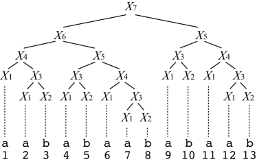
Figure 1: The derivation tree of SLP $\mathcal{T}=\{X_{1}\rightarrow\mathtt{a}$, $X_{2}\rightarrow\mathtt{b}$, $X_{3}\rightarrow X_{1}X_{2}$, $X_{4}\rightarrow X_{1}X_{3}$, $X_{5}\rightarrow X_{3}X_{4}$, $X_{6}\rightarrow X_{4}X_{5}$, $X_{7}\rightarrow X_{6}X_{5}\}$, representing string $T=\mathit{val}(X_{7})=\mathtt{aababaababaab}$.

A straight line program (SLP) is a set of assignments $\mathcal{T}=\{X_{1}\rightarrow expr_{1},X_{2}\rightarrow expr_{2},\ldots,X_{n}\rightarrow expr_{n}\}$, where each $X_{i}$ is a variable and each $expr_{i}$ is an expression, where $expr_{i}=a$ ($a\in\Sigma$), or $expr_{i}=X_{\ell(i)}X_{r(i)}$ ($i>\ell(i),r(i)$). It is essentially a context free grammar in the Chomsky normal form, that derives a single string. Let $\mathit{val}(X_{i})$ represent the string derived from variable $X_{i}$. To ease notation, we sometimes associate $\mathit{val}(X_{i})$ with $X_{i}$ and denote $|\mathit{val}(X_{i})|$ as $|X_{i}|$, and $\mathit{val}(X_{i})([u:v])$ as $X_{i}([u:v])$ for any interval $[u:v]$. An SLP $\mathcal{T}$ represents the string $T=\mathit{val}(X_{n})$. The size of the program $\mathcal{T}$ is the number $n$ of assignments in $\mathcal{T}$. Note that $|T|$ can be as large as $\Theta(2^{n})$. However, we assume as in various previous work on SLP, that the computer word size is at least $\log|T|$, and hence, values representing lengths and positions of $T$ in our algorithms can be manipulated in constant time.

The derivation tree of SLP $\mathcal{T}$ is a labeled ordered binary tree where each internal node is labeled with a non-terminal variable in $\{X_{1},\ldots,X_{n}\}$, and each leaf is labeled with a terminal character in $\Sigma$. The root node has label $X_{n}$. Let $\mathcal{V}$ denote the set of internal nodes in the derivation tree. For any internal node $v\in\mathcal{V}$, let $\langle v\rangle$ denote the index of its label $X_{\langle v\rangle}$. Node $v$ has a single child which is a leaf labeled with $c$ when $(X_{\langle v\rangle}\rightarrow c)\in\mathcal{T}$ for some $c\in\Sigma$, or $v$ has a left-child and right-child respectively denoted $\ell(v)$ and $r(v)$, when $(X_{\langle v\rangle}\rightarrow X_{\langle\ell(v)\rangle}X_{\langle r(v)\rangle})\in\mathcal{T}$. Each node $v$ of the tree derives $\mathit{val}(X_{\langle v\rangle})$, a substring of $T$, whose corresponding interval $\mathit{itv}(v)$, with $T(\mathit{itv}(v))=\mathit{val}(X_{\langle v\rangle})$, can be defined recursively as follows. If $v$ is the root node, then $\mathit{itv}(v)=[1:|T|]$. Otherwise, if $(X_{\langle v\rangle}\rightarrow X_{\langle\ell(v)\rangle}X_{\langle r(v)\rangle})\in\mathcal{T}$, then, $\mathit{itv}(\ell(v))=[b_{v}:b_{v}+|X_{\langle\ell(v)\rangle}|-1]$ and $\mathit{itv}(r(v))=[b_{v}+|X_{\langle\ell(v)\rangle}|:e_{v}]$, where $[b_{v}:e_{v}]=\mathit{itv}(v)$. Let $\mathit{vOcc}(X_{i})$ denote the number of times a variable $X_{i}$ occurs in the derivation tree, i.e., $\mathit{vOcc}(X_{i})=|\{v\mid X_{\langle v\rangle}=X_{i}\}|$. We assume that any variable $X_{i}$ is used at least once, that is $\mathit{vOcc}(X_{i})>0$.

For any interval $[b:e]$ of $T(1\leq b\leq e\leq|T|)$, let $\xi_{\mathcal{T}}(b,e)$ denote the deepest node $v$ in the derivation tree, which derives an interval containing $[b:e]$, that is, $\mathit{itv}(v)\supseteq[b:e]$, and no proper descendant of $v$ satisfies this condition. We say that node $v$ stabs interval $[b:e]$, and $X_{\langle v\rangle}$ is called the variable that stabs the interval. If $b=e$, we have that $(X_{\langle v\rangle}\rightarrow c)\in\mathcal{T}$ for some $c\in\Sigma$, and $\mathit{itv}(v)=b=e$. If $b<e$, then we have $(X_{\langle v\rangle}\rightarrow X_{\langle\ell(v)\rangle}X_{\langle r(v)\rangle})\in\mathcal{T}$, $b\in\mathit{itv}(\ell(v))$, and $e\in\mathit{itv}(r(v))$. When it is not confusing, we will sometimes use $\xi_{\mathcal{T}}(b,e)$ to denote the variable $X_{\langle\xi_{\mathcal{T}}(b,e)\rangle}$.

SLPs can be efficiently pre-processed to hold various information. $|X_{i}|$ and $\mathit{vOcc}(X_{i})$ can be computed for all variables $X_{i}(1\leq i\leq n)$ in a total of $O(n)$ time by a simple dynamic programming algorithm. Also, the following Lemma is useful for partial decompression of a prefix of a variable.

Lemma 1 ([8])

Given an SLP $\mathcal{T}=\{X_{i}\rightarrow\mathit{expr}_{i}\}_{i=1}^{n}$, it is possible to pre-process $\mathcal{T}$ in $O(n)$ time and space, so that for any variable $X_{i}$ and $1\leq j\leq|X_{i}|$, ${X_{i}}([1:j])$ can be computed in $O(j)$ time.

The formal statement of the problem we solve is:

Problem 1 ($q$-gram frequencies on SLP)

Given integer $q\geq 1$ and an SLP $\mathcal{T}$ of size $n$ that represents string $T$, output $(i,|\mathit{Occ}(T,P)|)$ for all $P\in\Sigma^{q}$ where $\mathit{Occ}(T,P)\neq\emptyset$, and some $i\in\mathit{Occ}(T,P)$.

Since the problem is very simple for $q=1$, we shall only consider the case for $q\geq 2$ for the rest of the paper. Note that although the number of distinct $q$-grams in $T$ is bounded by $O(qn)$, we would require an extra multiplicative $O(q)$ factor for the output if we output each $q$-gram explicitly as a string. In our algorithms to follow, we compute a compact, $O(qn)$-size representation of the output, from which each $q$-gram can be easily obtained in $O(q)$ time.

3 $O(qn)$ Algorithm [9]

In this section, we briefly describe the $O(qn)$ algorithm presented in [9]. The idea is to count occurrences of $q$-grams with respect to the variable that stabs its occurrence. The algorithm reduces Problem 1 to calculating the frequencies of all $q$-grams in a weighted set of strings, whose total length is $O(qn)$. Lemma 2 shows the key idea of the algorithm.

Lemma 2

For any SLP $\mathcal{T}=\{X_{i}\rightarrow\mathit{expr}_{i}\}_{i=1}^{n}$ that represents string $T$, integer $q\geq 2$, and $P\in\Sigma^{q}$, $|\mathit{Occ}(T,P)|=\sum_{i=1}^{n}\mathit{vOcc}(X_{i})\cdot|\mathit{Occ}(t_{i},P)|$, where $t_{i}=\mathit{suf}(\mathit{val}(X_{\ell(i)}),q-1)\mathit{pre}(\mathit{val}(X_{r(i)}),q-1)$.

Proof

For any $q\geq 2$, $v$ stabs the interval $[u:u+q-1]$ if and only if $[u:u+q-1]\subseteq[s_{v}:f_{v}]=\mathit{suf}(\mathit{itv}(\ell(v)),q-1)\cup\mathit{pre}(\mathit{itv}(r(v)),q-1)$. (See Fig. 2.) Also, since an occurrence of $X_{i}$ in the derivation tree always derives the same string $\mathit{val}(X_{i})$, $t_{i}=T([s_{v}:f_{v}])$ for any node $v$ such that $X_{\langle v\rangle}=X_{i}$. Therefore,

$$|\mathit{Occ}(T,P)|=\big{|}\{u>0\mid T([u:u+q-1])=P\}\big{|}$$

$$= \sum_{v\in\mathcal{V}}\big{|}\{u>0\mid\xi_{\mathcal{T}}(u,u+q-1)=v,j=u-s_{v}+1,X_{\langle v\rangle}([j:j+q-1])=P\}\big{|}$$

$$= \sum_{i=1}^{n}\sum_{v\in\mathcal{V}:X_{\langle v\rangle}=X_{i}}\big{|}\{u>0\mid\xi_{\mathcal{T}}(u,u+q-1)=v,j=u-s_{v}+1,X_{\langle v\rangle}([j:j+q-1])=P\}\big{|}$$

$$= \sum_{i=1}^{n}\sum_{v\in\mathcal{V}:X_{\langle v\rangle}=X_{i}}\mathit{Occ}(T([s_{v}:f_{v}]),P)=\sum_{i=1}^{n}\mathit{vOcc}(X_{i})\cdot\mathit{Occ}(t_{i},P).$$

∎

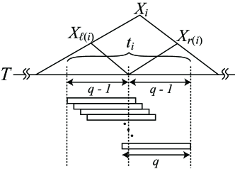
Figure 2: Length-$q$ intervals where $X_{\langle\xi_{\mathcal{T}}(u,u+q-1)\rangle}=X_{i}$, and $(X_{i}\rightarrow X_{\ell(i)}X_{r(i)})\in\mathcal{T}$.

From Lemma 2, we have that occurrence frequencies in $T$ are equivalent to occurrence frequencies in $t_{i}$ weighted by $\mathit{vOcc}(X_{i})$. Therefore, the $q$-gram frequencies problem can be regarded as obtaining the weighted frequencies of all $q$-grams in the set of strings $\{t_{1},\ldots,t_{n}\}$, where each occurrence of a $q$-gram in $t_{i}$ is weighted by $\mathit{vOcc}(X_{i})$. This can be further reduced to a weighted $q$-gram frequency problem for a single string $z$, where each position of $z$ holds a weight associated with the $q$-gram that starts at that position. String $z$ is constructed by concatenating all $t_{i}$’s with length at least $q$. The weights of positions corresponding to the first $|t_{i}|-(q-1)$ characters of $t_{i}$ will be $\mathit{vOcc}(X_{i})$, while the last $(q-1)$ positions will be $0$ so that superfluous $q$-grams generated by the concatenation are not counted. The remaining is a simple linear time algorithm using suffix and lcp arrays on the weighted string, thus solving the problem in $O(qn)$ time and space.

4 New Algorithm

We now describe our new algorithm which solves the $q$-gram frequencies problem on SLPs. The new algorithm basically follows the previous $O(qn)$ algorithm, but is an elegant refinement. The reduction for the previous $O(qn)$ algorithm leads to a fairly large amount of redundantly decompressed regions of the text as $q$ increases. This is due to the fact that the $t_{i}$’s are considered independently for each variable $X_{i}$, while neighboring $q$-grams that are stabbed by different variables actually share $q-1$ characters. The key idea of our new algorithm is to exploit this redundancy. (See Fig. 3.) In what follows, we introduce the concept of $q$-gram neighbors, and reduce the $q$-gram frequencies problem on SLP to a weighted $q$-gram frequencies problem on a weighted tree.

4.1 $q$-gram Neighbor Graph

We say that $X_{j}$ is a right $q$-gram neighbor of $X_{i}$ $(i\neq j)$, or equivalently, $X_{i}$ is a left $q$-gram neighbor of $X_{j}$, if for some integer $u\in[1:|T|-q]$, $X_{\langle\xi_{\mathcal{T}}(u,u+q-1)\rangle}=X_{i}$ and $X_{\langle\xi_{\mathcal{T}}(u+1,u+q)\rangle}=X_{j}$. Notice that $|X_{i}|$ and $|X_{j}|$ are both at least $q$ if $X_{i}$ and $X_{j}$ are right or left $q$-gram neighbors of each other.

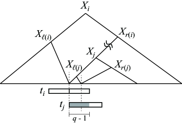
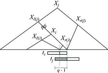
Figure 3: $q$-gram neighbors and redundancies. (Left) $X_{j}$ is a right $q$-gram neighbor of $X_{i}$, and $X_{i}$ is a left $q$-gram neighbor of $X_{j}$. Note that the right $q$-gram neighbor of $X_{i}$ is uniquely determined since $|X_{r(i)}|\geq q$ and it must be a descendant on the left most path rooted at $X_{r(i)}$, However, $X_{j}$ may have other left $q$-gram neighbors, since $|X_{\ell(j)}|<q$, and they must be ancestors of $X_{j}$. $t_{i}$ (resp. $t_{j}$) represents the string corresponding to the union of intervals $[u:u+q-1]$ where $X_{\langle\xi_{\mathcal{T}}(u,u+q-1)\rangle}=X_{i}$ (resp. $X_{\langle\xi_{\mathcal{T}}(u,u+q-1)\rangle}=X_{j}$). The shaded region depicts the string which is redundantly decompressed, if both $t_{i}$ and $t_{j}$ are considered independently. (Right) Shows the reverse case, when $|X_{r(i)}|<q$.

Definition 1

For $q\geq 2$, the right $q$-gram neighbor graph of SLP $\mathcal{T}=\{X_{i}\rightarrow expr_{i}\}_{i=1}^{n}$ is the directed graph $G_{q}=(V,E_{r})$, where

$$V = \{X_{i}\mid i\in\{1,\ldots,n\},|X_{i}|\geq q\}$$

$$E_{r} = \{(X_{i},X_{j})\mid X_{j}\mbox{ is a right $q$-gram neighbor of $X_{i}$ }\}$$

Note that there can be multiple right $q$-gram neighbors for a given variable. However, the total number of edges in the neighbor graph is bounded by $2n$, as will be shown below.

Lemma 3

Let $X_{j}$ be a right $q$-gram neighbor of $X_{i}$. If, $|X_{r(i)}|\geq q$, then $X_{j}$ is the label of the deepest variable on the left-most path of the derivation tree rooted at a node labeled $X_{r(i)}$ whose length is at least $q$. Otherwise, if $|X_{r(i)}|<q$, then $X_{i}$ is the label of the deepest variable on the right-most path rooted at a node labeled $X_{\ell(j)}$ whose length is at least $q$.

Proof

Suppose $|X_{r(i)}|\geq q$. Let $u$ be a position, where $X_{\langle\xi_{\mathcal{T}}(u,u+q-1)\rangle}=X_{i}$ and $X_{\langle\xi_{\mathcal{T}}(u+1,u+q)\rangle}=X_{j}$. Then, since the interval $[u+1:u+q]$ is a prefix of $\mathit{itv}(X_{r(i)})$, $X_{j}$ must be on the left most path rooted at $X_{r(i)}$. Since $X_{j}=X_{\langle\xi_{\mathcal{T}}(u+1,u+q)\rangle}$, the lemma follows from the definition of $\xi_{\mathcal{T}}$. The case for $|X_{r(i)}|<q$ is symmetrical and can be shown similarly. ∎

Lemma 4

For an arbitrary SLP $\mathcal{T}=\{X_{i}\rightarrow expr_{i}\}_{i=1}^{n}$ and integer $q\geq 2$, the number of edges in the right $q$-gram neighbor graph $G_{q}$ of $\mathcal{T}$ is at most $2n$.

Proof

Suppose $X_{j}$ is a right $q$-gram neighbor of $X_{i}$. From Lemma 3, we have that if $|X_{r(i)}|\geq q$, the right $q$-gram neighbor of $X_{i}$ is uniquely determined and that $|X_{\ell(j)}|<q$. Similarly, if $|X_{r(i)}|<q$, $|X_{\ell(j)}|\geq q$ and the left $q$-gram neighbor of $X_{j}$ is uniquely $X_{i}$. Therefore,

$$\sum_{i=1}^{n}|\{(X_{i},X_{j})\in E_{r}\mid|X_{r(i)}|\geq q\}|+\sum_{i=1}^{n}|\{(X_{i},X_{j})\in E_{r}\mid|X_{r(i)}|<q\}|$$

$$= \sum_{i=1}^{n}|\{(X_{i},X_{j})\in E_{r}\mid|X_{r(i)}|\geq q\}|+\sum_{i=1}^{n}|\{(X_{i},X_{j})\in E_{r}\mid|X_{\ell(j)}|\geq q\}|\leq 2n.$$

∎

Lemma 5

For an arbitrary SLP $\mathcal{T}=\{X_{i}\rightarrow expr_{i}\}_{i=1}^{n}$ and integer $q\geq 2$, the right $q$-gram neighbor graph $G_{q}$ of $\mathcal{T}$ can be constructed in $O(n)$ time.

Proof

For any variable $X_{i}$, let $\mathit{lm}_{q}(X_{i})$ and $\mathit{rm}_{q}(X_{i})$ respectively represent the index of the label of the deepest node with length at least $q$ on the left-most and right-most path in the derivation tree rooted at $X_{i}$, or $\mathit{null}$ if $|X_{i}|<q$. These values can be computed for all variables in a total of $O(n)$ time based on the following recursion: If $(X_{i}\rightarrow a)\in\mathcal{T}$ for some $a\in\Sigma$, then $\mathit{lm}_{q}(X_{i})=\mathit{rm}_{q}(X_{i})=\mathit{null}$. For $(X_{i}\rightarrow X_{\ell(i)}X_{r(i)})\in\mathcal{T}$,

$$\mathit{lm}_{q}(X_{i})=\begin{cases}\mathit{null}&\mbox{if }|X_{i}|<q,\\ i&\mbox{if }|X_{i}|\geq q\mbox{ and }|X_{\ell(i)}|<q,\\ \mathit{lm}_{q}(X_{\ell(i)})&\mbox{otherwise. }\end{cases}$$

$\mathit{rm}_{q}(X_{i})$ can be computed similarly. Finally,

$$E_{r} = \{(X_{i},X_{\mathit{lm}_{q}(X_{r(i)})})\mid\mathit{lm}_{q}(X_{r(i)})\neq\mathit{null},i=1,\ldots,n\}$$

$$\cup\{(X_{\mathit{rm}_{q}(X_{\ell(i)})},X_{i})\mid\mathit{rm}_{q}(X_{\ell(i)})\neq\mathit{null},i=1,\ldots,n\}.$$

∎

Lemma 6

Let $G_{q}=(V,E_{r})$ be the right $q$-gram neighbor graph of SLP $\mathcal{T}=\{X_{i}=expr_{i}\}_{i=1}^{n}$ representing string $T$, and let $X_{i_{1}}=X_{\langle\xi_{\mathcal{T}}(1,q)\rangle}$. Any variable $X_{j}\in V(i_{1}\neq j)$ is reachable from $X_{i_{1}}$, that is, there exists a directed path from $X_{i_{1}}$ to $X_{j}$ in $G_{q}$.

Proof

Straightforward, since any $q$-gram of $T$ except for the left most $T([1:q])$ has a $q$-gram on its left.∎

4.2 Weighted $q$-gram Frequencies Over a Trie

From Lemma 6, we have that the right $q$-gram neighbor graph is connected. Consider an arbitrary directed spanning tree rooted at $X_{i_{1}}=X_{\langle\xi_{\mathcal{T}}(1,q)\rangle}$ which can be obtained in linear time by a depth first traversal on $G_{q}$ from $X_{i_{1}}$. We define the label $\mathit{label}(X_{i})$ of each node $X_{i}$ of the $q$-gram neighbor graph, by

$$\mathit{label}(X_{i})=t_{i}[q:|t_{i}|]$$

where $t_{i}=\mathit{suf}(\mathit{val}(X_{\ell(i)}),q-1)\mathit{pre}(\mathit{val}(X_{r(i)}),q-1)$ as before. For convenience, let $X_{i_{0}}$ be a dummy variable such that $\mathit{label}(X_{i_{0}})=T([1:q-1])$, and $X_{r(i_{0})}=X_{i_{1}}$ (and so $(X_{i_{0}},X_{i_{1}})\in E_{r}$).

Lemma 7

Fix a directed spanning tree on the right $q$-gram neighbor graph of SLP $\mathcal{T}$, rooted at $X_{i_{0}}$. Consider a directed path $X_{i_{0}},\ldots,X_{i_{m}}$ on the spanning tree. The weighted $q$-gram frequencies on the string obtained by the concatenation $\mathit{label}(X_{i_{0}})\mathit{label}(X_{i_{1}})\cdots\mathit{label}(X_{i_{m}})$, where each occurrence of a $q$-gram that ends in a position in $\mathit{label}(X_{i_{j}})$ is weighted by $\mathit{vOcc}(X_{i_{j}})$, is equivalent to the weighted $q$-gram frequencies of strings $\{t_{i_{1}},\ldots t_{i_{m}}\}$ where each $q$-gram in $t_{i_{j}}$ is weighted by $\mathit{vOcc}(X_{i_{j}})$.

Proof

Proof by induction: for $m=1$, we have that $\mathit{label}(X_{i_{0}})\mathit{label}(X_{i_{1}})=t_{i_{1}}$. All $q$-grams in $t_{i_{1}}$ end in $t_{i_{1}}$ and so are weighted by $\mathit{vOcc}(X_{i_{1}})$. When $\mathit{label}(X_{i_{j}})$ is added to $\mathit{label}(X_{i_{0}})\cdots\mathit{label}(X_{i_{j-1}})$, $|\mathit{label}(X_{i_{j}})|$ new $q$-grams are formed, which correspond to $q$-grams in $t_{i_{j}}$, i.e. $|t_{i_{j}}|=q-1+|\mathit{label}(X_{i_{j}})|$, and $t_{i_{j}}$ is a suffix of $\mathit{label}(X_{i_{j-1}})\mathit{label}(X_{i_{j}})$. All the new $q$-grams end in $\mathit{label}(X_{i_{j}})$ and are thus weighted by $\mathit{vOcc}(X_{i_{j}})$. ∎

From Lemma 7, we can construct a weighted trie $\Upsilon$ based on a directed spanning tree of $G_{q}$ and $\mathit{label}()$, where the weighted $q$-grams in $\Upsilon$ (represented as length-$q$ paths) correspond to the occurrence frequencies of $q$-grams in $T$.

1 Construct right $q$-gram neighbor graph $G=(V,E_{r})$;

2 Calculate $\mathit{vOcc}(X_{i})$ for $i=1,\ldots,n$;

3 Calculate $|\mathit{label}(X_{i})|$ for $i=1,\ldots,n$;

4 for $i=0,\ldots,n$ do $\mathsf{visited}[i]=\mathsf{false}$;

5 $X_{i_{1}}=X_{\langle\xi_{\mathcal{T}}(1,q)\rangle}=\mathit{lm}_{q}(X_{n})$;

6 Define $X_{i_{0}}$ so that $X_{r(i_{0})}=X_{i_{1}}$ and $|\mathit{label}(X_{i_{0}})|=q-1$;

$\mathit{root}\leftarrow$ new node;

 // root of resulting trie

7 4.2($i_{0}$, $\mathit{root}$);

return $\mathit{root}$

Algorithm 1 Constructing weighted trie from SLP

[t]    BuildDepthFirst($i$, $\mathit{trieNode}$) // add prefix of $r(i)$ to trieNode while right neighbors of $i$ are unique $l\leftarrow 0$; $k\leftarrow i$;

2 while true do

3       $l\leftarrow l+|\mathit{label}(X_{k})|$;

4       $\mathsf{visited}[k]\leftarrow\mathsf{true}$;

5       // exit loop if right neighbor is possibly non-unique or is visited if $|X_{r(k)}|<q$ or $\mathsf{visited}[\mathit{lm}_{q}(X_{r(k)})]=\mathsf{true}$ then break;

6       $k\leftarrow\mathit{lm}_{q}(X_{r(k)})$;

7      

8 add new branch from $\mathit{trieNode}$ with string $X_{r(i)}([1:l])$;

9 let end of new branch be $\mathit{newTrieNode}$;

10 // If $|X_{r(k)}|<q$, there may be multiple right neighbors. // If $|X_{r(k)}|\geq q$, nothing is done because it has already been visited. for $X_{c}\in\{X_{j}\mid(X_{k},X_{j})\in E_{r}\}$ do

11       if $\mathsf{visited}[c]=\mathsf{false}$ then

12             4.2 ($X_{c}$, $\mathit{newTrieNode}$);

13            

14      

 

Lemma 8

$\Upsilon$ can be constructed in time linear in its size.

Proof

See Algorithm 1. Let $G$ be the $q$-gram neighbor graph. We construct $\Upsilon$ in a depth first manner starting at $X_{i_{0}}$. The crux of the algorithm is that rather than computing $\mathit{label}()$ separately for each variable, we are able to aggregate the $\mathit{label}()$s and limit all partial decompressions of variables to prefixes of variables, so that Lemma 1 can be used.

Any directed acyclic path on $G$ starting at $X_{i_{0}}$ can be segmented into multiple sequences of variables, where each sequence $X_{i_{j}},\ldots,X_{i_{k}}$ is such that $j$ is the only integer in $[j:k]$ such that $j=0$ or $|X_{r(i_{j-1})}|<q$. From Lemma 3, we have that $X_{i_{j+1}},\ldots,X_{i_{k}}$ are uniquely determined. If $j>0$, $\mathit{label}(X_{i_{j}})$ is a prefix of $\mathit{val}(X_{r(i_{j})})$ since $|X_{r(i_{j-1})}|<q$ (see Fig. 3 Right), and if $j=0$, $\mathit{label}(X_{i_{0}})$ is again a prefix of $\mathit{val}(X_{r(i_{0})})=\mathit{val}(X_{i_{1}})$. It is not difficult to see that $\mathit{label}(X_{i_{j}})\cdots\mathit{label}(X_{i_{k}})$ is also a prefix of $X_{r(i_{j})}$ since $X_{i_{j+1}},\ldots,X_{i_{k}}$ are all descendants of $X_{r(i_{j})}$, and each $\mathit{label}()$ extends the partially decompressed string to consider consecutive $q$-grams in $X_{r(i_{j})}$. Since prefixes of variables of SLPs can be decompressed in time proportional to the output size with linear time pre-processing (Lemma 1), the lemma follows. ∎

We only illustrate how the character labels are determined in the pseudo-code of Algorithm 1. It is straightforward to assign a weight $\mathit{vOcc}(X_{k})$ to each node of $\Upsilon$ that corresponds to $\mathit{label}(X_{k})$.

Lemma 9

The number of edges in $\Upsilon$ is $(q-1)+\sum\{|t_{i}|-(q-1)\mid|X_{i}|\geq q,i=1,\ldots,n\}=|T|-\mathit{dup}(q,\mathcal{T})$ where

$$\mathit{dup}(q,\mathcal{T})=\sum\{(\mathit{vOcc}(X_{i})-1)\cdot(|t_{i}|-(q-1))\mid|X_{i}|\geq q,i=1,\ldots,n\}\}$$

Proof

$(q-1)+\sum\{|t_{i}|-(q-1)\mid|X_{i}|\geq q,i=1,\ldots,n\}$ is straight forward from the definition of $\mathit{label}(X_{i})$ and the construction of $\Upsilon$. Concerning $\mathit{dup}$, each variable $X_{i}$ occurs $\mathit{vOcc}(X_{i})$ times in the derivation tree, but only once in the directed spanning tree. This means that for each occurrence after the first, the size of $\Upsilon$ is reduced by $|\mathit{label}(X_{i})|=|t_{i}|-(q-1)$ compared to $T$. Therefore, the lemma follows. ∎

To efficiently count the weighted $q$-gram frequencies on $\Upsilon$, we can use suffix trees. A suffix tree for a trie is defined as a generalized suffix tree for the set of strings represented in the trie as leaf to root paths. The following is known.

Lemma 10 ([18])

Given a trie of size $m$, the suffix tree for the trie can be constructed in $O(m)$ time and space.

With a suffix tree, it is a simple exercise to solve the weighted $q$-gram frequencies problem on $\Upsilon$ in linear time. In fact, it is known that the suffix array for the common suffix trie can also be constructed in linear time [6], as well as its longest common prefix array [13], which can also be used to solve the problem in linear time.

Corollary 1

The weighted $q$-gram frequencies problem on a trie of size $m$ can be solved in $O(m)$ time and space.

From the above arguments, the theorem follows.

Theorem 4.1

The $q$-gram frequencies problem on an SLP $\mathcal{T}$ of size $n$, representing string $T$ can be solved in $O(\min\{qn,|T|-\mathit{dup}(q,\mathcal{T})\})$ time and space.

Note that since each $q\leq|t_{i}|\leq 2(q-1)$, and $|\mathit{label}(X_{i})|=|t_{i}|-(q-1)$, the total length of decompressions made by the algorithm, i.e. the size of the reduced problem, is at least halved and can be as small as $1/q$ (when all $|t_{i}|=q$, for example, in an SLP that represents LZ78 compression), compared to the previous $O(qn)$ algorithm.

5 Preliminary Experiments

We first evaluate the size of the trie $\Upsilon$ induced from the right $q$-gram neighbor graph, on which the running time of the new algorithm of Section 4 is dependent. We used data sets obtained from Pizza & Chili Corpus, and constructed SLPs using the RE-PAIR [14] compression algorithm. Each data is of size 200MB. Table 1 shows the sizes of $\Upsilon$ for different values of $q$, in comparison with the total length of strings $t_{i}$, on which the previous $O(qn)$-time algorithm of Section 3 works. We cumulated the lengths of all $t_{i}$’s only for those satisfying $|t_{i}|\geq q$, since no $q$-gram can occur in $t_{i}$’s with $|t_{i}|<q$. Observe that for all values of $q$ and for all data sets, the size of $\Upsilon$ (i.e., the total number of characters in $\Upsilon$) is smaller than those of $t_{i}$’s and the original string.

Table 1: A comparison of the size of $\Upsilon$ and the total length of strings $t_{i}$ for SLPs that represent textual data from Pizza & Chili Corpus. The length of the original text is 209,715,200. The SLPs were constructed by RE-PAIR [14].

	XML			DNA			ENGLISH			PROTEINS
$q$	$\sum|t_{i}|$	size of $\Upsilon$		$\sum|t_{i}|$	size of $\Upsilon$		$\sum|t_{i}|$	size of $\Upsilon$		$\sum|t_{i}|$	size of $\Upsilon$
2	19,082,988	9,541,495		46,342,894	23,171,448		37,889,802	18,944,902		64,751,926	32,375,964
3	37,966,315	18,889,991		92,684,656	46,341,894		75,611,002	37,728,884		129,449,835	64,698,833
4	55,983,397	27,443,734		139,011,475	69,497,812		112,835,471	56,066,348		191,045,216	93,940,205
5	72,878,965	35,108,101		185,200,662	92,516,690		148,938,576	73,434,080		243,692,809	114,655,697
6	88,786,480	42,095,985		230,769,162	114,916,322		183,493,406	89,491,371		280,408,504	123,786,699
7	103,862,589	48,533,013		274,845,524	135,829,862		215,975,218	103,840,108		301,810,933	127,510,939
8	118,214,023	54,500,142		315,811,932	153,659,844		246,127,485	116,339,295		311,863,817	129,618,754
9	131,868,777	60,045,009		352,780,338	167,598,570		273,622,444	126,884,532		318,432,611	131,240,299
10	144,946,389	65,201,880		385,636,192	177,808,192		298,303,942	135,549,310		325,028,658	132,658,662
15	204,193,702	86,915,492		477,568,585	196,448,347		379,441,314	157,558,436		347,993,213	138,182,717
20	255,371,699	104,476,074		497,607,690	200,561,823		409,295,884	162,738,812		364,230,234	142,213,239
50	424,505,759	157,069,100		530,329,749	206,796,322		429,380,290	165,882,006		416,966,397	156,257,977
100	537,677,786	192,816,929		536,349,226	207,838,417		435,843,895	167,313,028		463,766,667	168,544,608

The construction of the suffix tree or array for a trie, as well as the algorithm for Lemma 1, require various tools such as level ancestor queries [5, 2, 1] for which we did not have an efficient implementation. Therefore, we try to assess the practical impact of the reduced problem size using a simplified version of our new algorithm. We compared three algorithms (NSA, SSA, STSA) that count the occurrence frequencies of all $q$-grams in a text given as an SLP. NSA is the $O(|T|)$-time algorithm which works on the uncompressed text, using suffix and LCP arrays. SSA is our previous $O(qn)$-time algorithm [9], and STSA is a simplified version of our new algorithm. STSA further reduces the weighted $q$-gram frequencies problem on $\Upsilon$, to a weighted $q$-gram frequencies problem on a single string as follows: instead of constructing $\Upsilon$, each branch of $\Upsilon$ (on line 4.2 of 4.2) is appended into a single string. The $q$-grams that are represented in the branching edges of $\Upsilon$ can be represented in the single string, by redundantly adding $\mathit{suf}(X_{r(i)}([1:l]),q-1)$ in front of the string corresponding to the next branch. This leads to some duplicate partial decompression, but the resulting string is still always shorter than the string produced by our previous algorithm [9]. The partial decompression of $X_{r(i)}([1:l])$ is implemented using a simple $O(h+l)$ algorithm, where $h$ is the height of the SLP which can be as large as $O(n)$.

All computations were conducted on a Mac Pro (Mid 2010) with MacOS X Lion 10.7.2, and 2 x 2.93GHz 6-Core Xeon processors and 64GB Memory, only utilizing a single process/thread at once. The program was compiled using the GNU C++ compiler (g++) 4.6.2 with the -Ofast option for optimization. The running times were measured in seconds, after reading the uncompressed text into memory for NSA, and after reading the SLP that represents the text into memory for SSA and STSA. Each computation was repeated at least 3 times, and the average was taken.

Table 2 summarizes the running times of the three algorithms. SSA and STSA computed weighted $q$-gram frequencies on $t_{i}$ and $\Upsilon$, respectively. Since the difference between the total length of $t_{i}$ and the size of $\Upsilon$ becomes larger as $q$ increases, STSA outperforms SSA when the value of $q$ is not small. In fact, in Table 2 SSA2 was faster than SSA for all values of $q>3$. STSA was even faster than NSA on the XML data whenever $q\leq 20$. What is interesting is that STSA outperformed NSA on the ENGLISH data when $q=100$.

Table 2: Running time in seconds for SLPs that represent textual data from Pizza & Chili Corpus. The SLPs were constructed by RE-PAIR [14]. Bold numbers represent the fastest time for each data and $q$. STSA is faster than SSA whenever $q>3$.

	XML				DNA				ENGLISH				PROTEINS
$q$	NSA	SSA	STSA		NSA	SSA	STSA		NSA	SSA	STSA		NSA	SSA	STSA
2	41.67	6.53	7.63		61.28	19.27	22.73		56.77	16.31	19.23		60.16	27.13	30.71
3	41.46	10.96	10.92		61.28	29.14	31.07		56.77	25.58	25.57		60.53	47.53	50.65
4	41.87	16.27	14.5		61.65	42.22	41.69		56.77	37.48	34.95		60.86	74.89	73.51
5	41.85	21.33	17.42		61.57	56.26	54.21		57.09	49.83	45.21		60.53	101.64	79.1
6	41.9	25.77	20.07		60.91	73.11	68.63		57.11	62.91	55.28		61.18	123.74	75.83
7	41.73	30.14	21.94		60.89	90.88	82.85		56.64	75.69	63.35		61.14	136.12	72.62
8	41.92	34.22	23.97		61.57	110.3	93.46		57.27	87.9	69.7		61.39	142.29	71.08
9	41.92	37.9	25.08		61.26	127.29	96.07		57.09	100.24	73.63		61.36	148.12	69.88
10	41.76	41.28	26.45		60.94	143.31	96.26		57.43	110.85	75.68		61.42	149.73	69.34
15	41.95	58.21	32.21		61.72	190.88	84.86		57.31	146.89	70.63		60.42	160.58	66.57
20	41.82	74.61	39.62		61.36	203.03	83.13		57.65	161.12	64.8		61.01	165.03	66.09
50	42.07	134.38	53.98		61.73	216.6	78.0		57.02	166.67	57.89		61.05	181.14	66.36
100	41.81	181.23	60.18		61.46	217.05	75.91		57.3	166.67	56.86		60.69	197.33	69.9

References

- [1] Bender, M.A., Farach-Colton, M.: The level ancestor problem simplified. Theor. Comput. Sci. 321(1), 5–12 (2004)
- [2] Berkman, O., Vishkin, U.: Finding level-ancestors in trees. J. Comput. System Sci. 48(2), 214–230 (1994)
- [3] Claude, F., Navarro, G.: Self-indexed grammar-based compression. Fundamenta Informaticae (to appear)
- [4] Crochemore, M., Landau, G.M., Ziv-Ukelson, M.: A subquadratic sequence alignment algorithm for unrestricted scoring matrices. SIAM J. Comput. 32(6), 1654–1673 (2003)
- [5] Dietz, P.: Finding level-ancestors in dynamic trees. In: Proc. WADS. pp. 32–40 (1991)
- [6] Ferragina, P., Luccio, F., Manzini, G., Muthukrishnan, S.: Compressing and indexing labeled trees, with applications. J. ACM 57(1) (2009)
- [7] Gawrychowski, P.: Pattern matching in Lempel-Ziv compressed strings: Fast, simple, and deterministic. In: Proc. ESA 2011. pp. 421–432 (2011)
- [8] Ga̧sieniec, L., Kolpakov, R., Potapov, I., Sant, P.: Real-time traversal in grammar-based compressed files. In: Proc. DCC’05. p. 458 (2005)
- [9] Goto, K., Bannai, H., Inenaga, S., Takeda, M.: Fast -gram mining on SLP compressed strings. In: Proc. SPIRE’11. pp. 289–289 (2011)
- [10] Hermelin, D., Landau, G.M., Landau, S., Weimann, O.: A unified algorithm for accelerating edit-distance computation via text-compression. In: Proc. STACS’09. pp. 529–540 (2009)
- [11] Inenaga, S., Bannai, H.: Finding characteristic substring from compressed texts. In: Proc. The Prague Stringology Conference 2009. pp. 40–54 (2009), full version to appear in the International Journal of Foundations of Computer Science
- [12] Karpinski, M., Rytter, W., Shinohara, A.: An efficient pattern-matching algorithm for strings with short descriptions. Nordic Journal of Computing 4, 172–186 (1997)
- [13] Kimura, D., Kashima, H.: A linear time subpath kernel for trees. In: IEICE Technical Report. vol. IBISML2011-85, pp. 291–298 (2011)
- [14] Larsson, N.J., Moffat, A.: Offline dictionary-based compression. In: Proc. DCC’99. pp. 296–305. IEEE Computer Society (1999)
- [15] Nevill-Manning, C.G., Witten, I.H., Maulsby, D.L.: Compression by induction of hierarchical grammars. In: Proc. DCC’94. pp. 244–253 (1994)
- [16] Rytter, W.: Application of Lempel-Ziv factorization to the approximation of grammar-based compression. Theor. Comput. Sci. 302(1–3), 211–222 (2003)
- [17] Shibata, Y., Kida, T., Fukamachi, S., Takeda, M., Shinohara, A., Shinohara, T., Arikawa, S.: Speeding up pattern matching by text compression. In: Proc. CIAC. pp. 306–315 (2000)
- [18] Shibuya, T.: Constructing the suffix tree of a tree with a large alphabet. IEICE Transactions on Fundamentals of Electronics, Communications and Computer Sciences E86-A(5), 1061–1066 (2003)
- [19] Storer, J., Szymanski, T.: Data compression via textual substitution. Journal of the ACM 29(4), 928–951 (1982)
- [20] Welch, T.A.: A technique for high performance data compression. IEEE Computer 17, 8–19 (1984)
- [21] Ziv, J., Lempel, A.: A universal algorithm for sequential data compression. IEEE Transactions on Information Theory IT-23(3), 337–349 (1977)
- [22] Ziv, J., Lempel, A.: Compression of individual sequences via variable-length coding. IEEE Transactions on Information Theory 24(5), 530–536 (1978)