On Perturbations of Almost Distance-Regular Graphs

Abstract

In this paper we show that certain almost distance-regular graphs, the so-called $h$-punctually walk-regular graphs, can be characterized through the cospectrality of their perturbed graphs. A graph $G$ with diameter $D$ is called $h$-punctually walk-regular, for a given $h\leq D$, if the number of paths of length $\ell$ between a pair of vertices $u,v$ at distance $h$ depends only on $\ell$. The graph perturbations considered here are deleting a vertex, adding a loop, adding a pendant edge, adding/removing an edge, amalgamating vertices, and adding a bridging vertex. We show that for walk-regular graphs some of these operations are equivalent, in the sense that one perturbation produces cospectral graphs if and only if the others do. Our study is based on the theory of graph perturbations developed by Cvetković, Godsil, McKay, Rowlinson, Schwenk, and others. As a consequence, some new characterizations of distance-regular graphs are obtained.

Keywords: Distance-regular graph, Walk-regular graph, Eigenvalues, Perturbation, Cospectral graphs

2010 Mathematics Subject Classification: 05C50, 05E30

1 Introduction

Both the theory of distance-regular graphs and that of graph perturbations have been widely developed in the last decades. The importance of the former can be grasped from the comment in the preface of the comprehensive monograph of Brouwer, Cohen, and Neumaier [1]: “Most finite objects bearing ‘enough regularity’ are closely related to certain distance-regular graphs.” Thus, many characterizations of a combinatorial and algebraic nature of distance-regular graphs are known (see [13]), and they have given rise to several generalizations, such as association schemes (see Brouwer and Haemers [2]) and almost distance-regular graphs [7]. With respect to the latter, the spectral properties of modified (or ‘perturbed’) graphs have relevance in Chemistry, in the construction of isospectral molecules, as well as in other areas of graph theory (as in the reconstruction conjecture); see Cvetković, Doob, and Sachs [4], Rowlinson [22, 23], and Schwenk [26]. The aim of this paper is to put together different ideas and results from both theories to show that certain almost distance-regular graphs, the so-called $h$-punctually walk-regular (or $h$-punctually spectrum-regular) graphs, can be characterized through the cospectrality of their perturbed graphs. We consider three one-vertex perturbations, namely, vertex deletion, adding a loop at a vertex, and adding a pendant edge at a vertex. These three perturbations are extended to pairs of vertices to obtain two-vertex ‘separate’ perturbations. We also consider three two-vertex ‘joint’ perturbations, namely adding/removing an edge, amalgamating two vertices, and adding a bridging vertex. We show that for walk-regular graphs all these two-vertex operations are equivalent, in the sense that one perturbation produces cospectral graphs if and only if the others do. We also consider perturbations on a set of vertices, and their impact on almost distance-regular graphs. As a consequence, we obtain some new characterizations of distance-regular graphs, in terms of the cospectrality of their perturbed graphs.

2 Preliminaries

In this section we give the basic definitions, notation and results on which our study is based. For completeness, we prove again some known results. Accordingly, we also recall some basic results on the computation of determinants which are used in our study.

2.1 Graphs and their spectra

Let $G=(V,E)$ be a (connected) graph with vertex set $V$ and edge set $E$. The adjacency between vertices $u,v\in V$, that is $uv\in E$, is denoted by $u\sim v$, and their distance is $\mathop{\partial}\nolimits(u,v)$. Let ${\mbox{\boldmath$A$}}=(a_{uv})$ be the adjacency matrix of $G$, with characteristic polynomial $\phi_{G}(x)$, and spectrum $\mathop{\rm sp}\nolimits G=\{\lambda_{0}^{m_{0}},\lambda_{1}^{m_{1}},\dots,\lambda_{d}^{m_{d}}\}$, where the different eigenvalues of $G$ are in decreasing order, $\lambda_{0}>\lambda_{1}>\cdots>\lambda_{d}$, and the superscripts stand for their multiplicities $m_{i}=m(\lambda_{i})$. For $i=0,1,\ldots,d$, let ${\mbox{\boldmath$E$}}_{i}$ be the principal idempotent of $A$, which corresponds to the orthogonal projection onto the eigenspace ${\cal E}_{i}=\mathop{\rm Ker}\nolimits(\lambda_{i}{\mbox{\boldmath$I$}}-{\mbox{\boldmath$A$}})$. In particular, if $G$ is regular, ${\mbox{\boldmath$E$}}_{0}=\frac{1}{n}{\mbox{\boldmath$J$}}$, where $J$ stands for the all-$1$ matrix. As is well known, the idempotents satisfy the following properties: ${\mbox{\boldmath$E$}}_{i}{\mbox{\boldmath$E$}}_{j}=\delta_{ij}{\mbox{\boldmath$E$}}_{i}$ (with $\delta_{ij}$ being the Kronecker delta), ${\mbox{\boldmath$A$}}{\mbox{\boldmath$E$}}_{i}=\lambda_{i}{\mbox{\boldmath$E$}}_{i}$, and $q({\mbox{\boldmath$A$}})=\sum_{i=0}^{d}q(\lambda_{i}){\mbox{\boldmath$E$}}_{i}$ for every rational function $q$ that is well-defined at each eigenvalue of $A$; see, for instance, Godsil [16]. The $uv$-entry $m_{uv}(\lambda_{i})=({\mbox{\boldmath$E$}}_{i})_{uv}$ of the idempotent ${\mbox{\boldmath$E$}}_{i}$ is called the crossed $(uv$-$)$local multiplicity of $\lambda_{i}$. As some direct consequences of the above properties, the following lemma gives some properties of these parameters (see, for example, [12]).

Lemma 2.1

For $u,v\in V$, the crossed local multiplicities of each eigenvalue $\lambda_{i}$, $i=0,1,\ldots,d$, satisfy the following properties:

• $\sum_{i=0}^{d}m_{uv}(\lambda_{i})=\delta_{uv}$.

• $\sum_{w\sim v}m_{uw}(\lambda_{i})=\lambda_{i}m_{uv}(\lambda_{i})$.

• $a_{uv}^{(\ell)}=({\mbox{\boldmath$A$}}^{\ell})_{uv}=\sum_{i=0}^{d}m_{uv}(\lambda_{i})\lambda_{i}^{\ell}$.

Note that the $uv$-entry $a_{uv}^{(\ell)}$ of the power matrix ${\mbox{\boldmath$A$}}^{\ell}$ is equal to the number of walks of length $\ell$ between vertices $u,v$. Rowlinson [24] showed that a graph $G$ is distance-regular if and only if this number of walks only depends on $\ell=0,1,\ldots,d$ and the distance $\mathop{\partial}\nolimits(u,v)$ between $u$ and $v$. Similarly, $G$ is distance-regular if and only if its local crossed multiplicities $m_{uv}(\lambda_{i})$ only depend on $\lambda_{i}$ and $\mathop{\partial}\nolimits(u,v)$; see [13]. Inspired by these characterizations, the authors [7] introduced the following concepts as different approaches to ‘almost distance-regularity’. We say that a graph $G$ with diameter $D$ and $d+1$ distinct eigenvalues is $h$-punctually walk-regular, for a given $h\leq D$, if for every $\ell\geq 0$ the number of walks of length $\ell$ between a pair of vertices $u,v$ at distance $\mathop{\partial}\nolimits(u,v)=h$ does not depend on $u,v$. Similarly, we say that $G$ is $h$-punctually spectrum-regular, for a given $h\leq D$ if for all $i\leq d$, the crossed $uv$-local multiplicities of $\lambda_{i}$ are the same for all pairs of vertices $u,v$ at distance $\mathop{\partial}\nolimits(u,v)=h$. In this case, we write $m_{uv}(\lambda_{i})=m_{hi}$. The concepts of $h$-punctual walk-regularity and $h$-punctual spectrum-regularity are equivalent. For $h=0$, the concepts are equivalent to walk-regularity (a concept introduced by Godsil and McKay in [17]) and spectrum-regularity (see Fiol and Garriga [14]), respectively.

2.2 Graph perturbations

As mentioned above, we consider three basic graph perturbations which involve a given vertex $u\in V$:

• $G-u$ is the graph obtained from $G$ by removing $u$ and all the edges incident to it.

• $G+uu$ is the (pseudo)graph obtained from $G$ by adding a loop at $u$. (In this case the graph obtained has adjacency matrix as expected, with its $uu$-entry equal to $1$.)

• $G+u\bar{u}$ is the graph obtained from $G$ by adding a pendant edge at $u$ (thus creating a new vertex $\bar{u}$).

Two vertices $u,v$ satisfying $\mathop{\rm sp}\nolimits(G-u)=\mathop{\rm sp}\nolimits(G-v)$ were called cospectral by Herndon and Ellzey [19]. We say that a graph is $0$-punctually cospectral when all its vertices are cospectral; a concept that we will generalize below. It is well-known that a graph is $0$-punctually cospectral if and only if it is walk-regular; see Proposition 3.1, where we also relate this to the perturbations P2 and P3. In fact, the proof of Proposition 3.1 implies that cospectral vertices $u,v$ can be equivalently defined by requiring that $\mathop{\rm sp}\nolimits(G+uu)=\mathop{\rm sp}\nolimits(G+vv)$ or $\mathop{\rm sp}\nolimits(G+u\bar{u})=\mathop{\rm sp}\nolimits(G+v\bar{v})$.

Given a vertex subset $U\subset V$, we can also consider the graphs obtained by applying any of the above perturbations to every vertex of $U$, with natural notation $G-U$, $G+UU$ and $G+U\bar{U}$. In particular, when $U=\{u,v\}$, we also write $G-u-v$, $G+uu+vv$ and $G+u\bar{u}+v\bar{v}$.

Building on the concept of cospectral vertices, Schwenk [26] considered the analogue for sets: Two vertex subsets $U,U^{\prime}\subset V$ are removal-cospectral if there exists a one-to-one mapping $U\rightarrow U^{\prime}$ such that, for every $W\subset U$, the graphs $G-W$ and $G-W^{\prime}$ are cospectral. A main result of his paper was the following necessary condition for two sets being removal-cospectral:

Theorem 2.2

[26] If $U,U^{\prime}$ are removal-cospectral sets, then $a_{uv}^{(\ell)}=a_{u^{\prime}v^{\prime}}^{(\ell)}$ for all pairs of vertices $u,v\in U$ and all $\ell\geq 0$.

Godsil [15] proved that two vertex subsets $U,U^{\prime}$ are removal-cospectral if and only if for every subset $W\subset U$ with at most two vertices, the subsets $W,W^{\prime}$ are removal-cospectral (for both an alternative proof and a geometric interpretation of this result, see Rowlinson [23]).

As a consequence of Theorem 2.2, notice that for $\{u,v\}$ and $\{u^{\prime},v^{\prime}\}$ to be removal-cospectral we need that $\mathop{\partial}\nolimits(u,v)=\mathop{\partial}\nolimits(u^{\prime},v^{\prime})$. Otherwise, if $r=\mathop{\partial}\nolimits(u,v)<\mathop{\partial}\nolimits(u^{\prime},v^{\prime})$, say, we would have $a_{uv}^{(r)}>0$ whereas $a_{u^{\prime}v^{\prime}}^{(r)}=0$. Inspired by this property, we say that two vertex subsets are isometric when there exists a one-to-one mapping $U\rightarrow U^{\prime}$ such that, for every pair $u,v\in U$, we have $\mathop{\partial}\nolimits(u,v)=\mathop{\partial}\nolimits(u^{\prime},v^{\prime})$. So, if two sets are removal-cospectral then they are also isometric. In the last section, we will show that the converse is also true for distance-regular graphs.

For example, in the Petersen graph all cocliques (that is, independent sets) of size $3$ are removal-cospectral. Since there are two different kinds of such cocliques (one of these is indicated in Figure 1 by the empty dots, and the other by the thick dots), removing them gives a pair of cospectral but non-isomorphic graphs. This is the left pair in Figure 2. The right pair is obtained by adding edges to the cocliques. This also gives cospectral but non-isomorphic graphs since, as was proved by Schwenk [26], if $U$ and $U^{\prime}$ are removal-cospectral sets, then any graph may be attached to all the points of $U$ and to the points of $U^{\prime}$ with the two graphs so formed being cospectral.

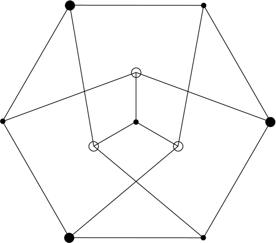
Figure 1: Petersen graph with 3-cocliques

Figure 2: Two pairs of cospectral graphs: removing vertices and adding edges

In our framework of almost distance-regular graphs, the case when the two vertices of $W$ are at a given distance proves to be specially relevant, and leads us to the following definition: A graph $G$ with diameter $D$ is $h$-punctually cospectral, for a given $h\leq D$, when, for all pairs of vertices $u,v$ and $w,z$, both at distance $\mathop{\partial}\nolimits(u,v)=\mathop{\partial}\nolimits(w,z)=h$, we have $\mathop{\rm sp}\nolimits(G-u-v)=\mathop{\rm sp}\nolimits(G-w-z)$. Again, we will show later (in Lemma 4.1) that this concept can also be defined by using the other graph perturbations considered here. Notice that, since there are no restrictions on either pair of vertices, except for their distance, this is equivalent to the sets $W=\{u,v\}$ and $W^{\prime}=\{u^{\prime},v^{\prime}\}$, with both mappings $u^{\prime}=w$, $v^{\prime}=z$ and $u^{\prime}=z$, $v^{\prime}=w$, being removal-cospectral.

Then, using our terminology, Schwenk’s theorem implies the following corollary:

Corollary 2.3

If a graph $G$ is $j$-punctually cospectral for $j=0,h$, then it is $j$-punctually walk-regular for $j=0,h$.

Answering a question of Schwenk [26], Rowlinson [23] proved the following characterization of removal-cospectral sets, which we give in terms of the local crossed multiplicities:

Theorem 2.4

[23] The vertex (non-empty) subsets $U,U^{\prime}$ are removal-cospectral if and only if $m_{uv}(\lambda_{i})=m_{u^{\prime}v^{\prime}}(\lambda_{i})$ for all $u,v\in U$ and $i=0,1,\ldots,d$.

In fact, Rowlinson gave his result in terms of the so-called star sequences $\{{\mbox{\boldmath$E$}}_{i}{\mbox{\boldmath$e$}}_{u}:u\in U\}$, $i=0,1,\ldots,d$ and $\{{\mbox{\boldmath$E$}}_{i}{\mbox{\boldmath$e$}}_{u^{\prime}}:u^{\prime}\in U^{\prime}\}$, $i=0,1,\ldots,d$, where ${\mbox{\boldmath$e$}}_{u}$ stands for the $u$-th unit vector.

Again, in our context we have the following consequence:

Corollary 2.5

A graph $G$ is $j$-punctually cospectral for $j=0,h$ if and only if it is $j$-punctually spectrum-regular for $j=0,h$.

We remind the reader that the concepts of $h$-punctually walk-regularity and $h$-punctually spectrum-regularity are equivalent, so Corollary 2.5 implies Corollary 2.3. As this corollary is one of the crucial characterizations for us, we will restate (and prove) it later on as Theorem 4.2.

2.3 Computing determinants

Our first study will use the two following lemmas to compute determinants. A proof of the first result can be found, for instance, in Godsil [16, p. 19]. For the argument for Jacobi’s determinant identity, see Rowlinson [23, p. 212], for example.

Lemma 2.6

Let $A$ and $B$ be two $n\times n$ matrices. Then, $\det({\mbox{\boldmath$A$}}+{\mbox{\boldmath$B$}})$ equals the sum of the determinants of the $2^{n}$ matrices obtained by replacing every subset of the columns of $A$ by the corresponding subset of the columns of $B$.

In particular, for all column vectors $x$, $y$ of size $n$ and $n\times(n-1)$ matrix $M$, we have the well-known linearity property

$$\det({\mbox{\boldmath$x$}}+{\mbox{\boldmath$y$}}|\mbox{\boldmath$M$})=\det({\mbox{\boldmath$x$}}|\mbox{\boldmath$M$})+\det({\mbox{\boldmath$y$}}|\mbox{\boldmath$M$}).$$ (1)

Lemma 2.7

$($Jacobi’s determinant identity$)$ Let $A$ be an invertible matrix with rows and columns indexed by the elements of $V$. For a given nontrivial subset $U$ of $V$, let ${\mbox{\boldmath$A$}}[U]$ denote the principal submatrix of $A$ on $U$. Let $\overline{U}=V\setminus U$. Then,

$$\det{\mbox{\boldmath$A$}}[U]=\det{\mbox{\boldmath$A$}}\det{\mbox{\boldmath$A$}}^{-1}[\overline{U}].$$

3 Walk-regular graphs

Our main results were inspired by the following characterizations of walk-regular graphs:

Proposition 3.1

The following statements are equivalent:

• $G$ is walk-regular

• $G$ is spectrum-regular.

• $\mathop{\rm sp}\nolimits(G-u)=\mathop{\rm sp}\nolimits(G-v)$ for all vertices $u,v$.

• $\mathop{\rm sp}\nolimits(G+uu)=\mathop{\rm sp}\nolimits(G+vv)$ for all vertices $u,v$.

• $\mathop{\rm sp}\nolimits(G+u\bar{u})=\mathop{\rm sp}\nolimits(G+v\bar{v})$ for all vertices $u,v$.

$Proof.$   Let $G$ have adjacency matrix $A$. The equivalence $(a)\iff(b)$ was proved by Delorme and Tillich [11] and Fiol and Garriga [14].

Godsil and McKay [18] obtained a relation between a walk-generating function of $G$ and the characteristic polynomials of $G$ and $G-u$. This can be formulated (see also [6, p. 83]) as

$$\phi_{G-u}(x)=\phi_{G}(x)\sum_{i=0}^{d}\frac{m_{u}(\lambda_{i})}{x-\lambda_{i}}.$$

This can also be proved by using Lemma 2.7. Indeed, let $U=V\setminus\{u\}$ and ${\mbox{\boldmath$C$}}=x{\mbox{\boldmath$I$}}-{\mbox{\boldmath$A$}}$. Then, as ${\mbox{\boldmath$C$}}^{-1}=\sum_{i=0}^{d}\frac{{\mbox{\boldmath$E$}}_{i}}{x-\lambda_{i}}$, we have

$$\phi_{G-u}(x)=\det{\mbox{\boldmath$C$}}[U]=\det{\mbox{\boldmath$C$}}\det{\mbox{\boldmath$C$}}^{-1}[\{u\}]=\phi_{G}(x)\sum_{i=0}^{d}\frac{{\mbox{\boldmath$E$}}_{i}[\{u\}]}{x-\lambda_{i}}=\phi_{G}(x)\sum_{i=0}^{d}\frac{m_{u}(\lambda_{i})}{x-\lambda_{i}}.$$

Therefore $(b)\Rightarrow(c)$. Conversely, if $\phi_{G-u}(x)=\phi_{G-v}(x)$, then the limit

$$\lim_{x\rightarrow\lambda_{i}}\frac{\phi_{G-u}(x)}{\phi_{G-v}(x)}=\frac{m_{u}(\lambda_{i})}{m_{v}(\lambda_{i})}$$

yields that $m_{u}(\lambda_{i})=m_{v}(\lambda_{i})$ for every $i=0,1,\ldots,d$, hence $(c)\Rightarrow(b)$.

If we apply Lemma 2.6 to compute the determinant of $(x{\mbox{\boldmath$I$}}-{\mbox{\boldmath$A$}})+(-{\mbox{\boldmath$B$}})$, where $B$ is the matrix with the only non-zero entry $({\mbox{\boldmath$B$}})_{uu}=1$, we get

$$\phi_{G+uu}(x)=\phi_{G}(x)-\phi_{G-u}(x),$$ (2)

thus proving the equivalence $(c)\iff(d)$.

Finally, the natural determinantal expansion of

$$x{\mbox{\boldmath$I$}}-{\mbox{\boldmath$A$}}_{\bar{u}}=\left(\begin{array}[]{cc}x&\mbox{$-1$\ \ \ \ }\mbox{\bf 0}^{\top}\\ \begin{array}[]{c}-1\\ \mbox{\bf 0}\end{array}&x{\mbox{\boldmath$I$}}-{\mbox{\boldmath$A$}}\end{array}\right),$$

where ${\mbox{\boldmath$A$}}_{\bar{u}}$ is the adjacency matrix of $G+u\bar{u}$ (with the first two rows and columns indexed by the vertices $\bar{u}$ and $u$), gives the well-known result

$$\phi_{G+u\bar{u}}(x)=x\phi_{G}(x)-\phi_{G-u}(x)$$ (3)

(see also, for instance, Rowlinson [22]), thus proving that $(c)\iff(e)$.  $\Box$

Thus, we have just proved that a graph $G$ is ($0$-punctually) walk-regular or ($0$-punctually) spectrum-regular if and only it is $0$-punctually cospectral, a concept which, as was claimed, can be defined through any of the considered graph perturbations. In the next section, we generalize this result.

4 $h$-Punctually walk-regular graphs

To obtain some characterizations and properties of $h$-punctually walk-regular graphs, we consider some basic graph perturbations involving two vertices. With this aim, we first perturb the vertices ‘separately’, as done in the previous section. Second, similar characterizations are derived when we perturb the vertices ‘together’.

4.1 Separate perturbations

Let us first prove the following lemma concerning perturbations P1-P3 for pairs of vertices in walk-regular graphs:

Lemma 4.1

For all pairs of vertices $u,v$ and $w,z$ of a walk-regular graph $G$, the following statements are equivalent:

• $\mathop{\rm sp}\nolimits(G-u-v)=\mathop{\rm sp}\nolimits(G-w-z)$.

• $\mathop{\rm sp}\nolimits(G+uu+vv)=\mathop{\rm sp}\nolimits(G+ww+zz)$.

• $\mathop{\rm sp}\nolimits(G+u\bar{u}+v\bar{v})=\mathop{\rm sp}\nolimits(G+w\bar{w}+z\bar{z})$.

$Proof.$   The equivalence $(a)\iff(b)$ follows by applying repeatedly Eq. (2) to obtain

$$\phi_{G-u-v}(x)-\phi_{G+uu+vv}(x)=\phi_{G-u}(x)-\phi_{G+vv}(x),$$

and using Proposition 3.1. Analogously, from Eq. (3) we get

$$\phi_{G-u-v}(x)-\phi_{G+u\bar{u}+v\bar{v}}(x)=x\phi_{G-u}(x)-x\phi_{G+v\bar{v}}(x),$$

which proves $(a)\iff(c)$.  $\Box$

Notice that, by this result and Proposition 3.1, each of the above conditions ($a$)-($c$) is equivalent to the sets $\{u,v\}$ and $\{w,z\}$ being removal-cospectral. Moreover, as mentioned before, this allows us to define $h$-punctually cospectrality by requiring that every pair of vertices at distance $h$ satisfies one of these conditions.

In turn, this leads to the following characterization of $h$-punctually walk-regular graphs. It is, in a sense, a restatement of Corollary 2.5.

Theorem 4.2

For a walk-regular graph $G$ with diameter $D$ and a given integer $h\leq D$, the following statements are equivalent:

• $G$ is $h$-punctually walk-regular.

• $G$ is $h$-punctually spectrum-regular.

• $G$ is $h$-punctually cospectral.

$Proof.$   The equivalence $(a)\iff(b)$ was proved by the authors in [7]. To prove the equivalence $(b)\iff(c)$, we use Lemma 2.7, and follow the same line of reasoning as Rowlinson [23]. Indeed, let $U=V\setminus\{u,v\}$ with $\mathop{\partial}\nolimits(u,v)=h$, and ${\mbox{\boldmath$C$}}=x{\mbox{\boldmath$I$}}-{\mbox{\boldmath$A$}}$. Then,

$$\phi_{G-u-v}(x) = \det{\mbox{\boldmath$C$}}[U]=\det{\mbox{\boldmath$C$}}\det{\mbox{\boldmath$C$}}^{-1}[\{u,v\}]$$ (6)

$$= \phi_{G}(x)\det\left(\sum_{i=0}^{d}\frac{{\mbox{\boldmath$E$}}_{i}[\{u,v\}]}{x-\lambda_{i}}\right)$$

$$= \phi_{G}(x)\det\left(\sum_{i=0}^{d}\frac{1}{x-\lambda_{i}}\left(\begin{array}[]{cc}m_{uu}(\lambda_{i})&m_{uv}(\lambda_{i})\\ m_{uv}(\lambda_{i})&m_{vv}(\lambda_{i})\end{array}\right)\right)$$

$$= \phi_{G}(x)\left[\left(\sum_{i=0}^{d}\frac{m_{0i}}{x-\lambda_{i}}\right)^{2}-\left(\sum_{i=0}^{d}\frac{m_{uv}(\lambda_{i})}{x-\lambda_{i}}\right)^{2}\right],$$ (7)

where we have used that, as $G$ is walk-regular, $m_{uu}(\lambda_{i})=m_{vv}(\lambda_{i})=m_{0i}$. Then, if $G$ is $h$-punctually spectrum-regular, $m_{uv}(\lambda_{i})=m_{hi}$ and, hence, $\phi_{G-u-v}(x)$ does not depend on $u,v$. This proves $(b)\Rightarrow(c)$. Conversely, if $\phi_{G-u-v}(x)=\phi_{G-w-z}(x)$ for some vertices $w,z$ at distance $\mathop{\partial}\nolimits(w,z)=h$, Eq. (7) yields

$$\left(\sum_{i=0}^{d}\frac{m_{uv}(\lambda_{i})}{x-\lambda_{i}}\right)^{2}=\left(\sum_{i=0}^{d}\frac{m_{wz}(\lambda_{i})}{x-\lambda_{i}}\right)^{2}$$

for all $x\neq\lambda_{0},\lambda_{1},\ldots,\lambda_{d}$. Therefore,

$$\sum_{i=0}^{d}\frac{m_{uv}(\lambda_{i})}{x-\lambda_{i}}=\pm\sum_{i=0}^{d}\frac{m_{wz}(\lambda_{i})}{x-\lambda_{i}}$$

(since, as $p^{2}=q^{2}\Rightarrow p=\pm q$ holds for polynomials, it also holds for rational functions). Consequently, taking limits $x\rightarrow\lambda_{i}$, we have that either $m_{wz}(\lambda_{i})=m_{uv}(\lambda_{i})$ for $i=0,1,\ldots,d$, or $m_{wz}(\lambda_{i})=-m_{uv}(\lambda_{i})$ for $i=0,1,\ldots,d$. But, since $m_{uv}(\lambda_{0})=m_{wz}(\lambda_{0})=\frac{1}{n}$, we must rule out the second possibility and $G$ is $h$-punctually spectrum-regular, thus proving that $(c)\Rightarrow(b)$.  $\Box$

4.2 Joint perturbations

We now consider the following perturbations involving two given vertices $u,v$:

• $G\pm uv$ is the graph obtained from $G$ by flipping the (non-)edge $uv$. (That is, changing the edge $uv$ into a non-edge or vice versa.)

• $G_{u+v}$ is the (pseudo)graph obtained from $G$ by amalgamating the vertices $u$ and $v$ (if $u\sim v$ then the edge $uv$ becomes a loop; if $u$ and $v$ have common neighbors, then multiple edges arise; the ‘new’ vertex is denoted by $u+v$).

• $G+u\bar{u}v$ is the graph obtained from $G$ by adding the 2-path $u\bar{u}v$ (thus creating a new so-called bridging vertex $\bar{u}$).

In the case that the graphs $G+u\bar{u}v$ and $G+w\bar{w}z$ are cospectral, the pairs $(u,v)$ and $(w,z)$ are called isospectral; see Lowe and Soto [20]. In the following result, we show that for walk-regular graphs, isospectral pairs can also be defined by requiring cospectrality of the graphs obtained from perturbations P4-P5.

Proposition 4.3

Let $u,v$ and $w,z$ be pairs of vertices of a walk-regular graph $G$ such that $u\sim v$ if and only if $w\sim z$. Then the following statements are equivalent:

• $\mathop{\rm sp}\nolimits(G\pm uv)=\mathop{\rm sp}\nolimits(G\pm wz)$.

• $\mathop{\rm sp}\nolimits G_{u+v}=\mathop{\rm sp}\nolimits G_{w+z}$.

• $\mathop{\rm sp}\nolimits(G+u\bar{u}v)=\mathop{\rm sp}\nolimits(G+w\bar{w}z)$.

$Proof.$   We will prove that each of the above conditions is equivalent to $m_{uv}(\lambda_{i})=m_{wz}(\lambda_{i})$, for all $i=0,1,\ldots,d$. With respect to $(a)$, note that, when $u\not\sim v$, the adjacency matrix of the graph $G+uv$ can be written as

$${\mbox{\boldmath$A$}}_{+uv}=\left(\begin{array}[]{ccc}0&1&{\mbox{\boldmath$y$}}^{\top}\\ 1&0&{\mbox{\boldmath$z$}}^{\top}\\ {\mbox{\boldmath$y$}}&{\mbox{\boldmath$z$}}&{\mbox{\boldmath$A$}}^{*}\end{array}\right)$$

where ${\mbox{\boldmath$A$}}^{*}$ is the adjacency matrix of $G-u-v$. Then, by applying twice Eq. (1) (to the first column and row) we have:

$$\det({\mbox{\boldmath$x$}}{\mbox{\boldmath$I$}}-{\mbox{\boldmath$A$}}_{+uv}) = \det\left(\begin{array}[]{ccc}x&0&-{\mbox{\boldmath$y$}}^{\top}\\ 0&x&-{\mbox{\boldmath$z$}}^{\top}\\ -{\mbox{\boldmath$y$}}&-{\mbox{\boldmath$z$}}&x{\mbox{\boldmath$I$}}-{\mbox{\boldmath$A$}}^{*}\end{array}\right)+\det\left(\begin{array}[]{ccc}0&-1&\mbox{\bf 0}^{\top}\\ 0&x&-{\mbox{\boldmath$z$}}^{\top}\\ -{\mbox{\boldmath$y$}}&-{\mbox{\boldmath$z$}}&x{\mbox{\boldmath$I$}}-{\mbox{\boldmath$A$}}^{*}\end{array}\right)$$

$$+ \det\left(\begin{array}[]{ccc}0&-1&\mbox{\bf 0}^{\top}\\ -1&x&-{\mbox{\boldmath$z$}}^{\top}\\ \mbox{\bf 0}&-{\mbox{\boldmath$z$}}&x{\mbox{\boldmath$I$}}-{\mbox{\boldmath$A$}}^{*}\end{array}\right)+\det\left(\begin{array}[]{ccc}0&0&-{\mbox{\boldmath$y$}}^{\top}\\ -1&x&-{\mbox{\boldmath$z$}}^{\top}\\ \mbox{\bf 0}&-{\mbox{\boldmath$z$}}&x{\mbox{\boldmath$I$}}-{\mbox{\boldmath$A$}}^{*}\end{array}\right).$$

Thus, with $\Psi_{uv}(x)$ denoting the $uv$-cofactor of $x{\mbox{\boldmath$I$}}-{\mbox{\boldmath$A$}}$ (where $A$ is the adjacency matrix of $G$), we get

$$\phi_{G+uv}(x)=\phi_{G}(x)-\phi_{G-u-v}(x)-2\Psi_{uv}(x).$$ (10)

This equation was also derived by Rowlinson [21]. Moreover, using a similar reasoning, Rowlinson [23] proved that, if $u\sim v$, we have

$$\phi_{G-uv}(x)=\phi_{G}(x)-\phi_{G-u-v}(x)+2\Psi_{uv}(x).$$

Then, from Eq. (7) and since the $uv$-cofactor $\Psi_{uv}(x)$ can be computed as:

$$\Psi_{uv}(x)=\det(x{\mbox{\boldmath$I$}}-{\mbox{\boldmath$A$}})((x{\mbox{\boldmath$I$}}-{\mbox{\boldmath$A$}})^{-1})_{uv}=\phi_{G}(x)\sum_{i=0}^{d}\frac{m_{uv}(\lambda_{i})}{x-\lambda_{i}},$$ (11)

we get

$$\phi_{G\pm uv}(x)=\phi_{G}(x)\left(1-\left(\sum_{i=0}^{d}\frac{m_{0i}}{x-\lambda_{i}}\right)^{2}+\left(\sum_{i=0}^{d}\frac{m_{uv}(\lambda_{i})}{x-\lambda_{i}}\right)^{2}\mp 2\sum_{i=0}^{d}\frac{m_{uv}(\lambda_{i})}{x-\lambda_{i}}\right).$$ (12)

Therefore $(a)$ is equivalent to

$$\left(\sum_{i=0}^{d}\frac{m_{uv}(\lambda_{i})}{x-\lambda_{i}}\mp 1\right)^{2}=\left(\sum_{i=0}^{d}\frac{m_{wz}(\lambda_{i})}{x-\lambda_{i}}\mp 1\right)^{2}.$$

By the same reasoning as in the proof of Theorem 4.2, this is equivalent to $m_{uv}(\lambda_{i})=m_{wz}(\lambda_{i})$ for $i=0,1,\ldots,d$.

For $(b)$ we use similar techniques. Indeed, we now apply the formula

$$\phi_{G_{u+v}}(x)=\phi_{G-u}(x)+\phi_{G-v}(x)-(x-a_{uv})\phi_{G-u-v}(x)-2\Psi_{uv}(x),$$ (13)

which is proved similarly as Eq. (10) (or by using $(2.8)$ and $(2.9)$ in Rowlinson [23] and Eq. (2)). Using Eqs. (7) and (11), it thus follows that $(b)$ is equivalent to

$$(x-a_{uv})\left(\sum_{i=0}^{d}\frac{m_{uv}(\lambda_{i})}{x-\lambda_{i}}\right)^{2}-2\sum_{i=0}^{d}\frac{m_{uv}(\lambda_{i})}{x-\lambda_{i}}=(x-a_{uv})\left(\sum_{i=0}^{d}\frac{m_{wz}(\lambda_{i})}{x-\lambda_{i}}\right)^{2}-2\sum_{i=0}^{d}\frac{m_{wz}(\lambda_{i})}{x-\lambda_{i}},$$

which, with $f(x)=\sum_{i=0}^{d}\frac{m_{uv}(\lambda_{i})}{x-\lambda_{i}}$ and $g(x)=\sum_{i=0}^{d}\frac{m_{wz}(\lambda_{i})}{x-\lambda_{i}}$, can be written as

$$([x-a_{uv}][f(x)+g(x)]-2)[f(x)-g(x)]=0.$$

The factor $[x-a_{uv}][f(x)+g(x)]-2$ in this equation cannot be zero. Indeed, this could only happen if say $\lambda_{j}=a_{uv}$ and $m_{uv}(\lambda_{i})+m_{wz}(\lambda_{i})$ would be 2 for $i=j$, and 0 otherwise. This however leads to a contradiction by Lemma 2.1(a). Hence, $(b)$ is equivalent to $f(x)-g(x)=0$, which leads again to $m_{uv}(\lambda_{i})=m_{wz}(\lambda_{i})$, $i=0,1,\ldots,d$.

Finally, case $(c)$ is managed by using the formula

$$\phi_{G+u\bar{u}v}(x)=\phi_{G}(x)\left(x-2\sum_{i=0}^{d}\frac{m_{0i}+m_{uv}(\lambda_{i})}{x-\lambda_{i}}\right),$$

(see Lowe and Soto [20] or Rowlinson [23, p. 216]).  $\Box$

It is perhaps good to remind the reader that the condition $m_{uv}(\lambda_{i})=m_{wz}(\lambda_{i})$ for all $i=0,1,\ldots,d$ implies that $u$ and $v$ are at the same distance as $w$ and $z$ (by Lemma 2.1$(c)$). Inspired by this and the above result, we say that a graph $G$ with diameter $D$ is $h$-punctually isospectral, for a given $h\leq D$, when every pair of vertices at distance $h$ satisfies one of the conditions in Proposition 4.3. As a corollary of its proof, we then obtain the following characterization of $h$-punctually walk-regular (or $h$-punctually spectrum-regular) graphs.

Corollary 4.4

For a walk-regular graph $G$ with diameter $D$ and a given integer $h\leq D$, the following statements are equivalent:

• $G$ is $h$-punctually walk-regular.

• $G$ is $h$-punctually spectrum-regular.

• $G$ is $h$-punctually isospectral.

We finish this section with an example of an almost distance-regular graph that can be used to produce many kinds of cospectral graphs by applying the above perturbations. The graph we use is one of the thirteen cubic graphs with integral spectrum. These graphs were classified by Bussemaker and Cvetković [3] and Schwenk [25]. Of these graphs we take the one that is cospectral (with spectrum $\{\pm 3^{1},\pm 2^{4},\pm 1^{5}\}$), but not isomorphic, with the Desargues graph; see Figure 3. This graph can be obtained by switching from the Desargues graph (take the four right-most vertices as switching set) and also by twisting it (in a similar way as in the twisted Grassmann graphs of [10]); cf. [9, Sect. 3.2]. It is a bipartite graph with diameter $D=5$ that is almost distance-regular in the sense that it is $h$-punctually walk-regular for all $h$ except $h=3$. It has two orbits of vertices under the action of its automorphism group; the middle twelve vertices are different from the others. This means that if we remove a vertex from the middle, and remove a vertex from the left four, we obtain non-isomorphic graphs that are cospectral (apply the above with $h=0$). These graphs are shown as the left pair in Figure 4. There are two kinds of edges, three kinds of pairs of vertices at distance 2, and two kinds of vertices at distance 4. These (for example) give cospectral graphs as shown on the right in Figure 4, and in Figures 5 and 6, respectively. There is only one kind of pair of vertices at distance 5, so these cannot be used to get non-isomorphic but cospectral graphs. We finally remark that this example can be generalized easily to other twisted graphs that are described in [9, Sect. 3.1-2]; for example the distance-regular twisted Grassmann graphs.

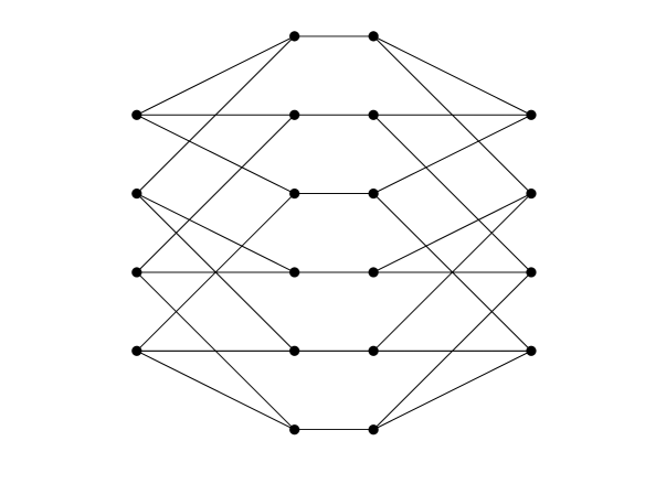
Figure 3: Bussemaker-Cvetković-Schwenk (twisted Desargues) graph

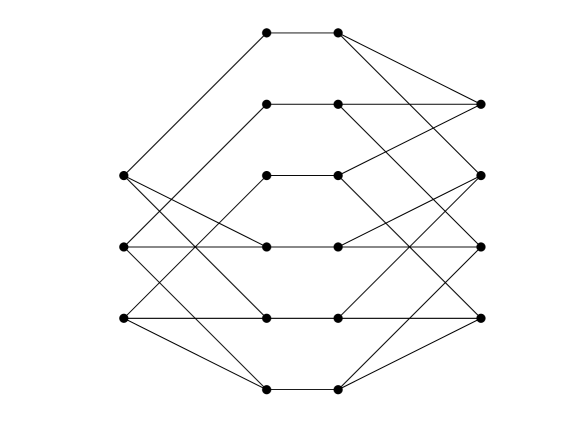
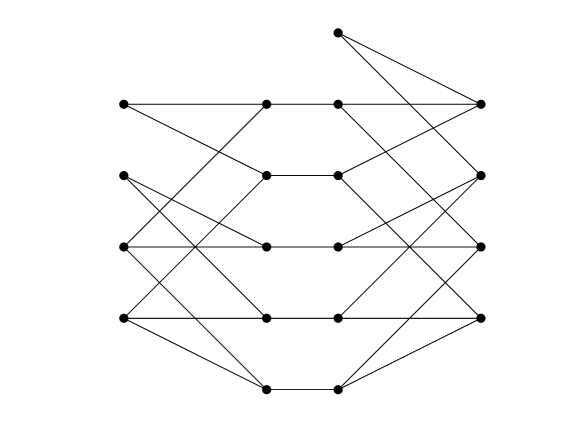
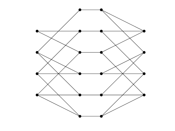
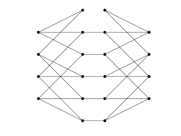
Figure 4: Pairs of cospectral graphs; removing vertices ($h=0$) and removing edges ($h=1$)

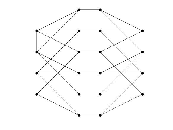
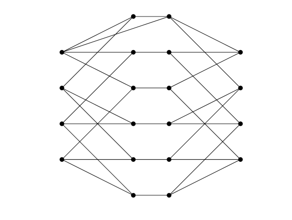
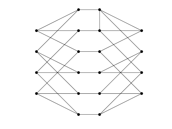
Figure 5: Triple of cospectral graphs; adding edges ($h=2$)

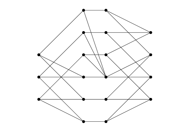
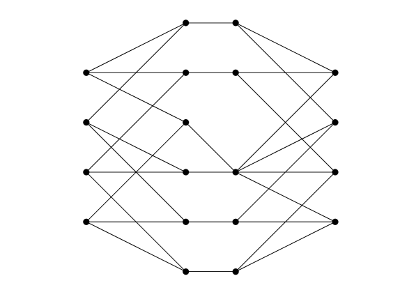
Figure 6: Pair of cospectral graphs; amalgamating vertices ($h=4$)

4.3 Multiple perturbations

For the sake of simplicity, we have only considered perturbations in a single graph $G$ so far. One could however also use the above perturbations in cospectral graphs $G$ and $G^{\prime}$ to get new cospectral graphs (as is well known from the literature). The conditions for this to work are similar as before: the crossed local multiplicities $m_{uv}(\lambda_{i})$ (in $G$) and $m^{\prime}_{wz}(\lambda_{i})$ (in $G^{\prime}$) should be the same for all $i=0,1,\ldots,d$ (or alternatively: the number of walks $a_{uv}^{(\ell)}$ (in $G$) and $a_{wz}^{\prime(\ell)}$ (in $G^{\prime}$) should be the same for all $\ell$).

Consider the Desargues graph, for example. This graph is cospectral to the above mentioned twisted Desargues graph. By removing a vertex ($h=0$), removing an edge ($h=1$), adding an edge $(h=2)$, and amalgamating vertices ($h=4)$ in the Desargues graph, one gets cospectral graphs of the graphs in the above figures. One could even exploit the case $h=5$ now.

For the next step — multiple perturbations — it is hard to avoid working with different (but cospectral) graphs. We next consider removal-cospectral sets $U,U^{\prime}$ belonging to cospectral (but not necessarily isomorphic) graphs $G,G^{\prime}$ (i.e., there exists a one-to-one mapping $U\rightarrow U^{\prime}$ such that, for every $W\subset U$, the graphs $G-W$ and $G^{\prime}-W^{\prime}$ are cospectral), as is usually done in the literature. The following proposition shows that all perturbations P1-P6 leave the property of two sets being removal-cospectral invariant, and gives new insight into some of the previous implications.

Proposition 4.5

Let $U$ and $U^{\prime}$ be removal-cospectral sets in cospectral graphs $G$ and $G^{\prime}$, and let $u,v\in U$ with corresponding vertices $u^{\prime},v^{\prime}\in U^{\prime}$. Let $\mathaccent 869{U},\mathaccent 869{U}^{\prime}$ be the sets obtained from $U,U^{\prime}$ after perturbing vertices $u$ and $u^{\prime}$ according to one of the perturbations P1-P3, or perturbing pairs of vertices $u,v$ and $u^{\prime},v^{\prime}$ through one of the perturbations P4-P6, where possible new vertices $u+v$, $\bar{u}$, $\bar{u}^{\prime}$ are included in $\mathaccent 869{U},\mathaccent 869{U}^{\prime}$. Let $\mathaccent 869{G}$ and $\mathaccent 869{G}^{\prime}$ be the resulting perturbed graphs. Then, the sets $\mathaccent 869{U},\mathaccent 869{U}^{\prime}$ are removal-cospectral in $\mathaccent 869{G}$ and $\mathaccent 869{G}^{\prime}$.

$Proof.$   We only prove the result for amalgamation (that is, P5), as the other cases are either very simple, or similar, or follow from Schwenk’s results in [26]. Thus, let us amalgamate $u,v\in U$ and $u^{\prime},v^{\prime}\in U^{\prime}$ to obtain $\mathaccent 869{G}=G_{u+v}$ and $\mathaccent 869{G}^{\prime}=G^{\prime}_{u^{\prime}+v^{\prime}}$. Now, consider a subset $S\subset\mathaccent 869{U}$ and its corresponding set $S^{\prime}\subset\mathaccent 869{U}^{\prime}$. We should prove that $G_{u+v}-S$ and $G^{\prime}_{u^{\prime}+v^{\prime}}-S$ are cospectral. To do this, we must consider two cases: If $u+v\in S$, then $G_{u+v}-S=G-(S\cup\{u,v\})$ and $G^{\prime}_{u^{\prime}+v^{\prime}}-S^{\prime}=G^{\prime}-(S^{\prime}\cup\{u^{\prime},v^{\prime}\})$. Hence, these two graphs are cospectral. Otherwise, if $u+v\not\in S$, then $G_{u+v}-S=(G-S)_{u+v}$ and $G^{\prime}_{u^{\prime}+v^{\prime}}-S^{\prime}=(G-S^{\prime})_{u^{\prime}+v^{\prime}}$, and these graphs are also cospectral because $U\setminus S$ and $U^{\prime}\setminus S^{\prime}$ are removal-cospectral in $G-S$ and $G^{\prime}-S^{\prime}$ (notice that, since $u,v\in U\setminus S$ and $u^{\prime},v^{\prime}\in U^{\prime}\setminus S^{\prime}$, we can apply Eq. (13) or repeat the above argument).  $\Box$

As a consequence, notice that the different one-vertex and two-vertex perturbations can be repeated over and over again to obtain different cospectral graphs $\mathaccent 869{G}$ and $\mathaccent 869{G}^{\prime}$. In other words, from two removal-cospectral sets $U,U^{\prime}$, one can, for example, amalgamate several vertices, or combine amalgamation with other operations such an edge removal/addition (hence also contract an edge), adding pendant edges, etc., to obtain new removal-cospectral sets $\mathaccent 869{U},\mathaccent 869{U}^{\prime}$ in the corresponding cospectral graphs $\mathaccent 869{G},\mathaccent 869{G}^{\prime}$. This suggests the following definition: Two vertex subsets $U,U^{\prime}$ of cospectral graphs $G,G^{\prime}$ are called perturb-cospectral if for all subsets $S\subset U$ and $S^{\prime}\subset U^{\prime}$, the perturbed graphs $\mathaccent 869{G}$ and $\mathaccent 869{G}^{\prime}$, obtained by applying P1-P6 to corresponding vertices of $U$ and $U^{\prime}$, are cospectral.

5 Distance-regular graphs

In this section we use the above results to obtain some new characterizations of distance-regular graphs.

In [7], the authors considered also the following concepts: A graph $G$ is $m$-walk-regular (respectively $m$-spectrum-regular) when it is $i$-punctually walk-regular (respectively $i$-punctually spectrum-regular) for every $i\leq m$. Similarly, we say that $G$ is $m$-cospectral (respectively, $m$-isospectral) when it is $i$-punctually cospectral (respectively, $i$-punctually isospectral) for every $i\leq m$. Using these definitions, Theorem 4.2 and Corollary 4.4 have the following direct consequence:

Corollary 5.1

For a walk-regular graph $G$ with diameter $D$ and a given integer $m\leq D$, the following statements are equivalent:

• $G$ is $m$-walk-regular.

• $G$ is $m$-spectrum-regular.

• $G$ is $m$-cospectral.

• $G$ is $m$-isospectral.

Moreover, as mentioned in Section 2.1, Rowlinson [24] proved that a graph $G$ is distance-regular if and only if it is $D$-walk-regular. Hence, we get the following characterization:

Theorem 5.2

Let $G$ be a graph with diameter $D$. Then, the following statements are equivalent:

• $G$ is distance-regular.

• $G$ is $D$-cospectral.

• $G$ is $D$-isospectral.

In fact, notice that we also proved the following result:

Theorem 5.3

A graph $G=(V,E)$ is distance-regular if and only if every two isometric subsets $U,U^{\prime}\subset V$ are perturb-cospectral.

Part of the case $D=2$ of Theorem 5.2 was already observed by Cvetković and Rowlinson [5]; they showed that if $G$ is strongly regular, then $\phi_{G-u-v}(x)$ depends only on whether or not $u$ and $v$ are adjacent. See also the observation by Godsil on cospectral graphs in strongly regular graphs in [8, Prop. 8].

Acknowledgement The authors are grateful to Ernest Garriga, Willem Haemers, and Peter Rowlinson for discussions on the topic of this paper. They also thank an anonymous referee for several useful comments. Research supported by the Ministerio de Educación y Ciencia, Spain, and the European Regional Development Fund under project MTM2008-06620-C03-01 and by the Catalan Research Council under project 2009SGR1387.

References

- [1] A.E. Brouwer, A.M. Cohen, and A. Neumaier, Distance-Regular Graphs, Springer-Verlag, Berlin-New York, 1989.
- [2] A.E. Brouwer and W.H. Haemers, Association schemes, in: Handbook of Combinatorics Vol. 1,2, 747–771, Elsevier, Amsterdam, 1995.
- [3] F.C. Bussemaker and D. Cvetković, There are exactly 13 connected, cubic, integral graphs, Univ. Beograd Publ. Elek. Fak., Ser. Mat. Fiz. 544-576 (1976), 43–48.
- [4] D. Cvetković, M. Doob, and H. Sachs, Spectra of Graphs, Academic Press, New York, 1980.
- [5] D. Cvetković and P. Rowlinson, Seeking counterexamples to the reconstruction conjecture: a research note, in: Proc. 8th Yugoslav Seminar on Graph Theory, Novi Sad, 1987 (ed. R. Tošić et al.) 52–62, Univ. Novi Sad, Inst. Math., 1989.
- [6] D. Cvetković, P. Rowlinson, and S. Simić, Eigenspaces of Graphs, Cambridge University Press, 1997.
- [7] C. Dalfó, E.R. van Dam, M.A. Fiol, E. Garriga, and B.L. Gorissen, On almost distance-regular graphs, J. Combin. Theory Ser. A 118 (2011), 1094–1113.
- [8] E.R. van Dam and W.H. Haemers, Developments on spectral characterizations of graphs, Discrete Math. 309 (2009), 576–586.
- [9] E.R. van Dam, W.H. Haemers, J.H. Koolen, and E. Spence, Characterizing distance-regularity of graphs by the spectrum, J. Combin. Theory Ser. A 113 (2006), 1805–1820.
- [10] E.R. van Dam and J.H. Koolen, A new family of distance-regular graphs with unbounded diameter, Inventiones Math. 162 (2005), 189–193.
- [11] C. Delorme and J.P. Tillich, Eigenvalues, eigenspaces and distances to subsets, Discrete Math. 165/166 (1997), 161–184.
- [12] M.A. Fiol, On pseudo-distance-regularity, Linear Algebra Appl. 323 (2001), 145–165.
- [13] M.A. Fiol, Algebraic characterizations of distance-regular graphs, Discrete Math. 246 (2002), 111–129.
- [14] M.A. Fiol and E. Garriga, The alternating and adjacency polynomials, and their relation with the spectra and diameters of graphs, Discrete Appl. Math. 87 (1998), 77–97.
- [15] C.D. Godsil, Walk generating functions, Christoffel-Darboux identities and the adjacency matrix of a graph, Combin. Probab. Comput. 1 (1992), no. 1, 13–25.
- [16] C.D. Godsil, Algebraic Combinatorics, Chapman and Hall, New York, 1993.
- [17] C.D. Godsil and B.D. McKay, Feasibility conditions for the existence of walk-regular graphs, Linear Algebra Appl. 30 (1980), 285–289.
- [18] C.D. Godsil and B.D. McKay, Spectral conditions for the reconstructibility of a graph, J. Combin. Theory Ser. B 30 (1981), 51–61.
- [19] W.C. Herndon and M.L. Ellzey Jr., Isospectral graphs and molecules, Tetrahedron 31 (1975), 99–107.
- [20] J.P. Lowe and M.R. Soto, Isospectral graphs, symmetry and perturbation theory, Match 20 (1986), 21–51.
- [21] P. Rowlinson, On angles and perturbations of graphs, Bull. London Math. Soc. 20 (1988), 193–197.
- [22] P. Rowlinson, Graph perturbations, in: Surveys in Combinatorics, 1991 (Guildford, 1991), 187–219, London Math. Soc. Lecture Note Ser. 166, Cambridge Univ. Press, Cambridge, 1991.
- [23] P. Rowlinson, The characteristic polynomials of modified graphs, Discrete Appl. Math. 67 (1996), 209–219.
- [24] P. Rowlinson, Linear algebra, in: Graph Connections (L.W. Beineke and R.J. Wilson, eds.), Oxford Lecture Ser. Math. Appl., Vol. 5, 86–99, Oxford Univ. Press, New York, 1997.
- [25] A.J. Schwenk, Exactly thirteen connected cubic graphs have integral spectra, Theor. Appl. Graphs, Proc. Kalamazoo 1976, Lect. Notes Math. 642 (1978), 516–533.
- [26] A.J. Schwenk, Removal-cospectral sets of vertices in a graph, in: Proc. 10th SE Conference on Combinatorics, Graph Theory and Computing, 849–860 , Utilitas Math., Winnipeg, 1979.