Duality relations in a two-path interferometer with an asymmetric beam splitter

Abstract

We investigate quantitatively the wave-particle duality in a general Mach-Zehnder interferometer setup with an asymmetric beam splitter. The asymmetric beam splitter introduces additional a priori which-path knowledge, which is different for a particle detected at one output port of the interferometer and a particle detected at the other. Accordingly, the fringe visibilities of the interference patterns emerging at the two output ports are also different. Hence, in sharp contrast with the symmetric case, here we should concentrate on one output port and distinguish two possible paths taken by the particles detected at that port among four paths. It turns out that two nonorthogonal unsharp observables are measured jointly in this setup. We apply the condition for joint measurability of these unsharp observables to obtain a trade-off relation between the fringe visibility of the interference pattern and the which-path distinguishability.

I INTRODUCTION

The wave-particle duality is a striking manifestation of Bohr’s principle of complementarity bohr which lies at the heart of quantum mechanics. In 1979, Wootters and Zurek wootters first quantified the wave-particle duality in an Einstein’s version of the double-slit experiment. Later, two kinds of duality inequalities were established in the standard Mach-Zehnder interferometer (MZI) setup. The first one GY , $\mathcal{P}^{2}+\mathcal{V}_{0}^{2}\leq 1,$ is about the trade-off between the predictability $\mathcal{P}$ of two possible paths taken by a particle passing through the interferometer and the a priori fringe visibility $\mathcal{V}_{0}$ of the interference pattern emerging at one output port of the interferometer. This can be tested when the probabilities of taking the two paths are not equal so that $\mathcal{P}\neq 0$. The second one jeager ; englert ; englert1 , e.g.,

$$\mathcal{D}^{2}+\frac{1-\mathcal{P}^{2}}{\mathcal{V}_{0}^{2}}\mathcal{V}^{2}\leq 1,$$ (1)

is about the trade-off between the distinguishability $\mathcal{D}$ of the paths and the fringe visibility $\mathcal{V}$ when each particle is coupled to another physical system which serves as a which-path detector (WPD).

Another celebrated quintessential feature of quantum mechanics is that there exist incompatible observables, i.e., observables which cannot be jointly measured in a single device. However, in some cases, two incompatible sharp observables could still be jointly measured on condition that some imprecision is allowed. Exactly speaking, the unsharp versions of these observables could be marginals of a bivariate joint observable, so that measuring the joint observable offers simultaneously the values of the two unsharp observables muynck1 ; muynck2 . The so-called joint measurability problem—given two unsharp observables, are they jointly measurable?—was first brought forward by Busch busch1 who solved it in a very special case. Though there have been many partial results concerning this problem in the past few years busch2 ; ueda1 ; ueda2 ; busch3 ; stano1 ; us , the necessary and sufficient condition for joint measurability of two general unsharp observables of a two-level system was derived only recently by three independent groups stano2 ; jm ; busch4 .

The problem of joint measurability has also been studied from other aspects, including the uncertainty relation Andersson ; Brougham , quantum cloning Brougham1 ; Ferraro , and Bell inequalities Wolf , and so on. Recently, we have brought to light an intimate relationship between joint measurability of two unsharp qubit observables and the wave-particle duality illustrated in the standard MZI us . In fact, the measurement made on the WPD provides us the which-path information, or the “likelihood for guessing the right path” $\mathcal{L}=(1+\mathcal{D})/2,$ and meanwhile the counting detections at the output ports of the interferometer yield the interference pattern. Since these two measurements are made on different systems and therefore can be made simultaneously, the whole setup provides de facto a joint measurement of two unsharp observables of the particle. Due to the fact that the beam splitters in the standard MZI are symmetric, i.e., the proportion of the transmissivity and the reflectivity of each beam splitter is $50:50$, the two unsharp observables turn out to be orthogonal. The condition for their joint measurability leads exactly to the duality inequality Eq. (1).

As well as we know, all duality inequalities so far have been derived in the standard MZI setup with symmetric beam splitters. In the present work we shall consider the wave-particle duality in a general MZI setup with asymmetric beam splitters. When equipped with a WPD, this general MZI setup provides a simultaneous measurement of two non-orthogonal unsharp observables. The condition for joint measurability of these two observables jm enables us to obtain a duality inequality. Unlike the symmetric case, two different interferences between two paths among four paths appear at the two output ports in the asymmetric case, and the a priori path information is different for a particle detected at one output port and a particle detected at the other, thus needing to be treated more meticulously.

II GENERAL MZI Setup

Consider the two-path MZI setup as depicted schematically in Fig. 1. For a particle passing through the interferometer, the two distinct paths after the first beam splitter $BS_{1}$ define two orthonormal states $\left|0\right\rangle$ and $\left|1\right\rangle$ which span a two-dimensional Hilbert space. Without loss of generosity we can take $BS_{1}$ as symmetric since the initial state of the particle is taken to be arbitrary. The second beam splitter $BS_{2}$ is taken to be asymmetric and we denote by $r$ its reflectivity, i.e., the probability of the particle being reflected, and $t=1-r$ the transmissivity. The action of $BS_{2}$ on the particle is effectively a unitary transformation

$$B=\left(\begin{array}[]{cc}\sqrt{r}&\sqrt{t}\\ \sqrt{t}&-\sqrt{r}\end{array}\right)$$ (2)

on the above-mentioned two-dimensional Hilbert space.

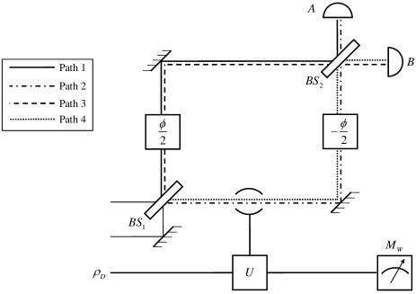
Figure 1: The Mach-Zehnder interferometer with an asymmetric beam splitter. The particle is prepared in an arbitrary state before entering the interferometer and after the first beam splitter two different phases are introduced. After the second beam splitter two counting detectors $A$ and $B$ record two interference patterns. The interference pattern recorded by the detector $A$ (the detector $B$) comes from path 1 and path 2 (path 3 and path 4). In addition, a WPD is introduced whose initial state is $\rho_{D}$. After interacting with the particle via a controlled unitary transformation, a special observable $W$ of the WPD is measured, from which the path information of the particle is inferred.

To obtain simultaneously the which-path information and the interference pattern, a WPD with initial state $\rho_{D}$ is coupled to the particle and two phase shifts $\pm\phi$ are introduced for the two paths $|0\rangle,|1\rangle$ respectively. The interaction between the particle and the WPD is effectively a controlled unitary transformation $\left|0\right\rangle\left\langle 0\right|\otimes I_{D}+\left|1\right\rangle\left\langle 1\right|\otimes U$ where $I_{D}$ and $U$ are the identity and a unitary operator act on the Hilbert space of the WPD. Thus the evolution of the particle and the detector after $BS_{1}$ is governed by the unitary operator

$$U_{QD}=e^{i\phi/2}\left|\varphi_{0}\right\rangle\left\langle 0\right|\otimes I_{D}+e^{-i\phi/2}\left|\varphi_{1}\right\rangle\left\langle 1\right|\otimes U$$ (3)

where $\left|\varphi_{0}\right\rangle\equiv B\left|0\right\rangle$ and $\left|\varphi_{1}\right\rangle\equiv B\left|1\right\rangle$. Let $\rho$ be the state of the particle after it has passed through $BS_{1}$. Then the final state of the whole system is described by

$$\rho_{f}^{(QD)} = U_{QD}(\rho\otimes\rho_{D})U_{QD}^{{\dagger}}$$ (4)

$$= \sum_{a,b=0}^{1}e^{i(b-a)\phi}|\varphi_{a}\rangle\langle a|\rho|b\rangle\langle\varphi_{b}|\otimes U^{a}\rho_{D}U^{\dagger b}.$$

III DISTINGUISHING TWO PATHS AMONG FOUR PATHS

First of all, we notice that the asymmetric beam splitter $BS_{2}$ can be regarded as a kind of which-path detector. Consider a simple case where the probabilities for the particle taking the two paths after $BS_{1}$ are equal, i.e., there is no a priori which-path knowledge. If the reflectivity $r$ of $BS_{2}$ is larger than $1/2$ and the particle is detected at the detector $A$, immediately one can infer that the particle passes more likely through the path $\left|0\right\rangle$. So the asymmetric beam splitter introduces additional a priori which-path knowledge and accordingly the visibility observed at the detector $A$ would be decreased. In a general case where the probabilities for taking the two paths after $BS_{1}$, namely $w_{+}=\left\langle 0\right|\rho\left|0\right\rangle$ and $w_{-}=\left\langle 1\right|\rho\left|1\right\rangle$, are not equal, the a priori which-path knowledge provided by $BS_{2}$ is different for a particle detected at one output port of the interferometer and a particle detected at the other output port. Accordingly, two different interference patterns emerge at the two output ports. Hence, in order to explore which path the particle passes through and to observe the interference pattern simultaneously, at first one should concentrate on particles detected at one output port and then choose a strategy to extract the which-path information from the measurements made on the detector, taking into account the corresponding a priori which-path knowledge.

Specifically, the introduction of an asymmetric beam splitter entails the need to distinguish two paths among four paths, see Fig. 1. On the observation of an interference pattern, e.g., at the detector $A$, two possible paths taken by the particles contributing to the interference are labeled with 1 and 2 respectively. When there is no WPD, the probabilities of taking the two paths are

$$w_{1}=\frac{rw_{+}}{rw_{+}+tw_{-}},\quad w_{2}=\frac{tw_{-}}{rw_{+}+tw_{-}},$$ (5)

which provides the conditional a priori which-path knowledge provided that detector $A$ fires. Similarly, for the particles detected by $B$, the probabilities of taking path 3 and path 4 are

$$w_{3}=\frac{tw_{+}}{rw_{-}+tw_{+}},\quad w_{4}=\frac{rw_{-}}{rw_{-}+tw_{+}}.$$ (6)

respectively. Note that (1) $w_{1,2}$ and $w_{3,4}$ are equal to $w_{\pm}$ when $BS_{2}$ is symmetric, and so to distinguish path 1 and path 2 (path 3 and path 4) is equivalent to distinguish the paths $\left|0\right\rangle$ and $\left|1\right\rangle$. Hence in a standard MZI scheme it is not necessary to involve four paths; (2) when $w_{\pm}=1/2$, the conditional a priori path information $w_{1,2}$ is the same as $w_{3,4}$, but not equal to $w_{\pm}$. In fact, in the experiment scheme in jacques only two paths need to be distinguished and the difference between $w_{\pm}$ and $w_{1,2}$ $(w_{3,4})$ is used to gain the which-path information. In other words, the asymmetric beam splitter in the experiment plays also the role of a WPD so that the path information and the interference pattern are obtained via the same detector. Thus the setup in jacques can be regarded as a standard MZI.

In the scheme we considered here, the predictability $\mathcal{P}$, the a priori fringe visibility $\mathcal{V}_{0}$, the visibility $\mathcal{V}$, and the distinguishability $\mathcal{D}$ must be defined particularly for each pair of paths. In what follows we shall consider only the interference pattern registered by detector $A$, and the case for the detector $B$ is similar. In this case the predictability of the paths 1 and 2 is obviously

$$\mathcal{P=}\left|w_{1}-w_{2}\right|.$$ (7)

The two paths taken by the particle are conditioned on the clicks in detector $A$, whose probability is given by

$$p\left(\phi\right) = \text{{tr}}_{QD}\left[|0\rangle\langle 0|\rho_{f}^{(QD)}\right]=rw_{+}+tw_{-}$$

$$+2\sqrt{rt}\left|\left\langle 0\right|\rho\left|1\right\rangle\text{{tr}}_{D}(\rho_{D}U)\right|\cos\left(\phi+\alpha+\delta\right),$$

where $\left\langle 0\right|\rho\left|1\right\rangle=\left|\left\langle 0\right|\rho\left|1\right\rangle\right|e^{i\alpha}$ and tr${}_{D}(\rho_{D}U)=|$tr${}_{D}(\rho_{D}U)|e^{-i\delta}$. If the WPD is not turned on, i.e, $U=I_{D}$, then the a priori visibility reads

$$\mathcal{V}_{0}=\frac{p_{\max}-p_{\min}}{p_{\max}+p_{\min}}=\frac{2\sqrt{rt}\left|\left\langle 0\right|\rho\left|1\right\rangle\right|}{rw_{+}+tw_{-}}.$$ (8)

It is easy to see that the well-known duality relation GY

$$\mathcal{P}^{2}+\mathcal{V}_{0}^{2}\leq 1$$ (9)

still holds in the present case. If the WPD is turned on, then the fringe visibility reads

$$\mathcal{V}=\mathcal{V}_{0}\left|\text{{tr}}_{D}\left(\rho_{D}U\right)\right|.$$ (10)

A general strategy $\mathcal{S}$ to guess the path taken by the particle is to divide the outcomes $W$ of the measurement of an observable $\hat{W}$ performed on the WPD into two disjoint sets, $S$ and $\bar{S}$. If $W\in S$, then one guesses the path to be 1; if $W\in\bar{S}$, then one guesses the path to be 2. The probability of guessing the right path is given by confluence

$$\mathcal{L}_{\hat{W},S}=w_{1}\sum_{W\in S}\left\langle W\right|\rho_{D}\left|W\right\rangle+w_{2}\sum_{W\in\bar{S}}\left\langle W\right|U\rho_{D}U^{{\dagger}}\left|W\right\rangle.$$ (11)

This is because once the particle is detected in path 1 (with probability $w_{1}$), the WPD will be in the state $\rho_{D}$; once the particle is detected in path 2 (with probability $w_{2}$), the WPD will be in the state $U\rho_{D}U^{{\dagger}}$. Let us denote

$$\eta_{S}\equiv\sum_{W\in S}\left\langle W\right|\rho_{D}\left|W\right\rangle,\quad\eta_{S}^{U}\equiv\sum_{W\in S}\left\langle W\right|U\rho_{D}U^{{\dagger}}\left|W\right\rangle,$$ (12)

together with $\eta_{\bar{S}}=1-\eta_{S}$ and $\eta_{\bar{S}}^{U}=1-\eta_{S}^{U}$. The which-path distinguishability for the given strategy $\mathcal{S}$ is then

$${\mathcal{D}}_{S}=2\mathcal{L}_{\hat{W},S}-1=2w_{1}\eta_{S}+2w_{2}\eta_{{S}}^{U}-1.$$ (13)

IV DUALITY RELATION FROM JOINT MEASURABILITY

The duality relation in an interferometer turns out to be intimately related to the joint measurement of two unsharp observables us . Generally, for a two-level system an unsharp observable is nothing else than a two-outcome positive-operator-valued measure (POVM). Two general unsharp observables $\left\{O_{\pm}\right\}$ and $\left\{O_{\pm}^{\prime}\right\}$ of a qubit take the form

$$O_{\pm}=\frac{I\pm\left(xI+\bm{m}\cdot\bm{\sigma}\right)}{2},\quad O_{\pm}^{\prime}=\frac{I\pm\left(yI+\bm{n}\cdot\bm{\sigma}\right)}{2}$$ (14)

where $I$ is the identity operator acting on the particle, and $\bm{\sigma}$ is the Pauli operator. The non-negativity imposes $\left|x\right|+\left|\bm{m}\right|\leq 1$ and so on. When $x=0$ and $\left|\bm{m}\right|=1$, $O_{\pm}$ are projectors of eigenstates of a sharp observable $\bm{m}\cdot\bm{\sigma}$. So, generally an unsharp observable is the smeared version of a sharp observable. The above two unsharp observables are jointly measurable if and only if there exists a joint unsharp observable $\{M_{\mu\nu}\}$ whose outcomes can be so grouped that the marginals correspond exactly to the two given unsharp observables, i.e.,

$$O_{\mu}=\sum_{\nu=\pm}M_{\mu\nu},\quad O_{\nu}^{\prime}=\sum_{\mu=\pm}M_{\mu\nu}.$$ (15)

If $y=0,$ then the necessary and sufficient condition for their joint measurability reads jm

$$\sqrt{\left(1+x\right)^{2}-\left|\bm{m}\right|^{2}}+\sqrt{\left(1-x\right)^{2}-\left|\bm{m}\right|^{2}}\geq\frac{2\left|\bm{m}\times\bm{n}\right|}{\sqrt{\left|\bm{m}\right|^{2}-(\bm{m}\cdot\bm{n})^{2}}}.$$ (16)

In our general MZI setup, the unsharp observable $\mathcal{N}=\{N_{0},N_{1}=I-N_{0}\}$ corresponding to the interference pattern registered in detector $A$ is given by $p(\phi)=$tr${}_{Q}(\rho N_{0})$ for an arbitrary $\rho$. Thus we obtain

$$N_{0}=\mathrm{tr}_{D}\left[U_{QD}^{{\dagger}}\left(\left|0\right\rangle\left\langle 0\right|\otimes I_{D}\right)U_{QD}\left(I\otimes\rho_{D}\right)\right]=\frac{I+{\bm{n}}\cdot\mathbf{\sigma}}{2}$$

with

$$\bm{n}=\left[2\frac{\mathcal{V}}{\mathcal{V}_{0}}\sqrt{rt}\cos\left(\phi+\delta\right),2\frac{\mathcal{V}}{\mathcal{V}_{0}}\sqrt{rt}\sin\left(\phi+\delta\right),2r-1\right].$$ (17)

For a given strategy ${\mathcal{S}},$ the probability of finding the detector in one of the eigenstates in $S$ is given by tr${}_{Q}(M_{S}\rho)$ for an arbitrary $\rho$ where

$$M_{S}=\sum_{W\in S}\text{{tr}}_{D}\left[U_{QD}^{{\dagger}}(I\otimes|W\rangle\langle W|)U_{QD}\left(I\otimes\rho_{D}\right)\right].$$

Thus the unsharp observable corresponding to the observable $\hat{W}$ and the strategy $\mathcal{S}$ is $\mathcal{M}=\{M_{S},I-M_{S}\}$ with

$$M_{S}=\frac{1}{2}\left[\left(\eta_{S}+\eta_{S}^{U}\right)I+\left(\eta_{S}-\eta_{S}^{U}\right)\sigma_{z}\right]=\frac{I+xI+\bm{m}\cdot{\bm{\sigma}}}{2},$$

in which notations in Eq. (12) have been used and

$$x=\eta_{S}+\eta_{S}^{U}-1,\quad\bm{m}=\left(0,0,\eta_{S}-\eta_{S}^{U}\right).$$ (18)

It is clear that as long as $r\neq 1/2$ we have $\bm{n\cdot m}\neq 0$, i.e., the two unsharp observables measured jointly in the general MZI setup are non-orthogonal, in contrast with a standard MZI setup us . From the joint measurement condition Eq. (16) it follows that

$$\sqrt{\eta_{S}\eta_{S}^{U}}+\sqrt{\eta_{\bar{S}}\eta_{\bar{S}}^{U}}\geq\frac{\mathcal{V}}{\mathcal{V}_{0}}.$$ (19)

Taking into the definition Eq. (13) and similar to the derivation in us , we obtain

$$\mathcal{D}_{\mathcal{S}}^{2}+\frac{1-\mathcal{P}^{2}}{\mathcal{V}_{0}^{2}}\mathcal{V}^{2}\leq 1-\gamma_{S}^{2},$$ (20)

where $\gamma_{S}=2\left|w_{1}\sqrt{\eta_{S}\eta_{\bar{S}}}-w_{2}\sqrt{\eta_{S}^{U}\eta_{\bar{S}}^{U}}\right|$. By maximizing over all possible strategies we obtain a duality inequality in the same form as Eq. (1).

V CONCLUSIONS AND DISCUSSIONS

We have considered how to illustrate quantitatively the wave-particle duality a general MZI scenario with an asymmetric beam splitter. The asymmetric beam splitter introduces additional a priori which-path knowledge which is different for a particle detected at one output port of the interferometer and a particle detected at the other, and consequently the fringe visibilities of the interference patterns at the two output ports are also different. Therefore, we should concentrate on particles detected at one output port and distinguish two possible paths taken by the particles detected at that port among four paths, and so our result is not a straight-forward extension of the duality inequality in a standard MZI set up with symmetric beam splitter. For each particle detected at the output port, a pair of unsharp observables are jointly measured. It turns out that non-orthogonality of the two unsharp observables is caused by the asymmetric beam splitter, which characterizes the general MZI setup. We have employed the condition for joint measurability of the two unsharp observables to obtain a duality inequality.

It would be interesting to ask what is the experimental setup to measure jointly a pair of most general unsharp observables of a two-level system, though the condition for their jointly measurability has been established jm . Reversely, whether does the most general jointly measurability condition imply a “thorough” complementarity relation with realizable and observable effects not limited by the known duality inequalities? These questions remain open for further research. The answers may lead to a device-independent duality inequality.

- (1) N. Bohr, Nature (London) 121, 580 (1928).
- (2) W. K. Wootters and W. H. Zurek, Phys. Rev. D 19, 473 (1979).
- (3) D. M. Greenberger and A. Yasin, Phys. Lett. A 128, 391 (1988).
- (4) G. Jaeger, A. Shimony, and L. Vaidman, Phys. Rev. A 51, 54 (1995).
- (5) B.-G. Englert, Phys. Rev. Lett. 77, 2154 (1996).
- (6) B.-G. Englert and J. A. Bergou, Opt. Commun. 179, 337 (2000).
- (7) H. Martens and W. M. de Muynck, Found. Phys. 20, 255 (1990).
- (8) W. M. de Muynck, Foundations of Quantum Mechanics: An Empiricist Approach (Kluwer Academic Publishers, Dordrecht, 2002).
- (9) P. Busch, Phys. Rev. D 33, 2253 (1986).
- (10) P. Busch and C. Shilladay, Phys. Rep. 435, 1 (2006).
- (11) Y. Kurotani, T. Sagawa, and M. Ueda, Phys. Rev. A 76, 022325 (2007).
- (12) T. Sagawa and M. Ueda, Phys. Rev. A 77, 012313 (2008).
- (13) P. Busch and T. Heinosaari, Quantum Inf. Comp. 8, 0797 (2008).
- (14) T. Heinosaari, P. Stano, and D. Reitzner, Int. J. Quantum Inf. 6, 975 (2008).
- (15) N.-L. Liu, L. Li, S. Yu, and Z.-B. Chen, Phys. Rev. A 79, 052108 (2009).
- (16) P. Stano, D. Reitzner, and T. Heinosaari, Phys. Rev. A 78, 012315 (2008).
- (17) S. Yu, N.-L. Liu, L. Li, and C. H. Oh, Phys. Rev. A 81, 062116 (2010).
- (18) P. Busch and H.-J. Schmidt, Quant. Info. Proc. 9, 143 (2010).
- (19) E. Andersson, S. M. Barnett, and A. Aspect, Phys. Rev. A 72, 042104 (2005).
- (20) T. Brougham, E. Andersson, and S. M. Barnett, Phys. Rev. A 80, 042106 (2009).
- (21) T. Brougham, E. Andersson, and S. M. Barnett, Phys. Rev. A 73, 062319 (2006).
- (22) A. Ferraro and M. G. A. Paris, Open Sys. & Information Dyn. 14, 149 (2007).
- (23) M. M. Wolf, D. Perez-Garcia, and C. Fernandez, Phys. Rev. Lett. 103, 230402 (2009).
- (24) V. Jacques, E. Wu, F. Grosshans, F. Treussart, P. Grangier, A. Aspect, and J. F. Roch, Phys. Rev. Lett. 100, 220402 (2008).
- (25) To see which path dose the particle actully pass through, in standard MZI other two detectors can be directly set on the two paths and . The conflunce of the paths 1 and 2 after makes this method inavailable. However, in principle one can still accomplish it with distinguishing another freedom of the particle. As an example, polarization is used in englert exp .
- (26) P. D. D. Schwindt, P. G. Kwiat, and B.-G. Englert, Phys. Rev. A 60, 4285 (1999).