Spontaneous symmetry breaking of binary fields in a nonlinear double-well structure

Abstract

We introduce a one-dimensional two-component system with the self-focusing cubic nonlinearity concentrated at a symmetric set of two spots. Effects of the spontaneous symmetry breaking (SSB) of localized modes were previously studied in the single-component version of this system. In this work, we study the evolution (in the configuration space of the system) and SSB scenarios for two-component modes of three generic types, as concerns the spatial symmetry of each component: symmetric-symmetric (Sm-Sm), antisymmetric-antisymmetric (AS-AS), and symmetric-antisymmetric (S-AS) ones. In the limit case of the nonlinear potential represented by two $\delta$-functions, solutions are obtained in a semi-analytical form. They feature novel properties, in comparison with the previously studied single-component model. In particular, the SSB of antisymmetric modes is possible solely in the two-component system, and, obviously, S-AS states exist only in the two-component system too. In the general case of the symmetric pair of finite-width nonlinear potential wells, evolution scenarios are very complex. In this case, new results are reported, first, for the single-component model. These are pairs of broken-antisymmetry modes, and of twin-peak symmetric ones, which are generated by saddle-mode bifurcations separated from the transformations previously studied in the the single-component setting. With regard to these findings, complex scenarios of the evolution of the two-component solution families are realized in terms of links connecting pairs of modes of three simplest types: (A) two-component ones with unbroken symmetries; (B) single-component modes featuring density peaks in both potential wells; (C) single-component modes which are trapped, essentially, in a single well.

I Introduction and the model

A fundamental effect caused by the interplay of nonlinearity with symmetric potentials is spontaneous symmetry breaking (SSB). The simplest setting where this effect occurs is represented by double-well potentials. A commonly known property of one-dimensional quantum mechanics is that the ground state shares the symmetry of the underlying double-well potential LL . If the self-attractive cubic nonlinearity is added to the consideration, the corresponding Schrödinger equation is transformed into the Gross-Pitaevskii equation for a Bose-Einstein condensate (BEC) loaded into the double-well potential BEC , or the nonlinear Schrödinger equation for photonic counterparts of the system NLS . The nonlinear term may break the symmetry of the ground state, replacing it by an asymmetric one which minimizes the energy of the system, provided that the strength of the nonlinearity exceeds a certain critical value (see Ref. misc for the general analysis, and Ref. misc2 for the consideration of the SSB of self-trapped states in BEC). The experimental realization of the SSB in double-well potentials was reported in BEC Markus (this was done in the condensate with the self-repulsive nonlinearity, which implies the spontaneous breaking of the antisymmetry of the lowest-energy antisymmetric mode) and in nonlinear optics photo .

The symmetry-breaking bifurcation, which destabilizes the original symmetric ground state and gives rise to the SSB in the nonlinear systems, was originally predicted in a discrete model of self-trapping Chris . In nonlinear optics, a similar bifurcation was analyzed in Ref. Snyder for continuous-wave (spatially uniform) light signals in dual-core fibers. The allied bifurcation for solitons in nonlinear dual-core fibers was studied in detail in Ref. dual-core . Later, the SSB was studied for gap solitons in the model of the dual-core fiber Bragg gratings with the same cubic nonlinearity as in the ordinary fibers Mak . The SSB effects were also predicted for matter-wave solitons in the self-attractive BEC loaded into a double-channel potential trap Arik -Luca .

Typically, the self-attractive cubic nonlinearity gives rise to the soliton bifurcations of the subcritical (backward) type (in other words, these are phase transitions of the first kind). In that case, branches of asymmetric modes emerge as unstable ones, going backward (i.e., in the direction of the decrease of the soliton’s norm (energy)). They get stabilized after switching the evolution direction forward at turning points of the bifurcation diagram bif . It was also demonstrated that the combination of the self-focusing nonlinearity with a periodic potential applied in the free direction (perpendicular to the direction of the action of the double-well potential) tends to change the character of the soliton bifurcation from sub- to supercritical (i.e., replace the phase transition of the first kind by a transition of the second kind). In the supercritical case, the asymmetric branches emerge as stable ones, going in the forward direction, i.e., in the direction of the increase of the soliton’s norm Arik ; Warsaw2 . The bifurcation for gap solitons in the dual-core fiber Bragg grating is of the forward type too Mak .

A challenging alternative to the use of the ordinary linear double-well potential is the setting based on an effective nonlinear potential, alias pseudopotential (as it is called in solid-state physics Harrison ), which is induced by the double-peak spatial modulation of the local strength of the self-focusing nonlinearity. Pseudopotentials featuring the double-well shape can be realized in optics and matter waves Pu ; Barcelona . The ultimate form of such a setting is the one with the nonlinearity concentrated at two points, represented by a symmetric pair of delta-functions or narrow Gaussians Dong ; Nir (the simplest model of that type, with the self-attractive nonlinearity represented by a single delta-function, was first introduced in Ref. Mark ). Two-dimensional counterparts of the system were considered too, in the form of two parallel channels Hung , or two symmetric circles new , in which the self-attractive nonlinearity is localized . The SSB of solitons in the symmetric nonlinear double-well potentials was studied in detail, featuring the subcritical type of the symmetry breaking Dong ; Hung ; Nir .

It is relevant to mention that SSB effects were also analyzed for discrete solitons in dual-core nonlinear chains, with the uniform linear coupling between them Herring , as well as with the linear coupling which links a single pair of sites in the parallel chains Ljupco . The form of the linear coupling determines the type of the respective SSB bifurcation, which is subcritical in the former case, and supercritical in the latter situation. The action of the nonlinearity concentrated at a pair of sites embedded into a single linear chain was studied too Molina ; Valera . The SSB effects in this setting (for both straight and circular host linear chains) were analyzed in recent work Valera . The SSB in a similar system, with a pair of symmetric nonlinear sites side-coupled to the infinite linear chain, was recently studied in Ref. Almas .

An obviously relevant generalization of the work outlined above is extension to two-component systems. In BEC, this implies a mixture of two different hyperfine states of the same atomic species BEC , while in optics it implies the co-propagation of light beams mixing two different polarizations of light, or different carrier wavelengths. Recently, the SSB, along with the related dynamical effect of Josephson oscillations between the wave functions trapped in adjacent potential wells, have been analyzed in diverse models of binary systems embedded into ordinary (linear) potentials of the double-well type binarySSB . An experiment was performed too, for the corresponding BEC mixture Markus2 . However, SSB effects have not yet been studied in two-component systems trapped in double-well nonlinear (pseudo)potentials. A straightforward possibility to implement the latter setting can be found in nonlinear optics, where the spatially nonuniform nonlinearity, which forms the double-well structure, will act similarly on both polarization components, in the form of the SPM (self-phase modulation), as well as on the XPM (cross-phase-modulation) nonlinear interaction between them NLS .

In this work, we aim to perform the analysis of the two-component system in the nonlinear double-well potential, with emphasis on manifestations of the SSB in the two-component mixture. To this end, we aim to consider the basic setting with the symmetric pair of strongly localized nonlinear spots embedded into the one-dimensional linear host medium. Thus, our model is the generalization, for wave functions $\phi(x,t)$ and $\psi(x,t)$ of the two components, of the single-component model introduced in Ref. Dong :

$$i\phi_{t} = -\frac{1}{2}\phi_{xx}+g(x)\left(|\phi|^{2}+G\left|\psi\right|^{2}\right)\phi,$$ (1)

$$i\psi_{t} = -\frac{1}{2}\psi_{xx}+g(x)\left(|\psi|^{2}+G\left|\phi\right|^{2}\right)\psi,$$ (2)

where $G>0$ is the relative strength of the XPM nonlinearity, while the SPM coefficient is normalized to be $1$. In the optical model corresponding to these equations, the evolutional variable $t$ is actually the propagation distance (usually denoted as $z$), while $x$ is the transverse coordinate (in the BEC model, $t$ is simply time). As for the XPM coefficient, its typical values in optics are $G=2/3$ for the coupled linear polarizations, and $G=2$ for the pair of orthogonal polarizations or different carrier wavelengths NLS . Other values of $G$ are also possible, for elliptically polarized beams.

Following Ref. Dong , the nonlinearity-modulation function in Eqs. (1) and (2), which corresponds to the symmetric set of two strongly localized nonlinear spots, is adopted in the form of

$$g(x)=-\frac{1}{a\sqrt{\pi}}\left[\exp\left(-\frac{\left(x+1\right)^{2}}{a^{2}}\right)+\exp\left(-\frac{\left(x-1\right)^{2}}{a^{2}}\right)\right]\,,$$ (3)

which is subject to the normalization condition,

$$\int_{-\infty}^{+\infty}g(x)dx\leavevmode\nobreak\ \equiv-2.$$ (4)

Profiles of modulation function (3), which keeps the double-well structure at $a<\sqrt{2}$, are shown, for different values of $a$, in Fig. 1.

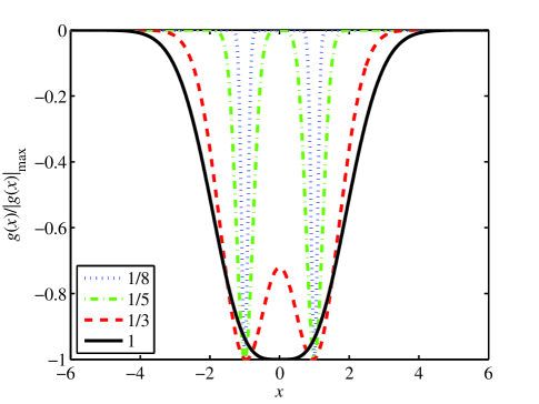
Figure 1: (Color online) Shapes of the double-well nonlinearity-modulation function (3), normalized to its maximum value, are shown (as per Ref. Dong ) for different values of scaled width $a$ of the individual well.

Equations (1) and (2) conserve three dynamical invariants, viz., two norms and the energy (Hamiltonian),

$$M \equiv \int_{-\infty}^{+\infty}|\phi(x)|^{2}dx,\leavevmode\nobreak\ N\equiv\int_{-\infty}^{+\infty}|\psi(x)|^{2}dx,\leavevmode\nobreak\$$ (5)

$$H = \frac{1}{2}\int_{-\infty}^{\infty}\left[\left|\phi_{x}\right|^{2}+\left|\psi_{x}\right|^{2}+g(x)\left(\left|\phi\right|^{4}+\left|\psi\right|^{4}+2G\left|\phi\right|^{2}\left|\psi\right|^{2}\right)\right]dx.$$ (6)

Stationary localized solutions to Eqs. (1) and (2) are sought for as $\phi=e^{-i\lambda t}u(x),\leavevmode\nobreak\ \psi=e^{-i\mu t}v(x)$, where the chemical potentials of localized modes must be negative, $\lambda<0$, $\mu<0$, and real functions $u(x)$ and $v(x)$ satisfy equations

$$\lambda u+\frac{1}{2}u^{\prime\prime}+\frac{1}{a\sqrt{\pi}}\left[\exp\left(-\frac{\left(x+1\right)^{2}}{a^{2}}\right)+\exp\left(-\frac{\left(x-1\right)^{2}}{a^{2}}\right)\right]\left(u^{2}+Gv^{2}\right)u = 0,$$ (7)

$$\mu v+\frac{1}{2}v^{\prime\prime}+\frac{1}{a\sqrt{\pi}}\left[\exp\left(-\frac{\left(x+1\right)^{2}}{a^{2}}\right)+\exp\left(-\frac{\left(x-1\right)^{2}}{a^{2}}\right)\right]\left(v^{2}+Gu^{2}\right)v = 0$$ (8)

A special version of the model corresponds to the limit of $a\rightarrow 0$, with Eqs. (7) and (8) going over into

$$\lambda u = -(1/2)u^{\prime\prime}-\left[\delta(x+1)+\delta(x-1)\right]\left(u^{2}+Gv^{2}\right)u,$$ (9)

$$\mu v = -(1/2)v^{\prime\prime}-\left[\delta(x+1)+\delta(x-1)\right]\left(v^{2}+Gu^{2}\right)v,$$ (10)

where $\delta(x)$ is the Dirac’s delta-function.

To conclude the Introduction, it is relevant to mention that a two-field model with a symmetric set of two strongly localized nonlinear spots was recently introduced for the quadratic (second-harmonic-generating) optical nonlinearity Asia . In the limit case when the nonlinearity profile is described by the pair of $\delta$-functions, cf. Eqs. (9) and (10), the corresponding equations for the complex amplitudes of the fundamental-frequency and second-harmonic waves, $U(x,z)$ and $V\left(x,z\right)$, take the form of

$$iU_{z}+(1/2)U_{xx}+\delta(x)U^{\ast}V = 0,$$

$$2iV_{z}+(1/2)V_{xx}-QV+(1/2)\delta(x)U^{2} = 0,$$

where the asterisk stands for the complex conjugate, $z$ is the propagation distance, and real constant $Q$ measures the mismatch frustrating the parametric interaction between the two waves. Although involving the two wave fields, this system (for which exact solutions for symmetric, antisymmetric, and asymmetric localized modes have been found in Ref. Asia ) is actually closer to the single-component model in the case of the cubic nonlinearity, due to the coherent character of the nonlinear coupling between the waves $U$ and $V$. In particular, system (LABEL:UV) directly reduces to its single-component cubic counterpart in the cascading limit, which corresponds to large positive values of $Q$.

The rest of the paper is organized as follows. The limit case of the two-component system with the modulation profile based on the set of $\delta$-functions, which corresponds to Eqs. (9) and (10), is considered in detail in Section 2 (in the beginning of the section, we also give an exact solution for the two-component system with the single nonlinear $\delta$-function, as this simple case was not considered previously). The system with the pair of $\delta$-functions admits a semi-analytical solution, which reduces to a system of four coupled cubic algebraic equations for amplitudes of asymmetric modes, while symmetric (Sm) and antisymmetric (AS) ones can be found in a fully analytical form.

In Section 3, we report results of the analysis of the two-component model in the general case, corresponding to the nonlinearity-modulation function (3) with finite $a$. In that case, the analysis is based on a comprehensive numerical solution of ODEs (7) and (8) with $a>0$. The consideration in Section 3 starts by revisiting the single-component model, with the aim to report additional solutions of the Sm and broken-AS types (the latter means modes with broken antisymmetry). These solutions were not reported in Ref. Dong , as they represent pairs of modes generated by saddle-node bifurcations which occur at sufficiently large $a$, being detached from the branches which continuously evolve from the limit case of $a\rightarrow 0$. The subsequent analysis of the two-component system reported in Section 3 produces a full picture of bifurcations for compound modes of the Sm-Sm (symmetric-symmetric), AS-AS (antisymmetric-antisymmetric), and S-AS (symmetric-antisymmetric) types, and their broken counterparts, i.e., modes with spontaneously broken (anti)symmetries. Because the full picture turns out to be extremely complex, we report only parts of it, which may be presented in a relatively simple form. Despite the complexity of the picture, some underlying principles can be formulated in a general form: the fundamental role is played by simplest solutions, namely the two-component unbroken modes (i.e., those with the unbroken (anti)symmetries), and single-component solutions of both the unbroken and broken types. As a matter of fact, numerous families of two-component solutions, which feature sophisticated evolution in the system’s configuration space, may be understood as branches linking various pairs of these simplest modes (the complexity is often produced by the fact that the branches make one or several loops, in the course of their evolution).

The paper is concluded by Section 4. In particular, we discuss the necessity of the systematic analysis of the dynamical stability of the diverse stationary modes found in this work. With a few exceptions, we do not analyze the stability here, as the study of the stationary modes and their bifurcations is by itself a sufficiently heavy topic for a single paper.

II The model with the delta-functions ($a\rightarrow 0$)

II.1 The single delta-function

Before presenting results for the model with the symmetric pair of $\delta$-functions, it makes sense to briefly consider the case of the nonlinearity represented by the single $\delta$-function, when Eqs. (1) and (2) are replaced by

$$i\phi_{t} = -\frac{1}{2}\phi_{xx}+\delta(x)\left(|\phi|^{2}+G\left|\psi\right|^{2}\right)\phi,$$ (12)

$$i\psi_{t} = -\frac{1}{2}\psi_{xx}+\delta(x)\left(|\psi|^{2}+G\left|\phi\right|^{2}\right)\psi,$$ (13)

and, accordingly, their stationary version, Eqs. (9) and (10), is replaced by

$$\lambda u = -(1/2)u^{\prime\prime}-\delta(x)\left(u^{2}+Gv^{2}\right)u,$$ (14)

$$\mu v = -(1/2)v^{\prime\prime}-\delta(x)\left(v^{2}+Gu^{2}\right)v.$$ (15)

It is straightforward to find solutions to Eqs. (14) and (15) with both fields different from zero:

$$\left\{u(x),v(x)\right\} = \left\{A,B\right\}\exp\left(-\sqrt{-2\left\{\lambda,\mu\right\}}|x|\right),$$ (16)

$$\left\{A^{2},B^{2}\right\} = \frac{\sqrt{2}}{G^{2}-1}\left(G\sqrt{-\left\{\mu,\lambda\right\}}-\sqrt{-\left\{\lambda,\mu\right\}}\right).$$ (17)

These solutions exist for $G\neq 1$ ($G=1$ is the degenerate case corresponding to the Manakov’s nonlinearity NLS ), for negative chemical potentials $\lambda$ and $\mu$, in the regions of

$$\frac{1}{G} < \sqrt{\frac{\lambda}{\mu}}<G,\leavevmode\nobreak\ \leavevmode\nobreak\ \mathrm{if}\leavevmode\nobreak\ \leavevmode\nobreak\ G>1,$$ (18)

$$G < \sqrt{\frac{\lambda}{\mu}}<\frac{1}{G},\leavevmode\nobreak\ \leavevmode\nobreak\ \mathrm{if}\leavevmode\nobreak\ \leavevmode\nobreak\ G<1.$$ (19)

It is also instructive to cast Eq. (17) into the form of relations between the chemical potentials and norms $M$ and $N$ of the two components (see Eq. (5)). Obviously, $\left\{M,N\right\}=\left\{A^{2},B^{2}\right\}/\sqrt{-2\left\{\lambda,\mu\right\}}$ for solutions (16), hence

$$\left\{M,N\right\}=\frac{1}{G^{2}-1}\left(G\sqrt{\left\{\frac{\mu}{\lambda},\frac{\lambda}{\mu}\right\}}-1\right).$$ (20)

Although we chiefly leave the issue of the dynamical stability aside in this paper, Eq. (20) makes it possible to address the stability problem, using the Vakhitov-Kolokolov (VK) criterion. It states that, for the single-component model, with the soliton family characterized by dependence $M=M(\lambda)$, the necessary stability condition is $dM/d\mu\leq 0$ VK ; Berge' , while for the two-component model with separately conserved norms and two independent chemical potentials the switch between the stability and instability occurs at points where the corresponding Jacobian determinant vanishes:

$$J\left(\lambda,\mu\right)\equiv\left\|\frac{\partial\left(M,N\right)}{\partial\left(\lambda,\mu\right)}\right\|=0.$$ (21)

In the single-component model with the single nonlinear $\delta$-function, the soliton family is degenerate, in the sense that its norm does not depend on the chemical potential: $M\equiv 1$, hence this family seems as a neutrally-stable one, which actually does not guarantee the true stability. In reality, the single-component family was found to be completely unstable Nir . In the present case, the calculation of Jacobian $J\left(\lambda,\mu\right)$ for the two-component solitons per Eq. (20) demonstrates that this determinant identically vanishes, $J\left(\lambda,\mu\right)\equiv 0$, suggesting that the total family of solutions (16), (17) is completely unstable too. Indeed, one can easily find the following set of exact nonstationary solutions to Eqs. (12) and (13), with arbitrary real constant $\alpha$ and $\beta$:

$$\left\{\phi\left(x,t\right)\psi(x,t)\right\} = \left\{\alpha,\beta\right\}|t|^{-1/2}\exp\left[\frac{i}{2t}\left(|x|-i\left\{a,b\right\}\right)^{2}\right],$$ (22)

$$\left\{a,b\right\} \equiv -\left(\left\{\alpha^{2},\beta^{2}\right\}+G\left\{\beta^{2},\alpha^{2}\right\}\right)\mathrm{sgn}(t),$$ (23)

which generalize similar exact single-component solutions found in Ref. Nir . At $t<0$, solutions (22), (23) describe the collapse of the perturbed soliton (the formation of a singularity at $x=0$), which happens at $t\rightarrow-0$, while at $t>0$ the solution describes decay of the soliton. Thus, the nonstationary solutions demonstrate that the solitons belonging to the degenerate family (16), (17), supported by the single $\delta$-function, suffer either the collapse or decay, being indeed unstable, as conjectured above. On the other hand, we expect that the replacement of the ideal $\delta$-functions by a finite-width profile may stabilize the solutions, cf. Ref. KaiLi where this was demonstrated for the single-component model.

II.2 Amplitude equations for the system with two delta-functions

Proceeding to the model with the symmetric set of two $\delta$-functions, based on Eqs. (9) and (10), our first objective is to obtain analytical results, following the pattern of Ref. Dong , where a full analytical solution was found for stationary states in the corresponding single-component model. Off points $x=\pm 1$, equations (9) and (10) are linear, a general solution to which, decaying at $|x|\rightarrow\infty$, can be sought for as

$$u(x)=\left\{\begin{array}[]{c}B_{1}e^{\sqrt{2|\lambda|}\left(x+1\right)},\leavevmode\nobreak\ \mathrm{at}\leavevmode\nobreak\ x<-1,\\ A_{0}e^{-\sqrt{2|\lambda|}\left(x-1\right)}+B_{0}e^{\sqrt{2|\lambda|}\left(x+1\right)},\leavevmode\nobreak\ \mathrm{at}\leavevmode\nobreak\ -1<x<+1,\\ A_{1}e^{-\sqrt{2|\lambda|}\left(x-1\right)},\leavevmode\nobreak\ \mathrm{at}\leavevmode\nobreak\ x>+1,\end{array}\right.$$ (24)

$$v(x)=\left\{\begin{array}[]{c}D_{1}e^{\sqrt{2|\mu|}\left(x+1\right)},\leavevmode\nobreak\ \mathrm{at}\leavevmode\nobreak\ x<-1,\\ C_{0}e^{-\sqrt{2|\mu|}\left(x-1\right)}+D_{0}e^{\sqrt{2|\mu|}\left(x+1\right)},\leavevmode\nobreak\ \mathrm{at}\leavevmode\nobreak\ -1<x<+1,\\ C_{1}e^{-\sqrt{2|\mu|}\left(x-1\right)},\leavevmode\nobreak\ \mathrm{at}\leavevmode\nobreak\ x>+1,\end{array}\right.$$ (25)

with constant amplitudes $A_{0},A_{1}$, $B_{0},B_{1}$ and $C_{0},C_{1},\leavevmode\nobreak\ D_{0},D_{1}$. The continuity of the wave functions at $x=\pm 1$ imposes four relations on the amplitudes,

$$B_{1} = B_{0}+A_{0}e^{2\sqrt{2|\lambda|}},\leavevmode\nobreak\ A_{1}=A_{0}+B_{0}e^{2\sqrt{2|\lambda|}},$$ (26)

$$D_{1} = D_{0}+C_{0}e^{2\sqrt{2|\mu|}},\leavevmode\nobreak\ C_{1}=C_{0}+D_{0}e^{2\sqrt{2|\mu|}}.$$ (27)

Using these relations, one may eliminate “inner” amplitudes $A_{0}$,$B_{0},C_{0},D_{0}$ in favor of their “outer” counterparts $A_{1}$,$B_{1},C_{1},D_{1}$:

$$A_{0} = \frac{e^{2\sqrt{2|\lambda|}}B_{1}-A_{1}}{e^{4\sqrt{2|\lambda|}}-1},\leavevmode\nobreak\ B_{0}=\frac{e^{2\sqrt{2|\lambda|}}A_{1}-B_{1}}{e^{4\sqrt{2|\lambda|}}-1},$$ (28)

$$C_{0} = \frac{e^{2\sqrt{2|\mu|}}D_{1}-B_{1}}{e^{4\sqrt{2|\mu|}}-1},\leavevmode\nobreak\ D_{0}=\frac{e^{2\sqrt{2|\mu|}}C_{1}-D_{1}}{e^{4\sqrt{2|\mu|}}-1}$$ (29)

Further, the integration of Eqs. (9) and (10) in infinitesimal vicinities of points $x=\pm 1$ yields expressions for jumps ($\Delta$) of the first derivative at these points,

$$\Delta\left(u^{\prime}\right)|_{x=\pm 1} = -2\left[\left(u|_{x=\pm 1})^{2}+G(v|_{x=\pm 1}\right)^{2}\right],$$ (30a)

$$\Delta\left(v^{\prime}\right)|_{x=\pm 1} = -2\left[\left(v|_{x=\pm 1})^{2}+G(u|_{x=\pm 1}\right)^{2}\right].$$ (30b)

The substitution of solution (24) and (25) into relations (30) leads to a system of equations for the outer amplitudes,

$$\sqrt{|\lambda|/2}\left(B_{1}-B_{0}+A_{0}e^{2\sqrt{2|\lambda|}}\right) = \left(B_{1}^{2}+GD_{1}^{2}\right)B_{1},$$ (31)

$$\sqrt{|\lambda|/2}\left(A_{1}-A_{0}+B_{0}e^{2\sqrt{2|\lambda|}}\right) = \left(A_{1}^{2}+GC_{1}^{2}\right)A_{1}.$$ (32)

$$\sqrt{|\mu|/2}\left(D_{1}-D_{0}+C_{0}e^{2\sqrt{2|\mu|}}\right) = \left(D_{1}^{2}+GB_{1}^{2}\right)D_{1},$$ (33)

$$\sqrt{|\mu|/2}\left(C_{1}-C_{0}+D_{0}e^{2\sqrt{2|\mu|}}\right) = \left(C_{1}^{2}+GA_{1}^{2}\right)C_{1}.$$ (34)

After the substitution of expressions (28) and (29) into Eqs. (32)-(34), we end up with a system of four coupled cubic equations for $A_{1}$,$B_{1}$,$C_{1},D_{1}$:

$$\sqrt{|\lambda|/2}\left(e^{2\sqrt{2|\lambda|}}B_{1}-A_{1}\right)=\sinh\left(2\sqrt{2|\lambda|}\right)\left(B_{1}^{2}+GD_{1}^{2}\right)B_{1},$$ (35)

$$\sqrt{|\lambda|/2}\left(e^{2\sqrt{2|\lambda|}}A_{1}-B_{1}\right)=\sinh\left(2\sqrt{2|\lambda|}\right)\left(A_{1}^{2}+GC_{1}^{2}\right)A_{1}.$$ (36)

$$\sqrt{|\mu|/2}\left(e^{2\sqrt{2|\mu|}}D_{1}-C_{1}\right)=\sinh\left(2\sqrt{2|\mu|}\right)\left(D_{1}^{2}+GB_{1}^{2}\right)D_{1},$$ (37)

$$\sqrt{|\mu|/2}\left(e^{2\sqrt{2|\mu|}}C_{1}-D_{1}\right)=\sinh\left(2\sqrt{2|\mu|}\right)\left(C_{1}^{2}+GA_{1}^{2}\right)C_{1}.$$ (38)

Symmetric solutions to Eqs. (35)-(38) (as said above, they will be referred to as “Sm-Sm” modes, i.e., those which are spatially symmetric in each component) are looked for by setting $A_{1}=B_{1}$ and $C_{1}=D_{1}$, which reduces the system to equations

$$A_{1}^{2}+GC_{1}^{2} = \frac{\sqrt{2|\lambda|}}{1+e^{-2\sqrt{2|\lambda|}}},$$ (39a)

$$C_{1}^{2}+GA_{1}^{2} = \frac{\sqrt{2|\mu|}}{1+e^{-2\sqrt{2|\mu|}}}.$$ (39b)

Similarly, solutions to Eqs. (35)-(38) which are antisymmetric in each component (“AS-AS” states) are looked for with $$A_{1}=-B_{1} C_{1}=-D_{1}$$ and , reducing Eqs. (35)-(38) to

$$A_{1}^{2}+GC_{1}^{2} = \frac{\sqrt{2|\lambda|}}{1-e^{-2\sqrt{2|\lambda|}}},$$ (40a)

$$C_{1}^{2}+GA_{1}^{2} = \frac{\sqrt{2|\mu|}}{1-e^{-2\sqrt{2|\mu|}}}.$$ (40b)

There also exist solutions to Eqs. (35)-(38) with mixed symmetry, e.g., antisymmetric in component $u$ and symmetric in $v$, which implies $A_{1}=-B_{1}$ and $C_{1}=D_{1}$ (“S-AS” states). This restriction reduces the system of Eqs. (35)-(38) to a simplified one,

$$A_{1}^{2}+GC_{1}^{2} = \frac{\sqrt{2|\lambda|}}{1-e^{-2\sqrt{2|\lambda|}}},$$ (41a)

$$C_{1}^{2}+GA_{1}^{2} = \frac{\sqrt{2|\mu|}}{1+e^{-2\sqrt{2|\mu|}}}.$$ (41b)

II.3 Analysis of the solutions

Systems (39), (40) and (41) are obviously analytically solvable, as each one is tantamount to a system of two inhomogeneous linear equations for $A_{1}^{2}$ and $C_{1}^{2}$, while the general algebraic system (35)-(38) can be only solved in a numerical form. Norms (5) and energy (6) for the solutions were also calculated numerically, because analytical expressions for these integrals are very cumbersome (they are actually analytically intractable even in the single-component model Dong ). The results are displayed below for $G=2$. As said above, in optics models this value corresponds to the interaction between orthogonal circular polarizations, or between waves with different carrier wavelengths.

The numerical solutions reveals a plethora of different branches of the localized modes, with different degrees of the asymmetry. Typical examples of the corresponding spatial models of the different types are presented in Fig. 2. In this paper, we aim to report only a part of the results, which represent the most characteristic findings, that may be presented in a sufficiently clear form, as the full description of the (anti)symmetry breaking in the two-component model (both for $a\rightarrow 0$ and finite $a$) is extremely complex. Generally, the results may be understood as those pertaining to modes generated by the spontaneous (anti)symmetry breaking from the above-mentioned solutions of three special types, i.e., Sm-Sm, AS-AS, and S-AS ones. This is the principal difference from the single-component model, where asymmetric modes could be generated solely from the symmetric ones (antisymmetric states were dynamically unstable at small $a$ and stable at larger $a,$ but they never underwent a symmetry-breaking bifurcation).

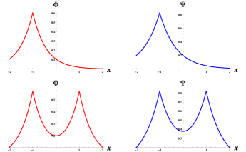
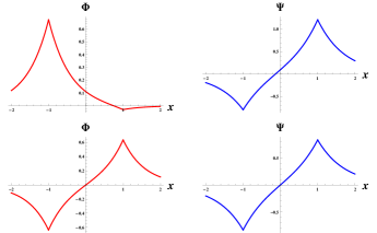
(a)        (b) (c)

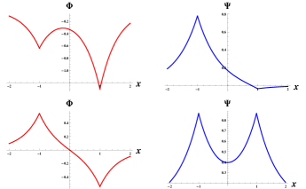
Figure 2: (Color online) Typical examples of the exact modes in the model with two $\delta$-functions, produced by solution of algebraic equations (35)-(38) at $\lambda=1.5$ and $\mu=1.0$: Sm-Sm modes (a), AS-AS modes (b), and S-AS modes (c), each with broken and unbroken (anti)symmetry.

Each species of the modes may be characterized by their energy (6) and spatial asymmetries of the two fields, which are defined as follows:

$$\Delta\Theta_{\left\{\phi,\psi\right\}}\equiv\frac{1}{\left\{M,N\right\}}\left(\int\limits_{0}^{+\infty}dx\left|\left\{\phi(x),\psi(x\right\})\right|^{2}-\int\limits_{-\infty}^{0}dx\left|\left\{\phi(x),\psi(x)\right\}\right|^{2}\right).$$ (42)

Exacerbating the complexity of the results, there is, in general, no one-to-one relation between chemical potentials $\mu$,$\nu$ and norms $M,N$, as well as total energy $H$, see Eqs. (5), (6). However, the asymmetries and energy of the solutions smoothly depend on $M$ and $N$, allowing us to classify the solutions according to the type of their (a)symmetry (Sm-Sm, AS-AS, S-AS, and their “broken” versions).

II.3.1 Solutions obtained from the symmetric-symmetric modes (Sm-Sm type)

We start by the presentation of the results for modes generated by the SSB of the states of the Sm-Sm type, as this case admits direct comparison with the results obtained for the SSB of the symmetric mode in the single-component model Dong . Examples of the symmetric modes with the broken and unbroken symmetry are shown in Fig. 2(a), for $\lambda=1.5$ and $\mu=1.0$. In Fig. 3, the asymmetry of one component of the “broken” solutions of the Sm-Sm type is displayed, along with total energy (6), considered as functions of norms (5). The asymmetry of the second component actually follows the same pattern.

A characteristic feature of the solutions of the Sm-Sm type, both “broken” and “unbroken” ones, is that they allow to establish a one-to-one correspondence between the norms and chemical potentials of the two components. It can be checked that both the norms and total energy (6) of these modes grow monotonously with the increase of $|\lambda|$ and $|\mu|$. It is worthy to note too that the energy of the symmetry-broken Sm-Sm modes (which is shown in Fig. 3(b)) is always higher than the energy of their unbroken counterparts, for the same values of $M$ and $N$, which suggests that the “unbroken” and “broken” states may be stable and unstable, respectively, similar to the situation in the single-component model Dong .

(a)       (b)

Figure 3: (Color online) Symmetry-broken branches of the Sm-Sm type: the asymmetry of the field $\phi$ and the energy of the system in the norms plane, $\left(M,N\right)$ .

The cross section of the plots in Fig. 3 along $M=0$ and $N=0$ correspond to the single-component model. This fact explains why the symmetry-broken modes exist only in a limited domain in the $\left(M,N\right)$ plane, as in the single-component model with $a\rightarrow 0$ the solutions with the broken symmetry exist in a narrow interval of values of the norm Dong ,

$$1<M<2/3+(8/27)\left(3/4+\ln 2\right)\approx 1.09.$$ (43)

The most salient feature observed in Fig. 3(a) is the lacuna (“hole”) in the existence plot of the modes. In fact, the cross section of the plot, at a fixed value of $M$ or $N$, which does not cut the lacuna (including the sections running through $M=0$ and $N=0$), represents a situation qualitatively similar to that observed in the single-component model: the asymmetry parameter (42) varies continuously from $-1$ to $+1$, passing the zero value, while the norm takes values in a narrow interval, cf. Eq. (43). On the other hand, the cross section which cuts through the lacuna reveals a qualitatively new situation, that does not occur in the single-component model: the asymmetry parameter varies in two disjoint outer intervals (which are, naturally, mirror images of each other), $\left(\Delta\Theta_{\phi}\right)_{\min}<\left|\Delta\Theta_{\phi}\right|<1$ (the corresponding interval of the variation of the norm remains narrow), while the inner segment, $-\left(\Delta\Theta_{\phi}\right)_{\min}<\Delta\Theta_{\phi}<+\left(\Delta\Theta_{\phi}\right)_{\min}$, remains empty. Because there is no solution with $\Delta\Theta_{\phi}=0$ in the latter case, this means that the corresponding bifurcation in the single-component model (if such a bifurcation were possible) would be completely different from the one observed in the actual single-component equation: it would be a bifurcation loop disconnected from the line of the solutions with the unbroken symmetry.

Nevertheless, the analysis of the full results for the two-component system based on the set of two $\delta$-functions demonstrates that branches of all the species of broken-symmetry solutions (those of the Sm-Sm, AS-AS, and S-AS types, see results for the two latter species below), which are parameterized by either chemical potential, $\lambda$ or $\mu$, while the other one is fixed, actually originate, at bifurcation points, from the families of allied solutions with unbroken (anti)symmetry, and eventually merge back into the same families (see more details below). In other words, the bifurcation curves are indeed shaped as loops, but they are not detached from the respective (anti)symmetric solution families, which actually constitute parts of the bifurcation loops.

II.3.2 Solutions obtained from the antisymmetric-antisymmetric modes (AS-AS type)

As mentioned above, the single-component model with $a\rightarrow 0$ does not give rise to spontaneous antisymmetry breaking of antisymmetric modes Dong . In the present two-component system, double-antisymmetric modes (the AS-AS type) do admit SSB, which is therefore a novel effect, in comparison with the single-component model. In Fig. 4, the global picture of the AS-AS solution family with the broken antisymmetry is displayed by means of two asymmetry measures (42), $\Delta\Theta_{\phi}$ and $\Delta\Theta_{\psi}$, along with total energy (6), shown as functions of norms $M$ and $N$. In fact, the plots presented in panels (a) and (b) are tantamount to each other, but, being shown with respect to the fixed frame of the axes ($M$ and $N$ ), they provide mutually complementary views. To clarify qualitative aspects of the picture, Fig. 5 additionally displays the projection of the plots in Fig. 4(a),(c) onto the planes of $\left(M,\Delta\Theta_{\phi}\right)$ and $\left(M,\ln H\right)$, respectively. Comparison of Fig. 4(c) with Fig. 3(b) clearly demonstrates that the AS-AS solutions have much higher energy than their counterparts of the Sm-Sm type, hence the AS-AS modes may be more vulnerable to instabilities (as their AS counterpart in the single-component model Dong ).

(a)       (b)       (c)

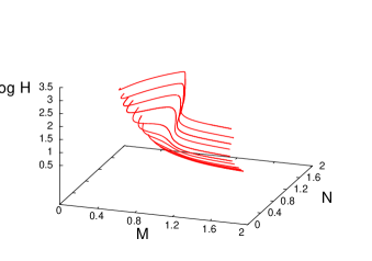
Figure 4: (Color online) AS-AS modes with broken antisymmetry. Panels (a,b) and (c) display, severally, the asymmetries of components $\phi$ and $\psi$, defined as per Eq. (42), and the total energy vs. norms $M$ and $N$ of the two components.

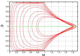
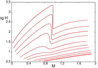
Figure 5: (Color online) The projections of the three-dimensional plots from Fig. 4(a) (left panel) and Fig. 4(c) (right panel) onto the two-dimensional planes of $\left(M,\Delta\Theta_{\phi}\right)$ and $\left(M,\ln H\right)$, respectively.

In connection to the pictures displayed in Figs. 4 and 5, it is relevant to mention that, in the single-component model, the mode with the unbroken antisymmetry exists in an infinite domain limited from below, $1.84<M<\infty$. On the contrary, we here observe that the norms of the “broken” AS-AS solutions take values in a limited domain. As seen in Fig. 5, the corresponding existence plot also contains a lacuna, and, in addition to that, it is confined to values $\left|\Delta\Theta_{\phi}\right|<1$. A formally similar bifurcation in the single-component model, should it be possible, might again seem as a loop detached from the unbroken-antisymmetry modes, which does not reach the limit values of $\left|\Delta\Theta_{\phi,\psi}\right|=1$.

To consider the bifurcation which actually accounts for emergence of the “broken” AS-AS solutions from their counterparts with the exact antisymmetry, it is convenient (as said above) to fix one of the chemical potentials, $\lambda$ or $\mu$, varying the other one. The analysis of the numerical results demonstrates that the antisymmetry-breaking bifurcation occurs, with the variation of $\lambda$, when $|\mu|$ takes values exceeding $\left(|\mu|\right)_{\min}=0.0601$ (indeed, for $|\mu|\rightarrow 0$ one should actually return to the single-component model parameterized by $\lambda$, where the AS mode does not undergo any bifurcation). Emerging from the branch with the unbroken antisymmetry, the solution of the broken AS-AS type eventually merges back into the original branch, as $|\lambda|$ attains a certain maximal value (which increases with the increase of fixed $|\mu|$). If $|\lambda|$ and/or $|\mu|$ remain small enough, the numerical results demonstrate a one-to-one correspondence between the chemical potentials and the corresponding norms, which grow monotonously with the absolute values of the chemical potentials. However, unlike the modes of the Sm-Sm type, for the AS-AS solutions this correspondence breaks down at larger values of $|\lambda|$ and $|\mu|$.

If the fixed chemical potential exceeds another critical value, $\left(|\mu|\right)_{\mathrm{cr}}=0.198$, an additional bifurcation occurs on the broken-AS-AS branch, giving rise to two additional solution families. With the further increase of the absolute value of the varying chemical potential, $|\lambda|$, at some point $|\lambda|=\left(|\lambda|\right)_{\max}$ one of the secondary branches merges with the original one from which it had emerged. The other secondary branch extends to larger values of $|\lambda|$, and eventually merges back into the underlying family of the solutions with the unbroken antisymmetry. The range where the secondary branches are found expands with the increase of fixed $|\mu|$. Another generic feature of the bifurcation, which is responsible for the merger of the broken-AS-AS branch back into its unbroken counterpart, is that this happens when one norm is much larger than the other – typically, at $M\simeq 0.05,$ while $N\simeq 2$.

II.3.3 Solutions obtained from the symmetric-antisymmetric modes (S-AS type)

The existence of modes with unbroken or broken mixed symmetry, of the S-AS type, is another obvious difference of the two-component system from its single-component predecessor. As might be expected, these solutions exist only in the region of the $\left(M,N\right)$ plane where the Sm-Sm and AS-AS states coexist. The global structure of the S-AS family with the broken symmetry and antisymmetry is displayed in Fig. 6 by means of plots showing the asymmetry measures of its initially symmetric ($\phi$) and antisymmetric ($\psi$) components, as well as the total energy, vs. the norms. Since the pattern of the solutions is rather complex, we complement Fig. 6 by Fig. 7, where the projection of the three-dimensional plots of the asymmetry measure of components $\phi$ and $\psi$ from Figs. 6(a),(b) onto the two-dimensional planes of $\left(M,\Delta\Theta_{\phi}\right)$ and $\left(M,\Delta\Theta_{\psi}\right)$, respectively, is presented.

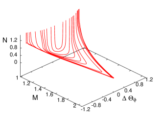
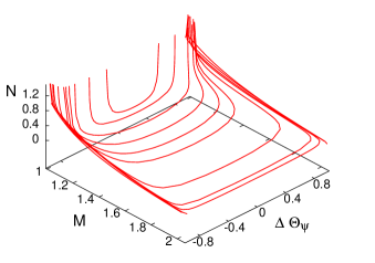
(a)       (b)  (c)

Figure 6: (Color online) The family of mixed-symmetry S-AS modes, with the broken (anti)symmetry. (a) and (b): The asymmetry measures of the symmetric and antisymmetric fields, $\phi$ and $\psi$, respectively. (c) The energy of the S-AS modes with the broken and unbroken (anti)symmetries vs. norms $M$ and $N$.

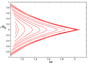
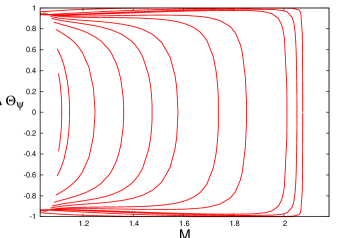
Figure 7: (Color online) Projections of the three-dimensional plots from Fig. 6(a) (left panel) and Fig. 6 (b) (right panel) onto the two-dimensional planes of $\left(M,\Delta\Theta_{\phi}\right)$ and $\left(M,\Delta\Theta_{\psi}\right)$, respectively.

These plots are very different from those for the Sm-Sm and AS-AS modes, cf. Figs. 3-5. To consider the relation between the mixed-symmetry modes with the their Sm-Sm and AS-AS counterparts, it is relevant to stress, that, as may be naturally expected, the branch of S-AS solutions with unbroken (anti)symmetries smoothly merges into the corresponding solutions on the Sm-Sm type in the limit of the vanishing norm $N$ in the AS component. On the other hand, when the latter norm ($N$) increases, the energy of the system increases too, and the configuration smoothly approaches the opposite limit of the AS-AS solution. If chemical potential $|\lambda|$ is large enough, the latter limit corresponds to vanishing norm $M$ of the Sm component. However, for $|\lambda|<0.71$, the $M$-norm does not vanish in the limiting case; instead, it approaches some finite value, whereas the $N$-norm rapidly diverges, as seen in Figs. 6(a) and (b). In fact, this singular behavior is a peculiarity of the model with the $\delta$-functions ($a\rightarrow 0$), while at $a>0$ (in the model with a finite width of the pseudopotential wells) the situation is different, as shown in the next section.

As well as in the cases considered above, the states of the S-AS type with the broken (anti)symmetries emerge from their “unbroken” counterparts through a bifurcation (i.e., they are connected). We discuss this bifurcations in more detail below, considering the model with finite $a$.

It can also be checked, using detailed results of the numerical analysis, that, similar to the case of the Sm-Sm modes, the norms and energy of the S-AS states monotonously grow with the increase of $|\lambda|$ and $|\mu|$, which, in particular, means that the norms are in one-to-one correspondence with the chemical potentials, also similar to the case of the Sm-Sm modes, and in contrast to their AS-AS counterparts. Lastly, comparing Fig. 6(c) to Fig. 3(b), we conclude that, for the same values of norms $M$ and $N$, the energy of the S-AS modes is essentially higher than the energy of the fundamental Sm-Sm states, which suggests that the S-AS states may be more vulnerable to dynamical instabilities.

III The regular model ($a>0$)

III.1 Preliminaries

The results reported in the previous section were based on the numerical solution of coupled cubic equations (35)-(38), which were derived from the analysis of the singular version of the model, with the nonlinear potential represented by the symmetric set of two $\delta$-functions, see Eqs. (9) and (10). It is known from the analysis of the single-component model that this limit case, corresponding to $a\rightarrow 0$ in Eq. (3), is degenerate in several aspects (in particular, the symmetric mode exists only up to a finite value of the norm, see Eq. (43)). In the single-component model, the degeneracy was lifted by the transition to the nonlinearity-modulation function in the general form (3), with finite $a$ (recall that the modulation function keeps its double-well shape up to $a=\sqrt{2}$). Another generic difference of the situation with finite $a$ is that, unlike the case of the nonlinear potential represented by the $\delta$-functions, smooth modulation function (3) may support localized patterns with local maxima shifted from the bottom points, $x=\pm 1$.

We have expanded the analysis of the two-component system to the general case of $g(x)$ taken in the form of (3) with $a>0$. As demonstrated below, the shape of various modes and bifurcations of the respective branches strongly alter, against the limit of $a\rightarrow 0$, starting from values $a\gtrsim 0.1$ (in the single-component model, the essential change in the picture of stationary modes was observed in, roughly, the same range Dong ). All the types of the two-component modes, i.e., Sm-Sm, AS-AS, and S-AS, in their symmetry-broken and unbroken forms alike, feature strong changes against the case of $a\rightarrow 0$ in this region. In fact, these changes are strongly affected by additional modes with broken (anti)symmetry, which appear, at $a$ large enough, still in the single-component model. These modes were not found in Ref. Dong , because they are generated “from nothing” by saddle-node bifurcations, that are disconnected from the symmetry-breaking bifurcation for the symmetric mode, and the stabilization transition for the non-bifurcating antisymmetric one, on which the analysis was focused in Ref. Dong . Therefore, in this section we first present the new results for the single-component model, and then report, in a rather brief form, changes which occur to the compound modes in the two-component system. A full description of the bifurcations in the two-component system with $a\in\left(0,\sqrt{2}\right)$ turns out to be extremely complex, as there is a large number of ramifications of the bifurcation scenarios.

Some comments are relevant too as concerns the numerical methods used for the search of localized solutions to ODE system (7), (8) with $a>0$. In addition to the obvious fact that the numerical analysis had to cover the three-dimensional parameter space, ($a$, $\lambda$, $\mu$), one of difficulties in the numerical study is related to the fact that, for some solutions that had to be obtained, components $u(x)$ and $v(x)$ feature very different (up to a few orders of magnitude) variation rates. Another problem is that, because for small $a$ the coupling between the equations is confined to small neighborhoods of points $x=\pm 1$, it was necessary to use a numerical scheme with a higher density of grid points in those areas.

One numerical method that was used to solve the system of equations (7) and (8) was based on the shooting algorithm Khalil2002 , which is, actually, better suited for producing the solution at smaller values of $a$. Another approach, using the centered-difference-approximation method, turns out to be more appropriate for larger $a$. In particular, the application of the shooting method was assisted by the fact that, for smallest values of $a$, the solution has to be close to that available in the analytical form given by Eqs. (24) and (25) for $a\rightarrow 0$. This fact provided a good initial guess for the shooting method at $a\lesssim 0.4$. An important issue was also the choice of the shooting point. The method did not work with these points taken at $\pm$”infinity”, but it worked well when the point was set in the middle of either nonlinear-potential well (see Eq. (3)). By means of this technique, $5\times 10^{5}$ solutions for the localized modes had been collected, which made it possible to formulate general conclusions about the bifurcation scenarios in the two-component system.

III.2 New results for the single-component model

In Ref. Dong , no bifurcations were found on the branch of single-component antisymmetric modes, both for $a\rightarrow 0$ (where this result was exact) and for finite $a$ (in the numerical form). Our analysis complies with those conclusions. Nevertheless, as shown in Fig. 8, our numerical studies, performed at finite $a$, reveal saddle-node bifurcations (more than a single one, see Fig. 8(c,d)), that generate pairs of single-component modes with broken antisymmetry, which are disjoint from the branch with the unbroken antisymmetry (for this reason, they were not found in Ref. Dong ). An example of the pair of the newly found solutions with the broken antisymmetry is displayed in Fig. 9(a). An essential peculiarity of these modes, which is seen, for instance, in the case of the lower mode displayed in Fig. 9(a), is that they tend to be trapped in a single nonlinear-potential well, instead of being spread between both, which is the case for the mode with the unbroken antisymmetry. It will be shown below that such modes, essentially trapped in a single pseudopotential well, play an essential role in bifurcation scenarios of compound modes of the AS-AS and S-AS types in the two-component system at finite $a$.

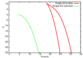
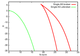
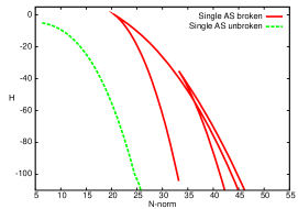
(a)       (b) (c)       (d)

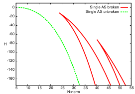
Figure 8: (Color online) Saddle-node bifurcations which generate new pairs of modes with broken antisymmetry in the single-component model (word “single” in the plots stresses this fact) for $a=0.50$ (a), $a=0.60$ (b), $a=0.70$ (c), and $a=0.80$ (d).

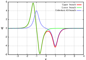
(a) (b)

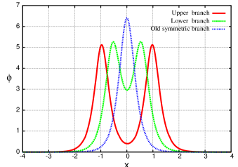
Figure 9: (Color online) (a) A typical example of the pair of single-component modes with broken antisymmetry, which are generated by the saddle-node bifurcation shown in Fig. 8. This example is displayed for $a=0.60$ and chemical potential $|\lambda|=8.0$ of the mode with the unbroken antisymmetry. (b) A typical example of the pair of symmetric single-component double-peak modes which are generated by the saddle-node bifurcation shown in Fig. 10. This example is displayed for $a=0.90$ and chemical potential $|\lambda|=8.0$ of the original mode with the unbroken antisymmetry. “Upper” and “lower” modes, generated by the saddle-node bifurcations, are defined according to the positions of the respective branches in Figs. 8 and 10.

Furthermore, we observe similar saddle-node bifurcations of symmetric and asymmetric solutions in the single-component model. In particular, a pair of new symmetric-solution branches, generated by such a bifurcation, is displayed in Fig. 10. These bifurcations take place on the “old” symmetric and asymmetric branches at some critical values of $a$ (in contrast to the bifurcations displayed in Fig. 8, which are disconnected from the “old” branch of the antisymmetric solutions). For the asymmetric and symmetric solutions, this happens at $a=0.67$ and $a=0.72$, respectively (the bifurcation which gives rise to the pair of the asymmetric branches is not displayed here). As $a$ grows beyond these critical values, the new branches move away from the parent ones. It may happen that more pairs of branches emerge through additional saddle-node bifurcations (cf. Fig. 8, where two such bifurcations are shown for the broken antisymmetric solutions), but we did not aim to look for them.

The difference of the newly emerging symmetric states from the original one, which evolves continuously starting from $a=0$, is that, at relatively large values of $a$, the original mode features a single-peak shape, while the new solutions are shaped as twin-peak modes, see Fig. 9(b).

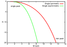
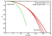
(a)       (b)       (c)

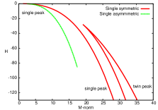
Figure 10: (Color online) The saddle-node bifurcation which generates a new pair of symmetric modes in the single-component model. At $a=0.60$ (prior to the saddle-node bifurcation, panel (a)), only the “old” branch of the symmetric solutions is present. New symmetric branches, generated by the bifurcation, appear as $a\geq 0.72$. The new symmetric branches are plotted, along with the old one, for $a=0.80$ (b), and for $a=0.90$ (c).

III.3 Bifurcations of the symmetric-symmetric (Sm-Sm) branches in the two-component system

To understand the evolution of the Sm-Sm branches at finite $a$ in the two-component system, we select a characteristic value, $a=0.6$. The analysis was performed by fixing chemical potential $\lambda$ which is associated with component $\phi$, and scanning the configuration space of the system by letting vary the other chemical potential, $\mu$, which is associated with component $\psi$. At all values of $\lambda$ and $\mu$, branches of solutions of the Sm-Sm types with unbroken and broken symmetries, have been found, the former ones always having lower energy (6), which suggests that the symmetry breaking may tend to destabilize the modes.

The branch of the Sm-Sm solutions with the broken symmetry smoothly arises from the corresponding single-component asymmetric state, trapped in one of the nonlinear potential wells. In the course of its evolution following the variation of $\mu$, this branch evolves towards the other well, where the other component of the “broken” Sm-Sm solution approaches the respective asymmetric state of the single-component model, while the mate component vanishes.

Similarly, the Sm-Sm branch with the unbroken symmetry arises from the corresponding symmetric solution of the single-component model, at some critical value of $\mu$, and eventually merges into another symmetric state, in which, again, only a single component is present, but the other one. Thus, in both cases of the Sm-Sm modes with broken and unbroken symmetries, the evolution along the branch of the two-component solutions essentially amounts to the conversion of one single-component mode (resp., asymmetric or symmetric) into the mode represented by the originally missing component, while the opposite one vanishes. These bifurcation scenarios for the Sm-Sm branches are illustrated by Fig. 11. They persist in the interval of $0.16<a<0.72$.

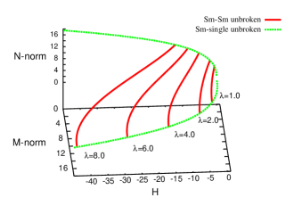
(a) (b)

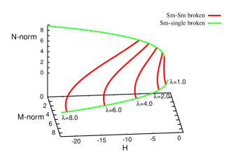
Figure 11: (Color online) The bifurcation scenarios, at $a=0.60$, for the Sm-Sm modes with unbroken (a) and broken (b) symmetries, displayed by means of curves showing the evolution of energy (6) with the variation of chemical potential $\mu$, at the following fixed values of the chemical potential of the other component: $|\lambda|=1.0,2.0,4.0,6.0$ $8.0$.

At $a>0.72$, the system keeps the scenarios described above, but also gives rise to new ones, which involve the additional symmetric modes in the single-component model generated by the saddle-node bifurcation (see Figs. 9(b) and 10). In particular, at $a=0.8$ for fixed $|\lambda|=4.0$, there is a new branch of solutions with the unbroken symmetry, which smoothly arises from the lower symmetric state generated by the saddle-node bifurcation in the single-component model. As shown in Fig. 12(a), this two-component branch makes a loop in the norm space, $\left(M,N\right)$, and then merges into the upper symmetric state of the single-component model, which is generated by the above-mentioned saddle-node bifurcation. In this case, the second component of the Sm-Sm system vanishes at both ends of the branch. For larger absolute values of the chemical potential, say $|\lambda|=8.0$, a different behavior is observed. Instead of coming back to the upper state of the single-component model generated by the saddle-node bifurcation, the first component vanishes, while the other one evolves towards the corresponding upper-state solution of the single-component model, as shown in Fig. 12(b).

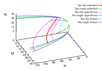
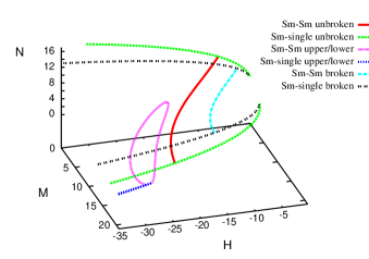
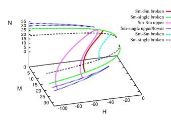
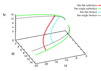
(a)       (b)       (c)       (d)       (e)       (f)

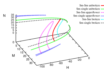
Figure 12: (Color online) The same as Fig. 11,  but for $|\lambda|=4.0$ and $|\lambda|=8.0$ (left and right columns), for $a=0.8$, $0.9$, and $1.0$ (the first, second, and third rows, respectively).

As $a$ increases further, $|\lambda|$ must be very large to support a link between the first and second components playing the role of the end states of the Sm-Sm branch. For $a=0.9$, for example, both at $|\lambda|=4.0$ and $|\lambda|=8.0$, the Sm-Sm branch makes a loop in the norm space, emerging from the lower-state solution of the single-component model with the second component being absent. This branch evolves towards the upper-state symmetric solution of the single-component model with the second component vanishing again, as shown in Figs. 12 (c,d). The further increase of $a$ at relatively small values of $|\lambda|$ eliminates the looped branch; however, the branches of the two-component solutions with the broken and unbroken symmetries, which link the corresponding single-component modes (asymmetric or symmetric, respectively) still persist, as shown in Fig. 12(e). Nevertheless, at larger values of $\lambda$ the analysis reproduces the same pattern as observed before, cf. Figs.  12(d) and 12(f).

III.4 Bifurcations of the antisymmetric-antisymmetric (AS-AS) branches

The structure of the configuration space of the AS-AS solutions in the model with finite $a$ is complex. It can also be studied by fixing, say, $a=0.6$ and one of the chemical potentials ($\lambda$, which is associated with the $\phi$-component), and scanning the space by varying $\mu$, which is associated with component $\psi$. In fact, the picture displayed below for $a=0.6$ adequately represents the situation in the interval of $0.16<a<0.76.$

Similar to the case of the Sm-Sm modes considered above, the description of various bifurcation scenarios for the AS-AS branches, with the broken and unbroken antisymmetry alike, essentially reduces to identifying pairs of states of the single-component models which are linked by these branches. First, at relatively small fixed values of $|\lambda|$ (see Figs. 13(a,b)), we observe a branch of the AS-AS solutions with broken antisymmetry, which arises smoothly from the “unbroken” AS-AS family, at some critical value of $\mu$. The asymmetry of the states rapidly increases along this branch.

The branch extends up to a second critical value of $\mu$, where it merges back into the “unbroken” AS-AS branch. Shortly afterwards, the unbroken branch itself merges into the corresponding solution of the single-component model. This scenario implies that, typically, one of the components, e.g., $\phi$, gradually approaches the limit solution with the unbroken antisymmetry, while the other component remains strongly asymmetric almost until the end of the branch, where its asymmetry abruptly drops to zero.

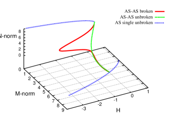
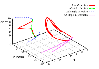
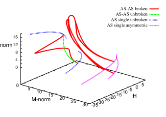
(a)       (b)       (c)       (d)

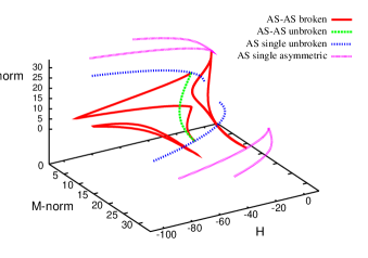
Figure 13: (Color online) The picture of the bifurcation scenarios similar to that in Fig. 11, but for AS-AS branches with $a=0.6$ and$\leavevmode\nobreak\ \lambda=1.0\leavevmode\nobreak\$(a), $1.5\leavevmode\nobreak\$(b), $4.0\leavevmode\nobreak\$(c), and $8.0$ (d).

As $|\lambda|$ increases beyond a critical value, the above-mentioned broken-antisymmetry modes, generated by the saddle-node bifurcations in the single-component model, come into the play, making the evolution of the AS-AS branches quite involved. A new branch arises smoothly from the new broken-antisymmetry solution of the single-component model, which is trapped in one of the nonlinear potential wells. Fixing $|\lambda|=1.5$ and varying $\mu$, we observe that this branch first makes a double loop in the norm space, $\left(M,N\right)$, with both components remaining trapped in the potential well, as shown in Figs.  13(c,d). Surprisingly, almost immediately another branch arises. The evolution along the new branch amounts to a transition of one of the components from one nonlinear-potential well to the other. One of the components on this branch looks like an S-AS bound state, rather than a single AS state, as shown in Fig. 14(b).

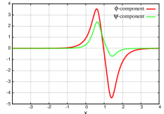
(a) (b)

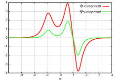
Figure 14: (Color online) (a) and (b): Examples of AS-AS solutions belonging, respectively, to the lower (closed loop) and upper (transition) branches in Fig. 13(c), with $a=0.6$, $\mu=8.0$ and $|\lambda|=4.0$.

To consider in further detail how the evolution of the AS-AS branches depends on the value of $a$, we now fix chemical potential $\lambda$ and consider a range of values of $a$. In the case of not very large $|\lambda|$, the AS-AS branch with the broken antisymmetry again originates from the “unbroken” AS-AS branch, as $\mu$ increases above some critical value. Since this branch is actually observed in the entire parameter space, including the limit case with the $\delta$-functions ($a\rightarrow 0$), it may be naturally called the fundamental AS-AS branch with the broken antisymmetry. Along this branch, one of the components, say $\phi$, rapidly grows with the increase of $|\mu|$, remaining localized in one nonlinear-potential well [as seen in Fig. 15(a)], while the other component, $\psi$, has two well-pronounced peaks near $x=\pm 1$. The evolution along this branch proceeds through the decrease of the maximum values of the second component, so that, at some point, the mode approaches the limit case of two AS states localized around opposite minima of the nonlinear potential, see Fig. 15(b). Finally, the system evolves towards the mirror image of the initial configuration, where the $\phi$ component features maxima near $x=\pm 1$, while component $\psi$ is trapped in the nonlinear potential well opposite to that where $\phi$ was originally trapped, see Fig. 15(c). As $\mu$ approaches the second critical value, the branch merges back into the AS-AS state with the unbroken antisymmetry. Actually, this branch links two single-component AS solutions with the unbroken antisymmetry.

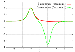
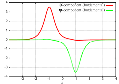
(a) (b) (c)

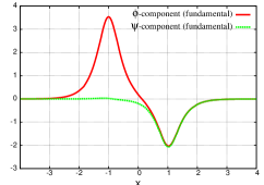
Figure 15: (Color online) Examples of AS-AS solutions with the broken antisymmetry at three points of the fundamental branch with $a=0.8$, $|\mu|=4.0$ and $|\lambda|=4.0$.

The evolution pattern becomes still more complex at larger values of $|\lambda|$. In that case (for instance, at $|\lambda|=4$) , the building blocks of the AS-AS states are again single-component AS modes with the strongly broken antisymmetry, each localized around one minimum of the nonlinear potential. The evolution trajectory in the configuration space may then feature two loops. Along the first one, the system moves from the localization in one nonlinear potential well to the other, simultaneously swapping the two components (the one which was originally dominating and its initially vanishing counterpart). Continuing the evolution along the second loop, the system swaps the two components once again (not shown here in detail).

III.5 Bifurcations of the symmetric-antisymmetric (S-AS) branches

The evolution of branches of the S-AS type in the system with finite $a$ also strongly differs from what was presented above for the system with the set of the $\delta$-functions, corresponding to $a\rightarrow 0$. As well as the solutions of the Sm-Sm and AS-AS types, in the present case the evolution also amounts, essentially, to the switch between different states of the single-component model, linked by the branch of the S-AS type, with the unbroken or broken (anti)symmetries. To present the results, we again start with $a=0.6$, fixing the chemical potentials ($\mu$) which is associated with the symmetric component ($\phi$), and scan the configuration space by varying the chemical potential ($\lambda$) associated with the antisymmetric component, $\psi$.

Following the general pattern outlined above for other species of the two-component solutions, the “broken” S-AS branch arises from its counterpart with the unbroken (anti)symmetries, at some critical value of $\lambda$. The energy of the emerging “broken” branch rapidly grows with $|\lambda|$, as seen in Fig.  16.

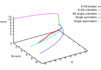
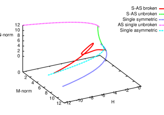
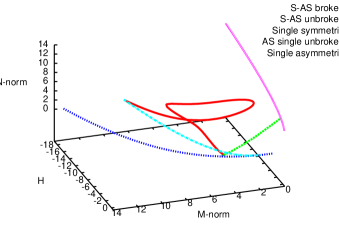
(a)       (b)       (c)       (d)

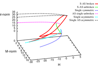
Figure 16: (Color online) Branches of modes of the S-AS type: the evolution of the energy (6) in the norm space, $\left(M,N\right)$, at $a=0.6$ and $|\mu|=0.2\leavevmode\nobreak\$(a), $|\mu|=0.5\leavevmode\nobreak\$(b), $|\mu|=1.0\leavevmode\nobreak\$(c), and $|\mu|=1.5$ (d).

The emergence and evolution of these S-AS branches is further illustrated by Fig. 17, which displays the pattern of the modes at $|\mu|=1.5,1.0,0.5,0.2$. We observe that, if $|\mu|$ remains relatively small, the increase of $|\lambda|$ leads to a bifurcation between the “broken” and “unbroken” S-AS modes. As $|\lambda|$ slightly decreases below this critical value, the norm of the AS component in the “unbroken” S-AS mode rapidly drops to zero, so that the branch almost immediately merges into the branch of symmetric solutions of the single-component model. As $|\lambda|$ increases above the critical value, the “broken” S-AS branch evolves towards the limit of a single-component “broken” AS solution which is strongly localized in one well of the nonlinear potential, while the “unbroken” S-AS branch approaches the “unbroken” AS mode of the single-component model.

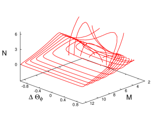
(a)       (b)

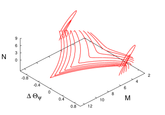
Figure 17: S-AS branches in the system with $a=0.60$: the evolution of the asymmetry of the (originally) symmetric field $\phi$ (a) and antisymmetric field $\psi$ (b) in the norm space, $\left(M,N\right)$.

Another look at the evolution of the S-AS branches is suggested by the general circumstance, similar to that emphasized above, in the course of the analysis of the solution families of the Sm-Sm and AS-AS types, viz., that various branches of two-component solutions may be realized as links connecting the basic modes of the three types: the two-component ones with the unbroken (anti)symmetry, single-component symmetric/antisymmetric/asymmetric states, and the other above-mentioned species of single-component solutions, which are almost entirely localized in one well of the nonlinear potential. Below, we refer to these three basic types of the modes as A, B, and C, respectively. In particular, the picture of the evolution of the “broken” S-AS branches, as described above, may be interpreted so that the broken-(anti)symmetry branch evolves from state A towards B. For example, at small values of $|\mu|$, the “broken” S-AS states are weakly localized, and the increase of $|\lambda|$ drives the system towards state B without bifurcations. At $|\mu|>0.15$, the asymmetry of the AS component changes its sign, but there is still no bifurcation, with energy (6) monotonically depending on norms $M$ and $N$.

At $|\mu|>0.37$, there emerges the above-mentioned single-component mode (C), strongly localized in one well of the nonlinear potential, with a result that the AS state tends to be trapped near this mode, before it will be driven to mode B. This circumstance changes results of the bifurcation, as can be observed in terms of the asymmetries and energy in Figs. 17 and 19(a). Another interpretation is that there is an additional state which appears at the bifurcation point, built as a combination of a symmetric mode in one component and a new AS mode with broken antisymmetry, see Fig  19. This means that three branches are observed in this region, with the evolving one attracted to state C and oscillating about it for a while, before plunging to the limit of the vanishing AS component (state B).

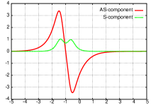
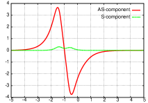
(a)       (b)       (c)

Figure 18: (Color online) The evolution of modes of the S-AS type with the broken antisymmetry, approaching the effectively single-component mode (C, as defined in the text). In terms of Fig. 8, C is the upper AS state with the broken antisymmetry, generated by the saddle-node bifurcation and trapped in one nonlinear potential well. The parameters are $a=0.6$, $|\mu|=1.5$, and $|\lambda|=6.5$ (a), $7.40\leavevmode\nobreak\$(b) and $\lambda=7.43$ (c), respectively.

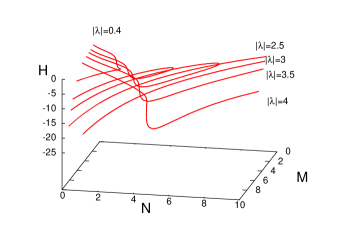
(a)       (b)

Figure 19: (Color online) (a) The energy of the S-AS states with the broken (anti)symmetry at $a=0.6$ and $|\lambda|=4.0,3.5,3.0,2.5,2.0,1.0,0.7,0.4$, in the $\left({M,N}\right)$ plane. (b) Profiles of the two components of the new S-AS solution found in a vicinity of state C (defined in the text), at $a=0.6$, and $|\mu|=4.00,$ $|\lambda|=0.791$.

The picture of the evolution of the S-AS branches outlined above is valid in the interval of $0.1<a<0.67$. Additional ramifications of the picture, which are not presented here, are revealed by the analysis at larger values of $a$.

IV Conclusions

In this work, we have introduced the two-component one-dimensional model with the nonlinear (pseudo)potential represented by two strongly localized potential wells. The subject of the analysis is the evolution of various two-component modes of the three types: Sm-Sm (symmetric-symmetric), AS-AS (antisymmetric-antisymmetric), and S-AS (mixed states with symmetric and antisymmetric components), and the related SSB (spontaneous-symmetry-breaking) effects. In the limit of the nonlinearity modulation represented by the set of two $\delta$-functions, the solution was obtained in the semi-analytical form. The consideration of this solution demonstrates new features of the two-component modes with spontaneously broken (anti)symmetries, which are qualitatively different from what was previously reported in the single-component model. In particular, the spontaneous breaking of the antisymmetry is possible only in the two-component system, and, obviously, S-AS states, with the unbroken or broken mixed symmetry exist only in the two-component system.

In the model based on the set of two nonlinear potential wells of a finite width, the evolution and bifurcation scenarios were found to be still more complex. First, new results for the case of finite potential wells were reported for the single-component model. These are pairs of modes with the broken antisymmetry, and pairs of twin-peak symmetric modes, generated by isolated saddle-node bifurcations, in either case. Then, numerous complex scenarios of the evolution of the Sm-Sm, AS-AS, and S-AS branches with the broken (anti)symmetries may be interpreted in terms of routes linking three species of basic modes: two-component states with the unbroken (anti)symmetries, “unbroken” or “broken” single-component states featuring density peaks in both nonlinear-potential wells, and, finally, single-component states effectively trapped in a single well.

It remains to systematically analyze the stability of diverse two-component stationary modes reported in this work. Challenging problems may also be to extend the model to a set of several nonlinear spots, including a periodic lattice, and, on the other hand, to develop the two-dimensional (2D) version of the two-component system, following the recent analyses of the 2D extensions of the single-component model Hung ; new .

References

- (1) D. Landau, E. M. Lifshitz, Quantum Mechanics (Moscow: Nauka Publishers, 1974).
- (2) S. Giorgini, L. P. Pitaevskii, S. Stringari, Rev. Mod. Phys. 80 (2008) 1215; H. T. C. Stoof, K. B. Gubbels, D. B. M. Dickrsheid, Ultracold Quantum Fields (Springer: Dordrecht, 2009).
- (3) Y. S. Kivshar G. P. Agrawal, Optical Solitons: From Fibers to Photonic Crystals (Academic Press: San Diego).
- (4) E. A. Ostrovskaya, Y. S. Kivshar, M. Lisak, B. Hall, F. Cattani, D. Anderson, Phys. Rev. A 61 (2000 031601); R. D’Agosta, B. A. Malomed, C. Presilla, Phys. Lett. A 275 (2000) 424; R. K. Jackson M. I. Weinstein, J. Stat. Phys. 116 (2004) 881; D. Ananikian T. Bergeman, Phys. Rev. A 73 (2006) 013604; E. W. Kirr, P. G. Kevrekidis, E. Shlizerman, M. I. Weinstein, SIAM J. Math. Anal. 40 (2008) 566.
- (5) G. J. Milburn, J. Corney, E. M. Wright, D. F. Walls, Phys. Rev. A 55 (1997) 4318; A. Smerzi, S. Fantoni, S. Giovanazzi, S. R. Shenoy, Phys. Rev. Lett. 79 (1997) 4950; S. Raghavan, A. Smerzi, S. Fantoni, S. R. Shenoy, Phys. Rev. A 59 (1999) 620; K. W. Mahmud, H. Perry, W. P. Reinhardt, Phys. Rev. A 71 (2005) 023615; E. Infeld, P. Ziń, J. Gocalek, M. Trippenbach, Phys. Rev. E 74 (2006) 026610; G. Theocharis, P. G. Kevrekidis, D. J. Frantzeskakis, P. Schmelcher, Phys. Rev. E 74 (2006) 056608; G. L. Alfimov D. A. Zezyulin, Nonlinearity 20 (2007) 2075; C. Wang, P. G. Kevrekidis, N. Whitaker, B. A. Malomed, Physica D 237 (2008) 2922.
- (6) M. Albiez, R. Gati, J. Fölling, S. Hunsmann, M. Cristiani, M. K. Oberthaler, Phys. Rev. Lett. 95, (2005) 010402); R. Gati, M. Albiez, J. Fölling, B. Hemmerling, M. K. Oberthaler, Appl. Phys. B 82 (2006) 207.
- (7) P. G. Kevrekidis, Z. Chen, B. A. Malomed, D. J. Frantzeskakis, M. I. Weinstein, Phys. Lett. A 340 (2005) 275.
- (8) J. C. Eilbeck, P. S. Lomdahl, A. C. Scott, Physica D 16 (1985) 318.
- (9) A. W. Snyder, D. J. Mitchell, L. Poladian, D. R. Rowland, Y. Chen, J. Opt. Soc. Am. B 8 (1991) 2101.
- (10) C. Paré, M. Fłorjańczyk, Phys. Rev. A 41 (1990) 6287; A. I. Maimistov, Kvant. Elektron. 18 (1991) 758 [Sov. J. Quantum Electron. 21 (1991) 687]; N. Akhmediev A. Ankiewicz, Phys. Rev. Lett. 70 (1993) 2395; P. L. Chu, B. A. Malomed, G. D. Peng, J. Opt. Soc. A B 10 (1993) 1379; B. A. Malomed, in: Progr. Optics 43, 71 (E. Wolf, editor: North Holland, Amsterdam, 2002).
- (11) W. C. K. Mak, B. A. Malomed, P. L. Chu, J. Opt. Soc. Am. B 15 (1998) 1685.
- (12) A. Gubeskys B. A. Malomed, Phys. Rev. A 75 (2007) 063602.
- (13) M. Matuszewski, B. A. Malomed, M. Trippenbach, Phys. Rev. A 75 (2007) 063621.
- (14) M. Trippenbach, E. Infeld, J. Gocalek, M. Matuszewski, M. Oberthaler, B. A. Malomed, Phys. Rev. A 78 (2008) 013603.
- (15) L. Salasnich, B. A. Malomed, F. Toigo, Phys. Rev. A 81 (2010) 045603.
- (16) G. Iooss D. D. Joseph, Elementary Stability Bifurcation Theory (Springer-Verlag: New York, 1980).
- (17) W. A. Harrison, Pseudopotentials in the Theory of Metals (Benjamin: New York, 1966).
- (18) L. C. Qian, M. L. Wall, S. Zhang, Z. Zhou, H. Pu, Phys. Rev. A 77 (2008) 013611.
- (19) Y. V. Kartashov, B. A. Malomed, L. Torner, Solitons in nonlinear lattices, Rev. Mod. Phys. Rev. Mod. Phys. 83 (2011) 247.
- (20) T. Mayteevarunyoo, B. A. Malomed, G. Dong, Phys. Rev. A 78 (2008) 053601.
- (21) N. Dror, B. A. Malomed, Solitons supported by localized nonlinearities in periodic media, Phys. Rev. A 83 (2011) 033828.
- (22) B. A. Malomed, M. Ya. Azbel, Phys. Rev. B 47 (1993) 10402.
- (23) P. O. Fedichev, Y. Kagan, G. V. Shlyapnikov, J. T. M. Walraven, Phys. Rev. Lett. 77 (1996), 2913; M. Theis, G. Thalhammer, K. Winkler, M. Hellwig, G. Ruff, R. Grimm, J. H. Denschlag, ibid. 93 (2004) 123001.
- (24) J. Hukriede, D. Runde, D. Kip, J. Phys. D: Appl. Phys. 36 (2003) R1.
- (25) N. V. Hung, P. Ziń, M. Trippenbach, B. A. Malomed, Phys. Rev. E 82 (2010) 046602.
- (26) T. Mayteevarunyoo, B. A. Malomed, A. Reoksabutr, “Spontaneous symmetry breaking of photonic and matter waves in two-dimensional pseudopotentials”, J. Mod. Opt., in press.
- (27) G. Herring, P. G. Kevrekidis, B. A. Malomed, R. Carretero-González, D. J. Frantzeskakis Phys. Rev. E 76 (2007) 066606.
- (28) Lj. Hadžievski, G. Gligorić, A. Maluckov, B. A. Malomed, Phys. Rev. A 82 (2010) 033806.
- (29) M. I. Molina G. Tsironis, Phys. Rev. B 47, 15330 (1993); B. C. Gupta K. Kundu, ibid. 55 (1997) 894; 55 (1997) 11033.
- (30) V. A. Brazhnyi B. A. Malomed, Phys. Rev. A 83 (2011) 053844.
- (31) E. Bulgakov, K. Pichugin, A. Sadreev, Phys. Rev. B 83 (2011) 045109.
- (32) S. Ashhab C. Lobo, Phys. Rev. A 66 (2002) 013609; B. Xia, W. Hai, G. Chong, Phys. Lett. A 351 (2006) 136; X. Xu, L. Lu, Y. Li, Phys. Rev. A 78 (2008) 043609; C. Wang, P. G. Kevrekidis, N. Whitaker, B. A. Malomed, Physica D 327 (2008) 2922; I. I. Satija, P. Naudus, R. Balakrishnan, J. Heward, M. Edwards, C. W. Clark, Phys. Rev. A 79 (2009) 033616; B. Julia-Diaz, M. Guilleumas, M. Lewenstein, A. Polls, A. Sanpera, ibid. 80 (2009) 023616; B. Julia-Diaz, M. Mele-Messeguer, M. Guilleumas, A. Polls, ibid. 80 (2009) 043622; M. Tujillo-Martinez, A. Posazhennikova, J. Kroha, Phys. Rev. Lett. 103 (2009) 105302; G. Mazzarella, M. Moratti, L. Salasnich, M. Salerno, F. Toigo, J. Phys. B: At. Mol. Opt. Phys. 42 (2009) 125301; G. Mazzarella, M. Moratti, L. Salasnich, F. Toigo, ibid. 43 (2010) 065303; M. Yasunaga M. Tsubota, J. Low Temp. Phys. 158 (2010) 51; G. Mazzarella, B. Malomed, L. Salasnich, M. Salerno, F. Toigo, J. Phys. B: At. Mol. Opt. Phys. 44 (2011) 035301.
- (33) T. Zibold, E. Nicklas, C. Gross, M. K. Oberthaler, Phys. Rev. Lett. 105 (2010) 204101.
- (34) A. Shapira, N. Voloch-Bloch, B. A. Malomed, A. Arie, J. Opt. Soc. Am. B 28 (2011) 1481.
- (35) M. Vakhitov A. Kolokolov, Radiophys. Quantum Electron. 16 (1973) 783.
- (36) L. Bergé, Phys. Rep. 303 (1998) 259.
- (37) K. Li, P. G. Kevrekidis, B. A. Malomed, and D. J. Frantzeskakis, Phys. Rev. E 84 (2011) 056609.
- (38) H. K. Khalil, Nonlinear systems (Third Edition), Prentice Hall, 2002.