The Optical Depth of Hii regions in the Magellanic Clouds

Abstract

-THIS ELECTRONIC VERSION INCLUDES TABLES 5 AND 6 AS REVISED IN THE ERRATUM-
- THE ERRATUM HAS BEEN BUNDLED AS A SEPARATE FILE IN THIS ARXIV SUBMISSION -
We exploit ionization-parameter mapping as a powerful tool to measure the optical depth of star-forming Hii regions. Our simulations using the photoionization code Cloudy and our new, SurfBright surface brightness simulator demonstrate that this technique can directly diagnose most density-bounded, optically thin nebulae using spatially resolved emission line data. We apply this method to the Large and Small Magellanic Clouds, using the data from the Magellanic Clouds Emission Line Survey. We generate new Hii region catalogs based on photoionization criteria set by the observed ionization structure in the [S$\rm II$]/[O$\rm III$] ratio and H$\alpha$ surface brightness. The luminosity functions from these catalogs generally agree with those from H$\alpha$-only surveys. We then use ionization-parameter mapping to crudely classify all the nebulae into optically thick vs optically thin categories, yielding fundamental new insights into Lyman continuum radiation transfer. We find that in both galaxies, the frequency of optically thin objects correlates with H$\alpha$ luminosity, and that the numbers of these objects dominate above $\log\mbox{$L$}/({\rm erg\ s^{-1}})\geq 37.0$. The frequencies of optically thin objects are 40% and 33% in the LMC and SMC, respectively. Similarly, the frequency of optically thick regions correlates with Hi column density, with optically thin objects dominating at the lowest $N{\rm(HI)}$. The integrated escape luminosity of ionizing radiation is dominated by the largest regions, and corresponds to luminosity-weighted, ionizing escape fractions from the Hii region population of $\geq 0.42$ and $\geq$ 0.40 in the LMC and SMC, respectively. These values correspond to global galactic escape fractions of 4% and 11%, respectively. This is sufficient to power the ionization rate of the observed diffuse ionized gas in both galaxies. Since our optical depth estimates tend to be underestimates, and also omit the contribution from field stars without nebulae, our results suggest the possibility of significant galactic escape fractions of Lyman continuum radiation.
-THIS ELECTRONIC VERSION INCLUDES TABLES 5 AND 6 AS REVISED IN THE ERRATUM-

1. Introduction

Few of the rich and complex disciplines in astrophysics affect our understanding of the Universe as deeply as the diffusion of ionizing radiation from stars and its interaction with surrounding matter. Of all the known sinks and sources of energy, the ionizing radiation released by O stars during their short lives has great consequences by 1) determining the structure and energy balance of the interstellar medium (ISM) in galaxies, 2) generating diagnostics of stellar populations and interstellar conditions, and 3) providing an important source of the Lyman continuum radiation field during cosmic reionization.

The luminosity and spectral energy distribution (SED) of massive stars make them a powerful source of ionizing radiation within star forming galaxies (e.g., Abbott, 1982; Reynolds, 1984). Their power has been demonstrated by studies of nearby galaxies which show that the Lyman-continuum (LyC) radiation from O-stars embedded within Hii regions, combined with those in the field, is luminous enough to balance the incessant recombination and cooling of the diffuse, warm ionized medium (WIM) in galaxies (e.g., Oey & Kennicutt 1997; Hoopes & Walterbos 2000; Oey et al. 2004; for a recent review of the WIM see Haffner et al. 2009). Radiative transfer calculations also demonstrate that injecting ionizing radiation from stars into the WIM not only heats the gas, but also acts to decrease its cooling efficiency (Cantalupo, 2010), preventing the catastrophic cooling of warm diffuse gas which would lead to unregulated star formation (e.g. Parravano, 1988; Ostriker et al., 2010). In these ways, ionizing stellar radiation can strongly influence both the ISM structure and star formation rates of galaxies.

The H Balmer recombination lines form beacons of star formation across the universe (e.g., Cowie & Hu 1998). When ionizing photons are all absorbed by gas, H recombination lines are an accurate diagnostic of $Q{\rm(H^{0})}$, the rate at which H ionizing radiation is produced by stars. Multiwavelength emission-line observations and theoretical stellar SEDs are routinely used with observed recombination rates to infer the stellar populations of distant galaxies (e.g., Sullivan et al., 2004; Iglesias-Páramo et al., 2004).

Ionizing radiation from stars may ultimately escape into the intergalactic medium (IGM) before being absorbed. This radiation may be an important source of the cosmic background UV field during the epoch of reionization, some time between redshift $z\sim 11$ (Komatsu et al., 2011) and $z\sim 6$ (Fan et al., 2002). During this time, star-forming galaxies are believed to contribute 10-20% of their total ionizing radiation budget to sustain reionization, because the UV and X-ray field from AGN alone was likely insufficient (Sokasian et al., 2003). Recent detections of faint Ly$\alpha$ emitting galaxies by Dressler et al. (2011) support this view with evidence that aggregate LyC radiation from faint galaxies during this epoch is sufficient to sustain cosmic reionization.

Understanding the radiative transfer of LyC photons from massive stars is therefore a fundamental problem, and although they are well understood in general terms, Hii regions still present a computational challenge because of their greatly varying densities, small-scale structure, and irregular nature. Consequently, Paardekooper et al. (2011) identified radiative transfer of individual nebulae as the main bottleneck which limits our ability to determine the escape fraction of ionizing radiation from star forming galaxies in cosmological simulations. It is thus imperative to understand radiation transport within Hii regions if we are to understand fundamental properties of the universe.

There has been a variety of approaches to evaluate the optical depth of Hii regions. The most direct method compares the ionization rate derived from H$\alpha$ luminosities $L$ to that predicted from the observed ionizing stellar population. Using this approach, Oey & Kennicutt (1997) found that up to half of all ionizing photons generated by stars escape Hii regions to ionize the WIM, also known as diffuse ionized gas (DIG). However, theoretical predictions for the LyC photon emission rate $Q{\rm(H^{0})}$ have decreased significantly (e.g., Martins et al. 2005; Smith et al. 2002), and are now generally consistent with the observed Hii region luminosities (e.g., Voges et al. 2008; Zastrow et al. 2011a). Clearly, until the ionizing fluxes and SEDs of massive stars are definitively established, comparing predicted and observed $L$ will be subject to large systematic uncertainties. Identifying all the ionizing stars is also difficult in regions with significant extinction and crowding.

Other studies attempt to evaluate nebular optical depth by modeling nebular emission lines from ions with different ionization potentials averaged over the entire Hii region (e.g., Relaño et al. 2002; Iglesias-Páramo & Muñoz-Tuñón 2002; Giammanco et al. 2004; Kehrig et al. 2011). However, inhomogeneous, optically-thin nebulae may contain many optically-thick cloudlets. Since the emission-line volume-emissivity is proportional to the square of the electron density, the resulting spatially integrated spectra can be dominated by these dense clumps and resemble the spectrum of an optically-thick, homogeneous nebula, despite small clump-covering-factors (Giammanco et al., 2004). Typically, these studies do not resolve the spatial structure of the emitting gas. Observations either integrate all the nebular light and lose all spatial information, or study structure from a single long slit spectrum. By simplifying the line fluxes of an entire Hii region to a single value, valuable information about the true structure of the gas is lost.

The correlation between DIG surface brightness and proximity to Hii regions is another key piece of evidence for the leakage of ionizing radiation from discrete Hii regions, and can be used to estimate the optical depth. Seon (2009) used these correlations to test a model of M51 where leaking Hii regions explain the observed DIG and H$\alpha$ surface brightness distributions, similar to the method used by Zurita et al. (2002) in NGC 157. However, Seon (2009) found that this model requires a highly rarefied or porous ISM with an anomalously low dust abundance. These details are inconsistent with the known properties of M51, suggesting the models do not fully explain the propagation of radiation in real galaxies.

Thus, existing methods to determine nebular optical depth are subject to large uncertainties; clearly it would be preferable to have a diagnostic that is reliable, effective and simple. Here, we offer such a diagnostic, using an approach that makes it possible to accurately characterize the optical depth of individual Hii regions in the nearest galaxies. In §2, we describe our method; in §3, we apply our technique to the Magellanic Clouds, and use it to generate a new, physically motivated Hii region catalog; and we evaluate our technique in §4. Our results yield powerful new insights on the radiative transfer of LyC radiation from massive stars in these galaxies, which we present in §5.

2. Ionization-Parameter Mapping

With the recent availability of wide-field, narrow-band imaging and tunable filters, the potential of spatially resolved, emission-line diagnostics as constraints on nebular models is being more fully realized, and these techniques can now be applied to entire populations of extragalactic nebulae. We revisit a largely overlooked approach, ionization-parameter mapping (IPM), which is capable of directly assessing the optical depth of ionizing radiation in individual Hii regions (e.g., Koeppen 1979). The technique is based on emission-line ratio mapping, which has been previously employed (e.g., Heydari-Malayeri 1981; Pogge 1988a, b); here, we present a modern development, demonstration, and application. The current approach is driven by newly available data with unprecedented sensitivity, resolution, and spatial completeness. We leverage this data against recent developments in the ability to predict spatially resolved, emission line diagnostics with photoionization models. Our method thus balances the quantitative diagnostics of spectroscopy and the spatial coverage of imaging, yielding a powerful method that is both observationally efficient and straightforward enough to be applied to entire galaxies.

2.1. Evaluating nebular optical depth

For classic, optically-thick Hii regions, there is a transition zone between the central, highly excited region and the neutral environment. These transition zones are characterized by a strong decrease in the excitation, and hence also in the gas ionization parameter, which traces the degree of ionization and photon-to-gas density. Figure 1$a$ and 1$b$ show the radial ionic structure of Strömgren spheres generated by a 38,000 K and 43,000 K star, respectively. These demonstrate the transition from highly ionized inner zones dominated by ${\rm O^{2+}}$ and ${\rm S^{2+}}$ to outer envelopes dominated by ${\rm O^{+}}$ and ${\rm S^{+}}$. The low-ionization transition zone is thicker than the narrow H⁰/H⁺ ionization front where the [S$\rm II$] volume emissivity peaks (Osterbrock & Ferland, 2006); this results from the sensitivity of the [S$\rm II$]/[O$\rm III$] ratio to the radial difference between the ${\rm O^{2+}}$ and $\rm H^{+}$ recombination fronts, which are in turn determined by the LyC optical depth $\tau_{\rm LyC}$ and stellar effective temperature $T_{\rm eff}$. This large scale gradient is a key feature to the application of ionization parameter mapping at great distances. For the models in Figure 1, the assumed ionizing SED is a single WM-Basic stellar atmosphere (Smith et al., 2002) defined by a variable $T_{\rm eff}$ and fixed $Q{\rm(H^{0})}=10^{49}\rm s^{-1}$, equivalent to one O6 V star. Calculations were performed using the Cloudy photoionization code, version C08.00 (Ferland et al., 1998), adopting gas-phase abundances equal to those of the 30 Doradus star-forming region, having log(O/H) = $-3.75$ (Pellegrini et al., 2011). Our models include dust with a gas-to-dust ratio of $\mbox{$A_{\rm V}$}/N{\rm(H)}=1.8\times 10^{-23}~{}{\rm cm^{-2}}$, which is consistent with the ionized gas studied by Pellegrini et al. (2011). We use dust with an LMC size-distribution described by Weingartner & Draine (2001), although our results are not sensitive to the dust abundance. The initial H density $n{\rm{}_{H}}$ is equal to $10~{}{\rm cm^{-3}}$, and the distance $r_{0}=0.1~{}{\rm pc}$ between the illuminated face of the cloud and the ionizing source. Deeper in the cloud $n_{\rm H}$ is set by a hydrostatic equation of state with no magnetic field (${\bf B}=0$ G) described in Pellegrini et al. (2007).

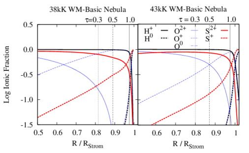
Figure 1.— The radial ionization structure for Strömgren sphere Hii regions photoionized by a $T_{\rm eff}=38$ kK star (left panel) and a 43 kK star (right panel), assuming a gas density of $10\ {\rm cm^{-3}}$. The logarithmic ionization fractions of H⁺(solid, thick black line), H⁰ (dashed, thick black line), O²⁺ (solid, thin blue line), O⁺ (dashed, thin blue line), O⁰ (dash-dot, blue line), S²⁺ (solid, thick red line), and S⁺ (thick, dashed red line) are plotted. The vertical lines mark radii where $\tau_{\rm LyC}$= 0.3 (dotted), 0.5 (dashed) to 1.0 (solid).

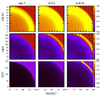
Figure 2.— Models of the observed [S$\rm II$]/[O$\rm III$] surface brightness ratios for nebulae ionized by O3 V, O6 V, and O9.5 V stars, at optical depths $\tau_{\rm LyC}$ of 0.5, 1.0, and 10. A uniform background is assumed, and the units on both axes are in arcsec, projecting the objects at the LMC distance.

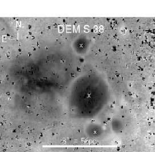
Figure 3.— A map of the [S$\rm II$]/[O$\rm III$] ratio centered on HII region DEM S38. The central region is a classic example of an optically thick nebula with highly ionized gas (low [S$\rm II$]/[O$\rm III$]; dark) surrounded by an ionization transition zone with higher [S$\rm II$]/[O$\rm III$] (lighter grayscale). The same effect is seen in the regions to the north and south of DEM S38, which are marked with crosses. In contrast, the irregular Hii region seen to the east (left) of DEM S38 shows no evidence such a transition zone between the high ionization region and the galactic background, indicating that it is optically thin.

Figure 1 demonstrates that we can estimate $\tau_{\rm LyC}$ from the observed ion stratification within the nebula, which depends strongly on $\tau_{\rm LyC}$. While nebulae ionized by different $T_{\rm eff}$ have greatly differing structure, the optical depth is strongly constrained by the radial structure in two ions, and essentially uniquely determined by three ions. Figure 2 shows models of the observed surface-brightness ratios for the [S$\rm II$]$\lambda\lambda 6716,6731$ and [O$\rm III$]$\lambda 5007$ emission lines for a series of Hii regions with LMC element abundances. We calculate the projected 2D surface brightness of our models according to equation 2 of  Pellegrini et al. (2009) using the SurfBright routine, which is described in Appendix A. We have added a constant, noiseless background of $1\times 10^{-15}\rm{~{}erg~{}s^{-1}~{}cm^{-2}~{}arcsec^{-2}}$, consistent with typical Hii region observations. We note that decreasing the background component will enhance the predicted contrast, while an increase reduces contrast. The model parameters of these simulations are similar to those of the models in Figure 1. The nebulae are ionized by a single WM-Basic (Smith et al., 2002) stellar SED with an ionizing luminosity equivalent to a cluster of ten O6 V stars, and $T_{\rm eff}$ equal to 30,500 K, 38,000 K or 44,500 K. These $T_{\rm eff}$ correspond to O9.5 V, O6 V and O3 V spectral types, respectively, using the spectral type – $T_{\rm eff}$ calibration of  Martins et al. (2005). A single $T_{\rm eff}$ is often used to represent the SED of ionizing clusters, which is a reasonable approximation since the earliest spectral type dominates the SED (e.g., Oey & Shields, 2000). Figure 2 shows models for $\tau_{\rm LyC}=0.5,$ 1.0, and 10.0, at each $T_{\rm eff}$, where the cloud is truncated at various radii to simulate the different $\tau_{\rm LyC}$.

Figure 2 demonstrates how the optical depth and $T_{\rm eff}$ determine the observed ionic structure that is rendered by ionization-parameter mapping. In general, the $\mbox{$\tau_{\rm LyC}$}=0.5$ models show no low-ionization transition layer, although there is an exception for the latest spectral type. For early and mid-O spectral types, the morphology in these ionization-parameter maps is an especially strong discriminant for the optical depth. And as shown in Figure 1, $\tau_{\rm LyC}$ can be fully constrained when surface-brightness ratios are obtained for three radially varying ions instead of two. We further discuss the use and limitations of our method in §2.2 below.

Figure 3 shows the observed ratio map of [S$\rm II$]/[O$\rm III$] for a star-forming complex centered on the nebula DEM S38, from the Magellanic Clouds Emission-Line Survey (MCELS; Smith et al. 1998; Points et al. 2005; Smith et al. 2005; Winkler et al. 2005). We clearly see an envelope of low-ionization gas surrounding a high-excitation interior in each Hii region marked with an X (DEM S38 and the two regions to the north and south), strongly suggesting that these objects are optically thick. In contrast, the nebula east of DEM S38 shows high ionization throughout, and no evidence of an internal gradient in gas ionization state. This indicates that the object is optically thin.

We also see that the object DEM S159 (Figure 4) shows the intermediate morphology of a blister-like Hii region. Like DEM S38, there is a central region of highly ionized gas, but a transition zone of weakly ionized gas is found only to the north, while toward the south, the nebula remains highly ionized throughout, like our $\tau_{\rm LyC}$=0.5 models in Figure 2. Since all of the nebula is ionized by the same SED, DEM S159 must be optically thick to the north, and optically thin to the south. Thus, Figures 3 and 4 vividly demonstrate the viability of ionization-parameter mapping as a technique to evaluate $\tau_{\rm LyC}$. The morphology of the ionization structure in these objects is qualitatively consistent with our models, and in §4 below, we also show quantitatively that observations are consistent with predictions.

Furthermore, the contrasting gas morphology between the spherical, optically thick nebulae and the irregular, optically thin object in Figure 3 is not a coincidence. In the MCELS data for the Magellanic Clouds, most of the optically thick objects showing low-ionization envelopes look like classical, spherical, Strömgren spheres. The opposite is true for optically thin objects, which are more complex and irregular in morphology. This is consistent with recent radiation-MHD simulations by Arthur et al. (2011), which show that the highly ionized, density-bounded nebulae powered by the hottest stars are subject to strong radiative feedback and gas instabilities, generating irregular gas morphologies. Thus, the gas morphologies are fully consistent with the interpretation that objects having low-ionization transition zones are generally optically thick and radiation-bounded.

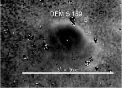
Figure 4.— DEM S159 shows blister-like features, exhibiting nebular traits for both high and low optical depth. As in Figure 3, the ratio of [S$\rm II$]/[O$\rm III$] reveals the presence of highly ionized gas (dark) in this region. This is confined to the northwest by a pronounced ionization transition zone, but not to the southeast.

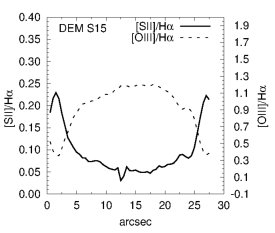
(a) DEM S15

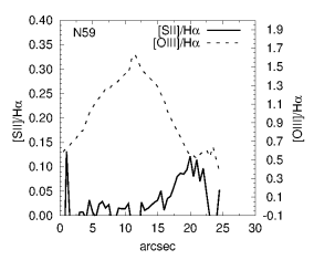
(b) N59

Figure 5.— The spatial profiles of [O$\rm III$]/H$\alpha$ and [S$\rm II$]/H$\alpha$ across the center of the optically thick object DEM S15 (top) and optically thin region N59 (bottom).

Finally, ionization-parameter mapping also constrains the optical depth in the line of sight, since the low-ionization, transition zone should also exist along these photon paths in an optically thick nebula. This was explored by Pellegrini et al. (2011) who found a lower limit of [S$\rm II$]/H$\alpha$ $\sim 0.05$ for LMC nebulae that are optically thick in the line of sight. Lower values of [S$\rm II$]/H$\alpha$ indicate that the low-ionization transition zone is missing or depleted, and therefore that the region is optically thin to the Lyman continuum. In Figure 5 we compare the line of sight emission line ratios of DEM S15 and N59, a pair of optically thick and optically thin Hii regions. DEM S15 is a classical Strömgren sphere, limb-brightened in the lower ionization species, and it shows a central line-of-sight [S$\rm II$]/H$\alpha$$=0.05$, consistent with an optically thick nebula of SMC metallicity. In contrast, in N59, the central [S$\rm II$]/H$\alpha$ ratio is essentially zero across much of the object, and thus no transition zone is seen in those sight lines, demonstrating that the object is optically thin.

2.2. Limitations for 2-ion mapping

Ionization-parameter mapping is tremendously powerful, and can even be done with only two radially varying ions. When using only two ions, we caution that the technique has three limitations. Ostensibly, the most important quantity to be derived with this technique is the escape fraction of LyC photons from an individual Hii region, $f_{\rm{esc}}$  defined as

$$\mbox{$f_{\rm{esc}}$}=e^{-\mbox{$\tau_{\rm LyC}$}}\quad.$$ (1)

Ionization-parameter mapping based on only two ions can provide only lower limits on $f_{\rm{esc}}$, because the observed morphology becomes degenerate at high $f_{\rm{esc}}$. This can be seen in the bottom row of Figure 2 for $\tau_{\rm LyC}\leq 1.0$, which corresponds to $\mbox{$f_{\rm{esc}}$}\geq 40\%$. In these cases, background emission masks the very faint, lower-ionization emission lines in fully ionized gas, and the ratio ceases to directly track changes in the Hii region ionization structure. This problem worsens as $T_{\rm eff}$ increases, and it becomes more difficult to identify the transition to neutral gas. However, only the hottest ionizing stars in the local universe will have $\mbox{$T_{\rm eff}$}\sim 44,500$ K, and when three ions are available, the degeneracies are resolved.

There is also a degeneracy between optically thin nebulae ionized by cool stars ($T_{\rm eff}\lesssim 34,000K$) and optically thick regions heated by hotter stars. The degeneracy exists where cool stars do not emit much radiation above 35 eV to generate O²⁺, and so these nebulae are entirely dominated by O⁺. Again, ionization parameter mapping based on three ions, adding S²⁺ for example, can resolve the degeneracy (Figure 1). However, we stress that this problem applies primarily to the lowest-luminosity objects, and as we show below, their aggregate luminosity is insignificant compared to the total amount of energy found to be escaping all Hii regions.

Finally, we again caution that for a population of randomly oriented blister Hii regions, it is likely that the orientation of some objects will cause a projected ionization-parameter gradient that appears optically thick on the limb, but is optically thin in the line of sight. The most extreme example is of a half-sphere, blister nebula viewed directly face-on: despite having $\mbox{$f_{\rm{esc}}$}=0.5$, the projected region is circular and will show an ionization transition zone associated with the optically thick half. However, as discussed in §2.1, the ionic ratios of [S$\rm II$], [O$\rm III$], and H$\alpha$ across the central region of these nebulae should show a deficit in lower-ionization species that is incompatible with optically thick models (Figure 5(b)). With further constraints on the ionizing SED and a quantitative evaluation of these ratios, we can still measure their optical depth. Thus, there may be instances where optically thin Hii regions are initially misidentified as optically thick, but these can be identified by quantitative examination of spatially resolved ionic ratios. If objects are misidentified, this again would favor underestimates of $\tau_{\rm LyC}$.

Table 1MCELS 1-$\sigma$ surface brightness detection limits

	${S(\rm H\alpha)}$	${\rm EM(H\alpha)}$	${S(\mbox{[O$\rm III$]})}$	${S\mbox{[S$\rm II$]})}$
Galaxy	${\rm\mbox{${\rm erg\ s^{-1}}$}\ cm^{-2}arcsec^{-2}}$	${\rm pc\ cm^{-6}}$	${\rm erg\ s^{-1}\ cm^{-2}\ arcsec^{-2}}$	${\rm erg\ s^{-1}\ cm^{-2}\ arcsec^{-2}}$
LMC	$7.0E-18$	3.5	$1.4E-17$	$5.2E-18$
SMC	$7.2E-18$	3.6	$5.4E-17$	$1.0E-17$

Note. — Values shown are the 1-$\sigma$ uncertainties in a single pixel for surface brightness and emission measure as shown. The LMC data are not continuum-subtracted and have a pixel scale of 3 arcsec, while the SMC data are continuum subtracted and have a pixel scale of 2 arcsec.

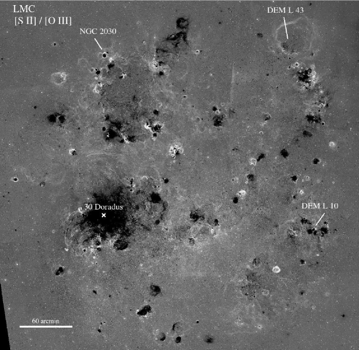
Figure 6.— The map of log [S II]/[O III] for the entire LMC galaxy created from the MCELS narrow-band imaging data. Black corresponds to low [S II]/[O III]; this ratio map is not based on continuum-subtracted data. North is up, east to the left in the center of the field.

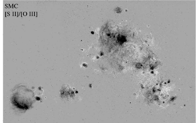
Figure 7.— Same as figure 6 for the SMC galaxy. This ratio map is based on continuum-subtracted data.

Hence, the caveats identified above can be resolved by ionization-parameter mapping in three ions and quantitative evaluation of the entire nebular projection. We note that these fairly manageable issues all work to underestimate the optical depth of Hii regions. Thus, ionization-parameter mapping shows great promise as a powerful tool in studies of the ISM. Emission-line ratio maps neutralize variations in surface brightness, clearly revealing changes in ionization structure for bright and faint regions alike. The power of the technique is that it allows us to identify optically thin Hii regions by the absence of the low-ionization envelope, which almost always indicates that the nebula is density-bounded.

3. Ionization-Parameter Mapping of the LMC and SMC

We now apply our technique of ionization-parameter mapping to the Large Magellanic Cloud (LMC) and Small Magellanic Cloud (SMC), which have been mapped with narrow-band emission-line imaging by the MCELS survey. This is a spatially complete, flux-limited survey carried out at the Cerro Tololo Inter-American Observatory (CTIO) with the University of Michigan’s Curtis 0.6/0.9m Schmidt telescope. Over the course of 5 years, the LMC and SMC were imaged in [S$\rm II$]$\lambda\lambda 6717,6731$, [O$\rm III$] $\lambda$5007, and H$\alpha$, with respective filter widths of 50, 40 and 30Å. The H$\alpha$ filter bandpass includes [N II]$\lambda\lambda$6548,6584 at a reduced throughput. The final product, mosaics in both low and high-ionization line emission, and in the H$\alpha$ recombination line, traces the ionized ISM at both large and small scales. The process of mosaicking the images resulted in a binned pixel scale of 3.0 and 2.0 arcsec pixel^-1 for the LMC and SMC, respectively. These correspond to a spatial scale of 0.7 pc and 0.6 pc for distances of 49 kpc  (Macri et al., 2006) and 61 kpc (Hilditch et al., 2005), respectively, with an effective resolution of $\sim 5$ arcsec. The 1-$\sigma$ surface-brightness limit of each band is listed in Table 2.2. These are the sensitivities per pixel, expressed as surface brightness in $\rm\mbox{${\rm erg\ s^{-1}}$}\ cm^{-2}~{}arcsec^{-2}$ and H$\alpha$ emission measure (EM) in $\rm pc\ cm^{-6}$. Such depth is important to form a complete understanding of the WIM ionization, and the dependence of $f_{\rm{esc}}$ on star-formation intensity and Hii region properties.

The MCELS survey includes continuum observations centered at 5130 Å and 6850 Å, with effective bandpasses of 155 Å and 95 Å , respectively. These were used to produce a continuum-subtracted mosaic of the SMC (Winkler et al., 2005). Based on spectrophotometric observations of the SMC region NGC 346 by Tsamis et al. (2003), we estimate that the flux calibration of the continuum-subtracted data has uncertainties on the order of 20%. At present, the LMC data are not yet continuum-subtracted. To flux-calibrate the LMC data, we used spectrophotometric observations by  Pellegrini et al. (2010), extracting MCELS line fluxes along the length of slit position 5 in that paper to determine the flux constants. We also compare against the flux-calibrated, narrow-band data obtained on the SOAR telescope in a 30 arcsec circular aperture at the position, $\alpha=$ 05:38:56.9, $\delta=$–69:05:21.8 (J2000) (Pellegrini et al., 2010). We find that the comparisons agree within approximately 20%, which then corresponds to the systematic uncertainty in our flux calibration.

We generated line-ratio maps of [S$\rm II$]/[O$\rm III$] for both the LMC and SMC using IRAF, with the LMC maps based on non-continuum-subtracted emission-line images, and the SMC maps based on continuum-subtracted images. These ratio maps, which probe the ionization parameter in the ionized gas, are shown in Figures  6 and  7, respectively.

3.1. Ionization-based HII region catalogs

Ionization-parameter mapping allows us to assign physically-motivated Hii region boundaries in complex, confused regions with multiple ionizing sources. In areas where Hii regions are overlapping, or are found in complex ionized backgrounds, the ionization stratification makes it possible to isolate individual photoionized regions, which is impossible with imaging in only H$\alpha$ or any single line. In particular, ionization-parameter mapping allows us to define nebular boundaries based on both ionization structure and H$\alpha$ surface brightness $S$(H$\alpha$) morphology. The examples in Figure 8 demonstrate how ionization-parameter mapping generates contrast between the DIG and low surface-brightness, extended Hii regions that are independently ionized entities. In the H$\alpha$ image (right panel of Figure 8), the objects DEM S10 and DEM S49 are amorphous regions that blend into the surrounding DIG with ambiguous boundaries. In contrast, the [S$\rm II$]/[O$\rm III$] ratio map clearly shows them as distinct regions. The boundaries of optically thick objects are usually unambiguous because these are characterized by a stratified ionization structure as described above, accompanied by a sharp decrease in surface brightness.

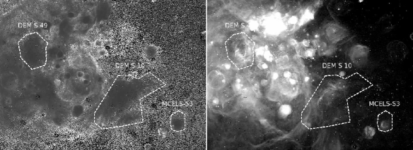
Figure 8.— [S$\rm II$]/[O$\rm III$] ratio map (left) and H$\alpha$ (right) for an SMC region, demonstrating the advantage of using [S$\rm II$]/[O$\rm III$] in combination with H$\alpha$ to define the boundaries of extended Hii regions coincident with complex background structures (e.g., DEM S49), and those with extended, faint emission (e.g., DEM S10, MCELS-S3). We indicate Hii region boundaries for DEM S10, DEM S49 and MCELS-S3 with dashed lines in both images.

Since previous nebular catalogs for the Magellanic Clouds are based only on H$\alpha$ morphology (e.g., Henize 1956; Davies et al. 1976), we use these more sophisticated criteria based on ionization-parameter mapping to compile a more physically-based catalog of Hii regions in these galaxies. In the case of extended, optically thin objects that show only gradual changes in [S$\rm II$]/H$\alpha$ or [S$\rm II$]/[O$\rm III$], we define the Hii region boundary to be the point at which either the $S{\rm(H\alpha)}$ or the ionic ratio become indistinguishable from the DIG, whichever is larger in size. We defined photometric apertures with polygons in SAOImage DS9, for both target objects and local background regions; we used the FUNCNTS routine from FUNTOOLS to measure the fluxes.

The photometry of faint objects, especially seen in [S$\rm II$] and [O$\rm III$] filters, are at risk of being contaminated by stellar continuum in the LMC, where our data are not continuum subtracted. We minimize this contamination by avoiding foreground Galactic stars and also sampling the local density of field stars with our background apertures. Despite the careful creation of apertures, the difference between stellar populations inside and outside the HII regions may still introduce significant errors, since the most massive, brightest stars often reside within HII regions. Thus, errors in the background subtraction dominate the flux uncertainties for both galaxies, and they are largest for low surface-brightness objects. We therefore find that the median local background surface brightness for nebulae in the LMC is larger than for the SMC: $7.0\times 10^{-16}$ and $1.3\times 10^{-16}\ \rm erg\ s^{-1}cm^{-2}arcsec^{-2}$, respectively, in H$\alpha$. However, we stress that high surface-brightness emission dominates most objects, yielding median background uncertainties of 6% and 8% in the LMC and SMC, respectively. For the LMC, the discrete stellar contributions can increase this uncertainty to about 18%. This is consistent with a comparison of our background-subtracted fluxes of bright, isolated LMC and SMC Hii regions to their fluxes reported by Kennicutt et al. (1989). We find that the independent measurements agree within 20%, which now also includes systematic uncertainties.

We further explored the limiting case of applying a constant background to all objects. For the LMC, we calculated this background from the mean of three locations, two in the north and one in the south to estimate the contamination from sources producing a constant background such as the sky, large scale diffuse emission, etc. We find the mean, constant background $S{(\mbox{H$\alpha$})}=5.2\times 10^{-16}\ \rm erg\ s^{-1}cm^{-2}arcsec^{-2}$. For the SMC, we determined the background of the continuum-subtracted H$\alpha$ image to be consistent with zero ($7\times 10^{-18}\pm 7\ \rm erg\ s^{-1}cm^{-2}arcsec^{-2}$; cf. Table 2.2). For both galaxies, subtracting the median backgrounds affects the resulting $L$ by no more than 0.2 dex, and does not substantively change our results.

Our Hii region catalogs for the LMC and SMC defined with these ionization-based criteria are presented in Appendix B, Tables LABEL:tab:LMCObjs and LABEL:tab:SMCObjs, which give luminosities and associated Hi column densities for 401 objects in the LMC, and 214 in the SMC.

3.2. The HII region Luminosity Function

We find that our Hii region boundaries and H$\alpha$ luminosities generally agree with those determined in previous, H$\alpha$-only studies by, e.g., Kennicutt et al. (1989), including the substructure in most of the DEM (Davies et al., 1976) and Henize (1956) surveys. This is especially true for simple objects with a low local background. Figures 9(a) and 9(b) show the differential Hii region luminosity functions (Hii LF) for our new LMC and SMC catalogs, respectively (squares), together with those generated by Kennicutt et al. (1989) (crosses), fitted above $\log\mbox{$L$}=37.0$ (where not explicitly stated, the units of $L$ are ${\rm erg\ s^{-1}}$). The power-law slope of the LMC Hii LF reported by Kennicutt et al. is $B=1.75\pm 0.15$, where

$$dN(\mbox{$L$})\ \propto\mbox{$L$}^{-B}d(\mbox{$L$})\quad.$$ (2)

This is statistically consistent with the fitted Hii LF slope for our data, $B=1.79\pm 0.08$. An identical analysis for the SMC, as shown in Figure 9(b), yields an Hii LF slope of $B=1.88\pm 0.09$, for our new catalog, compared to a reported slope of 1.9 from Kennicutt et al. (1989). Thus, although previous measurements of the Hii LF do not use our ionization-based criteria, they result in essentially identical LF slopes.

Both Magellanic Cloud Hii LF slopes flatten around $\log~{}\mbox{$L$}=37.0$, which is equivalent to $Q{\rm(H^{0})}=48.9~{}\rm s^{-1}$. This flattening is observed in other galaxies whose Hii LFs probe $\log~{}\mbox{$L$}<36.0$, including the Milky Way (Paladini et al., 2009), M51 (Lee et al., 2011) and M31 (Azimlu et al., 2011). The observed flattening of the Hii LF in this regime was predicted in Monte Carlo simulations by Oey & Clarke (1998) and Thilker et al. (2002), and it is caused by stochastic ionizing populations at these low luminosities. For comparison, $\log~{}\mbox{$L$}=37.0$ is the luminosity of the Orion Nebula, whose parent ionizing cluster has a mass of 4500 ${\cal M}_{\odot}$(Hillenbrand & Hartmann, 1998), dominated by a single O6.5 V star.

A final caveat: at the lowest luminosities, there is a decrease in the Hii LFs. This is clearly established for $\log~{}\mbox{$L$}<36.5$ in both galaxies. The drop in source counts could be an indication that below this $L$ we are not complete. Alternatively, since the stellar ionizing fluxes plummet strongly for stars later than early B spectral types, this turnover in the Hii LF signals an intrinsically different class of ionizing sources and nebular objects. These must include individual Hii regions of later B-type stars, and perhaps some faint, optically thin nebulae that are intrinsically weak in recombination lines due to their low optical depth. There also may be some shock-heated filaments, although we tried to avoid most of these. Planetary nebulae should not be important above $\mbox{$L$}\sim\rm 5e35~{}\mbox{${\rm erg\ s^{-1}}$}$ (Azimlu et al., 2011).

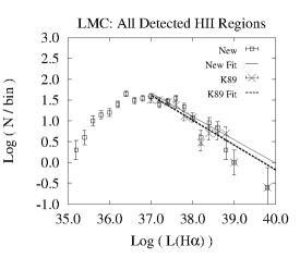
(a) LMC

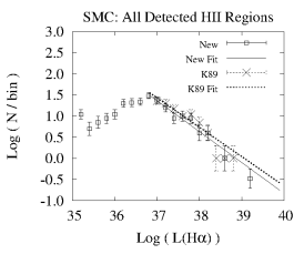
(b) SMC

Figure 9.— The LMC (panel $a$) and SMC (panel $b$) Hii LFs for our catalogs of photoionized Hii regions (squares), and from Kennicutt et al. (1989)(crosses). Power law fits to the data, weighted by inverse error, are shown with the solid and dotted lines, respectively, for our data and those of Kennicutt et al. The error bars show the root-$N$ uncertainties.

3.3. An enigmatic, highly ionized region

The technique of ionization-parameter mapping is effective at highlighting large, extremely faint structures. The [S$\rm II$]/[O$\rm III$] ratio map of an LMC object at $\alpha=$ 04:55:50 $\delta=$ 67:30:50 (J2000) is shown in the left panel of Figure 10, with an inner ellipse to mark the extent of highly ionized and filamentary gas. The middle panel shows a larger contour that highlights an HI cavity seen in the Hi data of Kim et al. (2003) with a major axis of 550 pc and Hi column density $N{\rm(HI)}$ $=0.6\times 10^{21}~{}{\rm cm^{-2}}$. Both ellipses have the same orientation suggesting they are related. The right panel of Figure 10 shows faint H$\alpha$ emission is co-spatial with the [O$\rm III$], while no [S$\rm II$] was detected. This indicates that the optically emitting gas is fully ionized. This structure is intriguing because the [S$\rm II$]/[O$\rm III$] morphology is similar to optically thin nebulae ionized by OB stars, yet no ionization sources are known in the region, nor is there evidence of a prior supernova or shocked gas. The size and faintness of this highly excited region, together with the lack of an ionization source, make this object unique. Further observations to identify its nature and origin are required.

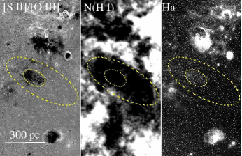
Figure 10.— A large, highly ionized bubble with no known ionization source. Left: [S$\rm II$]/[O$\rm III$] ratio map; Center: Hi column density map of the region, with white showing Hi emission; Right: The region in H$\alpha$. All panels are shown with the same scale, where north is up and east left. The central contour marks the boundary where the object is indistinguishable from the background, while the larger contour marks the rim of the bubble seen in $N{\rm(HI)}$.

4. Optical Depth of the H II Regions

From the diagnostics based on ionization structure as described in §2, we classify the optical depth of our individual, catalogued Hii regions into the following categories: (0) indeterminate, (1) optically thick, (2) blister, (3) optically thin, and (4) shocked nebulae. These are given in Column 4 of Tables LABEL:tab:LMCObjs and LABEL:tab:SMCObjs. Class 0 objects, with indeterminate optical depth, fall into two categories: those which lack [O$\rm III$] emission, causing a high [S$\rm II$]/[O$\rm III$] ratio, with little ionization structure; and large scale, diffuse structures. This latter category is difficult to define morphologically, but since many objects in the DEM LMC catalog include these features, we have attempted to catalog them as well.

We define optically thick objects (class 1) to be those showing classic, low-ionization envelopes enclosing at least 2/3 of the central, high-ionization regions in projection, as described in §2. Blister nebulae (class 2) are defined by a low-ionization envelope that surrounds between 1/3 and 2/3 of the observed object; additionally, objects having complex internal ionization fronts with extended [O III] emission are treated as blisters. Optically thin (class 3) objects show low [S$\rm II$]/[O$\rm III$] throughout, with low-ionization envelopes covering $<$ 1/3 of the highly ionized gas (see Figures 3 and 4). Shocked objects (class 4) are characterized by an ionization structure which is inverted relative to photoionization, i.e. these objects are have enhanced [O$\rm III$] emission surrounding strong [S$\rm II$]. Our survey is not intended to be complete with respect to shocked objects, and we typically avoided cataloguing them. Since these are not photoionized, they are excluded from further consideration. Additional general classification criteria include gradients in ionization parameter, the detection of ionization fronts distinct from the background, and the ionized extent of the object. Radial projections of the [S$\rm II$]/[O$\rm III$] ratio, were made to assess the significance of specific individual features that were identified. Three of the authors (EWP, JZ, and AEJ) used these criteria to carry out independent classifications of all the objects. To arrive at a final catalog, we resolved the differences by discussing specific key features and quantitatively measuring the optically thin covering fraction.

We roughly estimate the LyC escape fraction $f_{\rm{esc}}$ for each object in classes (1) – (3) as follows: optically thick objects are assigned $\mbox{$f_{\rm{esc}}$}=0$; optically thin objects are assigned $\mbox{$\tau_{\rm LyC}$}=0.5$, which corresponds to $\mbox{$f_{\rm{esc}}$}=0.6$; and blister objects are assigned a value of $f_{\rm{esc}}$ that is half that for the optically thin objects, namely, $\mbox{$f_{\rm{esc}}$}=0.3$. Since we have observations in only two diagnostic ions, some of the class 3 objects in reality may be quite optically thin (§2.2), and so we compare these estimates to direct measurements of optical depths using data from Voges et al. (2008), who compared the observed $L$ to predicted values based on the spectral types of individual ionizing stars for a sample of LMC Hii regions. Although, as mentioned earlier, there is considerable uncertainty in optical depth estimates based on this method, it remains the most direct, quantitative way to check our results based on ionization-parameter mapping.

Voges et al. (2008) adopted ionizing fluxes from the WM-basic models of Smith et al. (2002). These SEDs are intermediate in hardness among the different available, modern codes, and they best fit the observed nebular emission-line spectra (Zastrow et al., 2011a). Due to the large uncertainty in determining spectral types of O stars from photometry alone, we restrict our comparison with the Voges et al. (2008) sample (their Tables 1 and 3) to objects having stellar spectral types determined at least in part by spectroscopic classifications, with a further requirement that at least half of the derived ionizing luminosity is attributed to stars with spectroscopic spectral types. These include a reanalysis of Hii regions from Oey & Kennicutt (1997), which is based entirely on spectroscopic classifications with individually measured reddenings, listed in Table 1 of Voges et al. We exclude DEM L 7, L 9 and L 55 because they are class 0 objects, and DEM L 229, which displays evidence of shock excitation.

Using the predicted H$\alpha$ luminosities from Voges et al. (2008), and our new observed H$\alpha$ luminosities, we calculate individual $f_{\rm{esc}}$ values for each nebula according to

$$f_{\rm esc}=1-L_{\rm obs}/L_{\rm predicted}\quad.$$ (3)

The predicted luminosity is derived from the expected rate of ionizing photons $Q{\rm(H^{0})}$ assuming each absorbed LyC photon will result in 2.2 H$\alpha$ photons. In Table 2, we present the $f_{\rm{esc}}$ values for the 13 Hii regions, comparing the rough estimates obtained from ionization-parameter mapping as described above with measurements based on the data of Voges et al. (2008). Column 1 gives the DEM identifier for each object, and column 2 gives our crude $f_{\rm{esc}}$ estimated from ionization-parameter mapping, as described above. Column 3 gives $f_{\rm{esc}}$ estimates based on data from Voges et al. (2008) with values derived from known stellar spectral types.

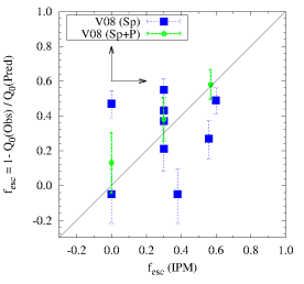
Figure 11.— Our $f_{\rm{esc}}$ values estimated from ionization-parameter mapping plotted against $f_{\rm{esc}}$ calculated from observed and predicted ionization rates from Voges et al. (2008). The values of $f_{\rm{esc}}$ derived from both methods are lower limits, illustrated by the orthogonal set of arrows.

Figure 11 plots the comparison between $f_{\rm{esc}}$ estimated from our classification of optical depth based on ionization-parameter mapping and the measured values based on the data of Voges et al. (2008). There is a general agreement between our crude estimates for $f_{\rm{esc}}$ based on ionization-parameter mapping and the measured values based on the observed ionizing stars, for all but 1 object; the standard deviation from the identity relation is $\sigma=0.23$, excluding DEM L 293 (see below). Although, as discussed in §2.2, our values for $f_{\rm{esc}}$ are all lower limits, especially for objects categorized as optically thick, and the $f_{\rm{esc}}$ values derived using Voges et al. (2008) are also lower limits, the surprisingly good correspondence suggests that both methods actually yield reasonable estimates of the optical depth.

The Voges et al. escape fraction of DEM L 293 is –1.52, which is an unphysical value, placing it far beyond the bounds of the plot in Figure 11. The predicted ionizing luminosity in DEM L 293 is observationally attributed to only a single O3 III star. However, given the typical cluster mass in which O3 III stars form, additional, obscured or overlooked ionization sources in this cluster are likely to be present. In particular, Walborn et al. (2002) identified an odd semi-stellar source within DEM L 293 which is brighter than the single O3 III star. If the ionizing luminosity of this source is equal to an O3 III star then the V08 $f_{\rm{esc}}$ would then be -0.52, much closer to the $f_{\rm{esc}}$ value derived from ionization-parameter mapping.

Overall, however, our extremely crude estimates of $f_{\rm{esc}}$ based on ionization-parameter mapping show surprisingly good agreement with the empirically measured $f_{\rm{esc}}$. In spite of the fact that our estimates tend to yield lower limits, the general agreement confirms that objects appearing to be optically thick indeed tend to be radiation-bounded. As mentioned in §2.1, this is also supported by their morphologies, which generally resemble smooth, Strömgren spheres. Furthermore, the occurrence of optically thick objects that appear to be density-bounded is extremely rare, since this only happens occasionally for the very hottest spectral types (e.g., Figure 2). Figure 11 thus demonstrates the general viability of ionization-parameter mapping as a diagnostic of nebular optical depth.

Table 2Comparison of $f_{\rm{esc}}$ estimates

Object	$f_{\rm{esc}}$(IPM)a	$f_{\rm{esc}}$(V08)b
DEM L 10Bc	0.38	-0.05
DEM L 13	0.30	0.38
DEM L 31	0.60	0.49
DEM L 34	0.30	0.55
DEM L 68c	0.59	0.58
DEM L 106	0.30	0.37
DEM L 152+156	0.56	0.27
DEM L 196c	0.03	0.13
DEM L 226	0.00	-0.05
DEM L 243	0.00	0.47
DEM L 293	0.30	-1.52
DEM L 301	0.30	0.21
DEM L 323+326	0.30	0.43

Note. —

^a $f_{\rm{esc}}$ derived via ionization-parameter mapping.

^b $f_{\rm{esc}}$ derived from predicted H$\alpha$ fluxes from Voges et al. (2008) and equation 3.

^c Composite objects whose $f_{\rm{esc}}$ values reflect the luminosity-weighted contributions of individual optically thin and thick subregions.

4.1. Optical depth and H$\alpha$ luminosity

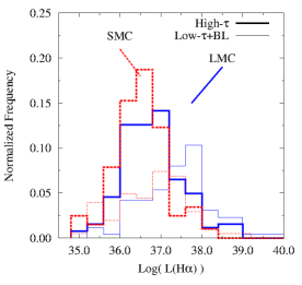
Figure 12.— The LFs for optically thin nebulae, including blister objects; and optically thick nebulae, shown with thin and thick lines, respectively. The LMC distributions are shown with solid lines (blue) and the SMC are shown with dashed lines (red).

Table 3Median H II Region Properties

	LMC				SMC
Class	No.	%a	$L$	$N{\rm(HI)}$	No.	%a	$L$	$N{\rm(HI)}$
			$10^{36}\ \rm erg\ s^{-1}$	$10^{21}\ \rm cm^{-2}$			$10^{36}\ \rm erg\ s^{-1}$	$10^{21}\ \rm cm^{-2}$
(0) Indeterminate	130	$\cdots$	3.7	1.8	7	$\cdots$	0.05	6.5
(1) Opt Thick	158	60	3.6	2.8	132	62	2.1	6.4
(2) Blister	58	18	18.8	1.9	41	19	4.7	5.1
(3) Opt Thin	46	22	19.7	2.0	30	14	4.0	6.2
(4) Shocked	9	$\cdots$	15.6	1.8	4	2	1.5	5.7
(2) $+$ (3)	104	40	19.2	1.9	71	33	4.5	5.3
(1)$+$(2)$+$(3)	262	100	5.5	2.5	203	100	2.6	5.9

Note. — ^aPercentages are calculated for photoionized objects, based on total values in the bottom row.

Table 3 summarizes the median nebular properties for each optical depth class as catalogued in Tables LABEL:tab:LMCObjs and LABEL:tab:SMCObjs. Column 2 gives the number of objects in each class in the LMC. Column 3 gives the corresponding percentage of the total number of objects that are clearly photoionized, thus excluding class 0 and class 4 objects from the total numbers of photoionized nebulae. Columns 4 and 5 give the median $L$ and median $N{\rm(HI)}$ (see §4.2 below) associated with the objects, respectively. Columns 6 – 9 list the same quantities for the SMC.

Figure 12 shows the $L$ distributions for the LMC (solid, blue line) and SMC (dotted, red line), of optically thin nebulae (thin lines) and optically thick nebulae (thick lines). The optically thin data include blister Hii regions as defined above. The distributions are normalized by the number of Hii regions in the last row of Table 3. Figure 12 and Table 3 show that for both galaxies, the $L$ distributions for optically thick objects peak at lower luminosities than those for the optically thin ones. This difference is larger in the LMC, producing a bimodal distribution, with the median $L$ for optically thin nebulae 5 times brighter than for the optically thick ones (Table 3). The median $L$ of optically thin SMC nebulae is only twice that of optically thick ones, as expected given the lower star-formation rate in that galaxy, and fewer luminous Hii regions. However, the $L$ distributions for the different classes are similar between the two galaxies, showing peaks near similar values and similar ranges in luminosity. The role of dust in these trends is unclear. It is possible that two Hii regions with similar ionizing luminosities will have different $f_{\rm{esc}}$ if one has more dust than the other. This could explain the coexistence of optically thin and thick regions in the same luminosity bin.

In Figure 13, we plot the frequencies of optically thin nebulae as a function of $L$. Both galaxies exhibit a clear increase in the frequency of optically thin nebulae with increasing H$\alpha$ luminosity. However, we stress that both optically thick and thin objects are found at almost all luminosities having $\log~{}\mbox{$L$}<39.0$. Table 3 also shows that the frequencies of optically thin objects, including blisters, are similar between the two galaxies, 40% and 33% in the LMC and SMC, respectively. Furthermore, there is a transition luminosity above which optically-thin nebulae dominate, $\log~{}\mbox{$L$}=37.0$, occurring at the same luminosity in both galaxies. Beckman et al. (2000) speculated that such a transition is responsible for possible discontinuities observed near $\log~{}\mbox{$L$}=38.6$ in extragalactic Hii LFs, but our data clearly show that optically thin objects dominate at luminosities a full 1.6 dex lower in $L$.

It will be interesting to see how strongly our transition value of $\log~{}\mbox{$L$}=37.0$ depends on galaxy properties. This relatively low luminosity corresponds to nebulae ionized stochastically by single O stars or substantially evolved associations and clusters (Oey & Clarke, 1998). Thus, most of the objects typically apparent in Figures 6 and 7, as well as those typically detected in local surveys (e.g. Thilker et al. 2002) are the more luminous Hii regions, which are mostly, but not all, optically thin. The most luminous objects have the highest likelihood of being optically thin, including 30 Doradus in the LMC, and the N66 in the SMC. These are indeed found to be optically thin in our study, a result consistent with the findings of Pellegrini et al. (2011) in 30 Dor, and the low optical depths found for other giant extragalactic Hii regions (e.g., Castellanos et al., 2002).

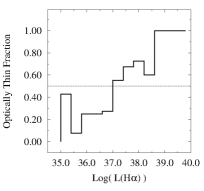
(a) LMC

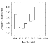
(b) SMC

Figure 13.— The fraction of optically thin Hii regions as a function of $L$ is shown for the LMC and SMC in panels 13(a) and 13(b), respectively. Optically thin objects dominate above a fraction of 0.5, indicated by the horizontal dotted line. The lowest-$L$ bins likely include contamination by planetary nebulae.

4.2. Relation with the Neutral ISM

The neutral ISM represents the default environment into which ionizing photons from optically thin regions are deposited, and its properties are fundamental to the radiative transfer of the Lyman continuum. The Magellanic Clouds were mapped in Hi with the Australia Telescope Compact Array by Kim et al. (2003) (LMC) and Stanimirović et al. (1999) (SMC). The LMC Hi data have 60 arcsec resolution over the ${\rm 11.1^{\circ}\times 12.4^{\circ}}$ survey area; the SMC Hi data have a resolution of 98 arcsec over the ${\rm 5^{\circ}\times 5^{\circ}}$ field. The LMC is a face-on disk galaxy, while the SMC has a more amorphous, three-dimensional irregular morphology. We now explore the relationship between nebular optical depth and the neutral ISM.

Figure 14 traces the propagation of radiation in the LMC (top) and SMC (bottom) using [S$\rm II$]/[O$\rm III$] (red), [O$\rm III$]/H$\alpha$ (blue) and $N{\rm(HI)}$ (green). The contrast in ionization morphology between the two galaxies is striking. As ionizing radiation enters the diffuse ISM, it encounters a combination of ionized and neutral gas. The LMC neutral disk has been disrupted, forming shells and filaments surrounding the ionized gas (Kim et al., 1998). These structures are believed to be the result of stellar feedback acting on the ISM (e.g. Oey & Clarke 1997). Often, optically thin Hii regions line the edges of large Hi shells, radiating LyC photons into their interiors. A few examples are highlighted with arrows in the LMC (Figure 14). These large-scale Hi structures appear to allow ionizing radiation to travel hundreds of pc without being absorbed.

The SMC, on the other hand, has a less fragmented Hi structure (Stanimirović et al., 1999). The neutral ISM in this galaxy is much more diffuse and less filamentary than that in the LMC (Oey, 2007). Intense and vigorous star formation is at the center of the two most prominent Hi masses. The first is coincident with N66 near the northern boundary of the galaxy. Lines of sight toward this optically thin region show that $N{\rm(HI)}$ anti-correlates with highly ionized gas (Figure 14). Thus, in this region, Hi is being disrupted by the ionizing radiation entering the diffuse ISM. The second region is located in the SW portion of the galaxy. Despite a high $N{\rm(HI)}$, this region contains many optically thin nebulae, which form a large complex filled with a highly ionized DIG. To improve our sensitivity to ionization transitions in the DIG, we applied an $11\times 11~{}\rm arcsec^{2}$ median filter to the [S$\rm II$] and [O$\rm III$] data, creating a smoothed [S$\rm II$]/[O$\rm III$] map. The region is seen in Figure 15 in the inverted map (left) and $N{\rm(HI)}$ (right). The enhanced sensitivity reveals an ionization transition zone coincident with the edge of the Hi distribution. Thus, the Hi gas appears to be trapping the ionizing radiation, while individual nebular $f_{\rm{esc}}$ depends on the detailed morphology.

Given the strong morphological contrast between the two galaxies, in the Hi properties and star-formation intensity, the quantitative similarities in the nebular optical depths found above in §4 are surprising. In particular, despite expectations that the reduced $N{\rm(HI)}$ and higher star-formation intensity of the LMC would lead to more optically thin nebulae, we saw above that the relative frequency of optically thin and thick objects are similar between the two galaxies (Table 3). It will be important to see whether other galaxies also yield similar relative frequencies.

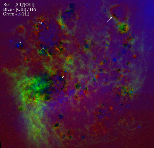
(a) LMC

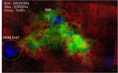
(b) SMC

Figure 14.— Composite images of the LMC (top) and SMC (bottom), which contrast the different ISM structure seen in the two galaxies. [O$\rm III$]/H$\alpha$ (blue), [S$\rm II$]/[O$\rm III$] (red), and $N{\rm(HI)}$ (green) respectively trace high-excitation nebulae, low-excitation gas, and neutral gas along the line of sight.

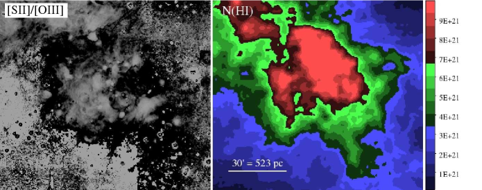
Figure 15.— The southwest region of the SMC in [S$\rm II$]/[O$\rm III$] (left), smoothed with an $11\times 11\ \rm arcsec^{2}$ median filter. We have inverted the gray scale to better highlight low-ionization regions, thus black corresponds to areas of low ionization. Surrounding the entire complex is an ionization transition zone (black). This transition zone is coincident with the boundaries of a massive Hi cloud seen in the $N{\rm(HI)}$ map of Stanimirović et al. (1999) (right).

4.3. Optical Depth and $N{\rm(HI)}$

Figure 16 shows the $N{\rm(HI)}$ distribution for optically thin (thin lines) and thick nebulae (thick lines) for the LMC (solid blue lines) and SMC (dotted red lines). We used the $N{\rm(HI)}$ maps of Kim et al. (2003) for the LMC and Stanimirović et al. (1999) for the SMC, to average the $N{\rm(HI)}$ within the individual Hii region apertures for each object, as defined in §3.1. We caution that these measurements correspond to the $N{\rm(HI)}$ along the line of sight toward the objects. Because the SMC has a more three-dimensional geometry than the LMC, which is an almost face-on disk, the $N{\rm(HI)}$ measurements for the SMC include a larger contribution from foreground and background ISM than in the LMC. However, we note that the SMC metallicity and dust content are only one-fifth that of the LMC; thus, for the same $N{\rm(HI)}$, $\tau_{\rm LyC}$ will be lower in the SMC. Hence the less abundant dust may somewhat offset the effect of increased $N{\rm(HI)}$ in this galaxy. Still, because of the contrasting galaxy morphologies, the difference in median $N{\rm(HI)}$ between optically thin and thick populations within each galaxy is smaller than the difference in global median $N{\rm(HI)}$ between the two galaxies. Specifically, the median value of all LMC Hii regions is 2.4 times lower than in the SMC (Table 3), while the ratio of the median $N{\rm(HI)}$ for optically thick (class 1) to thin (class 2 $+$ 3) objects is 1.5 and 1.2 in the LMC and SMC, respectively. Figure 16 shows that, for both galaxies, the $N{\rm(HI)}$ distributions for optically thin and thick nebulae are similar to each other, but that the former are weighted more toward lower columns, as expected. However, we note that even in the LMC, which has minimal line-of-sight projection effects, the $N{\rm(HI)}$ distribution for optically thin objects extends up to $N{\rm(HI)}$ $=8\times 10^{21}{\rm cm^{-2}}$, a value as high as that for the optically thick ones.

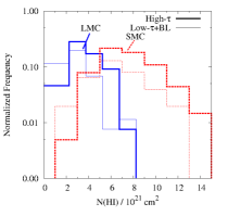
Figure 16.— The normalized $N{\rm(HI)}$ distributions for optically thin and optically thick nebulae, shown with thin and thick lines, respectively. The LMC and SMC distributions are shown with solid lines (blue) and dashed lines (red), respectively. These have been scaled by the total number of objects in each group.

In Figure 17 we show the relative frequency of optically thin nebulae as a function of $N{\rm(HI)}$ in the LMC and SMC. As expected, we see a strong decrease in the frequency of optically thin objects with increasing Hi column, although as emphasized above, there are still optically thin objects found near the highest $N{\rm(HI)}$. In both galaxies, there is a transition $N{\rm(HI)}$ below which optically-thin nebulae constitute the majority, at $3\times 10^{21}~{}{\rm cm^{-2}}$ in the LMC, and $6\times 10^{21}~{}{\rm cm^{-2}}$ in the SMC. The SMC transition $N{\rm(HI)}$ is two times higher than in LMC, which is consistent with the 2.4 times higher median $N{\rm(HI)}$ value for all Hii regions in the LMC relative to the SMC, due to line-of-sight ISM projection. Thus, in spite of the very different Hi morphology between the two galaxies, the quantitative relationship between nebular optical depth and Hi column is remarkably similar.

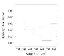
(a) LMC

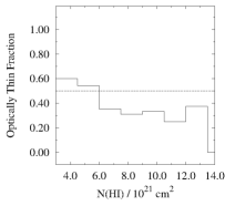
(b) SMC

Figure 17.— The frequency of optically thin Hii regions vs line-of-sight $N{\rm(HI)}$ within the object apertures, for the LMC and SMC in panels 17(a) and 17(b), respectively. Optically thin objects dominate above a fraction of 0.5, indicated by the horizontal dotted line.

5. Global Escape Fractions

While the frequency of optically thin vs thick Hii regions is similar in both galaxies, it is the structure of the diffuse ISM that ultimately determines how many ionizing photons heat the galaxy, and how many escape into the IGM, a quantity crucial to our understanding of cosmic evolution. Figure 14 highlights how, in comparison to the SMC, the evacuated ISM of the LMC allows the radiation produced in these regions to travel farther, and perhaps leave the galaxy. In the SMC much of the ionizing radiation escaping Hii regions is unable to penetrate the higher apparent Hi column. We now explore the global escape fractions for the Magellanic Clouds.

5.1. HII Region Location

Gnedin et al. (2008) highlighted the importance of Hii region location on the escape of ionizing radiation from galaxies. In the LMC and SMC, the largest and most luminous Hii regions are found toward the galaxy edges, and these objects are apparently optically thin. Take for example DEM S167, seen in the southeast extreme of the SMC (Figures 7 and 14(b)). In Figure 18 the transition in ionization is shown in [S$\rm II$]/[O$\rm III$] (left) coincident with the Hi shell SSH97 499 (Stanimirović et al., 1999) (right). These diagnostics indicate that part of the region is optically thick. However, there is [O$\rm III$] emission extending to the south, well beyond the ionization transition zone. The existence of extended [O$\rm III$] implies a large nebular escape fraction. The significance of escaping radiation from DEM S167 is amplified by its location near the edge of the SMC (Figure 14(b)).

Following Voges et al. (2008), we compare the expected H$\alpha$ luminosity from the stellar population to the observed value. The predicted H$\alpha$ luminosity from 7 known O stars, ranging from O4V to O9.5V, was derived using the observed relation between spectral type and $Q{\rm(H^{0})}$ from Martins et al. (2005). This includes a rare, well-studied WO4+O4 binary, for which we adopt the luminosities reported by St-Louis et al. (2005) equal to 75% of the total ionizing budget. The predicted H$\alpha$ luminosity is $\log L=38.137$, implying $f_{\rm{esc}}$$=27$%, consistent with our estimate of 30% from ionization-parameter mapping. As the eastern-most known SMC Hii region, its blister opens away from the galaxy, making it a prime candidate to contribute to the galactic escape fraction. The escaping UV radiation would be detectable only from certain directions as predicted by Gnedin et al. (2008).

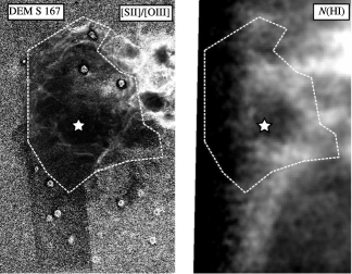
Figure 18.— The optically thin Hii region DEM S 167 located at the southeast boundary of the SMC. The left panel, showing [S$\rm II$]/[O$\rm III$], shows a strip running N-S with spuriously enhanced levels of [O$\rm III$]. However, extended [O$\rm III$] emission (black) is clearly detected beyond the southern nebular boundary, in excess of the artifact’s signal. The right panel shows the Hi column density map from (Stanimirović et al., 1999), demonstrating that the [O$\rm III$] emission extends beyond the Hi shell. The star indicates the location of the WO4+O4 binary, and the ionization-based boundary of the nebula is shown as a dashed line.

5.2. Hii region luminosity

The most luminous Hii  region in the LMC is 30 Doradus, ionized by the cluster R136a. It has a reddened luminosity of $\log~{}\mbox{$L$}={39.66}$, and it is ionized by hundreds of O stars. Similarly, at $\log~{}\mbox{$L$}=38.82$, the brightest nebula in the SMC is N66, ionized by at least 30 O stars in the cluster NGC 346. We can see in Figures 6 and 7 that these luminous objects are strongly optically thin, based on their very extended [O$\rm III$] emission. Furthermore, they are not deeply embedded in their respective galaxies, implying that these massive regions produce ionizing radiation that may escape into the IGM.

To examine the LyC photon path lengths from these two, luminous objects, we show the azimuthally averaged [S$\rm II$]/[O$\rm III$] ratio for these regions in Figure 19, centered on the main ionizing clusters R136a (top), and NGC 346 (bottom). Small, discrete Hii regions that are projected in the line of sight within these regions are excluded from the azimuthal averages in Figure 19. Figure 19 also shows the average radial $N{\rm(HI)}$. The profile of 30 Doradus is plotted to maximum radii where the gradient of both quantities is equal to zero, and marks the distance at which the ionizing radiation from these sources is no longer dominant. N66 is fainter, so it is less clear exactly where the influence of its ionizing source ends. Clearly, the extended [O$\rm III$] emission from the gas surrounding both objects requires a photoionizing source of high-energy photons from R136a and NGC 346, which dominate the ionization of the DIG out to at least 600 pc, whether or not this gas was ever associated with the Hii region, or is just part of the DIG. This is in agreement with the enhanced H$\alpha$ surface brightness of 30 Dor out to 850 pc noted by Kennicutt et al. (1995).

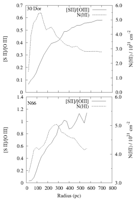
Figure 19.— The large-scale radial profiles of [S II]/[O III] and $N{\rm(HI)}$, averaged in annuli centered on R136a in 30 Dor (top) and NGC 346 in N66 (bottom). Nearby H II regions falling within the annuli were masked.

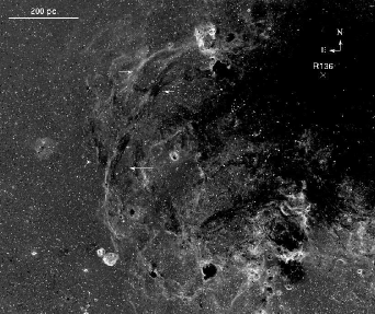
Figure 20.— The complex region east of R136a seen in [S$\rm II$]/[O$\rm III$]. R136a is marked in the upper right corner of the image. Marked by arrows are ionized filaments which exhibit ionization stratification over nearly 500 pc in length. The orientation of the stratification is evidence of a centrally located illuminating source at a location consistent with 30 Doradus.

Figure 19 shows that the peak $N{\rm(HI)}$ associated with optically thin objects can occur at radial distances that are well within the radial limits of the photoionized region. This suggests that the neutral and molecular ISM is highly inhomogeneous and clumpy, with large holes or clear areas that allow the escape of ionizing radiation. This situation is similar to the ionization cone detected in NGC 5253 (Zastrow et al., 2011b). In particular, the radial bins used to produce Figure 19 mask important features in the [S$\rm II$]/[O$\rm III$] and $N{\rm(HI)}$ distributions around 30 Doradus. These include narrow, radial projections containing continuous regions of highly ionized gas extending 1 kpc in various directions from 30 Doradus. There is no evidence for additional ionizing sources that can explain the extended ionization, so we argue that the variation in path length is due to variations in ISM density. East of the ionizing source, R136a, we see a complex of edge-on filaments (Figure 20), associated with the giant Hi shell LMC 2 (Meaburn, 1980). These filaments form a continuous arc over 500 pc in length, at a distance ranging from 0.6 and 0.8 kpc from R136a, with strong [O$\rm III$] facing the ionizing cluster, and strong [S$\rm II$] facing away from it, as shown by the arrows in the Figure. This ionic stratification confirms that the ionizing photons striking these filaments or sheets originate from R136a. Similar filaments are detected west of N66 (Figure 14(b)), opposite the bulk of the SMC. Unfortunately, our data do not extend far enough to look for filaments beyond DEM S167 in the direction away from the SMC. However, we see that both the location and luminosity of these giant Hii regions strongly influence the likelihood of LyC radiation escaping from the host galaxies.

5.3. Integrated Hii region escape fractions

To understand the Lyman-continuum radiation transfer within galaxies, it is of central interest to evaluate the luminosity-weighted, mean LyC escape fraction $\langle f_{\rm esc}\rangle$ of all the nebulae within each galaxy. We first calculate the total Hii region “escape luminosity” $L_{\rm esc}$ in terms of individual, observed Hii region luminosities using

$$\mbox{$L_{\rm esc}$}=\sum_{i}\left({\mbox{$L$}_{i}\times\frac{f_{{\rm esc},i}}{1-f_{{\rm esc},i}}}\right)$$ (4)

where $i$ represents the $i^{th}$ object in the given galaxy. Note that $L$ is the observed luminosity, as before, which is related to the total ionizing luminosity $L_{\rm tot}$ by $\mbox{$L$}=L_{\rm tot}\bigl{(}1-\mbox{$f_{\rm{esc}}$}\bigr{)}$. We again adopt $\mbox{$f_{\rm{esc}}$}=0.6$ for optically thin nebulae and 0.3 for blister regions. Optically thick nebulae contribute no escaping radiation, but add to the total observed H$\alpha$ luminosity. The total escape luminosities for the individual object classes are listed in Table 4. The total $L_{\rm esc}$ from all Hii regions in the galaxies are $\log$ $L_{\rm esc}$$=40.1$ in the LMC, and $\log$ $L_{\rm esc}$$=39.2$ in the SMC.

Next, we calculate the luminosity-weighted Hii region escape fraction in each galaxy according to,

$$\mbox{$\langle f_{\rm esc}\rangle$}\ =\frac{\sum_{i}\mbox{$L$}_{{\rm esc},i}}{\sum_{i}(\mbox{$L$}_{{\rm esc},i}+\mbox{$L$}_{i})}\quad.$$ (5)

We find the lower limit on $\langle f_{\rm esc}\rangle$ in the LMC and SMC to be 0.42$-$0.51 and 0.40, respectively. The lower LMC value corresponds to a scenario where indeterminate, class 0 objects are optically thick, while the upper limit assumes they are optically thin. In the LMC these objects account for $<14$% of the total Hii region luminosity, while they do not make any significant contribution in the SMC. We have not included the uncertainty due to photometry, which is 20% for individual objects, and introduces an error of 22% to our $f_{\rm{esc}}$ calculations. Therefore, our final lower limits on $\langle f_{\rm esc}\rangle$ in the LMC and SMC are 0.42$\pm$0.09 and 0.40$\pm$0.09 respectively.

Because we are using only two line ratios to constrain $f_{\rm{esc}}$, we again note that these estimates for $\langle f_{\rm esc}\rangle$ are lower limits, although as discussed above, they are not strong lower limits. We can compare our results to the estimated $\langle f_{\rm esc}\rangle$ for the Magellanic Clouds by Kennicutt et al. (1995), who adopted the DIG luminosity for $L_{\rm esc}$. They found $\langle f_{\rm esc}\rangle$ = 0.35 and 0.41 in the LMC and SMC, respectively, which agree well with our estimates. Table 4 gives the total $L$, $L_{\rm esc}$, and $\langle f_{\rm esc}\rangle$ for the Hii region populations listed in column 1, with LMC and SMC values shown on the left and right side of the Table, respectively.

The similarities in $\langle f_{\rm esc}\rangle$ between the two galaxies are not due to Hi distributions, which, as we saw above, differ strongly. Instead, they apparently result from the brightest optically thin nebulae. In the LMC, 30 Dor contributes nearly 60% of the total LMC escape luminosity. There is a similar situation in the SMC, where N66, ionized by the cluster NGC 346, contributes an estimated 50% of the total escape luminosity in that galaxy. Looking at Figure 21, the cumulative fractional $L_{\rm esc}$ as a function of observed $L$, we find that in the SMC, only 30% of the escaping ionizing radiation comes from objects with $\log~{}\mbox{$L$}<38.0$. In the LMC, the contribution is near 10% for the same range of $L$. Thus the dominant contribution to the escape luminosity is from objects more luminous than $\log~{}\mbox{$L$}>38.0$. Therefore, it is not surprising that the derived luminosity-weighted $\langle f_{\rm esc}\rangle$ is similar between the two galaxies, when both 1) the total escaping luminosity is dominated by the bright objects and 2) a single $f_{\rm{esc}}$ is assumed to describe all optically thin nebulae.

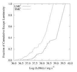
Figure 21.— The cumulative fractional $L_{\rm esc}$ as a function of $\log~{}\mbox{$L$}$ for the LMC (solid line) and SMC (dashed line).

Table 4Global radiative transfer properties of nebular populations

	LMC			SMC
	$\log\mbox{$L$}^{a}$	$\log\mbox{$L_{\rm esc}$}\ ^{b}$	$\langle f_{\rm esc}\rangle$ b	$\log\mbox{$L$}^{a}$	$\log\mbox{$L_{\rm esc}$}\ ^{b}$	$\langle f_{\rm esc}\rangle$ b
Indeterminate (class 0)	39.3	$\cdots$	$\cdots$	36.6	$\cdots$	$\cdots$
Opt Thick (class 1)	39.4	$\cdots$	0.0	38.9	$\cdots$	0.0
Blister (class 2)	39.5	39.1	0.3	38.7	38.4	0.3
Opt Thin (class 3)	39.9	40.0	0.6	39.1	39.2	0.6
Classes $1+2+3$	40.2	40.1	0.42	39.4	39.2	0.40
Kennicutt et al. (1995)c	40.2	40.0	0.35	39.5	39.3	0.41

Note. —

^aColumns 2 and 5 give the sum of the observed $L$.

^b$L_{\rm esc}$ and $\langle f_{\rm esc}\rangle$ are lower limits.

^c$L_{\rm esc}$ from Kennicutt et al. (1995) corresponds to their measured DIG luminosity, $L_{\rm DIG}$.

5.4. Ionizing the WIM

Now, we confront an important question: Can ionizing radiation escaping from optically thin star-forming regions explain the luminosity of the WIM? Previous studies estimated that $\sim$40% of the WIM (or DIG) ionization is due to isolated field stars, and optically thin Hii regions powered by clusters contribute the remaining 60% (e.g. Oey et al. 2004; Hoopes & Walterbos 2000; Oey & Kennicutt 1997; Miller & Cox 1993). From Table 4, we find that $\langle f_{\rm esc}\rangle$ and $L_{\rm esc}$ from the Hii regions alone is enough to balance the observed LMC DIG recombination rate observed by Kennicutt et al. (1995), and that Hii regions account for 84% of the DIG luminosity in the SMC. Including photometric errors, the DIG of both galaxies can be powered by optically thin radiation from Hii regions alone. This is not at odds with the previous results when we consider that not all field stars are sitting naked in the DIG. Many are ionizing discrete nebulae, so that simply adding the ionizing luminosities of all field stars to $L_{\rm esc}$ will overestimate its value.

We have a unique opportunity to examine this quantitatively in the SMC: the RIOTS4 survey of Oey & Lamb (2011) is the only complete survey to target field massive stars in an external galaxy, and it includes 115 spectroscopically confirmed field O stars from the Oey et al. (2004) sample of field OB stars. Of these SMC field O stars, 60 show no associated nebular emission. Using $Q(\rm H^{0})$ from Martins et al. (2005) to convert the stellar spectral types from Oey & Lamb (2011), the total ionizing flux from these is equivalent to 12% of the DIG ionization rate. There are an additional 27 stars whose location inside nebulae is ambiguous. If we assume their ionizing luminosity also streams into the DIG, field O stars produce a total ionization rate equivalent to 23% of the DIG. If we further assume no ionizing radiation escapes the galaxy, then the DIG emission measured by Kennicutt et al. (1995) reflects the combined ionizing radiation from field stars and from optically thin Hii regions, with 77–88% of the ionizing radiation originating from Hii regions. Using equation 4, an SMC aggregate $\mbox{$\langle f_{\rm esc}\rangle$}\sim 0.38-0.41$, instead of 0.40 (Table 4), would result in Hii regions producing 77–88% of the DIG luminosity in Table 4, which is within our $f_{\rm{esc}}$ uncertainty caused by photometry.

5.5. Galactic escape fractions from the Magellanic Clouds

With ample evidence of the great distances that ionizing radiation travels from massive star forming regions, we can make an initial quantitative estimate of $f_{\rm{esc,gal}}$, the galactic escape fraction, by comparing the aggregate escape luminosities from equation 4 to the DIG luminosity $L_{\rm DIG}$, where

$$\mbox{$f_{\rm{esc,gal}}$}=(\mbox{$L$}_{\rm esc}-\mbox{$L$}_{\rm DIG})/\mbox{$L$}_{\rm tot}\quad.$$ (6)

The quantities needed to calculate $f_{\rm{esc,gal}}$ are listed in Table 4, where $\mbox{$L$}_{\rm tot}$ is the sum of observed $L$ and $L_{\rm esc}$, as before. We see that in the SMC, $f_{\rm{esc,gal}}$$=0$. However, as discussed above, this neglects the contribution from a known population of massive field stars. As calculated in §5.4, the ionizing radiation from truly isolated stars in the SMC is 12% – 23% of the DIG luminosity since about half of these field stars reside in Hii regions. In the SMC, this yields a lower limit to $f_{\rm{esc,gal}}$ of 4% – 9%. For the LMC, Table 4 shows that the ionizing luminosity escaping Hii regions is also about the same as the value needed to explain the LMC DIG, without accounting for an unknown population of field O-stars. It is reasonable to assume that the field star ionizing luminosity relative to Hii region $L_{\rm tot}$ is similar (Oey et al. 2004) in the LMC and SMC (0.05 – 0.11). From Table 4 and equation 4 we find a lower limit to $f_{\rm{esc,gal}}$ in the LMC is 11–17%.

It is important to bear in mind that our constraints on nebular $\langle f_{\rm esc}\rangle$ technically are lower limits, as stressed in §2. The ranges in galactic escape fraction quoted above only reflect the uncertainties in the field star population. Thus it is possible that $f_{\rm{esc,gal}}$ may be underestimated in one or both of the galaxies; the crude estimates in Table 4 preclude any conclusive results. Future work is needed to quantitatively improve these constraints. Further efforts may be directed at obtaining more definitive ionization-parameter mapping by adding imaging in more ions, or modeling diagnostic emission lines in filaments ionized by distant sources like those for 30 Doradus and N66, which can constrain the ionizing photon flux and SED of these dominant objects.

6. Conclusions

We have demonstrated the power of spatially resolved, ionization-parameter mapping to quantitatively probe the optical depth of Hii regions to the Lyman continuum. Our Cloudy photoionization simulations show that spatially resolved emission-line ratio mapping reveals the presence or absence of ionization stratification that diagnoses the optical depth of photoionized regions. The technique also constrains the optical depth in the line of sight. We show that ionization-parameter mapping in only [S$\rm II$] and [O$\rm III$] is a powerful and productive technique when studying global nebular properties. Although there is a degeneracy between optically thin and weakly ionized regions when using only two radially varying ions, the technique works well in the aggregrate, and the degeneracy is resolved with observations of three sensitive ions. It may be possible to develop similar methods using emission from PAHs, which are easily destroyed in ionized gas, and enhanced by non-ionizing UV light in ionization fronts.

Our application of ionization-parameter mapping uses the [S$\rm II$], [O$\rm III$], and H$\alpha$ data of the LMC and SMC from the MCELS survey. First, we used [S$\rm II$]/[O$\rm III$] ratio maps to define new boundaries for photoionized Hii regions. The [S$\rm II$]/[O$\rm III$] maps reveal the nebular ionization structure, thereby allowing us to isolate the emission from individual photoionized Hii regions, even if they are overlapping and/or embedded in large complexes or bright DIG. We used these data, together with the H$\alpha$ surface brightness, to define the boundaries of 401 Hii regions in the LMC and 214 in the SMC. The resulting Hii region luminosity functions are consistent with those published for these same galaxies (Kennicutt et al., 1989), indicating that the simpler, H$\alpha$-only boundary criteria do result in statistical properties that are similar to those for objects defined by our more physically motivated criteria.

Based on their observed ionization structures, the optical depths of the individual Hii regions were crudely divided into optically thin, optically thick, and blister classes. Based on our models, we assign $\mbox{$f_{\rm{esc}}$}=0.6$ for the population of optically thin regions, 0.3 for blisters, and 0.0 for the optically thick objects. These estimates agree within 23% with more direct measurements of the optical depth for a sample of objects with known spectral classifications for the ionizing stars.

These rough optical depth classes already yield fundamental new insights into the quantitative radiation transfer of the nebular population and DIG ionization in these galaxies. We find that the frequency of optically thin nebulae is 40% in the LMC and 33% in the SMC. The luminosity distributions reveal that the median luminosity of optically thin nebulae is significantly brighter than for those which are optically thick, by a factor of 2 – 5. More importantly, the frequency of optically thin nebulae increases with $L$, such that above $\log~{}\mbox{$L$}/(\mbox{${\rm erg\ s^{-1}}$})=37.0$, Hii regions in both galaxies are dominated by optically thin objects. Due to their high luminosity and significant $f_{\rm{esc}}$, these objects also dominate the total ionizing radiation leaking into the DIG. It will be important to determine whether all star-forming galaxies show a similar luminosity threshold for the dominance of optically thin objects.

We also see a correlation in the frequency of optically thick regions and Hi column density, with the median $N{\rm(HI)}$ of optically thick nebulae 1.5 and 1.2 times higher than those of optically thin ones in in the LMC and SMC, respectively. In contrast, the median $N{\rm(HI)}$ of all objects measured in the SMC is 2.4 times higher than in the LMC, probably owing to projection effects. It is surprising that despite major differences in the character of the ambient neutral ISM outside of Hii regions, the quantitative properties of the LyC radiative transfer within the nebulae are remarkably similar between the two galaxies. This brings us to an important conclusion: the large-scale fate of ionizing radiation emitted by O-stars in the LMC and SMC may be determined by the external, neutral Hi environment, which in the SMC appears more efficient at trapping radiation once it escapes optically thin Hii regions (e.g. the southwest region of the SMC).

Optically thin nebulae are sufficiently luminous to maintain the ionization of the DIG in both galaxies, as measured by Kennicutt et al. (1995). We also consider the global escape fraction of ionizing radiation from these galaxies into the IGM. We find evidence that luminous, optically thin Hii regions near the outer edges of both galaxies may produce ionizing radiation that escapes into the interstellar environment. This is evidenced by the kpc-scale path lengths traveled by ionizing photons from these massive Hii regions, shown by the existence of extended [O$\rm III$] halos opening toward the IGM.

We find the combined, luminosity-weighted, LyC escape fractions from all Hii regions to be at least 0.42 and 0.40 in the LMC and SMC, respectively. The corresponding escape luminosities are at least $\log$ $L_{\rm esc}$/$({\rm erg\ s^{-1}})=40.1$ and 39.2 in the LMC and SMC, respectively. Considering the existence of field O stars with no nebulae, the implied total available LyC luminosity is greater than needed to explain the DIG emission in both galaxies. These are still crude estimates, but an excess implies that a fraction of the ionizing radiation produced leaves the galaxy and may enter the IGM. We currently estimate lower limits to the galactic escape fractions of $\mbox{$f_{\rm{esc,gal}}$}=$ 4 – 9% in the SMC, and 11 – 17% in the LMC. These values are consistent with $f_{\rm{esc,gal}}$ $\sim$10% – 20%, as required for cosmic reionization to be driven by star forming galaxies at high redshift (Sokasian et al., 2003). These estimates for $f_{\rm{esc,gal}}$ would increase when accounting for lower optical depth due to absence of dust and metals at high redshift.

Appendix A A. SurfBright: Modeling surface brightness using Cloudy

The comparison of 1-D photoionization models to observations is most commonly done with spatially integrated emission-line fluxes. This approach is used because a direct comparison to the observed surface-brightness profile of a nebula involves the convolution of nebular geometry with a changing volume emissivity. While computing predicted surface brightnesses is more difficult, it does provide important, additional constraints on a model.

We developed the Perl routine SurfBright, which calculates the projected, 2-D surface brightness of isotropically emitted emission lines in a nebula. This code uses the results of 1-D Cloudy simulations and a user specified 3-D geometry. The code works in Cartesian coordinates relative to the nebula with z parallel to the line of sight from observer to object. This geometry is defined at each $x,y$ coordinate (projected on the sky) by the minimum and maximum radial distance of the cloud along the line of sight $z_{min}(x,y),\ z_{max}(x,y)$. A specified physical geometry allows for the prediction of absolute nebular surface brightness. With the object-observer distance and 2-D spatial resolution $\Delta x$ and $\Delta y$, observations can be simulated for any arcsec, pc or cm pixel scale. Line strength is given in units of surface brightness, which is is independent of the distance between observer and object, for resolved nebulae.

A schematic of a Cloudy simulation is shown in Figure 22$a$. The uneven spacing of shells around the ionizing star reflects the individual zones calculated within a Cloudy simulation, which are set by changes in the physical conditions of the gas as a function of depth. The Cloudy simulation calculates the isotropic volume emissivity $\epsilon$ of each emission line in each radial zone. At each $x,y$ coordinate projected in the plane perpendicular to the line of sight $z$, SurfBright calculates the observed surface brightness in the $i^{th}$ emission line from all Cloudy shells according to,

$$S_{i}=\sum_{j}dl_{j}(x,y)\times\epsilon_{i}(x,y,z)/4\pi\times 2.3504\times 10^{-11}\ \rm\mbox{${\rm erg\ s^{-1}}$}cm^{-2}~{}arcsec^{-2}\quad,$$ (A1)

where $dl_{j}$ is the path length along the line of sight ($z$-axis) through shell $j$ at the projected position $x,y$; and $\epsilon_{i}$ are the local volume emissivities taken from the 1-D Cloudy simulation where the 1-D radius $r$ in the model is equal to the magnitude of the radius of the geometrically defined cloud r($x,y,z$).

Our method of integrating the emission along the line of sight, from the far to near side of the Hii region, also allows us to include the effects of internal extinction, which is important for nebulae with a high observed column density, such as photodissociation regions and molecular clouds. (Pellegrini et al., 2009). Computationally, we first determine the line flux entering a given shell, which is added to the diffuse flux in that shell. The sum is locally extinguished by the internal extinction in a shell calculated by Cloudy scaled by $dl/dr$, where $dr$ is the shell thickness. This determines the flux entering the next shell along a line of sight toward the observer.

SurfBright currently includes generic geometrical configurations for planar slabs and simple spheres. The orientation, length and inclination of the slab are free parameters. Whole and truncated spheres as in Figure 22$b$ are also possible. Future support will include completely arbitrary geometric configurations. Currently the code uses only one Cloudy model to determine the emissivity as a function of r. Later we will also add the ability to first define a geometry with initial density parameters and calculate the needed Cloudy simulations from the specified geometry when predicting observations. This will make it possible to accurately model the emission from complex, irregular nebulae with different ionization parameters.

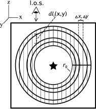
(a) Sphere

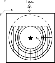
(b) Truncated Sphere

Figure 22.— Schematic representation showing the conversion from a 1-D Cloudy simulation into a 2-D SurfBright surface brightness model. Vertical lines represent lines of sight along the $z$-axis through the nebula at various projected $x,y$ positions. The shell structure results from the 1-D Cloudy calculation. Panel ($a$) shows spherically symmetric geometry, and panel ($b$) shows an object with truncated spherical geometry.

Appendix B B. New LMC and SMC Hii Region Catalogs

Tables LABEL:tab:LMCObjs and LABEL:tab:SMCObjs present our new Hii region catalogs, with the nebular boundaries defined by ionization-parameter mapping as described in §3.1. Some objects are defined within the boundaries of larger, background objects, and their flux is not included in the luminosity for the larger objects. The Hii regions are classified by optical depth as described in §4, into types 0 – 4, corresponding to (0) indeterminate, (1) optically thick, (2) blister, (3) optically thin, and (4) shocked. The object ID’s are listed in columns 1 and 2, with our new designations in the former and identifications from existing catalogs in the latter. We designate new, independent substructures within a previously catalogued object by appending numbers, for example, DEM L173-1 and DEM L173-2. The object coordinates are listed in columns 3 and 4; optical depth classifications are given in column 5. Columns 6 and 7 respectively give the average $N{\rm(HI)}$ measured in the line of sight within the nebular aperture, and the H$\alpha$ luminosity $L$.

In Figures 23 and 24, we present representative images in H$\alpha$ and [S$\rm II$]/[O$\rm III$], of five objects in each galaxy. Each image is centered on the coordinates listed in Tables LABEL:tab:LMCObjs and LABEL:tab:SMCObjs. The images show the aperture used to measure the H$\alpha$ flux, as well as a scale bar in both arcsec and pc. When shown with dashed lines, apertures have been enlarged to reveal underlying structure. There are two labels in each image: our MCELS catalog ID in the upper left, and, centered above the object, an alternate catalog ID, unless none exists. The complete set of images can be found in the online edition of this article.

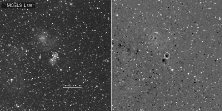
(a) MCELS-L001

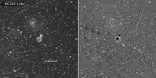
(b) MCELS-L002

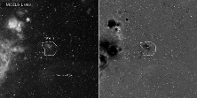
(c) MCELS-L003

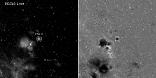
(d) MCELS-L004

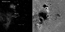
(e) MCELS-L005

Figure 23.— 5 LMC Hii regions from the MCELS catalog in H$\alpha$(left) and [S$\rm II$]/[O$\rm III$](right).

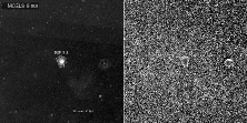
(a) MCELS-S 001

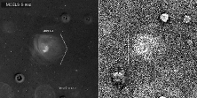
(b) MCELS-S 002

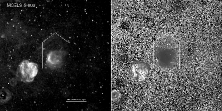
(c) MCELS-S 003

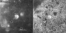
(d) MCELS-S 004

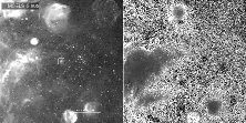
(e) MCELS-S 005

Figure 24.— 5 SMC Hii regions from the MCELS-S catalog in H$\alpha$ and [S$\rm II$]/[O$\rm III$].

Table 5REVISED - MCELS LMC HII Region Catalog - REVISED

Object ID	Other IDa	RA (J2000)	Dec	Typeb	$N$(HI)	$L$(H$\alpha$)
		h:m:s	d:m:s		$10^{21}cm^{-2}$	${\rm erg\ s^{-1}}$
MCELS-L1	$\cdots$	04:44:59.7	-69:03:22	2	1.75	35.12
MCELS-L2	$\cdots$	04:45:04.8	-69:04:25	2	1.90	35.27
MCELS-L3	DEM L1	04:47:19.5	-69:18:27	2	1.89	36.41
MCELS-L4	DEM L2	04:48:53.7	-69:09:38	1	3.24	36.51
MCELS-L5	DEM L6	04:49:06.8	-69:20:26	1	2.71	36.53
MCELS-L6	DEM L3	04:49:07.4	-68:24:17	1	2.34	36.55
MCELS-L7	DEM L4	04:49:11.3	-69:16:08	0	3.00	36.35
MCELS-L8	DEM L4	04:49:18.4	-69:13:54	1	3.57	35.91
MCELS-L9	DEM L4	04:49:18.7	-69:13:20	1	3.52	35.70
MCELS-L10	DEM L5	04:49:24.4	-69:07:37	3	3.24	35.90
MCELS-L11	DEM L4	04:49:25.2	-69:15:24	1	3.29	35.85c
MCELS-L12	DEM L4	04:49:25.9	-69:12:00	3	3.08	37.08
MCELS-L13	DEM L4	04:49:30.7	-69:13:35	3	3.49	36.66c
MCELS-L14	DEM L4	04:49:44.4	-69:12:55	1	3.54	36.02
MCELS-L15	DEM L6	04:49:49.2	-69:20:03	3	3.31	37.46
MCELS-L16	DEM L4	04:49:51.0	-69:11:44	3	2.97	37.36d
MCELS-L17	DEM L4	04:50:02.4	-69:13:23	1	2.94	35.80d
MCELS-L18	DEM L4	04:50:05.9	-69:12:05	1	2.98	35.81c
MCELS-L19	DEM L7	04:50:08.0	-67:42:10	0	1.35	37.32
MCELS-L20	DEM L6	04:50:37.8	-69:25:28	3	2.75	37.64
MCELS-L21	$\cdots$	04:51:32.2	-68:24:24	3	1.53	35.84
MCELS-L22	DEM L8a	04:51:44.2	-66:55:14	1	3.16	36.29
MCELS-L23	DEM L10a	04:51:47.5	-69:23:10	1	1.73	36.71
MCELS-L24	DEM L10a	04:51:49.0	-69:24:25	3	2.00	37.16
MCELS-L25	DEM L10a	04:51:52.8	-69:23:29	1	2.22	37.16
MCELS-L26	DEM L17	04:51:54.0	-70:47:01	0	1.45	36.63
MCELS-L27	DEM L8b	04:52:07.4	-66:55:31	3	3.15	37.41
MCELS-L28	DEM L8c	04:52:11.7	-66:54:29	1	3.87	36.63
MCELS-L29	DEM L10b	04:52:13.0	-69:20:16	2	3.04	37.69
MCELS-L30	BSDL139	04:52:17.5	-70:36:29	0	1.51	35.56
MCELS-L31	DEM L9	04:52:19.4	-68:24:39	0	1.59	36.30
MCELS-L32	$\cdots$	04:52:23.3	-66:55:16	1	3.02	35.62
MCELS-L33	DEM L10b	04:52:26.5	-69:21:45	1	2.99	36.99
MCELS-L34	DEM L11	04:52:34.4	-67:17:23	1	1.62	37.29
MCELS-L35	$\cdots$	04:52:35.0	-66:55:41	1	2.45	35.82
MCELS-L36	DEM L15	04:52:46.5	-69:12:54	1	2.73	37.12
MCELS-L37	DEM L14	04:52:47.1	-68:54:40	0	1.90	36.37
MCELS-L38	DEM L10b	04:52:59.5	-69:23:30	3	2.18	37.20
MCELS-L39	DEM L13	04:53:06.3	-68:02:38	2	1.57	37.60
MCELS-L40	DEM L15	04:53:07.1	-69:14:11	3	3.21	36.64
MCELS-L41	DEM L12	04:53:21.0	-66:56:19	4	1.72	37.16
MCELS-L42	DEM L21	04:53:26.0	-70:36:00	3	1.07	36.85
MCELS-L43	DEM L20	04:53:30.6	-67:23:22	1	1.34	36.23
MCELS-L44	DEM L18	04:53:33.3	-67:03:30	3	1.96	36.26
MCELS-L45	DEM L19	04:53:35.5	-67:14:09	3	1.17	36.79
MCELS-L46	DEM L16	04:53:38.8	-68:49:00	0	1.28	36.67
MCELS-L47	DEM L22	04:53:57.5	-69:10:28	1	2.80	36.64
MCELS-L48	DEM L25	04:53:58.9	-70:00:53	2	0.63	37.29
MCELS-L49	DEM L22	04:54:03.3	-69:12:08	2	2.56	37.64
MCELS-L50	DEM L27	04:54:11.0	-66:54:01	0	1.51	36.64
MCELS-L51	DEM L29a	04:54:12.3	-66:45:45	0	2.09	35.34
MCELS-L52	DEM L26	04:54:13.4	-68:21:52	1	1.76	37.08
MCELS-L53	DEM L23	04:54:24.4	-69:29:43	0	3.10	35.87
MCELS-L54	DEM L22	04:54:25.2	-69:10:57	1	2.22	36.87
MCELS-L55	DEM L22	04:54:27.6	-69:09:37	1	2.32	37.19
MCELS-L56	DEM L29b	04:54:27.7	-66:44:35	2	1.49	35.36
MCELS-L57	DEM L30	04:55:03.0	-67:15:53	0	1.74	36.44
MCELS-L58	DEM L31	04:55:10.9	-67:11:32	3	1.11	37.77
MCELS-L59	DEM L22	04:55:17.7	-69:11:45	2	2.05	37.26
MCELS-L60	DEM L24	04:55:25.6	-69:16:06	1	0.99	36.06
MCELS-L61	DEM L32	04:55:34.5	-68:25:39	1	2.56	36.58
MCELS-L62	DEM L33	04:55:40.8	-68:38:43	0	1.70	37.08
MCELS-L63	DEM L35	04:55:58.4	-65:57:50	2	1.78	36.73
MCELS-L64	DEM L36	04:56:33.5	-69:29:04	0	1.07	37.55
MCELS-L65	DEM L34	04:56:34.3	-66:26:52	2	2.99	39.01
MCELS-L66	DEM L37	04:56:58.4	-69:12:45	1	1.91	36.61
MCELS-L67	DEM L38	04:57:05.8	-68:44:58	2	1.87	37.36
MCELS-L68	DEM L40	04:57:32.7	-67:39:10	0	1.64	36.36
MCELS-L69	$\cdots$	04:57:44.0	-66:15:31	1	4.68	36.11
MCELS-L70	DEM L41	04:58:10.3	-66:21:34	1	4.28	37.47
MCELS-L71	DEM L39	04:58:29.7	-68:27:02	2	1.12	38.12
MCELS-L72	DEM L42	04:58:48.4	-66:11:38	1	2.84	37.38
MCELS-L73	N12A	04:58:57.3	-66:13:58	1	3.11	35.98
MCELS-L74	DEM L43+48	04:58:58.8	-65:40:28	1	0.93	38.25
MCELS-L75	DEM L44	04:59:12.0	-66:16:03	1	3.07	36.24
MCELS-L76	DEM L50	04:59:45.5	-70:09:45	4	1.28	37.37
MCELS-L77	DEM L45	04:59:57.2	-67:56:48	3	0.98	37.28
MCELS-L78	DEM L51	05:00:00.3	-70:03:30	1	0.93	36.05
MCELS-L79	DEM L46	05:00:06.6	-66:15:39	1	2.23	36.91
MCELS-L80	DEM L47	05:00:10.3	-66:05:37	1	3.29	36.60
MCELS-L81	DEM L49	05:00:52.5	-66:23:16	0	2.15	35.94
MCELS-L82	DEM L52	05:01:48.0	-68:12:41	0	1.63	36.00
MCELS-L83	DEM L55	05:01:50.5	-70:38:37	0	0.62	37.03
MCELS-L84	DEM L53	05:01:52.5	-70:04:48	0	0.63	36.27
MCELS-L85	DEM L54	05:02:07.0	-69:34:02	0	0.72	35.53
MCELS-L86	BSDL453	05:02:09.2	-66:40:18	2	1.29	36.30
MCELS-L87	DEM L60	05:02:12.7	-69:03:38	0	2.54	36.46
MCELS-L88	DEM L57	05:02:48.6	-67:00:01	0	1.82	36.56
MCELS-L89	DEM L61	05:03:13.2	-65:57:24	0	2.38	36.88
MCELS-L90	DEM L58	05:03:15.6	-68:27:07	0	1.37	36.20
MCELS-L91	DEM L56	05:03:22.8	-66:42:02	0	1.34	36.42
MCELS-L92	DEM L59	05:04:20.1	-67:18:35	2	2.27	37.45
MCELS-L93	DEM L63	05:04:23.5	-70:44:07	1	1.37	37.18
MCELS-L94	DEM L62	05:04:25.2	-69:03:33	0	1.86	37.23
MCELS-L95	DEM L64a	05:04:31.4	-70:54:06	1	1.78	36.22
MCELS-L96	DEM L64b	05:04:38.9	-70:54:43	1	2.03	36.75
MCELS-L97	DEM L68	05:04:39.3	-70:10:32	1	1.34	35.93
MCELS-L98	DEM L68	05:04:47.9	-70:05:39	1	2.16	35.25
MCELS-L99	DEM L65	05:04:48.8	-67:33:18	2	1.94	36.84
MCELS-L100	DEM L67	05:04:55.1	-70:07:41	1	1.91	36.38
MCELS-L101	DEM L66	05:05:00.2	-68:03:41	3	1.58	37.56
MCELS-L102	DEM L68	05:05:06.7	-70:06:24	3	1.29	37.51d
MCELS-L103	DEM L70	05:05:16.7	-68:05:41	3	1.56	36.94
MCELS-L104	DEM L69	05:05:16.9	-66:55:15	1	2.01	36.68
MCELS-L105	DEM L71	05:05:41.0	-67:52:49	0	1.63	35.58
MCELS-L106	DEM L72	05:06:05.0	-65:41:29	3	1.55	36.46
MCELS-L107	DEM L73	05:06:12.1	-68:07:28	1	2.33	37.48
MCELS-L108	DEM L76	05:06:45.3	-68:26:34	3	1.52	37.51
MCELS-L109	DEM L74	05:06:46.3	-68:09:54	1	2.77	36.69
MCELS-L110	DEM L75	05:06:47.4	-70:44:44	0	0.93	37.09
MCELS-L111	DEM L77	05:06:50.1	-66:54:56	0	1.24	36.65
MCELS-L112	DEM L78	05:06:59.9	-67:56:46	0	1.17	35.28
MCELS-L113	DEM L80	05:07:19.1	-70:27:02	0	0.93	37.42
MCELS-L114	DEM L79	05:07:21.5	-68:32:05	1	2.12	36.76
MCELS-L115	DEM L81	05:07:37.5	-71:10:32	0	0.91	36.10
MCELS-L116	DEM L83	05:07:39.3	-71:01:30	0	0.94	35.76
MCELS-L117	DEM L84	05:08:42.6	-68:45:52	4	1.83	37.86
MCELS-L118	DEM L85	05:09:24.0	-68:45:44	1	3.14	36.76
MCELS-L119	DEM L86	05:09:34.3	-68:53:45	3	2.55	38.13
MCELS-L120	DEM L91	05:09:38.1	-71:26:22	0	1.05	36.29
MCELS-L121	DEM L89	05:09:39.5	-67:55:14	3	1.86	37.45
MCELS-L122	DEM L88	05:09:53.0	-68:29:11	1	2.37	37.10
MCELS-L123	DEM L90	05:10:23.0	-67:09:27	0	2.06	36.32
MCELS-L124	DEM L92	05:10:30.3	-69:25:56	0	1.38	36.56
MCELS-L125	DEM L93	05:10:43.5	-67:04:50	1	2.03	36.05
MCELS-L126	DEM L95	05:10:54.3	-69:03:09	0	2.33	35.57
MCELS-L127	DEM L94	05:10:59.4	-67:07:34	1	1.66	36.18
MCELS-L128	DEM L96	05:11:23.6	-69:03:54	1	2.71	35.76
MCELS-L129	DEM L97	05:12:07.7	-67:06:54	0	2.88	36.96
MCELS-L130	DEM L100	05:12:08.2	-70:28:43	1	2.17	35.14
MCELS-L131	DEM L100	05:12:15.0	-70:28:05	1	2.03	35.91
MCELS-L132	DEM L100	05:12:21.9	-70:27:33	1	1.87	35.33
MCELS-L133	DEM L98	05:12:24.5	-67:15:40	0	2.41	36.37
MCELS-L134	DEM L101	05:12:28.4	-70:24:52	1	2.50	35.70
MCELS-L135	DEM L101	05:12:30.2	-70:24:22	3	2.61	36.52
MCELS-L136	DEM L101	05:12:30.4	-70:25:22	1	2.22	34.99
MCELS-L137	DEM L102	05:12:44.2	-70:22:02	2	2.22	36.14
MCELS-L138	DEM L99	05:12:48.7	-67:02:18	1	2.31	36.29
MCELS-L139	DEM L103	05:13:07.1	-69:01:56	0	2.27	36.64
MCELS-L140	DEM L104	05:13:10.4	-69:22:35	1	2.81	37.26
MCELS-L141	N30D	05:13:16.3	-67:28:24	1	2.94	36.17
MCELS-L142	DEM L111	05:13:18.7	-71:22:05	0	1.25	35.98
MCELS-L143	DEM L104	05:13:19.0	-69:21:26	1	2.76	37.45
MCELS-L144	DEM L104	05:13:21.4	-69:22:38	1	2.60	36.68
MCELS-L145	DEM L109	05:13:25.4	-69:10:55	0	2.15	36.29
MCELS-L146	DEM L108	05:13:34.9	-69:17:06	2	2.48	37.76
MCELS-L147	DEM L104	05:13:40.5	-69:22:30	2	1.60	37.19
MCELS-L148	DEM L105	05:13:43.4	-67:22:43	2	1.66	37.53
MCELS-L149	DEM L104	05:13:48.5	-69:23:15	1	1.77	36.81
MCELS-L150	DEM L106	05:13:53.1	-67:27:05	2	2.93	37.56
MCELS-L151	DEM L110	05:14:01.8	-69:31:55	2	1.30	37.37
MCELS-L152	DEM L107+115	05:14:06.0	-67:09:02	3	1.75	37.52
MCELS-L153	DEM L114	05:14:08.2	-70:07:43	0	1.68	35.54
MCELS-L154	DEM L112	05:14:34.4	-67:34:03	0	2.52	36.78
MCELS-L155	DEM L119	05:14:53.1	-71:37:09	3	1.21	36.83
MCELS-L156	DEM L113	05:14:53.8	-69:25:58	0	1.60	37.44
MCELS-L157	DEM L116	05:15:07.2	-66:28:06	1	1.07	36.29
MCELS-L158	DEM L120	05:15:20.5	-69:43:30	0	1.36	36.04
MCELS-L159	DEM L117	05:15:34.1	-67:20:35	0	1.77	35.73
MCELS-L160	DEM L118	05:15:45.7	-66:42:49	0	1.36	36.17
MCELS-L161	DEM L124	05:16:53.1	-69:53:01	0	2.02	36.21
MCELS-L162	DEM L121	05:16:53.4	-67:19:51	1	2.20	36.90
MCELS-L163	$\cdots$	05:17:02.9	-66:00:55	2	1.07	35.84
MCELS-L164	DEM L122	05:17:06.2	-68:52:35	0	3.39	35.05
MCELS-L165	DEM L131	05:17:39.1	-71:15:32	2	1.72	37.35
MCELS-L166	DEM L130	05:17:44.5	-69:24:00	0	2.34	36.96
MCELS-L167	DEM L128	05:17:46.0	-68:47:04	1	3.54	36.13
MCELS-L168	DEM L129	05:17:48.0	-67:54:05	2	1.83	36.19
MCELS-L169	DEM L127	05:17:49.0	-67:20:58	2	1.28	37.01
MCELS-L170	DEM L125	05:17:51.0	-66:01:17	1	1.45	37.11
MCELS-L171	DEM L123+132	05:17:59.7	-69:11:01	2	2.23	38.54
MCELS-L172	DEM L126	05:18:16.6	-65:57:41	0	1.67	36.49
MCELS-L173	DEM L134	05:18:27.4	-69:39:55	1	2.81	36.85
MCELS-L174	$\cdots$	05:18:40.6	-67:05:21	3	1.29	36.32
MCELS-L175	DEM L134	05:18:43.7	-69:39:15	1	2.14	36.83
MCELS-L176	DEM L134+133	05:19:16.4	-69:38:43	2	1.47	38.09
MCELS-L177	DEM L134	05:19:35.8	-69:38:47	3	2.25	36.32
MCELS-L178	DEM L135	05:19:48.3	-65:53:53	0	0.91	37.38
MCELS-L179	DEM L139	05:20:19.4	-66:28:54	0	1.40	35.37
MCELS-L180	DEM L136	05:20:22.1	-66:53:42	2	1.61	36.89
MCELS-L181	DEM L141	05:20:30.6	-68:01:02	1	3.59	36.14
MCELS-L182	DEM L138	05:20:34.0	-66:46:38	2	2.02	37.03
MCELS-L183	$\cdots$	05:20:40.3	-66:48:46	0	2.40	35.10
MCELS-L184	DEM L137	05:20:48.7	-65:27:25	3	0.77	37.64
MCELS-L185	DEM L146	05:20:54.5	-71:43:17	0	1.99	35.66
MCELS-L186	$\cdots$	05:21:04.9	-71:41:43	0	1.95	35.02
MCELS-L187	$\cdots$	05:21:17.4	-66:47:14	0	2.31	35.37
MCELS-L188	DEM L145	05:21:19.3	-69:40:50	1	2.42	36.71
MCELS-L189	DEM L147	05:21:26.3	-69:56:50	0	1.81	35.91
MCELS-L190	DEM L143	05:21:26.9	-68:52:04	0	1.87	36.86
MCELS-L191	DEM L144	05:21:31.1	-68:10:48	2	3.94	35.94
MCELS-L192	DEM L149	05:21:34.6	-69:40:27	1	3.01	37.15
MCELS-L193	DEM L150	05:21:36.6	-67:46:34	1	2.90	36.24
MCELS-L194	DEM L140	05:21:37.1	-67:54:49	1	3.06	37.46
MCELS-L195	DEM L148	05:21:37.3	-69:59:37	0	2.10	36.40
MCELS-L196	DEM L151a	05:21:46.8	-67:53:42	0	4.44	36.80
MCELS-L197	DEM L153	05:21:49.7	-69:41:09	1	3.15	35.85
MCELS-L198	DEM L151	05:21:49.9	-67:51:46	0	3.01	37.39
MCELS-L199	DEM L142	05:21:53.9	-65:43:49	0	0.97	37.18
MCELS-L200	DEM L154	05:22:00.9	-65:58:22	2	0.92	37.57
MCELS-L201	DEM L152	05:22:06.9	-67:56:46	3	3.97	38.19
MCELS-L202	DEM L164	05:22:13.1	-71:26:10	2	1.25	37.59
MCELS-L203	DEM L157	05:22:16.3	-68:38:58	1	1.68	36.61
MCELS-L204	DEM L158	05:22:19.4	-68:04:26	1	4.89	36.64
MCELS-L205	DEM L155	05:22:25.5	-65:44:46	0	1.24	37.32d
MCELS-L206	DEM L156	05:22:26.9	-67:53:41	1	4.23	37.39
MCELS-L207	DEM L165	05:22:27.8	-71:35:51	1	1.88	37.57
MCELS-L208	DEM L158	05:22:29.9	-68:04:52	1	4.45	35.93
MCELS-L209	DEM L163	05:22:32.3	-70:08:45	2	1.10	36.50
MCELS-L210	DEM L159	05:22:36.2	-68:08:32	1	4.68	36.56
MCELS-L211	$\cdots$	05:22:37.0	-66:38:52	2	2.70	35.46
MCELS-L212	DEM L160	05:22:45.2	-68:04:00	1	4.51	37.89
MCELS-L213	DEM L161	05:22:48.0	-66:41:06	1	3.15	36.38
MCELS-L214	DEM L168	05:22:52.7	-69:50:58	0	2.20	36.40
MCELS-L215	DEM L155a	05:22:53.6	-65:43:03	1	1.54	36.88
MCELS-L216	DEM L166a	05:23:06.0	-68:00:17	1	3.74	36.28
MCELS-L217	DEM L162	05:23:06.8	-66:22:32	1	1.97	36.52
MCELS-L218	DEM L166b	05:23:12.5	-68:00:18	1	4.23	36.55
MCELS-L219	DEM L167	05:23:16.5	-67:56:14	1	3.53	36.65
MCELS-L220	DEM L170	05:23:27.4	-68:12:25	0	2.55	36.10
MCELS-L221	DEM L171	05:23:33.5	-69:38:51	0	2.04	36.60
MCELS-L222	DEM L169	05:23:39.5	-68:00:43	1	3.51	36.26
MCELS-L223	DEM L172	05:23:40.6	-69:37:01	2	1.00	36.91
MCELS-L224	DEM L173	05:23:50.8	-69:41:26	0	2.66	36.26
MCELS-L225	DEM L176a	05:24:03.0	-68:56:21	0	2.47	35.34
MCELS-L226	DEM L173	05:24:04.1	-69:40:18	1	3.19	36.08
MCELS-L227	DEM L173	05:24:07.0	-69:38:43	1	2.18	36.05
MCELS-L228	DEM L176b	05:24:09.4	-68:55:53	0	2.46	35.24
MCELS-L229	DEM L174	05:24:12.3	-68:30:09	1	2.76	36.31
MCELS-L230	N132B	05:24:17.5	-69:38:56	1	2.09	35.95
MCELS-L231	DEM L174	05:24:22.7	-68:31:34	3	2.21	37.56d
MCELS-L232	DEM L175	05:24:24.1	-66:14:29	2	2.69	37.30
MCELS-L233	DEM L194	05:24:28.2	-71:38:36	0	2.16	36.00
MCELS-L234	DEM L178	05:24:34.2	-69:27:09	0	1.15	36.92
MCELS-L235	DEM L177	05:24:36.9	-69:06:55	0	1.76	38.32
MCELS-L236	DEM L182+184	05:24:38.5	-66:57:13	0	1.51	37.43
MCELS-L237	DEM L179	05:24:39.2	-68:28:47	1	3.24	36.26
MCELS-L238	DEM L180	05:24:58.2	-68:28:41	2	3.01	37.23
MCELS-L239	DEM L175a	05:24:58.5	-66:26:03	3	3.83	37.17
MCELS-L240	DEM L186	05:25:02.4	-69:38:34	3	2.03	36.26
MCELS-L241	DEM L188	05:25:06.1	-71:27:49	2	1.58	35.98
MCELS-L242	DEM L181	05:25:21.7	-66:02:46	2	2.56	37.17
MCELS-L243	DEM L187	05:25:25.4	-69:26:10	0	1.00	36.91
MCELS-L244	DEM L183	05:25:27.4	-66:21:52	1	3.98	36.07
MCELS-L245	DEM L185	05:25:54.5	-65:55:53	0	2.34	35.94
MCELS-L246	DEM L190	05:26:01.3	-66:04:57	4	3.91	37.19
MCELS-L247	DEM L189	05:26:04.1	-66:15:47	0	4.41	37.67
MCELS-L248	DEM L193	05:26:10.0	-67:10:37	3	1.43	37.31
MCELS-L249	DEM L195	05:26:12.7	-66:21:47	0	1.75	37.48
MCELS-L250	DEM L192+201	05:26:13.1	-67:29:56	1	1.90	38.52
MCELS-L251	DEM L196	05:26:13.9	-67:37:13	1	2.27	36.38
MCELS-L252	DEM L196	05:26:20.7	-67:37:55	1	1.86	37.60
MCELS-L253	DEM L189	05:26:23.2	-66:14:31	2	4.40	36.28
MCELS-L254	DEM L197	05:26:28.6	-69:18:58	3	0.78	37.38
MCELS-L255	DEM L196	05:26:28.6	-67:42:01	2	2.07	35.98
MCELS-L256	DEM L198	05:26:32.2	-69:02:04	0	1.20	37.77
MCELS-L257	DEM L196	05:26:37.9	-67:43:28	1	2.58	36.00
MCELS-L258	DEM L199	05:26:42.5	-68:49:34	3	1.18	38.36
MCELS-L259	DEM L202	05:27:10.3	-71:32:06	2	1.99	37.57
MCELS-L260	DEM L208	05:27:17.6	-70:34:46	3	1.01	37.73
MCELS-L261	DEM L206	05:27:26.8	-71:23:28	2	3.09	36.01
MCELS-L262	$\cdots$	05:27:31.3	-67:27:31	0	2.18	37.51
MCELS-L263	DEM L203	05:27:31.4	-68:27:00	0	1.68	38.38
MCELS-L264	DEM L207	05:27:41.6	-71:24:46	1	2.47	36.26
MCELS-L265	DEM L204	05:27:54.2	-65:50:10	4	0.65	36.49
MCELS-L266	DEM L209	05:28:02.2	-69:21:36	0	0.87	37.63
MCELS-L267	DEM L205	05:28:06.2	-67:26:50	2	2.56	37.59
MCELS-L268	BSDL1844	05:28:14.6	-67:23:57	1	2.50	36.67
MCELS-L269	DEM L210	05:28:19.2	-69:01:21	0	1.52	37.96
MCELS-L270	DEM L213	05:28:43.1	-70:20:20	0	1.44	36.44
MCELS-L271	DEM L211	05:28:54.3	-67:43:24	0	1.58	36.57
MCELS-L272	DEM L214	05:29:17.4	-66:57:21	0	0.69	36.95
MCELS-L273	DEM L215	05:29:33.4	-69:48:48	0	1.23	37.26
MCELS-L274	$\cdots$	05:29:52.2	-71:04:33	1	2.17	36.56
MCELS-L275	DEM L216	05:30:09.4	-69:45:09	0	0.91	36.18
MCELS-L276	DEM L218	05:30:33.9	-70:07:59	0	1.41	37.02
MCELS-L277	DEM L221	05:30:34.0	-71:01:21	1	2.02	38.43
MCELS-L278	N206B	05:30:51.2	-71:08:01	1	3.48	36.83
MCELS-L279	DEM L222a	05:30:58.1	-67:20:28	0	1.77	35.56
MCELS-L280	DEM L224	05:31:03.0	-69:19:19	0	0.93	38.37
MCELS-L281	DEM L222b	05:31:11.6	-67:22:47	0	1.47	35.91
MCELS-L282	DEM L223	05:31:17.7	-67:26:54	0	1.08	36.59
MCELS-L283	DEM L225	05:31:49.2	-67:21:35	0	1.43	35.47
MCELS-L284	DEM L226	05:32:01.7	-68:40:24	1	2.43	37.21
MCELS-L285	DEM L228a	05:32:05.4	-66:24:46	1	1.84	36.91
MCELS-L286	BSDL2224	05:32:10.6	-68:39:04	1	3.63	35.68
MCELS-L287	DEM L227	05:32:10.9	-68:28:23	1	3.77	38.07d
MCELS-L288	DEM L228b	05:32:13.6	-66:23:26	1	1.42	36.89
MCELS-L289	DEM L219+229	05:32:19.6	-67:40:57	4	2.04	38.29
MCELS-L290	BSDL2247	05:32:30.7	-68:40:13	1	3.26	36.15
MCELS-L291	DEM L228	05:32:32.9	-66:24:20	2	0.87	37.98d
MCELS-L292	N148A	05:32:44.0	-68:24:28	1	0.00	33.31
MCELS-L293	DEM L230	05:32:53.5	-67:49:09	0	1.27	35.59
MCELS-L294	DEM L232	05:33:03.9	-68:56:15	0	2.05	38.37
MCELS-L295	DEM L231	05:33:10.6	-67:42:45	3	2.74	37.24
MCELS-L296	DEM L234	05:33:40.0	-67:31:03	0	1.93	38.01
MCELS-L297	DEM L233	05:33:43.9	-68:46:01	1	2.68	36.56
MCELS-L298	DEM L238	05:34:17.7	-70:33:35	4	1.29	36.02
MCELS-L299	DEM L236	05:34:25.9	-67:05:46	0	0.76	36.17
MCELS-L300	DEM L235	05:34:31.1	-66:07:46	1	1.19	37.24
MCELS-L301	DEM L258	05:34:37.5	-68:12:37	0	3.22	37.04
MCELS-L302	DEM L239	05:34:40.0	-66:14:19	2	0.82	37.47
MCELS-L303	DEM L237	05:34:40.4	-65:57:10	2	1.83	37.00
MCELS-L304	DEM L242	05:34:51.0	-69:31:23	1	2.70	36.64
MCELS-L305	DEM L240	05:34:53.1	-67:21:24	3	0.81	36.61
MCELS-L306	DEM L246	05:35:04.8	-69:43:25	2	2.58	38.51
MCELS-L307	DEM L241	05:35:15.5	-67:34:04	3	2.28	38.37
MCELS-L308	DEM L245	05:35:22.4	-67:42:08	0	1.96	37.13
MCELS-L309	DEM L244	05:35:28.2	-66:38:43	0	0.52	37.42
MCELS-L310	DEM L243	05:35:33.6	-66:02:26	1	1.56	37.66
MCELS-L311	N59C	05:35:39.1	-67:37:07	1	3.11	36.83
MCELS-L312	DEM L249	05:36:08.3	-70:38:56	0	2.66	35.99
MCELS-L313	DEM L248	05:36:09.8	-69:31:54	0	3.27	37.91
MCELS-L314	DEM L247	05:36:28.0	-66:02:12	0	1.37	36.29
MCELS-L315	DEM L259	05:36:30.8	-69:49:06	1	3.75	36.72
MCELS-L316	DEM L250	05:36:39.8	-67:26:51	1	2.37	37.22
MCELS-L317	DEM L251	05:36:40.2	-66:26:31	0	2.15	36.86
MCELS-L318	DEM L252	05:37:02.7	-66:21:18	1	2.08	37.62
MCELS-L319	DEM L255	05:37:03.0	-66:39:46	1	1.14	37.62
MCELS-L320	DEM L260	05:37:16.7	-69:46:00	1	5.09	36.24
MCELS-L321	DEM L253	05:37:18.0	-66:17:58	1	2.45	37.10
MCELS-L322	DEM L256	05:37:28.9	-66:27:51	0	2.34	36.20
MCELS-L323	DEM L261	05:37:43.0	-69:22:03	3	3.10	38.24
MCELS-L324	DEM L262	05:37:50.7	-69:39:20	0	4.32	37.65
MCELS-L325	DEM L254	05:38:12.5	-66:18:16	1	1.52	36.98
MCELS-L326	DEM L265	05:38:18.6	-70:41:15	2	2.82	37.37
MCELS-L327	DEM L264	05:38:21.6	-66:35:25	0	1.28	36.43
MCELS-L328	DEM L263	05:38:36.0	-69:05:11	3	4.24	39.66
MCELS-L329	DEM L266	05:38:48.2	-70:04:28	0	5.47	35.43
MCELS-L330	DEM L269	05:38:57.6	-69:29:55	0	4.73	38.27
MCELS-L331	DEM L267	05:39:14.1	-70:12:39	0	5.51	36.43
MCELS-L332	N158D	05:39:16.4	-69:33:17	1	4.88	36.70
MCELS-L333	DEM L269	05:39:33.1	-69:25:25	2	3.46	38.15
MCELS-L334	$\cdots$	05:39:34.3	-69:39:23	1	5.37	37.53
MCELS-L335	DEM L269	05:39:37.4	-69:28:07	1	4.65	36.89
MCELS-L336	$\cdots$	05:39:46.1	-69:38:49	1	4.29	37.82
MCELS-L337	DEM L284	05:39:47.9	-69:37:08	1	4.96	38.56d
MCELS-L338	DEM L270	05:39:48.0	-66:08:52	2	1.23	36.97
MCELS-L339	DEM L274	05:39:51.1	-71:09:22	1	5.05	35.59
MCELS-L340	DEM L274	05:39:53.8	-71:09:43	1	5.15	36.24
MCELS-L341	DEM L274	05:39:58.0	-71:10:16	1	5.20	36.30
MCELS-L342	DEM L272	05:40:03.4	-69:49:14	1	6.54	36.02
MCELS-L343	DEM L271	05:40:06.8	-69:45:28	3	6.33	38.27
MCELS-L344	DEM L276	05:40:09.5	-71:11:05	1	5.06	36.77
MCELS-L345	DEM L278	05:40:10.1	-71:12:26	1	5.46	36.02
MCELS-L346	DEM L275	05:40:12.3	-69:55:01	1	5.59	36.19
MCELS-L347	DEM L273	05:40:13.5	-68:59:26	1	4.99	36.62
MCELS-L348	DEM L277	05:40:22.9	-69:53:16	1	5.76	35.82
MCELS-L349	$\cdots$	05:40:23.4	-69:40:17	0	4.64	37.16
MCELS-L350	DEM L279	05:40:26.9	-69:50:24	0	8.43	36.02
MCELS-L351	DEM L281	05:40:42.0	-70:02:31	1	4.74	36.99
MCELS-L352	$\cdots$	05:40:43.6	-69:47:19	2	7.14	36.12
MCELS-L353	$\cdots$	05:40:48.3	-69:49:33	2	7.29	36.04
MCELS-L354	DEM L280	05:40:48.5	-70:10:06	1	5.33	36.06
MCELS-L355	DEM L283	05:40:50.8	-69:46:08	1	6.01	35.85
MCELS-L356	DEM L287	05:40:53.4	-71:12:05	3	5.34	36.21
MCELS-L357	DEM L290	05:40:57.3	-70:54:41	1	4.39	35.79
MCELS-L358	DEM L282	05:41:03.0	-69:55:24	0	4.35	36.91
MCELS-L359	DEM L288	05:41:07.1	-71:13:43	0	4.90	35.79
MCELS-L360	DEM L291	05:41:12.1	-70:29:45	0	4.71	35.80
MCELS-L361	DEM L289	05:41:25.6	-71:15:48	1	4.40	35.86
MCELS-L362	DEM L292	05:41:25.7	-71:17:00	1	4.08	35.70
MCELS-L363	DEM L285	05:41:28.4	-69:46:36	0	4.47	37.05
MCELS-L364	DEM L295	05:41:34.5	-70:01:19	0	4.16	36.35
MCELS-L365	DEM L294	05:41:35.1	-70:35:13	3	5.14	36.64
MCELS-L366	DEM L286	05:41:35.8	-66:59:16	0	0.81	36.26
MCELS-L367	DEM L293	05:41:38.1	-71:19:49	2	4.13	37.78
MCELS-L368	DEM L297	05:42:10.0	-68:58:17	0	5.58	36.57
MCELS-L369	DEM L298	05:42:17.2	-69:05:45	1	5.00	37.70
MCELS-L370	DEM L296	05:42:25.9	-66:39:50	0	0.89	36.55
MCELS-L371	DEM L299	05:42:55.3	-68:56:53	4	5.10	37.30
MCELS-L372	DEM L300	05:43:04.6	-69:45:57	1	5.35	37.48
MCELS-L373	DEM L301	05:43:17.5	-67:50:48	2	1.77	37.84
MCELS-L374	DEM L303	05:43:46.7	-67:27:12	1	2.73	36.35
MCELS-L375	DEM L306	05:44:15.4	-66:23:40	0	1.22	37.71
MCELS-L376	DEM L305	05:44:22.2	-67:27:35	0	2.48	35.83
MCELS-L377	DEM L307	05:44:24.2	-69:22:43	1	4.80	36.78
MCELS-L378	DEM L310	05:44:55.5	-69:27:44	0	4.49	38.53d
MCELS-L379	DEM L309	05:45:08.9	-67:08:53	2	1.20	37.57
MCELS-L380	DEM L311	05:45:22.2	-69:46:21	1	4.01	37.04
MCELS-L381	DEM L308	05:45:25.0	-67:17:44	0	1.20	37.79
MCELS-L382	DEM L309	05:45:43.0	-67:09:49	1	1.67	36.50
MCELS-L383	DEM L312	05:46:05.8	-69:33:28	0	5.34	36.84
MCELS-L384	DEM L313	05:46:27.3	-69:35:22	1	5.39	35.86
MCELS-L385	DEM L314	05:46:33.9	-69:34:22	1	5.27	36.28
MCELS-L386	DEM L315	05:46:38.8	-67:10:39	3	0.86	37.40
MCELS-L387	DEM L317	05:47:04.0	-70:09:04	0	3.99	36.56
MCELS-L388	DEM L316	05:47:06.3	-69:42:33	4	6.24	36.85
MCELS-L389	DEM L318	05:47:56.6	-69:52:10	1	3.78	35.44
MCELS-L390	DEM L320	05:48:01.9	-69:53:51	1	3.69	36.32
MCELS-L391	DEM L319	05:48:02.9	-69:53:02	1	3.76	35.63
MCELS-L392	DEM L321	05:48:11.3	-69:52:44	1	3.83	35.35
MCELS-L393	DEM L322	05:48:15.1	-70:02:03	1	4.19	36.78
MCELS-L394	DEM L324	05:48:44.6	-69:50:38	1	2.91	35.91
MCELS-L395	DEM L325	05:48:58.0	-69:59:43	1	3.72	36.59
MCELS-L396	DEM L323+326	05:49:24.0	-70:06:20	2	3.03	38.17
MCELS-L397	DEM L327	05:49:27.3	-69:19:34	0	2.84	36.84
MCELS-L398	DEM L328	05:51:29.3	-68:13:15	0	1.88	37.60
MCELS-L399	DEM L329	05:51:41.9	-69:55:49	0	1.43	35.40
MCELS-L400	N75A	05:55:42.2	-68:09:47	1	2.08	35.76
MCELS-L401	$\cdots$	05:55:54.4	-68:13:54	1	1.47	37.43

^aIdentifiers in column 2 are from Davies et al. (1976) (DEM), Bica et al. (1999) (BSDL), or Henize (1956) (N).
^bOptical depth classifications in column 5 are: (0) indeterminate, (1) optically thick, (2) blister, (3) optically thin, and (4) shocked nebulae.
^cLocal H$\alpha$ backgrounds could not be unambiguously determined for $L$ measurements of these objects due to a high DIG luminosity, even though structure is seen in [S$\rm II$]/[O$\rm III$]. Therefore the background was set to the surface brightness of the outermost area of the LMC observed by the MCELS survey, as discussed in the text.
^dObject includes separately catalogued substructure in the line of sight. Photometry for the substructure is not included in the photometry of the larger region.

Table 6REVISED - MCELS SMC HII Region Catalog - REVISED

Object ID	Other IDa	RA (J2000)	Dec	Typeb	$N$(HI)	$L$(H$\alpha$)
		h:m:s	d:m:s		$10^{21}cm^{-2}$	${\rm erg\ s^{-1}}$
MCELS-S1	DEM S1	00:31:41.1	-73:47:39	3	2.38	36.30
MCELS-S2	DEM S2	00:36:59.0	-72:59:42	1	2.66	36.67
MCELS-S3	$\cdots$	00:39:59.6	-73:33:30	1	2.88	35.88
MCELS-S4	DEM S5	00:41:02.6	-73:36:20	1	3.88	36.21
MCELS-S5	$\cdots$	00:41:39.6	-73:24:26	2	4.94	34.76
MCELS-S6	$\cdots$	00:42:10.2	-73:14:52	2	5.77	36.34
MCELS-S7	DEM S6	00:42:15.5	-72:59:38	2	5.36	35.84
MCELS-S8	DEM S7	00:42:27.3	-73:43:55	1	3.11	35.95
MCELS-S9	$\cdots$	00:42:55.3	-74:28:52	1	1.93	36.11
MCELS-S10	$\cdots$	00:43:06.7	-73:20:30	2	6.82	35.85
MCELS-S11	DEM S8	00:43:08.0	-72:35:54	2	1.86	34.54
MCELS-S12	$\cdots$	00:43:18.7	-73:13:53	3	6.48	34.57
MCELS-S13	$\cdots$	00:43:34.9	-73:15:45	1	7.63	34.67
MCELS-S14	DEM S9	00:43:35.8	-73:02:28	2	5.36	36.34
MCELS-S15	$\cdots$	00:43:44.9	-73:08:53	1	6.30	36.70
MCELS-S16	$\cdots$	00:43:47.3	-73:15:55	2	8.11	34.34
MCELS-S17	DEM S10	00:43:50.8	-73:28:29	1	6.12	36.96
MCELS-S18	$\cdots$	00:44:54.2	-72:56.00	1	4.13	35.07
MCELS-S19	N10	00:44:54.4	-73:10:24	1	8.43	36.13
MCELS-S20	DEM S15+18	00:45:20.6	-73:03:39	1	8.60	37.44
MCELS-S21	DEM S12	00:45:21.0	-73:59:13	3	2.89	36.29
MCELS-S22	N13B	00:45:21.4	-73:22:28	1	8.82	36.71
MCELS-S23	DEM S16	00:45:24.4	-73:23:06	1	8.43	36.65
MCELS-S24	DEM S14+19	00:45:25.9	-73:15:12	1	9.54	37.11
MCELS-S25	DEM S17	00:45:32.3	-73:12:30	1	9.16	36.48
MCELS-S26	DEM S20	00:46:09.6	-73:05:59	1	10.01	37.16
MCELS-S27	DEM S28	00:46:11.0	-73:25:37	1	7.43	35.67
MCELS-S28	DEM S21	00:46:19.8	-73:23:33	1	8.35	36.59
MCELS-S29	DEM S29	00:46:24.3	-73:26:22	1	7.80	37.61e
MCELS-S30	DEM S22	00:46:24.8	-73:12:28	1	8.78	36.55
MCELS-S31	DEM S23	00:46:31.5	-73:06:16	1	10.86	37.40
MCELS-S32	$\cdots$	00:46:38.5	-72:54:40	1	6.61	34.89
MCELS-S33	DEM S24	00:46:41.0	-73:21:37	1	9.64	36.61
MCELS-S34	DEM S25	00:46:43.0	-73:31:48	1	6.44	37.14
MCELS-S35	$\cdots$	00:47:00.9	-73:18:04	1	10.16	36.76
MCELS-S36	$\cdots$	00:47:07.5	-73:14:11	3	9.46	36.24
MCELS-S37	DEM S31	00:47:29.1	-73:05:08	2	13.93	36.82
MCELS-S38	DEM S30	00:47:30.3	-73:22:17	1	8.90	36.66
MCELS-S39	DEM S32	00:47:43.9	-73:08:22	1	11.73	37.74
MCELS-S40	DEM S35	00:47:46.4	-73:17:31	1	10.46	36.26
MCELS-S41	DEM S34	00:47:53.7	-73:17:36	2	10.00	34.89
MCELS-S42	DEM S36	00:47:57.4	-73:17:38	1	9.96	36.48
MCELS-S43	DEM S33	00:48:03.3	-73:35:12	1	4.94	36.14
MCELS-S44	DEM S37	00:48:03.9	-73:16:23	1	9.98	37.33
MCELS-S45	DEM S38	00:48:09.1	-73:14:09	1	10.73	36.80
MCELS-S46	$\cdots$	00:48:15.8	-73:11:17	2	10.61	35.57
MCELS-S47	DEM S39	00:48:18.1	-73:10:19	1	10.98	35.8
MCELS-S48	DEM S42	00:48:18.9	-73:19:43	1	10.02	36.84
MCELS-S49	DEM S41	00:48:21.6	-73:32:52	1	4.93	36.68
MCELS-S50	DEM S40	00:48:24.0	-73:05:50	0	13.27	36.41
MCELS-S51	DEM S43	00:48:26.7	-73:15:16	1	9.78	37.12
MCELS-S52	$\cdots$	00:48:28.3	-72:15:58	1	2.87	36.73
MCELS-S53	$\cdots$	00:48:32.6	-72:52:58	2	9.57	35.78
MCELS-S54	DEM S51	00:48:56.3	-73:03:55	1	10.80	37.51e
MCELS-S55	$\cdots$	00:48:56.6	-73:11:40	1	10.64	35.59
MCELS-S56	DEM S45	00:49:01.8	-73:08:24	1	12.06	37.43
MCELS-S57	DEM S44	00:49:12.0	-73:28:19	1	6.72	37.26e
MCELS-S58	DEM S47	00:49:14.6	-72:52:45	1	9.83	36.90
MCELS-S59	DEM S46e	00:49:29.4	-72:47:44	1	7.01	36.45e
MCELS-S60	DEM S49	00:49:36.5	-73:15:43	1	8.15	36.77
MCELS-S61	$\cdots$	00:49:37.5	-73:25:30	2	7.20	35.47
MCELS-S62	DEM S48	00:49:39.4	-72:48:47	2	8.57	36.26
MCELS-S63	DEM S50	00:49:45.0	-73:10:31	2	9.64	35.81
MCELS-S64	DEM S47	00:49:47.0	-72:56:34	1	10.64	36.80
MCELS-S65	$\cdots$	00:49:52.3	-73:24:11	3	7.66	36.08
MCELS-S66	$\cdots$	00:49:52.7	-73:25:39	2	7.69	36.51
MCELS-S67	DEM S46+55	00:49:57.2	-72:44:57	2	4.94	37.95
MCELS-S68	DEM S57	00:50:00.6	-72:32:43	1	4.20	36.43
MCELS-S69	DEM S56	00:50:25.7	-72:35:36	4	3.86	37.21
MCELS-S70	$\cdots$	00:50:30.2	-73:31:36	1	6.74	36.57
MCELS-S71	DEM S54	00:50:33.9	-72:53:26	1	10.46	37.84e
MCELS-S72	DEM S52	00:50:34.6	-73:20:11	1	8.04	36.49
MCELS-S73	DEM S53	00:50:48.8	-73:24:22	3	7.20	35.76
MCELS-S74	N41	00:51:01.7	-72:52:52	1	9.91	36.24
MCELS-S75	$\cdots$	00:51:06.3	-73:31:36	0	6.87	35.04
MCELS-S76	$\cdots$	00:51:14.1	-73:31:36	1	6.91	34.92
MCELS-S77	DEM S59	00:51:19.1	-73:30:15	1	6.71	36.54
MCELS-S78	DEM S63	00:51:34.7	-72:41:22	1	5.39	37.14
MCELS-S79	$\cdots$	00:51:40.6	-73:31:51	1	7.56	34.62
MCELS-S80	DEM S62	00:51:47.8	-72:50:47	1	9.58	36.15
MCELS-S81	DEM S65	00:51:58.3	-72:16:31	1	5.18	36.70
MCELS-S82	DEM S60	00:52:01.7	-73:13:19	3	8.80	36.64
MCELS-S83	$\cdots$	00:52:04.9	-72:44:58	1	6.72	37.07
MCELS-S84	DEM S63	00:52:05.6	-72:39:36	1	7.02	36.68
MCELS-S85	DEM S67	00:52:15.1	-71:50:18	1	1.50	36.56
MCELS-S86	DEM S71	00:52:18.2	-73:27:07	1	8.16	35.92
MCELS-S87	DEM S66	00:52:25.4	-72:08:59	1	2.82	37.50e
MCELS-S88	DEM S72	00:52:37.2	-73:26:11	1	8.21	36.21
MCELS-S89	$\cdots$	00:52:39.5	-72:55:30	1	7.05	35.17
MCELS-S90	DEM S69	00:53:01.5	-72:53:42	1	6.32	36.62
MCELS-S91	DEM S74	00:53:23.6	-73:12:08	1	9.13	36.96
MCELS-S92	$\cdots$	00:53:25.5	-72:28:30	1	4.79	35.36
MCELS-S93	N52A	00:53:40.6	-72:39:38	2	7.52	35.82
MCELS-S94	N52B	00:53:43.1	-72:39:21	2	7.48	35.82
MCELS-S95	DEM S76	00:54:01.5	-72:22:23	1	3.54	36.60
MCELS-S96	DEM S78	00:54:11.2	-73:17:17	3	8.34	36.19
MCELS-S97	$\cdots$	00:54:15.7	-73:32:17	1	5.56	35.49
MCELS-S98	DEM S80	00:54:23.0	-72:42:49	2	7.10	37.78
MCELS-S99	DEM S79	00:54:29.2	-71:57:58	3	1.86	36.02
MCELS-S100	$\cdots$	00:54:56.9	-73:19:14	4	5.57	35.04
MCELS-S101	$\cdots$	00:55:02.4	-72:55:59	1	6.37	35.94
MCELS-S102	$\cdots$	00:55:14.7	-72:26:33	1	5.58	35.65
MCELS-S103	$\cdots$	00:55:34.4	-72:29:12	1	5.30	35.37
MCELS-S104	DEM S83b	00:55:34.4	-72:17:12	3	5.63	35.94
MCELS-S105	DEM S83a	00:55:44.1	-72:16:02	2	5.71	35.87
MCELS-S106	$\cdots$	00:55:48.9	-72:38:14	1	7.61	35.39
MCELS-S107	DEM S81	00:55:57.4	-73:23:17	1	3.87	36.86
MCELS-S108	DEM S84	00:56:02.2	-72:15:44	2	6.42	35.66
MCELS-S109	$\cdots$	00:56:03.5	-72:27:11	3	5.63	36.11
MCELS-S110	DEM S85	00:56:16.4	-72:17:25	1	6.59	36.56
MCELS-S111	DEM S88	00:56:18.6	-72:47:24	3	8.53	36.13
MCELS-S112	DEM S90	00:56:46.9	-72:03:22	1	3.23	36.70
MCELS-S113	DEM S89	00:56:48.1	-72:47:47	2	9.21	35.47
MCELS-S114	$\cdots$	00:57:02.5	-72:21:51	2	7.22	35.80
MCELS-S115	DEM S91	00:57:10.3	-73:34:17	1	3.06	36.19
MCELS-S116	$\cdots$	00:57:18.3	-71:54:39	1	3.28	35.31
MCELS-S117	$\cdots$	00:57:38.4	-72:24:40	1	8.04	35.42
MCELS-S118	DEM S93	00:57:56.7	-72:39:21	0	7.86	36.47
MCELS-S119	DEM S94	00:58:16.6	-72:38:53	1	7.75	36.57
MCELS-S120	SNR B0056-72.5c	00:58:17.0	-72:17:53	4	5.66	36.45
MCELS-S121	DEM S95	00:58:20.1	-72:40:10	1	7.50	36.68
MCELS-S122	DEM S96	00:58:28.1	-71:44:40	1	3.18	36.11
MCELS-S123	DEM S97	00:58:30.6	-71:31:07	1	1.84	36.66e
MCELS-S124	DEM S98	00:58:36.6	-72:14:08	3	6.80	36.37
MCELS-S125	DEM S99	00:58:57.3	-72:14:36	3	5.85	36.18
MCELS-S126	$\cdots$	00:59:05.9	-71:45:19	2	3.66	34.51
MCELS-S127	DEM S100	00:59:15.0	-72:24:15	3	7.43	36.18
MCELS-S128	DEM S102	00:59:18.8	-72:17:31	1	4.69	36.91
MCELS-S129	DEM S105	00:59:42.1	-71:43:43	0	3.86	36.44
MCELS-S130	N66,DEM S103	00:59:42.6	-72:12:05	1	3.91	38.81
MCELS-S131	DEM S107	01:00:15.2	-71:48:25	2	4.47	36.28
MCELS-S132	DEM S109	01:00:58.6	-71:35:27	3	4.22	36.11
MCELS-S133	DEM S108	01:01:17.7	-71:30:59	1	3.31	37.28
MCELS-S134	DEM S113	01:01:30.3	-71:47:45	2	5.00	35.64
MCELS-S135	DEM S112	01:01:30.7	-71:51:08	1	4.25	36.47
MCELS-S136	DEM S111	01:01:43.2	-71:56:16	0	4.53	36.42
MCELS-S137	$\cdots$	01:01:53.6	-72:06:10	1	4.37	36.67
MCELS-S138	$\cdots$	01:01:59.9	-71:54:54	2	5.41	35.63
MCELS-S139	DEM S115	01:02:16.6	-71:51:25	1	5.05	36.23
MCELS-S140	DEM S116	01:02:28.6	-71:56:34	2	5.62	35.41
MCELS-S141	DEM S118	01:02:41.1	-72:24:41	1	5.22	36.74
MCELS-S142	DEM S117a	01:02:43.5	-71:53:34	1	5.69	35.56
MCELS-S143	DEM S117b	01:02:47.8	-71:53:18	3	5.71	36.41
MCELS-S144	DEM S119+120	01:03:01.2	-72:05:41	1	6.24	36.49
MCELS-S145	DEM S121	01:03:03.1	-71:53:30	3	5.54	36.29
MCELS-S146	SNR B0101-72.6d	01:03:17.4	-72:09:43	1	5.75	35.29
MCELS-S147	DEM S123	01:03:25.0	-72:03:45	1	6.04	37.90e
MCELS-S148	DEM S123	01:03:48.6	-72:03:56	3	5.99	36.18
MCELS-S149	DEM S122	01:03:58.7	-72:40:53	1	5.16	35.86
MCELS-S150	$\cdots$	01:04:08.4	-72:02:07	1	5.62	36.51
MCELS-S151	$\cdots$	01:04:15.0	-72:24:00	2	4.76	34.72
MCELS-S152	$\cdots$	01:04:22.0	-71:56:46	2	5.73	35.77
MCELS-S153	N78	01:05:03.1	-71:59:22	2	6.52	36.35
MCELS-S154	N78A	01:05:04.4	-71:58:58	3	6.37	36.03
MCELS-S155	DEM S125	01:05:07.7	-72:12:14	1	5.14	37.34
MCELS-S156	DEM S129	01:05:09.5	-72:48:05	1	5.31	37.05
MCELS-S157	DEM S127	01:05:12.1	-71:58:25	2	6.28	36.41
MCELS-S158	DEM S126	01:05:12.8	-72:00:38	1	6.00	37.51
MCELS-S159	DEM S128	01:05:23.5	-72:08:42	3	5.19	36.29
MCELS-S160	DEM S130	01:05:41.3	-72:03:48	3	5.96	36.25
MCELS-S161	DEM S134	01:05:52.1	-72:29:56	1	4.60	37.21
MCELS-S162	$\cdots$	01:05:55.5	-72:19:47	2	4.51	35.16
MCELS-S163	DEM S131	01:06:18.1	-72:05:24	4	5.96	36.53
MCELS-S164	DEM S132	01:06:25.0	-71:57:37	1	6.56	37.21
MCELS-S165	$\cdots$	01:06:41.5	-73:10:02	2	5.76	35.67
MCELS-S166	DEM S134	01:06:56.1	-72:33:06	1	5.87	36.69e
MCELS-S167	$\cdots$	01:07:27.0	-73:33:13	1	2.84	35.65
MCELS-S168	DEM S133	01:07:34.7	-72:51:20	1	5.32	36.91
MCELS-S169	DEM S135	01:08:09.9	-71:59:50	1	6.17	37.48
MCELS-S170	DEM S136	01:09:05.0	-71:51:37	1	4.48	36.58
MCELS-S171	DEM S138	01:09:17.0	-73:10:59	1	4.83	37.39
MCELS-S172	$\cdots$	01:09:27.3	-72:01:28	3	4.83	36.10
MCELS-S173	$\cdots$	01:09:41.5	-73:18:16	1	4.15	35.23
MCELS-S174	$\cdots$	01:09:50.4	-72:30:50	1	4.00	36.42
MCELS-S175	$\cdots$	01:10:44.1	-72:21:25	2	3.97	35.87
MCELS-S176	DEM S140	01:10:49.7	-72:43:17	1	4.64	37.41
MCELS-S177	$\cdots$	01:11:05.1	-72:13:48	3	4.23	36.03
MCELS-S178	DEM S142	01:11:20.5	-72:09:50	1	4.22	36.69
MCELS-S179	DEM S141	01:11:35.4	-72:21:57	1	4.03	37.06
MCELS-S180	DEM S150	01:11:41.9	-73:13:26	1	5.34	36.29
MCELS-S181	$\cdots$	01:11:43.5	-73:17:52	1	4.46	36.46e
MCELS-S182	DEM S144	01:11:53.5	-72:44:19	3	4.95	36.24
MCELS-S183	DEM S143	01:12:14.0	-72:15:28	2	4.18	35.80
MCELS-S184	DEM S147	01:13:42.1	-73:17:50	1	6.16	37.68
MCELS-S185	DEM S148	01:13:51.6	-73:15:46	2	7.35	35.94
MCELS-S186	DEM S147	01:14:00.3	-73:17:16	1	6.82	36.73
MCELS-S187	DEM S149	01:14:16.9	-73:15:53	3	7.10	36.35
MCELS-S188	DEM S150	01:14:22.1	-73:14:34	1	6.99	36.57
MCELS-S189	N84	01:14:27.7	-73:12:51	1	6.80	36.86e
MCELS-S190	DEM S151	01:14:38.1	-73:16:05	1	6.63	36.53
MCELS-S191	DEM S151	01:14:41.7	-73:18:06	1	6.13	37.25
MCELS-S192	N84b	01:14:47.2	-73:19:48	3	5.86	36.03
MCELS-S193	DEM S152	01:14:55.7	-73:20:10	0	5.78	36.16
MCELS-S194	DEM S154	01:15:04.6	-72:19:33	2	3.38	35.88
MCELS-S195	DEM S152	01:15:04.7	-73:19:10	1	5.71	36.98
MCELS-S196	DEM S153	01:15:12.9	-72:56:32	1	4.39	35.79
MCELS-S197	DEM S156	01:16:13.6	-73:10:06	1	6.47	36.87
MCELS-S198	DEM S157	01:16:14.7	-73:25:42	1	4.04	38.27e
MCELS-S199	DEM S158	01:16:49.3	-73:09:06	2	6.36	36.17
MCELS-S200	DEM S159	01:17:05.7	-73:12:24	1	5.04	36.34
MCELS-S201	$\cdots$	01:19:35.6	-73:05:48	3	4.55	35.95
MCELS-S202	N87	01:21:06.7	-73:15:04	0	3.45	35.91
MCELS-S203	$\cdots$	01:21:13.3	-73:06:15	2	4.20	36.26
MCELS-S204	DEM S160	01:23:13.1	-73:22:28	2	3.11	36.55
MCELS-S205	DEM S160	01:23:39.0	-73:24:03	2	2.75	35.56
MCELS-S206	$\cdots$	01:24:02.4	-73:17:53	2	2.87	35.23
MCELS-S207	DEM S161n	01:24:14.6	-73:09:31	1	4.64	36.88
MCELS-S208	DEM S161	01:24:45.4	-73:09:34	1	4.18	37.07e
MCELS-S209	DEM S162	01:24:48.9	-73:27:34	1	2.71	36.68
MCELS-S210	DEM S163	01:25:04.0	-73:16:41	1	2.91	36.93
MCELS-S211	DEM S164	01:25:53.9	-73:22:41	1	2.51	37.37
MCELS-S212	DEM S165	01:27:03.3	-73:08:32	1	2.92	36.95
MCELS-S213	DEM S167	01:29:09.9	-73:24:50	3	1.51	37.99e
MCELS-S214	DEM S166	01:29:26.8	-73:32:38	1	2.02	37.54

References

- Abbott (1982) Abbott, D. C. 1982, ApJ, 263, 723
- Arthur et al. (2011) Arthur, S. J., Henney, W. J., Mellema, G., de Colle, F., & Vázquez-Semadeni, E. 2011, MNRAS, 414, 1747
- Azimlu et al. (2011) Azimlu, M., Marciniak, R., & Barmby, P. 2011, AJ, 142, 139
- Baldwin et al. (1991) Baldwin, J. A., Ferland, G. J., Martin, P. G., et al. 1991, ApJ, 374, 580
- Baldwin et al. (1981) Baldwin, J. A., Phillips, M. M., & Terlevich, R. 1981, PASP, 93, 5
- Beckman et al. (2000) Beckman, J. E., Rozas, M., Zurita, A., Watson, R. A., & Knapen, J. H. 2000, AJ, 119, 2728
- Bica et al. (1999) Bica, E. L. D., Schmitt, H. R., Dutra, C. M., & Oliveira, H. L. 1999, AJ, 117, 238
- Blanc et al. (2009) Blanc, G. A., Heiderman, A., Gebhardt, K., Evans, N. J., II, & Adams, J. 2009, ApJ, 704, 842
- Bridge et al. (2010) Bridge, C. R., Teplitz, H. I., Siana, B., et al. 2010, ApJ, 720, 465
- Calzetti (2008) Calzetti, D. 2008, Pathways Through an Eclectic Universe, 390, 121
- Cantalupo (2010) Cantalupo, S. 2010, MNRAS, 403, L16
- Caplan & Deharveng (1986) Caplan, J., & Deharveng, L. 1986, A& A, 155, 297
- Castellanos et al. (2002) Castellanos, M., Díaz, Á. I., & Tenorio-Tagle, G. 2002, ApJL, 565, L79
- Cowie & Hu (1998) Cowie, L. L., & Hu, E. M. 1998, AJ, 115, 1319
- Davies et al. (1976) Davies, R. D., Elliott, K. H., & Meaburn, J. 1976, MmNRAS, 81, 89
- Dressler et al. (2011) Dressler, A., Martin, C. L., Henry, A., Sawicki, M., & McCarthy, P. 2011, ApJ, 740, 71
- Elmegreen et al. (2001) Elmegreen, B. G., Kim, S., & Staveley-Smith, L. 2001, ApJ, 548, 749
- Fan et al. (2002) Fan, X., Narayanan, V. K., Strauss, M. A., et al. 2002, AJ, 123, 1247
- Ferland et al. (1998) Ferland, G. J., Korista, K. T., Verner, D. A., et al. 1998, PASP, 110, 761
- Giammanco et al. (2004) Giammanco, C., Beckman, J. E., Zurita, A., & Relaño, M. 2004, A& A, 424, 877
- Grebel & Chu (2000) Grebel, E. K., & Chu, Y.-H. 2000, AJ, 119, 787
- Gnedin et al. (2008) Gnedin, N. Y., Kravtsov, A. V., & Chen, H.-W. 2008, ApJ, 672, 765
- Haffner et al. (2009) Haffner, L. M., Dettmar, R.-J., Beckman, J. E., et al. 2009, Reviews of Modern Physics, 81, 969
- Heiles (1997) Heiles, C. 1997, ApJ, 481, 193
- Henize (1956) Henize, K. G. 1956, ApJS, 2, 315
- Henney et al. (2005) Henney, W. J., Arthur, S. J., Williams, R. J. R., & Ferland, G. J. 2005, ApJ, 621, 328
- Heydari-Malayeri (1981) Heydari-Malayeri, M. 1981, A&A, 102, 316
- Heydari-Malayeri & Selier (2010) Heydari-Malayeri, M., & Selier, R. 2010, A&A, 517, A39
- Hilditch et al. (2005) Hilditch, R. W., Howarth, I. D., & Harries, T. J. 2005, MNRAS, 357, 304
- Hillenbrand & Hartmann (1998) Hillenbrand, L. A., & Hartmann, L. W. 1998, ApJ, 492, 540
- Hodge et al. (1999) Hodge, P. W., Balsley, J., Wyder, T. K., & Skelton, B. P. 1999, PASP, 111, 685
- Hoopes & Walterbos (2000) Hoopes, C. G., & Walterbos, R. A. M. 2000, ApJ, 541, 597
- Hoopes et al. (1996) Hoopes, C. G., Walterbos, R. A. M., & Greenawalt, B. E. 1996, AJ, 112, 1429
- Iglesias-Páramo & Muñoz-Tuñón (2002) Iglesias-Páramo, J., & Muñoz-Tuñón, C. 2002, MNRAS, 336, 33
- Iglesias-Páramo et al. (2004) Iglesias-Páramo, J., Boselli, A., Gavazzi, G., & Zaccardo, A. 2004, A& A, 421, 887
- Kehrig et al. (2011) Kehrig, C., Oey, M. S., Crowther, P. A., et al. 2011, A& A, 526, A128
- Kennicutt & Hodge (1986) Kennicutt, R. C., Jr., & Hodge, P. W. 1986, ApJ, 306, 130
- Kennicutt et al. (1989) Kennicutt, R. C., Jr., Edgar, B. K., & Hodge, P. W. 1989, ApJ, 337, 761
- Kennicutt et al. (1995) Kennicutt, R. C., Jr., Bresolin, F., Bomans, D. J., Bothun, G. D., & Thompson, I. B. 1995, AJ, 109, 594
- Kennicutt (1998) Kennicutt, R. C., Jr. 1998, ApJ, 498, 541
- Kim et al. (1998) Kim, S., Staveley-Smith, L., Dopita, M. A., et al. 1998, ApJ, 503, 674
- Kim et al. (2003) Kim, S., Staveley-Smith, L., Dopita, M. A., et al. 2003, ApJs, 148, 473
- Komatsu et al. (2011) Komatsu, E., Smith, K. M., Dunkley, J., et al. 2011, ApJS, 192, 18
- Koeppen (1979) Koeppen, J. 1979, A& AS, 35, 111
- Lee et al. (2011) Lee, J. H., Hwang, N., & Lee, M. G. 2011, ApJ, 735, 75
- Madau et al. (1999) Madau, P., Haardt, F., & Rees, M. J. 1999, ApJ, 514, 648
- Macri et al. (2006) Macri, L. M., Stanek, K. Z., Bersier, D., Greenhill, L. J., & Reid, M. J. 2006, ApJ, 652, 1133
- Martins et al. (2005) Martins, F., Schaerer, D., & Hillier, D. J. 2005, A& A, 436, 1049
- Massey (2002) Massey, P. 2002, ApJs, 141, 81
- Meaburn (1980) Meaburn, J., 1980, MNRAS, 192, 365
- Miller & Cox (1993) Miller, W. W., III, & Cox, D. P. 1993, ApJ, 417, 579
- Oey (2007) Oey, M. S. 2007, IAU Symposium, 237, 106
- Oey & Clarke (1998) Oey, M. S., & Clarke, C. J. 1998, AJ, 115, 1543
- Oey & Clarke (1997) Oey, M. S., & Clarke, C. J. 1997, MNRAS, 289, 570
- Oey & Kennicutt (1997) Oey, M. S., & Kennicutt, R. C., Jr. 1997, MNRAS, 291, 827
- Oey & Lamb (2011) Oey, M. S., & Lamb, J. B. 2011, arXiv:1109.0759
- Oey et al. (2004) Oey, M. S., King, N. L., & Parker, J. W. 2004, AJ, 127, 1632
- Oey & Shields (2000) Oey, M. S., & Shields, J. C. 2000, ApJ, 539, 687
- Osterbrock & Ferland (2006) Osterbrock, D. E., & Ferland, G. J. 2006, Astrophysics of gaseous nebulae and active galactic nuclei, 2nd. ed. by D.E. Osterbrock and G.J. Ferland. Sausalito, CA: University Science Books, 2006
- Ostriker et al. (2010) Ostriker, E. C., McKee, C. F., & Leroy, A. K. 2010, ApJ, 721, 975
- Paardekooper et al. (2011) Paardekooper, J.-P., Pelupessy, F. I., Altay, G., & Kruip, C. J. H. 2011, A& A, 530, 87
- Paladini et al. (2009) Paladini, R., De Zotti, G., Noriega-Crespo, A., & Carey, S. J. 2009, ApJ, 702, 1036
- Panagia (1973) Panagia, N. 1973, AJ, 78, 929
- Parravano (1988) Parravano, A., 1988, A& A, 205, 71
- Pellegrini et al. (2007) Pellegrini, E. W., Baldwin, J. A., Brogan, C. L., et al. 2007, ApJ, 658, 1119
- Pellegrini et al. (2009) Pellegrini, E. W., Baldwin, J. A., Ferland, G. J., Shaw, G., & Heathcote, S. 2009, ApJ, 693, 285
- Pellegrini et al. (2010) Pellegrini, E. W., Baldwin, J. A., & Ferland, G. J. 2010, ApJS, 191, 160
- Pellegrini et al. (2011) Pellegrini, E. W., Baldwin, J. A., & Ferland, G. J. 2011, ApJ, 738, 34
- Pogge (1988a) Pogge, R. W. 1988, ApJ, 328, 519
- Pogge (1988b) Pogge, R. W. 1988, ApJ, 332, 702
- Points et al. (2005) Points, S. D., Smith, R. C., & Chu, Y.-H. 2005, Bulletin of the AAS, 37, #132.11
- Relaño et al. (2002) Relaño, M., Peimbert, M., & Beckman, J. 2002, ApJ, 564, 704
- Relaño et al. (2010) Relaño, M., Monreal-Ibero, A., Vílchez, J. M., & Kennicutt, R. C. 2010, MNRAS, 402, 1635
- Reynolds (1984) Reynolds, R. J., 1984, ApJ, 282, 191
- Schaerer & de Koter (1997) Schaerer, D., & de Koter, A., 1997, A& A, 322, 598
- Seon (2009) Seon, K.-I. 2009, ApJ, 703, 1159
- Simón-Díaz & Stasińska (2008) Simón-Díaz, S., & Stasińska, G. 2008, MNRAS, 389, 1009
- Smith et al. (1998) Smith, R. C., & MCELS Team 1998, PASA, 15, 163
- Smith et al. (2005) Smith, R. C., Points, S. D., Chu, Y.-H., et al. 2005, Bulletin of the American Astronomical Society, 37, 1200
- Smith et al. (2002) Smith, L. J., Norris, R. P. F., & Crowther, P. A., 2002, MNRAS 337, 1309
- Sokasian et al. (2003) Sokasian, A., Abel, T., & Hernquist, L. 2003, MNRAS, 340, 473
- Stanimirović et al. (2004) Stanimirović, S., Staveley-Smith, L., & Jones, P. A. 2004, ApJ, 604, 176
- Stanimirović et al. (1999) Stanimirović, S., Staveley-Smith, L., Dickey, J. M., Sault, R. J., & Snowden, S. L. 1999, MNRAS, 302, 417
- St-Louis et al. (2005) St-Louis, N., Moffat, A. F. J., Marchenko, S., & Pittard, J. M. 2005, ApJ, 628, 953
- Strömgren (1939) Strömgren, B. 1939, ApJ, 89, 526
- Sullivan et al. (2004) Sullivan, M., Treyer, M. A., Ellis, R. S., & Mobasher, B. 2004, MNRAS, 350, 21
- Thilker et al. (2002) Thilker, D. A., Walterbos, R. A. M., Braun, R., & Hoopes, C. G. 2002, AJ, 124, 3118
- Thilker et al. (2000) Thilker, D. A., Braun, R., & Walterbos, R. A. M. 2000, AJ, 120, 3070
- Tsamis et al. (2003) Tsamis, Y. G., Barlow, M. J., Liu, X.-W., Danziger, I. J., & Storey, P. J. 2003, MNRAS, 338, 687
- Vacca et al. (1996) Vacca, W.D., Garmany, C.D., & Shull, J.M. 1996, ApJ, 460, 914
- van Hoof et al. (2004) van Hoof, P. A. M., Weingartner, J. C., Martin, P. G., Volk, K., & Ferland, G. J. 2004, MNRAS, 350, 1330
- Voges et al. (2008) Voges, E. S., Oey, M. S., Walterbos, R. A. M., & Wilkinson, T. M. 2008, AJ, 135, 1291
- Walborn et al. (2002) Walborn, N. R., Howarth, I. D., Lennon, D. J., et al. 2002, AJ, 123, 2754
- Weingartner & Draine (2001) Weingartner, J. C., & Draine, B. T. 2001, ApJ, 548, 296
- Winkler et al. (2005) Winkler, P. F., Young, A. L., Braziunas, D., et al. 2005, Bulletin of the American Astronomical Society, 37, #132.03
- Wood et al. (2005) Wood, K., Haffner, L. M., Reynolds, R. J., Mathis, J. S., & Madsen, G. 2005, ApJ, 633, 295
- Yang et al. (1996) Yang, H., Chu, Y.-H., Skillman, E. D., & Terlevich, R. 1996, AJ, 112, 146
- Ye et al. (1991) Ye, T., Turtle, A. J., & Kennicutt, R. C., Jr. 1991, MNRAS, 249, 722
- Ye et al. (1995) Ye, T. S., Amy, S. W., Wang, Q. D., Ball, L., & Dickel, J. 1995, MNRAS, 275, 1218
- Zastrow et al. (2011a) Zastrow, J., Oey, M. S., & Pellegrini, E. W. 2011, Bulletin de la Societe Royale des Sciences de Liege, 80, 450
- Zastrow et al. (2011b) Zastrow, J., Oey, M. S., Veilleux, S., McDonald, M., & Martin, C. L. 2011, ApJL, 741, L17
- Zurita et al. (2002) Zurita, A., Beckman, J. E., Rozas, M., Ryder, S., 2002, A& A, 386, 801