Photon-photon scattering in collisions of laser pulses

Abstract

A scenario for measuring the predicted processes of vacuum elastic and inelastic photon-photon scattering with modern lasers is investigated. Numbers of measurable scattered photons are calculated for the collision of two, Gaussian-focused, pulsed lasers. We show that a single $10~{}\textrm{PW}$ optical laser beam split into two counter-propagating pulses is sufficient for measuring the elastic process. Moreover, when these pulses are sub-cycle, our results suggest the inelastic process should be measurable too.

I Introduction

Quantum electrodynamics is commonly regarded to be a fantastically successful theory whose accuracy has been tested to one part in $10^{12}$ for free electrons Odom et al. [2006] and one part in $10^{9}$ for bound electrons Sturm et al. [2011]. However, among its several predictions that have yet to be confirmed, is the nature of electromagnetic interaction with the quantised vacuum. Already with the pioneering work of Sauter, Heisenberg and Euler Sauter [1931], Heisenberg and Euler [1936], it was clear that quantum mechanics predicts how particles traversing the classically empty space of the vacuum can interfere with ephemeral “virtual” quantum states, whose lifetimes are of durations permitted by the uncertainty relation. Virtual electron-positron pairs, can in principle, be polarised by an external electromagnetic field, thus introducing non-linearities into Maxwell’s equations, which break the familiar principle of superposition of electromagnetic waves in vacuum. Photons from multiple, vacuum-polarising sources, can then become coupled on the common point of interaction of the polarised virtual pairs. This process is predicted to manifest itself in a variety of ways such as in a phase shift in intense laser beams crossing one another Ferrando et al. [2007], in a frequency shift of a photon propagating in an intense laser Mendonca et al. [2006], in polarisation effects in crossing lasers such as vacuum birefringence and dichroism King et al. [2010a], Di Piazza et al. [2006], Heinzl et al. [2006], where ideas have already found an applied formulation Homma et al. [2011], in dispersion effects such as vacuum diffraction King et al. [2010b], Kryuchkyan and Hatsagortsyan [2011] and also in vacuum high harmonic generation Di Piazza et al. [2005]. The typical scale for such “refractive” vacuum polarisation effects, where no pair-creation takes place, is given by the critical field strength required to ionise a virtual electron-positron pair, namely the pair-creation scale of $E_{\textrm{cr}}=m^{2}c^{3}/e\hbar=1.3\times 10^{16}~{}\textrm{Vcm}^{-1}$ or an equivalent critical intensity of $I_{\textrm{cr}}=2.3\times 10^{29}~{}\textrm{Wcm}^{-2}$, where $m$ and $-e<0$ are the mass and charge of an electron respectively. Although this intensity lies some seven orders of magnitude above the record high produced by a laser Yanovsky et al. [2008], recent progress at facilities such as the ongoing $10~{}\textrm{PW}$ upgrade to the Vulcan laser Vulcan [2010] as well as proposals for next generation lasers HiPER and ELI aiming at three to four orders of magnitude less than critical, will put the experimental verification of these long-predicted non-linear vacuum polarisation effects finally within reach. This therefore motivates more realistic quantitative predictions.

In the current paper, we focus on the phenomenon of photon-photon scattering, which can either be elastic in the sense of a diffractive effect, or inelastic, in the sense of four-wave mixing, allowing the frequency of one field to be shifted up or down in multiples of the frequency of the others. When all external fields have the same frequency, four-wave mixing is then equivalent to lowest order vacuum high-harmonic generation. As an elastic process, numbers of scattered photons have been calculated in the passage of one monochromatic Gaussian laser beam through another Tommasini and Michinel [2010], as well as in so-called single- and “double-slit” set-ups King et al. [2010b, a], where a probe Gaussian beam meets two other intense ones. Inelastic photon-photon scattering has been investigated theoretically as a four-wave mixing process using TE₁₀ and TE₀₁ modes in a superconducting cavity Brodin et al. [2001], in the collision of three, perpendicular, plane-waves Lundström et al. [2006] and as generating odd harmonics involving a single, spatially-focused monochromatic wave Fedotov and Narozhny [2006]. By incorporating both the pulsed and spatially-focused nature of modern high-intensity laser beams, we perform a more accurate calculation of the signal of the elastic scattering process. We thereby investigate the robustness of the effect with a more detailed calculation than hitherto performed, including dependency on beam collision angle, impact parameter (lateral beam separation), longitudinal phase difference (through lag) and pulse duration (finite beam length). Inclusion of four-wave mixing terms with a pulsed set-up allows us, moreover, to determine the possibility of measuring inelastic photon-photon scattering when a single $10~{}\textrm{PW}$ beam is split into two counter-propagating sub-cycle pulses. In what follows, we work in Gaussian cgs units (fine-structure constant $\alpha=e^{2}$), with $\hbar=c=4\pi\varepsilon_{0}=1$, unless explicit units denote otherwise.

II Scenario considered

In order to analyse the collision of two laser pulses, several collision parameters have been included. The envisaged scenario is shown in Fig. 1, in addition to which, lateral and temporal centring and carrier envelope phase appear in the analytical set-up. Spatial focusing and temporal pulse shape are present in taking the leading order spatial and temporal terms of the Gaussian beam solution to Maxwell’s equations (see e.g. Y. I. Salamin et al. [2006]). These approximations neglect terms of the order $O(w_{c,0}/y_{r,c})$ and $O(1/\omega_{c}\tau_{c})$ respectively, where $c\in\{a,b\}$ is used throughout for beams $a$ and $b$, the minimum beam waist is $w_{c,0}$, Rayleigh length $y_{r,c}=\omega_{c}w_{c,0}^{2}/2$, beam frequency $\omega_{c}$ and full-width-half-max pulse duration $\tau_{\textrm{FWHM}}$ related to $\tau$ via $\tau\sqrt{2\ln 2}=\tau_{\textrm{FWHM}}$. The condition $\omega_{c}\tau_{c}\gg 1$ limits the minimum pulse duration that can be consistently considered in our analysis. For the electric fields of the two beams $\mathbf{E}_{a}$, $\mathbf{E}_{b}$, we then have:

$$\mathbf{E}_{a}(x,y,z,t) = \hat{\boldsymbol{\varepsilon}}_{a}^{\prime}\frac{E_{a,0}\,\mbox{e}^{-\frac{x^{\prime 2}+z^{\prime 2}}{w_{a}^{2}(y^{\prime})}}}{\sqrt{1+(y^{\prime}/y_{r,a})^{2}}}\sin\left[\psi_{a}+\omega_{a}(t-\Delta t+y^{\prime})-\eta_{a}(y^{\prime})\right]f_{a}(t-\Delta t+y^{\prime})$$ (1)

$$\mathbf{E}_{b}(x,y,z,t) = \hat{\boldsymbol{\varepsilon}}_{b}\frac{E_{b,0}\,\mbox{e}^{-\frac{x^{2}+z^{2}}{w_{b}^{2}(y)}}}{\sqrt{1+(y/y_{r,b})^{2}}}\sin\left[\psi_{b}+\omega_{b}(t-y)+\eta_{b}(y)\right]f_{b}(t-y)$$ (2)

$$\eta_{c}(y) = \tan^{-1}\left(\frac{y}{y_{r,c}}\right)-\frac{\omega_{c}y}{2}\frac{x^{2}+z^{2}}{y^{2}+y^{2}_{r,c}}$$ (3)

where the co-ordinates $(x,y^{\prime},z^{\prime})$ are the same as $(x,y,z)$ rotated anti-clockwise around the $x$ axis by an angle $\theta$, with the polarisation $\hat{\boldsymbol{\varepsilon}}_{a}^{\prime}$ being similarly rotated so that $\mathbf{k}_{c}\cdot\,\hat{\boldsymbol{\varepsilon}}_{c}=\mathbf{k}_{c}^{\prime}\cdot\,\hat{\boldsymbol{\varepsilon}}_{c}^{\prime}=0$ and $|\hat{\boldsymbol{\varepsilon}}_{c}|=|\hat{\boldsymbol{\varepsilon}}_{c}^{\prime}|=1$, where $\mathbf{k}_{c}$ is the beam wavevector, $f_{c}$ describes the pulse shape with $f_{c}(x)=\mbox{e}^{-(x/\tau_{c})^{2}}$ being used, $w_{c}$ is the beam waist $w^{2}_{c}=w_{c,0}^{2}\left(1+(y/y_{r,c})^{2}\right)$ dependent on transverse co-ordinate, $\psi_{c}$ is a constant phase, $\Delta t$ is the lag and $E_{c,0}$ is the field amplitude, which satisfies $\int dt\,dx\,dz\,|\mathbf{E}(x,y=0,z,t)|^{2}/(4\pi)=\mathcal{E}$, with total beam energy $\mathcal{E}$, or $E_{c,0}=2\sqrt{2P_{c,0}}/w_{c,0}$, for peak beam power $P_{c,0}$, where we have already assumed that corrections to transversality $\mathbf{k}\wedge\mathbf{E}=\mathbf{B}$ can be neglected, being as they are, of the same order as neglected higher-order terms in the spatial Gaussian beam solution to Maxwell’s equations.

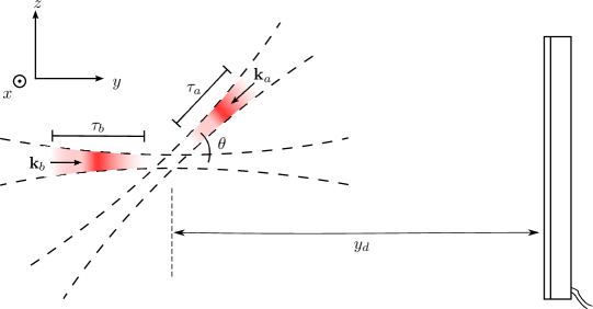
Fig. 1: The envisaged experimental set-up. $\tau_{a,b}$ refer to the pulse durations in the Gaussian beam envelopes $\mbox{e}^{-(t\pm y)^{2}/\tau_{a,b}^{2}}$, the $\mathbf{E}_{b}$ beam is displaced from the $y$-axis by co-ordinates $x_{0},z_{0}$, both beams have in general a carrier-envelope phase and the $\mathbf{E}_{a}$ beam lags behind $\mathbf{E}_{b}$ by $\Delta t$. The $\mathbf{E}_{b}$ field is incident on the detector.

We focus on the phenomenon of diffraction and specifically the detection of photons whose wave-vectors differ significantly, either in orientation or in magnitude from those of the background lasers. As such, we envisage an array of photosensitive detectors being placed some distance away from the collision, $y_{d}$, along the positive $y$-axis, much larger than the interaction volume (the subscript _d refers to quantities on the detector). $\mathbf{E}_{b}$ is then incident on this detector.

III Derivation of scattered field

When external electromagnetic fields polarising the vacuum have equivalent photon energies much less than the electron mass ($\hbar\omega\ll mc^{2}$), their evolution can be well-approximated by an effective description in which the vacuum fermion dynamics has been integrated out and only photon degrees of freedom remain. The Euler-Heisenberg Lagrangian Heisenberg and Euler [1936] is an effective Lagrangian which includes such fermion dynamics to one-loop order. When the field strength is much less than critical ($E\ll E_{cr}$), the Euler-Heisenberg Lagrangian can be well-approximated by its weak-field expansion, which, neglecting derivative terms, is:

$$\mathcal{L}=\frac{1}{8\pi}(E^{2}-B^{2})+\frac{1}{360\pi^{2}E_{cr}^{2}}\big{[}(E^{2}-B^{2})^{2}+7(\mathbf{E}\cdot\mathbf{B})^{2}\big{]}+O\Big{(}\frac{1}{E_{cr}^{4}}(E^{2}-B^{2})\Big{)}^{3}+O\Big{(}\frac{1}{E_{cr}^{4}}\mathbf{E}\cdot\mathbf{B}\Big{)}^{3}.$$ (4)

Fig. 2: The Euler-Heisenberg effective Lagrangian is an integration over the high-energy (fermion) degrees of freedom. The external field can be generated by multiple sources, indicated by photons in the diagram being with and without crosses.

The weak-field expansion Eq. (4) is depicted in Fig. 2 and can be understood as coupling the flux of electromagnetic fields from different sources with one another. Extremising Eq. (4) with respect to the photon gauge field returns the wave equation for $\mathbf{E}$ and $\mathbf{B}$ fields modified by the one-loop, weak-field, vacuum current, $\mathbf{J}_{\textrm{vac}}$:

$$\nabla^{2}\mathbf{E}-\partial_{t}^{2}\mathbf{E} = 4\pi\mathbf{J}_{\textrm{vac}}$$ (5)

$$\mathbf{J}_{\textrm{vac}} = \Big{[}\nabla\wedge\partial_{t}\mathbf{M}-\nabla(\nabla\cdot\mathbf{P})+\partial_{t}^{2}\mathbf{P}\Big{]},$$ (6)

where $\mathbf{P}=\frac{\partial\mathcal{L}}{\partial\mathbf{E}}-\frac{1}{4\pi}\mathbf{E}$, $\mathbf{M}=\frac{\partial\mathcal{L}}{\partial\mathbf{B}}+\frac{1}{4\pi}\mathbf{B}$ and

$$\mathbf{P} = \phantom{-}\frac{\alpha^{2}}{180\pi^{2}m^{4}}\big{[}2(E^{2}-B^{2})\mathbf{E}+7(\mathbf{E}\cdot\mathbf{B})\mathbf{B}\big{]}$$ (7)

$$\mathbf{M} = -\frac{\alpha^{2}}{180\pi^{2}m^{4}}\big{[}2(E^{2}-B^{2})\mathbf{B}-7(\mathbf{E}\cdot\mathbf{B})\mathbf{E}\big{]}.$$ (8)

Using the beam transversality, $\mathbf{k}_{c}\wedge\mathbf{E}_{c}=\mathbf{B}_{c}$, $\mathbf{P}$ and $\mathbf{M}$ can be written entirely in terms of the electric or magnetic field. One can then write the vacuum polarisation as a series $P_{i}=\chi^{(1)}_{ij}E_{j}+\chi^{(3)}_{ijkl}E_{j}E_{k}E_{l}+\ldots\chi^{(2n+1)}_{ij\cdots m}E_{j}\cdots E_{m}+\ldots$, where electric susceptibilities $\chi$ only occur at odd orders due to charge-conjugation symmetry (Furry’s theorem). Therefore, four-, six-, eight-, etc. wave mixing can in principle occur, although each extra order will be suppressed by a factor $\alpha(E/E_{cr})^{2}$.

An iterative approach can be used to solve Eq. (5), which, since $\mathbf{J}^{(0)}\propto[\alpha(E^{(0)}/E_{cr})^{2}]\mathbf{E}^{(0)}$ and $\alpha(E/E_{cr})^{2}\ll 1$, can be understood as perturbative:

$$\mathbf{E}^{(n+1)}(\mathbf{x}_{d},t_{d}) = \mathbf{E}^{(n)}(\mathbf{x}_{d},t_{d})+\int d^{3}x\frac{\mathbf{J}^{(n)}(\mathbf{E}^{(n)},\ldots,\mathbf{E}^{(0)})|_{t=t_{\textrm{ret}}}}{|\mathbf{x}-\mathbf{x}_{d}|},$$ (9)

where $\mathbf{E}^{(n)}$ is the $n$-th order perturbative solution of Eq. (5), $\mathbf{E}^{(0)}$ is the zero-field vacuum solution, obeyed by the Gaussian beams in vacuum, approximated by $\mathbf{E}_{a}$ and $\mathbf{E}_{b}$, $\mathbf{J}^{(n)}$ is the $n$-th iteration of the current occurring on the right hand side of the wave equation, $(\mathbf{x}_{d},t_{d})$ are the co-ordinates in the detector plane and $t_{\textrm{ret}}=t_{d}-|\mathbf{x}_{d}-\mathbf{x}|$ is the retarded time. By making the approximation that:

$$\mathbf{E}_{d}^{(n)}(\mathbf{x}_{d},t_{d})=\int d^{3}x\frac{\mathbf{J}^{(n)}(\mathbf{E}^{(n)},\ldots,\mathbf{E}^{(0)})|_{t=t_{\textrm{ret}}}}{|\mathbf{x}-\mathbf{x}_{d}|}\ll\mathbf{E}^{(0)},$$ (10)

for all $n$, the resultant electric field can be well approximated by $\mathbf{E}=\mathbf{E}^{(1)}=\mathbf{E}^{(0)}+\mathbf{E}_{d}$, $\mathbf{E}_{d}=\mathbf{E}_{d}^{(0)}$, i.e. the zero-field vacuum solution plus the lowest order “diffracted field.”

By substituting $\mathbf{E}^{(0)}=\mathbf{E}_{a}+\mathbf{E}_{b}$ in Eq. (6) and Eq. (9), and by enforcing the assumption that the dimensions of the interaction volume are much smaller than the typical detector co-ordinates, following similar steps to King et al. [2010b, a], Di Piazza et al. [2006], one arrives at:

$$\mathbf{E}_{d}(\mathbf{x}_{d},t_{d}) = -\frac{\alpha^{2}}{45\pi^{2}m^{4}r_{d}}\frac{1}{8i}\sum_{j=1}^{12}\Big{(}4+\omega_{j}^{2}\tau_{j}^{2}\Big{)}\frac{A_{j}}{\tau_{j}^{2}}E_{a,0}^{B_{j}}E_{b,0}^{\Gamma_{j}}\mathbf{v}_{l(j)}\mbox{e}^{i\psi_{j}}I_{t,j},$$ (11)

$$\widetilde{\mathbf{E}}_{d}(\mathbf{x}_{d},\omega) = -\frac{\alpha^{2}\omega^{2}}{45\pi^{3/2}m^{4}r_{d}}\frac{1}{8i}\sum_{j=1}^{12}A_{j}\tau_{j}E_{a,0}^{B_{j}}E_{b,0}^{\Gamma_{j}}\mathbf{v}_{l(j)}\mbox{e}^{i\psi_{j}}I_{\omega,j},$$ (12)

where $I_{t,j}$ and $I_{\omega,j}$ are integrals over the interaction volume, given in Eqs. (A.29) and (A.30), $r_{d}=|\mathbf{x}_{d}|$ is the detector distance, with $A_{j}\in\{-2,-1,1,2\}$, $B_{j},\Gamma_{j}\in\{1,2\}$ coefficients given in the appendix in Tab. 1, $\tau_{j}=[B_{j}/\tau_{a}^{2}+\Gamma_{j}/\tau_{b}^{2}]^{-1/2}$, $\omega_{j}=\beta_{j}\omega_{a}+\gamma_{j}\omega_{b}$, $\psi_{j}=\beta_{j}\psi_{a}+\gamma_{j}\psi_{b}$, $\beta_{j},\gamma_{j}\in\{-2,-1,0,1,2\}$ also given in Tab. 1 and $l(j)=1$ for $j<=6$, otherwise $l(j)=2$ and $\mathbf{v}_{1,2}$ are the diffracted field polarisation vectors given in Eqs. (A.27) and (A.28).

Splitting the plane-wave part of the input fields $\mathbf{E}_{a}$, $\mathbf{E}_{b}$ into positive and negative frequencies, the twelve terms in Eqs. (11) and (12) are produced, corresponding to the six possible orientations of the currents connected by the effective vertex in Fig. 2. As the interaction contains terms of the order $O[(\mathbf{E}_{a}+\mathbf{E}_{b})^{3}]$, and as the purely cubic terms $E_{a,b}^{3}$ necessarily disappear (both electromagnetic invariants are zero for the individual Gaussian beams, transverse in this approximation), for an incident current of frequency $\omega_{b}$, the resultant signal can have a frequency $\omega_{a},\omega_{b},\omega_{b}\pm 2\omega_{a},2\omega_{b}\pm\omega_{a}$, corresponding to the two beams’ elastic and inelastic components respectively. The diffracted field polarisation vectors $\mathbf{v}_{1,2}$ appear as geometrical factors and from their definition in Eqs. (A.27) and (A.28), one can see that on the detector ($y_{d}>0$), the $\omega_{a}$ and $\omega_{a}\pm 2\omega_{b}$ signal from pulse $a$ are strongly suppressed, as would be expected as the $\mathbf{E}_{a}$ pulse travels from the interaction region away from the detector. After a further analytical integration in $x$, the remaining two-dimensional integrals from Eqs. (A.29) and (A.30) were then evaluated numerically in C++, partly using the GSL library GNU Project - Free Software Foundation [2011].

One can interpret the classical field incident on the detector as being composed of a total number of photons $N_{t}$ by dividing its total energy by the photon energy so that $N_{t}=\int^{\infty}_{-\infty}d\omega dx_{d}dz_{d}\,\widetilde{I}_{t}(\omega,r_{d})/|\omega|$, where the total spectral density $\widetilde{I}_{t}(\omega,r_{d})=|\widetilde{\mathbf{E}}_{t}(\omega,r_{d})|^{2}/8\pi^{2}=|\widetilde{\mathbf{E}}_{b}(\omega,r_{d})+\widetilde{\mathbf{E}}_{d}(\omega,r_{d})|^{2}/8\pi^{2}$ ($\widetilde{\mathbf{E}}_{a}(\omega,r_{d})$ is taken to be zero in the current beam set-up) and where $y_{d}$ is taken large enough that the surface perpendicular to the Poynting vector can be well approximated as being flat. Although the spectral density extends to negative frequencies, it is consistent to interpret the differential number of photons as this divided by the absolute frequency because the total energy is the integration over all frequencies and all energy is carried by positive-frequency photons (see also Jackson [1975] on this point). We then calculate the number of “accessible” photons that fall on the detector plane, by integrating over the annulus that satisfies $dN_{t}(x_{d},z_{d})-100\,dN_{b}(x_{d},z_{d})>0$ for $dN_{i}=\int_{-\infty}^{\infty}d\omega\,\widetilde{I}_{i}(\omega,r_{d})/|\omega|$, $i\in\{a,b,d,t\}$.

IV Elastic photon-photon scattering

Current and next generation high intensity lasers will typically produce pulses with many optical cycles and so unless some resonance condition is fulfilled, one would expect the elastic cross-section, where incident and outgoing spectra have the same form, to be the largest. By “elastic,” we are therefore referring to terms in $\mathbf{E}_{d}$ with equal incoming and outgoing frequencies. As an analytical test of our expressions, we can reproduce the electric field derived for the three-beam, double-slit cases given in King et al. [2010b, a] when the separation of the slits is sent to zero - the two-beam limit (this limit was calculated for King et al. [2010b] in King [2010]), which we label $\mathbf{E}_{d}^{h}$, $\mathbf{E}_{d}^{p}$ referring to head-on and perpendicular collisions respectively. By taking $x_{0}=z_{0}=\Delta t=0$ and the limit $\tau_{a,b}\to\infty$ in Eq. (11), with $\theta=0$, we recover $\mathbf{E}^{h}_{d}$ as given in King [2010], and with $\theta=\pi/2$, we recover $\mathbf{E}^{p}_{d}$ as given in King et al. [2010a]. As a numerical test of our expressions, we can compare $I_{d}(t,r_{d})=|\mathbf{E}_{d}(t,r_{d})\cdot\mathbf{E}_{d}(t,r_{d})|^{2}/4\pi$ in the case $I_{d}(0,r_{d})$ with results using the single-slit version of $\mathbf{E}_{d}^{h}$. The equivalent parameters are $\lambda_{a}=0.8~{}\mu\textrm{m}$, $\lambda_{b}=0.527~{}\mu\textrm{m}$, $w_{a,0}=0.8~{}\mu\textrm{m}$, $w_{b,0}=290~{}\mu\textrm{m}$, $P_{a}=50~{}\textrm{PW}$, $P_{b}=20~{}\textrm{TW}$, as the field strengths in King [2010], King et al. [2010a] were calculated using a conservative form of the beam intensity with power per unit area for an area $\pi\textrm{w}^{2}_{c,0}$, rather than the $\pi\textrm{w}^{2}_{c,0}/2$ which is manifest from an integration of the intensity of a Gaussian beam over the transverse plane. In order to obtain the agreement between $\mathbf{E}_{d}$ and $\mathbf{E}_{d}^{h}$ shown in Fig. 3, $\tau_{a,b}$ had to be set to around $10^{4}~{}\textrm{fs}$, which is unexpectedly large compared to the pulse durations considered in those references ($\tau_{a}=30~{}\textrm{fs}$, $\tau_{b}=100~{}\textrm{fs}$). We will elaborate the non-trivial dependency of $I_{d}$ on pulse duration, which explains why most of the difference between $I_{d}$ and $I_{d}^{h}$ disappears already at $\tau=10^{3}~{}\textrm{fs}$. When the number of accessible photons was calculated for the pulsed system with $\theta=0.1$ and the same durations as suggested in King [2010], the number of photons $N_{d}$ also fell from the estimated value of around $36$ to around $0.4$.

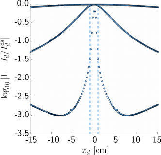
Fig. 3: Numerical comparison of $I_{d}$ with results in King [2010] (denoted $I_{d}^{\textrm{ds}}$). Plotted is $\log_{10}$ of the absolute relative difference in $I_{d}$, for, from top to bottom, $\tau_{a}=\tau_{b}=100~{}\textrm{fs}$, $1000~{}\textrm{fs}$ and $20000~{}\textrm{fs}$. Between the dotted lines, the background dominates ($I_{b}\gg I_{d}$).

To illuminate the two orders of magnitude difference in $N_{d}$ for these parameters, the integrand for $\mathbf{E}_{d}$ was reduced to the most significant terms for a head-on, elastic collision and evaluated independently in Mathematica. The simplified expression $\widehat{N}_{d}(\tau)$ was then

$$\widehat{N}_{d}(\tau) = \int^{\rho^{\textrm{max}}_{d}}_{\rho^{\textrm{min}}_{d}}\!\!d\rho_{d}\rho_{d}\int_{-\infty}^{\infty}\frac{d\omega}{2\pi}~{}\Big{|}\int_{-\infty}^{\infty}dy~{}\frac{\sqrt{\pi}\tau}{\sqrt{3}}\mathcal{V}(y,\omega,\omega_{b},\tau,\rho_{d}/r_{d})\Big{|}^{2}$$ (13)

$$\widehat{N}_{d}^{h}(\tau) = 2\int^{\rho^{\textrm{max}}_{d}}_{\rho^{\textrm{ min}}_{d}}\!\!d\rho_{d}\rho_{d}~{}\frac{\tau}{4}~{}\Big{|}\int_{-\infty}^{\infty}dy\lim_{\tau\to\infty}\lim_{\omega_{b}\to\omega}\mathcal{V}(y,\omega,\omega_{b},\tau,\rho_{d}/r_{d})\Big{|}^{2}$$ (14)

$$\mathcal{V}(y,\omega,\omega_{b},\tau,\rho_{d}/r_{d}) = \frac{\alpha I_{a,0}E_{b,0}w_{a,0}^{2}\omega^{3/2}}{360\pi y_{d}I_{cr}i}\Big{[}1+\frac{1}{2}\frac{w^{2}_{a,0}}{w^{2}_{b,0}}\frac{1+(y/y_{r,a})^{2}}{1+(y/y_{r,b})^{2}}\Big{]}^{-1}$$ (15)

$$\textrm{exp}\Big{[}\frac{-\omega^{2}\rho_{d}^{2}(1+(y/y_{r,a})^{2})}{4r_{d}^{2}\big{[}2+\frac{w^{2}_{a,0}}{w^{2}_{b,0}}\frac{1+(y/y_{r,a})^{2}}{1+(y/y_{r,b})^{2}}\big{]}}+\frac{4i(\omega-\omega_{b})y}{3}-\frac{8y^{2}}{3\tau^{2}}-\frac{(\omega-\omega_{b})^{2}\tau^{2}}{12}\Big{]},$$

where $s^{2}=(2/w_{a,0}^{2}+1/w_{b,0}^{2})^{-1}$, $\rho_{d}^{2}=(x_{d}^{2}+z_{d}^{2})/r_{d}^{2}$ and $\widehat{N}_{d}^{h}$ is equivalent to the expression leading from $\mathbf{E}_{d}^{h}$. The dependence on $\rho_{d}/r_{d}$ of these two expressions is shown in Fig. 4(a), where it can be seen that the monochromatic $\widehat{N}_{d}^{h}$ is much larger and more sharply peaked in the centre of the detector.

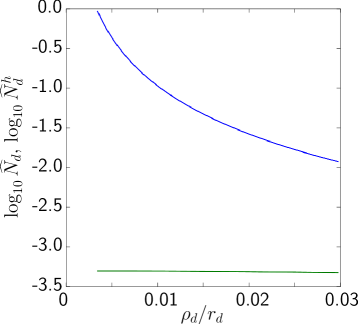
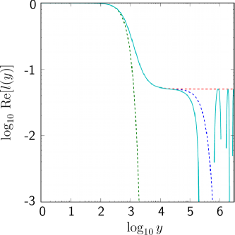
Fig. 4: Left-hand plot (a): $\log_{10}\widehat{N}_{d}^{h}$ (upper curve) and $\log_{10}\widehat{N}_{d}$ (lower curve) plotted against $\rho_{d}$. Right-hand plot (b): a log-log-plot of $\textrm{Re}\,[l(y)]$ (solid line) with the first, second and third dashed lines corresponding to $\lim_{w_{b,0}\to\infty}l(y)$, $|l(y)|$ and $\lim_{y_{r,b}\to\infty}l(y)$.

After integrating between the relevant annulus of $\rho_{d}^{(\textrm{min})}/r_{d}=0.0032$ and $\rho_{d}^{(\textrm{max})}/r_{d}=0.03$, this independent test then gives $\widehat{N}_{d}(\tau)=0.33$ and $\widehat{N}_{d}^{h}=37.0$. The corresponding values for a circular detector of radius $15~{}\textrm{cm}$ from the full expression are $\widehat{N}_{d}(\tau)=0.33$ and $\widehat{N}_{d}^{h}=38.0$, supporting the two-orders of magnitude difference and the claim that Eqs. (13-15) incorporate the main physics. By plotting the exponential dependency on $\rho_{d}/r_{d}$, which is integrated over to acquire the expected number of photons in the monochromatic case, $\widehat{N}_{d}^{h}$:

$$l(y)=\textrm{exp}\Big{[}-\frac{\omega^{2}\rho_{d}^{2}(1+(y/y_{r,a})^{2})}{4\big{[}2+\big{(}\frac{w_{a,0}}{w_{b,0}}\big{)}^{2}\frac{1+(y/y_{r,a})^{2}}{1+(y/y_{r,b})^{2}}\big{]}}\Big{]},$$ (16)

we observe the interesting behaviour shown in Fig. 4(b). We first note that the decay is not purely exponential, but has two important length scales: $w_{b,0}$ and $y_{r,b}$, which, in the limit of being infinitely large, correspond to the first and third dashed curves in Fig. 4(b). The inclusion of these extra longitudinal length scales in King [2010], which cannot contribute to photon scattering when the finite pulse length is taken into consideration, then explains the discrepancy in the values of $\widehat{N}_{d}(\tau)$ and $\widehat{N}_{d}^{h}$. Only the region of the pulses within a distance $\tau$ around their maxima in the longitudinal direction can efficiently contribute to the scattering process, with the rest of the pulse being damped by its Gaussian shape. The finite length of laser pulses probing vacuum photon-photon scattering can then only be neglected, when the duration $\tau$ is the largest longitudinal length scale. In the limit $\tau\gg y_{r,b}$ in the full expression for $\mathbf{E}_{d}$ in Eqs. (11) and (12), the scaling $N_{d}(\tau)\propto\tau$ of King [2010] is recovered, supporting this statement (this will also be apparent from Fig. 5). Furthermore, the results of King [2010] are expected to remain valid in the case $\pi w_{b,0}^{2}/\lambda_{b}\tau_{a,b}<1$, so for more focused and longer wavelength probe beams as well as for longer pulses. Indeed for the parameters quoted, that the effect would be two orders of magnitude weaker is in no way prohibitive to conducting such experiments. For example in King et al. [2010b], King [2010], the intensity of the probe beam was taken to be only around $I_{p}\approx 10^{16}~{}\textrm{Wcm}^{-2}$, but as $N_{d}\propto I_{p}$, the shortfall could be made up by focusing the probe beam more (if $w_{b,0}$ is set to $60~{}\mu\textrm{m}$, $N_{d}$ increases approximately by a factor $7$ in the single-slit and $4.5$ in the double-slit case) or increasing the power of the probe (from $10~{}\textrm{TW}$), to which $N_{d}$ is proportional.

The current treatment also allows for the two lasers to be equally strong and we consider the more experimentally-accessible situation of having a single laser, split into two colliding pulses, both focused to ultra-high intensities. Since $N_{d}$ scales with $E_{a,0}^{2B_{j}}E_{b,0}^{2\Gamma_{j}}$ if we keep the power of the laser constant ($E_{c,0}=2\sqrt{2P_{c,0}}/w_{c,0}$), for each term, the optimal division of the total power between the beams is:

$$\frac{P_{a,0}}{P_{b,0}}=\frac{B_{j}}{\Gamma_{j}};\qquad P_{a,0}=\frac{B_{j}}{B_{j}+\Gamma_{j}}P_{t,0}.$$ (17)

For base parameters similar to that of the Vulcan laser Vulcan [2010] $\lambda_{a}=\lambda_{b}=0.91~{}\mu\textrm{m}$, $\tau_{a}=\tau_{b}=30~{}\textrm{fs}$, $P_{a}=5~{}\textrm{PW}$, $P_{b}=5~{}\textrm{PW}$, with $w_{a,0}=0.91~{}\mu\textrm{m}$, $w_{b,0}=100~{}\mu\textrm{m}$, $\hat{\boldsymbol{\varepsilon}}_{a}=\hat{\boldsymbol{\varepsilon}}_{b}=\hat{\mathbf{x}}$ a summary of the dependency of $N_{d}$ on several variables is given in Fig. 5. We will comment on the plots sequentially, in which solid lines represent what one could intuitively expect, as explained in the following. Starting from the right-hand side of the first plot and moving in the direction of falling $w_{b,0}$, we see $N_{d}(w_{b,0})$ increases approximately as $\propto w_{b,0}^{-2}$, indicated by the solid line. Since $N_{d}$ for such a set-up is proportional to $E_{b,0}^{2}$, and since this is inversely proportional to the area of focusing, the dependency on $\propto w_{b,0}^{-2}$ is as expected. Deviation occurs when a maximum is reached (see e.g. King et al. [2010a] for details), beyond which $N_{d}(w_{b,0})$ falls rapidly as the background from $\mathbf{E}_{b}$ gradually covers the entire detector, leaving no signal. The dependency on beam-separation $N_{d}(x_{0})$ is also intuitive and seen to have excellent agreement with a Gaussian, normalised in height, with a width of $w_{b,0}/2$ ($\exp(-2x_{0}^{2}/w_{b,0}^{2})$). Simply by integrating the transverse Gaussian distributions of the two beams, and then squaring ($N_{d}\propto|\mathbf{E}_{d}|^{2}$), one arrives at this dependency. The third plot of $N_{d}(\lambda)$ ($\lambda=\lambda_{a}=\lambda_{b}$) is a log-log plot where the dependency begins for small $\lambda$ as $N_{d}\approx\lambda^{-3}$ but then for larger values tends to $N_{d}\approx\lambda^{-3.5}$. This is shown by all the points lying between these two solid lines. Since the power of each beam is inversely proportional to wavelength, and since the $N_{d}\propto P_{a,0}^{2}P_{b,0}$, one would expect at least a dependency of $N_{d}(\lambda)\sim\lambda^{-3}$. In contrast, the dependency of $N_{d}(\tau)$ can be straightforwardly derived. For $\tau_{a}=\tau_{b}=\tau$, one notes that when $\tau\ll w_{b,0},y_{r,b}$, the interaction volume in beam propagation direction is governed by the Gaussian pulse shape. Further noting that $N_{d}$ essentially involves a double integration on longitudinal beam co-ordinate (through taking the mod-squared), as well as an integral over $t$, the dependency $N_{d}(\tau)\propto\tau^{3}$ appears, which shows excellent agreement for small $\tau$ with the full numerical integration, displayed by the on the log-log plot of $N_{d}(\tau)$ in the fourth figure. The larger $\tau$ is for $\tau>w_{b,0}$, the more the decay along the beam propagation axis is described by focusing rather than pulse terms. For large enough $\tau$, $I_{d}$ depends only on focusing terms and since the yield $N_{d}$ is acquired from an integration over time, we have $N_{d}(\tau)\propto\tau$ and this transition can be seen by the second, linear, fit line for large $\tau$ in the figure. An estimation of the dependency of $N_{d}(\theta)\propto(1+\cos\theta)^{2}$ on beam intersection angle comes from the geometrical factor in $\mathbf{v}_{1}\propto(1+\cos\theta)$, which must be squared and gives the approximate agreement shown in the fifth plot. For small angles $N_{d}(\theta)\propto 1-\theta^{2}/2$, making the dependency relatively weak for near head-on collisions ($N_{d}$ remains at $90\,\%$ of its value up to $\theta\approx\pi/7$). The final plot of $N_{d}(\Delta t)$ closely resembles a Gaussian with width $9\tau$ and so for this set-up, $N_{d}$ is relatively insensitive to lag.

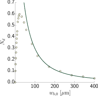
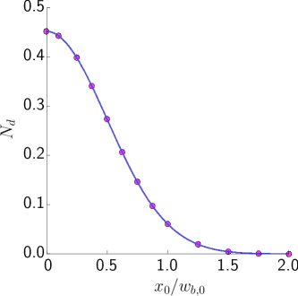
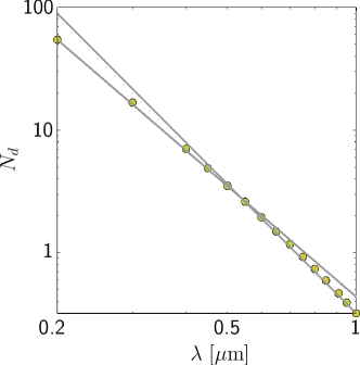
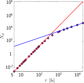
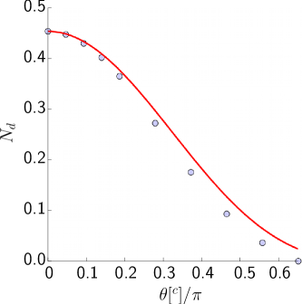
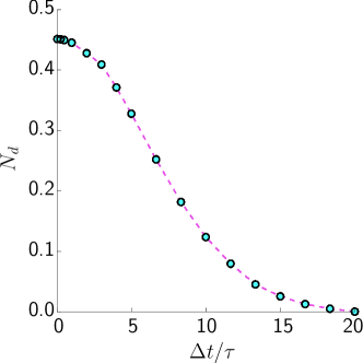
Fig. 5: Dependency of the number of measurable elastically diffracted photons $N_{d}$ on various parameters, where parameters held constant take the values $\lambda_{a}=\lambda_{b}=0.91~{}\mu\textrm{m}$, $w_{a,0}=0.91~{}\mu\textrm{m}$, $w_{b,0}=100~{}\mu\textrm{m}$, $\tau_{a}=\tau_{b}=30~{}\textrm{fs}$, $P_{a}=5~{}\textrm{PW}$, $P_{b}=5~{}\textrm{PW}$, $\hat{\boldsymbol{\varepsilon}}_{a}=\hat{\boldsymbol{\varepsilon}}_{b}=\hat{\mathbf{x}}$.

One strategy to increase the number of diffracted photons would be to use higher-harmonics of the probe laser. If the same parameters as in Fig. 2 are used, for a collision angle of $\theta=0.1$, assuming a $40\%$ reduction in energy due to generating the second harmonic, $N_{d}\approx 4$. If this process could be repeated to generate the fourth-harmonic, with a $16\%$ reduction, $N_{d}\approx 13$. As previously argued in King et al. [2010b], such numbers of scattered photons should allow detection in experiment. A discussion of sources of background noise and why they can be effectively neglected is given in King et al. [2010b], King [2010].

V Inelastic photon-photon scattering (four-wave mixing)

When considering the possible frequencies of the resultant current, conservation of energy and linear momentum leads one to the equations:

$$\omega = \textrm{sgn}(\beta_{j})[\omega_{a,1}+\delta_{|\beta_{j}|2}\omega_{a,2}]+\textrm{sgn}(\gamma_{j})[\omega_{b,1}+\delta_{|\gamma_{j}|2}\omega_{b,2}]$$ (18)

$$\omega\,\frac{y_{d}}{r_{d}} = \textrm{sgn}(\beta_{j})[\omega_{a,1}\cos\theta_{a,1}+\delta_{|\beta_{j}|2}\omega_{a,2}\cos\theta_{a,2}]$$ (19)

$$+~{}\textrm{sgn}(\gamma_{j})[\omega_{b,1}\cos\theta_{b,1}+\delta_{|\gamma_{j}|2}\omega_{b,2}\cos\theta_{b,2}]$$

$$\omega\,\frac{\rho_{d}}{r_{d}} = \textrm{sgn}(\beta_{j})[\omega_{a,1}\sin\theta_{a,1}+\delta_{|\beta_{j}|2}\omega_{a,2}\sin\theta_{a,2}]$$ (20)

$$+~{}\textrm{sgn}(\gamma_{j})[\omega_{b,1}\sin\theta_{b,1}+\delta_{|\gamma_{j}|2}\omega_{b,2}\sin\theta_{b,2}],$$

where $\omega$ is the frequency of the resultant current, $\textrm{sgn}(x)$ returns the sign of $x$ with $\textrm{sgn}(0)=0$, and $\theta_{\{a,b\},\{1,2\}}$ are the angles the currents make with $\hat{\mathbf{y}}$. Therefore, detection co-ordinate, focusing and harmonic order are already linked at this stage. It turns out to be difficult to satisfy these conditions simultaneously with just two laser beams and a fixed observation angle. For example, if we take $\beta_{j}=2$, $\gamma_{j}=1$, with $\omega_{a,1}=\omega_{a,2}=\omega_{a}$, $\omega_{b,1}=\omega_{b,2}=\omega_{b}$ for simplicity and a more-or-less head-on collision of the lasers, so $\theta_{a,\{1,2\}}$ is approximately equal to $\pi-\theta_{b,\{1,2\}}$ and $\theta_{b,\{1,2\}}$ is small, then, to first order, from Eqs. (18) and (19) we have $\omega=2\omega_{a}+\omega_{b}$ and $\omega\,y_{d}/r_{d}\approx-2\omega_{a}+\omega_{b}$. Since $y_{d}/r_{d}\approx 1$ on the detector, the contribution from this term can therefore only be satisfied by a small range of frequencies around $\omega_{a}=0$, which are not typically populated in the spectrum of $\mathbf{E}_{a}$. The energy-momentum conditions Eqs. (18-20) can be most easily seen occurring in the exponent of the integral $I_{\omega}$ Eq. (A.30), where they appear as frequencies of plane waves to be integrated over in $y$, $z$, becoming Gaussian-like after integration. The larger the deviation from these conditions, the higher the frequency of oscillation to be integrated over, the more exponentially small the resulting amplitude, typical for evanescent waves.

We investigated the ansatz that for short enough pulses, the bandwidth of the two lasers becomes wide enough that Eqs. (18-20) can be fulfilled simultaneously for a measurable amount of photons. Essentially, for this four-wave interaction, three different photon energies can be supplied by two lasers. To make this statement explicit, instead of using a temporal envelope, we can consider building the pulses in the frequency domain:

$$\mathbf{E}^{\prime}_{c}(\mathbf{x},t)=\int^{\infty}_{-\infty}d\omega_{c}\,\mathbf{E}^{\textrm{mono}}_{c}(\mathbf{x},t,\omega_{c})g(\omega_{c},\omega_{c,0}),$$ (21)

where $\mathbf{E}^{\textrm{mono}}_{c}(\mathbf{x},t,\omega_{c})$ is the electric field of a monochromatic Gaussian beam, frequency $\omega_{c}$ and $g(\omega_{c},\omega_{c,0})$ is the spectral density of the pulse $\mathbf{E}^{\prime}_{c}(\mathbf{x},t)$, with peak frequency $\omega_{c,0}$. Then due to our interaction being cubic in the fields ($\mathbf{E}_{a}^{B_{j}}$, $\mathbf{E}_{b}^{\Gamma_{j}}$), the integration over this current in the frequency domain, Eq. (A.30), would include three extra integrations over frequency $\int d\omega_{a}d\omega_{b}d\omega_{c}\,g(\omega_{a},\omega_{a,0})\,g(\omega_{b},\omega_{b,0})\,g(\omega_{c},\delta_{B_{j}2}\omega_{a,0}+\delta_{\Gamma_{j}2}\omega_{b,0})\,\delta(\omega-\omega_{j})$, where the final delta function appears explicitly from an integration over $t$. Here it is apparent that due to the finite bandwidth, in general, three different energies enter the effective vertex in Fig. 2 from the two lasers. If the spectrum is taken to be Gaussian $g(\omega_{c},\omega_{c,0})=\exp[-(\omega_{c}-\omega_{c,0})^{2}\tau_{c}^{2}/4]\tau_{c}/2\sqrt{\pi}$ we have, setting $\theta=0$ without loss of generality:

$$\mathbf{E}^{\prime}_{c}(\mathbf{x},t) = \hat{\boldsymbol{\varepsilon}}_{c}\int_{-\infty}^{\infty}\!\!d\omega_{c}\frac{1}{2i}\frac{E_{c,0}\,\mbox{e}^{-\frac{x^{2}+z^{2}}{w_{c}^{2}(y)}-(\omega_{c}-\omega_{c,0})^{2}\frac{\tau_{c}^{2}}{4}}}{\sqrt{1+(y/y_{r,c})^{2}}}\mbox{e}^{i(\omega_{c}(y-t)+\tan^{-1}\frac{2y}{\omega_{c}w_{c,0}^{2}}-\frac{2\omega_{c}y(x^{2}+z^{2})}{4y^{2}+\omega_{c}^{2}w_{c,0}^{4}y^{2}})}+\textrm{c. c.}.$$

$$= \frac{E_{c,0}\,\mbox{e}^{-\frac{x^{2}+z^{2}}{w_{c}^{2}(y)}-(\frac{y-t}{\tau_{c}})^{2}}}{\sqrt{1+(y/y_{r,c})^{2}}}\sin\Big{[}\omega_{c,0}(y-t)+\tan^{-1}\frac{y}{y_{r}}-\frac{\omega_{c,0}y}{2}\frac{x^{2}+z^{2}}{y^{2}+y_{r}^{2}}\Big{]}+\textrm{h. o. t.},$$

where the remaining terms are of the same order as those neglected in the Gaussian beam solution. Therefore the use of a Gaussian temporal envelope in $\mathbf{E}_{a}$ and $\mathbf{E}_{b}$ (Eqs. (1) and (2)), is equivalent to integrating over three different photon frequencies from the external fields in the interaction.

When $x_{0}=z_{0}=\Delta t=\theta=0$, $y_{r}=y_{r,a}=y_{r,b}$ and $\rho_{d}^{2}/r_{d}^{2}=(x_{d}^{2}+z_{d}^{2})/r_{d}^{2}$ is small, $dN_{d}(x_{d},z_{d})$ can be approximated analytically. We can write $dN_{d}(x_{d},z_{d})=\sum_{p,q=1}^{12}dN^{pq}_{d}(x_{d},z_{d})$ and demonstrate this analysis by concentrating on a single term $N_{d}^{qq}$ for convenience (the full expression is given in Eq. (A.35)). One can show:

$$dN^{qq}_{d}(x_{d},z_{d}) \approx \frac{2}{\pi^{2}}\Bigg{[}\frac{\alpha A_{q}}{90}\frac{E_{a,0}^{B_{q}}E_{b,0}^{\Gamma_{q}}}{E_{cr}^{2}}\frac{|\mathbf{v}_{l(q)}|}{16}\frac{w_{a,0}^{2}}{sr_{d}}\frac{\tau_{q}^{2}}{\sqrt{1-\tau_{qq}^{4}}}\Bigg{]}^{2}\mbox{e}^{-\frac{\omega_{q}^{2}\tau^{2}}{2}[1+\frac{(\tilde{\omega}_{qq}-\tau_{qq}^{2})^{2}}{1-\tau_{qq}^{4}}]}$$ (22)

$$\int^{\infty}_{-\infty}d\omega|\omega|^{3}\mbox{e}^{-[\frac{\rho_{d}^{2}\textrm{w}^{2}_{a,0}}{2sr_{d}^{2}}+\frac{\tau_{q}^{2}}{2}+\frac{\tau_{q}^{2}(\tau_{qq}^{2}+y_{d}/r_{d})^{2}}{2(1-\tau_{qq}^{4})}]\omega^{2}+\tau_{q}^{2}\omega_{q}[1-\frac{(y_{d}/r_{d}+\tau_{qq}^{2})(\tilde{\omega}_{qq}-\tau_{qq}^{2})}{1-\tau_{qq}^{4}}]\omega},$$

where $s=1/(B_{j}+\Gamma_{j}(w_{a,0}/w_{b,0})^{2})$, $\tau_{qq}=\tau_{q}/\tilde{\tau}_{q}$, $\tilde{\tau}_{q}^{2}=(B_{q}/\tau_{a}^{2}-\Gamma_{q}/\tau_{b}^{2})^{-1}$ and $\tilde{\omega}_{qq}=\tilde{\omega}_{q}/\omega_{q}$, $\tilde{\omega}_{q}=\beta_{q}\omega_{a}-\gamma_{q}\omega_{b}$, under the condition $T^{2}/y_{r}^{2}\ll 1$, for $T^{2}=\tau_{q}^{2}[1-\tau_{qq}^{s4}]^{-1}$ and where a condition on $\omega$: $|[\omega(\tau_{qq}-y_{d}/r_{d})+\tilde{\omega}_{q}-\omega_{q}\tau_{qq}^{2}]T^{2}/y_{r}|\ll 1$ has been approximated by taking the upper limit of the integration as $\infty$. To simplify the discussion, let $\tau_{a}=\tau_{b}=\tau$. Then we can see from Eq. (22) that the spectral density for inelastically scattered photons has a different shape to the background, namely with a minimum at $\omega=0$ and two maxima, whose positions for the case $x_{d}=z_{d}=0$ are $\omega^{\pm}=(\gamma_{q}\omega_{b}/2)(1\pm[1+12/(\gamma_{q}\omega_{b}\tau)^{2}]^{1/2})$. Using a spectral filter, and short enough pulses, this could in principle be used to separate the different inelastic scattering signals from each other and the elastically scattered and background photons on the detector. Setting $\rho_{d}=0$ for brevity, the final integral can be approximated by:

$$dN^{qq}_{d}(x_{d},z_{d}) = \sqrt{\frac{2}{\pi^{3}}}\Bigg{[}\frac{\alpha A_{q}}{180}\frac{E_{a,0}^{B_{q}}E_{b,0}^{\Gamma_{q}}}{E_{cr}^{2}}\frac{|\mathbf{v}_{l(q)}|}{16}\frac{w_{a,0}^{2}}{sr_{d}}\Bigg{]}^{2}\big{(}\gamma_{q}\omega_{b}\tau\big{)}[3+(\gamma_{q}\omega_{b}\tau)^{2}]$$ (23)

$$\qquad\qquad\qquad\qquad\qquad\qquad\qquad\textrm{Erf}\Bigg{[}\frac{\gamma_{q}\omega_{b}\tau}{\sqrt{2}}\Bigg{]}\mbox{e}^{-\frac{1}{4}(\beta_{q}\omega_{a}\tau)^{2}-\frac{1}{18}(\gamma_{q}\omega_{b}\tau)^{2}}$$

It should be noted that $\mathbf{v}_{l(j)}$ is identically zero for $j>6$ at $r_{d}=y_{d}$, and so the frequencies $\omega_{a}$, $2\omega_{b}\pm\omega_{a}$ are suppressed, as already argued. The numerical integration of the full highly-oscillating integrands was performed using the Filon method, which is an approximation to the integral $\int dtf(t)\cos(\omega t)$ for asymptotically-large $\omega$ (see e.g. Davis and Rabinowitz [1967]), used with the GNU arbitrary-precision C++ library Enge et al. [2011]. Agreement between numerics and analytics for $w_{a,0}=w_{b,0}=10~{}\mu\textrm{m}$, $y_{d}=1~{}\textrm{m}$, $\beta_{q}=2$, $\gamma_{q}=1$ is then shown in Fig. 6, in part corroborating our numerical approach.

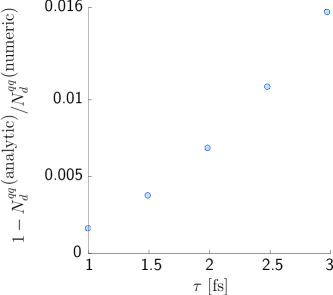
Fig. 6: Agreement of the analytical approximation Eq. (23) with the corresponding numerical solution.

The pulse duration of each laser plays an important role in four-wave mixing. By choosing a temporal profile for the beam that is Gaussian, we already have implicitly the lower bound $\tau\gg 1/\omega$. As pulse duration and longitudinal co-ordinate are linked, a natural upper bound is also formed for our calculation in the assumption that the diffracted field is smaller than the vacuum-polarising fields Eq. (10). Assuming scattered photons arriving at a point on the detector are generated in the centre of the beams’ intersection, the integration is exclusively over regions in which the polarising beams are more intense than the diffracted field when $\tau\ll 2w_{b,0}y_{d}/\rho_{d}$, giving $1/\omega\ll\tau\ll 2w_{b,0}y_{d}/\rho_{d}$. The lower bound limits our ability to assess the importance of the inelastic process. We require a large bandwidth $\Delta\omega/\omega$ for the inelastically-generated photons to be on-shell, but from the bandwidth theorem, $\Delta\omega/\omega\sim 1/\omega\tau\ll 1$ by our limitation on $\tau$. As a consequence, with a two-beam set-up, spectrally separating off the inelastic signal would be experimentally challenging, as this signal is generated when the bandwidth of the elastic background overlaps these “inelastic” frequencies. More promising seems to be to observe the change in $N_{d}$ due to inelastic scattering becoming significant as $\tau$ is reduced. In Fig. 7, we plot this ratio $(N_{t}-N_{e})/N_{e}$ against $\tau_{a}$, where $N_{e}$ is the number of photons scattered due to when only the elastic terms are included in Eq. (12). The results suggest that for short enough pulse durations, the inelastic process can influence the total number of measured photons substantially. In Fig. 7 the proportion reaches over 20%, for a minimum pulse duration of $\tau=1~{}\textrm{fs}$, equivalent to $\omega_{a}\tau_{a}\approx 2$. This could already have been anticipated from $\mathbf{E}_{d}(\mathbf{x}_{d},t_{d})$ in Eq. (11), including, as it does, a pre-factor $4+(\omega_{j}\tau_{j})^{2}$. In addition, although the pulse durations are short, assuming again $40\%$ attenuation each time a second-harmonic is generated from the probe, the total number of diffracted photons ranges from $1$ to $4$ (at $\tau_{a}=1$, $2$ respectively). Although the analysis is limited by how small $\tau_{a}$ can be consistently made, these results lend support to the ansatz that two laser beams with a large bandwith, especially in the laser being probed, can be used to measure the effect of the inelastic process.

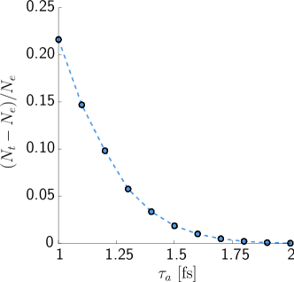
Fig. 7: The increasing importance of the inelastic process with increasing bandwidth. Plotted is the proportion of the total number of diffracted photons that are due to inelastic scattering, against $\tau_{a}$, for $P_{b}=10/3~{}\textrm{PW}$, $P_{a}+P_{b}=10~{}\textrm{PW}$, $\lambda_{a}=0.91~{}\mu\textrm{m}$, $\lambda_{b}=0.2275~{}\mu\textrm{m}$, $\tau_{b}=2~{}\textrm{fs}$, $w_{a,0}=0.91~{}\mu\textrm{m}$, $w_{b,0}=50~{}\mu\textrm{m}$, $\boldsymbol{\varepsilon}_{a}=(1,0,0)$, $\boldsymbol{\varepsilon}_{b}=(0,0,1)$, $\psi_{a}=\psi_{b}=0$.

In order to further support this ansatz and without being limited by a minimum value of the pulse duration, we can consider the simplified case of the collision of two plane waves modulated by a sech envelope.

$$\mathbf{E}_{a}(y+t) = \hat{\boldsymbol{\varepsilon}}_{a}\,E_{a,0}\cos(\omega_{a}(y+t))\,\textrm{sech}\Big{[}\frac{y+t}{\tau_{a}}\Big{]}$$ (24)

$$\mathbf{E}_{b}(y-t) = \hat{\boldsymbol{\varepsilon}}_{b}\,E_{b,0}\cos(\omega_{b}(y-t))\,\textrm{sech}\Big{[}\frac{y-t}{\tau_{b}}\Big{]}.$$ (25)

These fields satisfy Maxwell’s vacuum equations exactly, therefore removing the limitations on conceivable pulse lengths brought about by using a perturbative solution. The analysis proceeds just as for the Gaussian case but with the difference that now the fields are not bound in the transverse plane. Therefore, in order to avoid a divergence, we only consider the resulting $\mathbf{P}$ and $\mathbf{M}$ to be non-zero up to a finite transverse radius $\rho_{0}$. It can be shown that this curtailing of the interaction region then allows us to integrate over the current Eq. (9) as usual. The diffracted field $\widetilde{\mathbf{E}}^{\textrm{sech}}_{d}(\mathbf{x}_{d},\omega)$ then becomes:

$$\widetilde{\mathbf{E}}^{\textrm{sech}}_{d}(\mathbf{x}_{d},\omega) = -\frac{\omega^{2}\alpha^{2}}{45\pi^{2}m^{4}r_{d}}\frac{1}{8i}\sum_{j=1}^{2}E_{a,0}^{3-j}E_{b,0}^{j}\mathbf{v}_{j}I^{\textrm{sech}}_{\omega,j},$$ (26)

where $\mathbf{v}_{j}$ are geometrical factors as in the Gaussian case Eqs. (A.27) and (A.28), $I^{\textrm{sech}}_{\omega,j}$ are integrals given in Eq. (A.36), the sum over $j$ corresponds to the two terms $E_{a,0}^{2}E_{b,0}$ and $E_{a,0}E_{b,0}^{2}$ respectively and $z_{d}=0$ has been set for simplicity. Unlike for Gaussian beams, the elastic scattering terms cannot be isolated so easily. In order to exemplify the effect of the inelastic process however, one can observe how the behaviour of $N^{(\textrm{sech})}_{d}$ changes as $\omega_{a}\tau_{a}$ is reduced to below unity. Deviation from “elastic” behaviour, indicates the importance of inelastic scattering.

The first plot in Fig. 8 depicts the dependence of $N^{\textrm{(sech)}}_{d}$ on $\tau_{a}$ and we notice that for $\omega_{a}\tau_{a}\lesssim 2$ ($\tau_{a}\lesssim 0.8~{}\textrm{fs}$), there is indeed a deviation in the behaviour of $N^{\textrm{(sech)}}_{d}$. We can take data from a more uniform region $\tau_{a}>1~{}\textrm{fs}$ and acquire a best-fit polynomial with the boundary condition $N^{\textrm{(sech)}}_{d}(\tau_{a}=0)=0$. It turns out that a cubic polynomial fits the calculated points well (similar to the Gaussian beam case where $N_{d}(\tau)\propto\tau^{3}$). When the fit parameters were calculated for $1~{}\textrm{fs}<\tau_{a}<2~{}\textrm{fs}$, the goodness-of-fit was tested with a Pearson’s chi-squared test over $1~{}\textrm{fs}<\tau_{a}<3~{}\textrm{fs}$ and found to support the hypothesis of agreement with a probability of over $0.995$. When the relative difference of this “elastic” curve from the total was calculated, the second plot in Fig. 8 was generated. This clearly demonstrates the new behaviour occurring for short pulse durations or equivalently large bandwidths and so further supports our initial ansatz that just one beam split into two counter-propagating sub-cycle pulses is sufficient for accessing the process of vacuum inelastic photon-photon scattering. A suggestion for further work would be to investigate the role of the carrier-envelope phase as well as a chirped frequency.

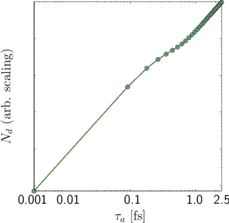
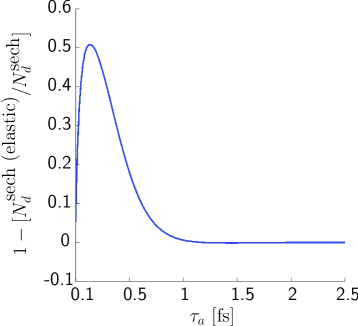
Fig. 8: On the left, for $N_{d}^{\textrm{sech}}(\tau_{a})$, with $\tau_{b}=1.4~{}\textrm{fs}$, at $x_{d}=0.1\,r_{d}$, $z_{d}=0$, $y_{d}=1~{}\textrm{m}$ and $\lambda_{a}=\lambda_{b}=0.8~{}\mu\textrm{m}$, the dominant term $E_{a}^{2}E_{b}$ has been plotted and the coefficient of the integral ignored. On the right is plotted the relative difference between the “elastic” and full behaviour of $N_{d}^{\textrm{sech}}(\tau_{a})$.

VI Summary

In calculating numbers of photons scattered in the collision of two laser beams, we had three aims: i) to consider a more realistic set-up of the colliding beams (including a temporal pulse shape, collision angle, lag and lateral separation), which would produce more accurate qualitative and quantitative predictions for experiment, ii) to investigate the possibility of using a single laser, split into two beams to measure elastic photon-photon scattering and iii) to evaluate the ansatz that just two lasers, with sufficiently short pulse durations, can be used to measure the process of inelastic photon-photon scattering. The first of these aims has been met in Fig. 5 where the dependency on various collision parameters was calculated and found consistent with physical reasoning. This led to the second aim, where the inclusion of a pulse form and collision angle led to two orders of magnitude difference over previous elastic photon scattering estimates King [2010] (the single-slit limit of King et al. [2010b]). In this more complete description, it was shown that when a $10~{}\textrm{PW}$, $\lambda=0.91~{}\textrm{nm}$ beam is separated into two $30~{}\textrm{fs}$ Gaussian pulses, incident at an angle $0.1$, one could expect approximately $0.7$, $4$ or $13$ photons, corresponding to the fundamental, second and fourth harmonic of the probe respectively (with an assumed loss of $40\,\%$ per frequency doubling), to be diffracted into detectable regions. As argued in King et al. [2010b], this could be sufficient for measuring elastic photon-photon scattering, here shown using a single $10~{}\textrm{PW}$ source. The final aim was partially met, first by considering Gaussian pulses, where it was shown that for $\omega\tau_{a}\lesssim 4$ for the more intense beam $a$, the inelastic scattering process increased and became as large as around $20$% that of the elastic count for $\omega\tau_{a}\approx 2$. However, for these results to be consistent, $\omega\tau_{a}\gg 1$, so the head-on collision of two sech pulses was analysed, for which no such bound applies, where it was shown that again, in this different field background, for $\omega\tau_{a}\approx 2$, inelastic scattering became important – as large as around $50$% that of the elastic one, lending supporting to our original ansatz.

VII Acknowledgements

B. K. would like to thank A. Di Piazza for his critical comments and careful reading of the manuscript.

Appendix A Integration formulae

A.1 Gaussian diffracted field formulae

Sum coefficients:

$j$	$\phantom{-}1$	$2$	$3$	$4$	$5$	$6$	$\phantom{-}7$	$8$	$\phantom{-}9$	$10$	$11$	$12$
$A_{j}$	$1$	$1$	$-2$	$-1$	$-1$	$2$	$1$	$1$	$-2$	$-1$	$-1$	$2$
$\beta_{j}$	$2$	$-2$	$0$	$2$	$-2$	$0$	$1$	$1$	$1$	$-1$	$-1$	$-1$
$\gamma_{j}$	$1$	$1$	$1$	$-1$	$-1$	$-1$	$2$	$-2$	$0$	$2$	$-2$	$0$

Table 1: Sum coefficients that occur in the expressions for $\mathbf{E}_{d}$ and $\widetilde{\mathbf{E}}_{d}$, Eqs. (11) and (12)

Diffracted field polarisation vectors:

$$\mathbf{v}_{1} = 4\Big{(}\hat{\boldsymbol{\varepsilon}}_{a}^{\prime}\cdot\hat{\boldsymbol{\varepsilon}}_{b}(1+\cos\theta)-\hat{\mathbf{y}}^{\prime}\cdot\hat{\boldsymbol{\varepsilon}}_{b}~{}\hat{\mathbf{y}}\cdot\hat{\boldsymbol{\varepsilon}}_{a}^{\prime}\Big{)}\Big{[}\hat{\boldsymbol{\varepsilon}}_{a}^{\prime}\Big{(}1-(\stackrel{{\scriptstyle\leftarrow}}{{\cdot}}\hat{\mathbf{r}}~{}\hat{\mathbf{r}})\Big{)}+(\hat{\mathbf{y}}^{\prime}\wedge\hat{\boldsymbol{\varepsilon}}_{a}^{\prime})\wedge\hat{\mathbf{r}}\Big{]}$$ (A.27)

$$+7\Big{(}\boldsymbol{\varepsilon}_{a}^{\prime}\cdot\hat{\mathbf{y}}\wedge\hat{\boldsymbol{\varepsilon}}_{b}-\boldsymbol{\varepsilon}_{b}\cdot\hat{\mathbf{y}}^{\prime}\wedge\hat{\boldsymbol{\varepsilon}}_{a}^{\prime}\Big{)}\Big{[}-(\hat{\mathbf{y}}^{\prime}\wedge\hat{\boldsymbol{\varepsilon}}_{a}^{\prime})\Big{(}1-(\stackrel{{\scriptstyle\leftarrow}}{{\cdot}}\hat{\mathbf{r}}~{}\hat{\mathbf{r}})\Big{)}+\hat{\boldsymbol{\varepsilon}}_{a}^{\prime}\wedge\hat{\mathbf{r}}\Big{]}$$

$$\mathbf{v}_{2} = 4\Big{(}\hat{\boldsymbol{\varepsilon}}_{a}^{\prime}\cdot\hat{\boldsymbol{\varepsilon}}_{b}(1+\cos\theta)-\hat{\mathbf{y}}^{\prime}\cdot\hat{\boldsymbol{\varepsilon}}_{b}~{}\hat{\mathbf{y}}\cdot\hat{\boldsymbol{\varepsilon}}_{a}^{\prime}\Big{)}\Big{[}\hat{\boldsymbol{\varepsilon}}_{b}\Big{(}1-(\stackrel{{\scriptstyle\leftarrow}}{{\cdot}}\hat{\mathbf{r}}~{}\hat{\mathbf{r}})\Big{)}-(\hat{\mathbf{y}}^{\prime}\wedge\hat{\boldsymbol{\varepsilon}}_{b})\wedge\hat{\mathbf{r}}\Big{]}$$ (A.28)

$$+7\Big{(}\boldsymbol{\varepsilon}_{a}^{\prime}\cdot\hat{\mathbf{y}}\wedge\hat{\boldsymbol{\varepsilon}}_{b}-\boldsymbol{\varepsilon}_{b}\cdot\hat{\mathbf{y}}^{\prime}\wedge\hat{\boldsymbol{\varepsilon}}_{a}^{\prime}\Big{)}\Big{[}(\hat{\mathbf{y}}\wedge\hat{\boldsymbol{\varepsilon}}_{b})\Big{(}1-(\stackrel{{\scriptstyle\leftarrow}}{{\cdot}}\hat{\mathbf{r}}~{}\hat{\mathbf{r}})\Big{)}+\hat{\boldsymbol{\varepsilon}}_{b}\wedge\hat{\mathbf{r}}\Big{]}.$$

Integration terms:

$$I_{t,j} = \int d^{3}x\,\frac{1}{[1+(y^{\prime}/y_{r,a})^{2}]^{B_{j}/2}}\frac{1}{[1+(y/y_{r,b})^{2}]^{\Gamma_{j}/2}}$$ (A.29)

$$\mbox{e}^{-x^{2}\big{[}\frac{B_{j}}{w_{a}^{2}(y^{\prime})}+\frac{\Gamma_{j}}{w_{p}^{2}(y)}+\frac{1}{\tau_{j}^{2}}+i(\frac{\omega_{j}}{2r_{d}}(1-\frac{x_{d}^{2}}{r_{d}^{2}})-\frac{\beta_{j}\omega_{a}y^{\prime}}{2(y^{\prime 2}+y^{2}_{r,a})}+\frac{\gamma_{j}\omega_{b}y}{2(y^{2}+y_{r,b}^{2})})\big{]}}$$

$$\mbox{e}^{x\big{[}\frac{2x_{d}}{\tau_{j}^{2}}+2\frac{x_{0}\Gamma_{j}}{w_{b}^{2}}-2\frac{x_{d}}{r_{d}}(\frac{t}{\tau_{j}^{2}}+\frac{B_{j}(y^{\prime}-\Delta t)}{\tau_{a}^{2}}-\frac{\Gamma_{j}y}{\tau_{b}^{2}})+i(\omega_{j}(\frac{x_{d}}{r_{d}}+\frac{x_{d}(yy_{d}+zz_{d})}{r_{d}^{3}})+i\frac{\gamma_{j}\omega_{b}x_{0}y}{y^{2}+y_{r,b}^{2}})\big{]}}$$

$$\mbox{e}^{i\frac{\gamma_{j}\omega_{b}x_{0}^{2}y}{2(y^{2}+y_{r,b}^{2})}+i\frac{\beta_{j}\omega_{a}y^{\prime}z^{\prime 2}}{2(y^{\prime 2}+y_{r,a}^{2})}+i\frac{\gamma_{j}\omega_{b}y(z-z_{0})^{2}}{2(y^{2}+y_{r,b}^{2})}+i(\omega_{a}\beta_{j}y^{\prime}-\gamma_{j}\omega_{b}y-\beta_{j}\tan^{-1}(y/y_{r,a})+\gamma_{j}\tan^{-1}(y/y_{r,b}))}$$

$$\mbox{e}^{-(\frac{B_{j}}{\tau_{a}^{2}}(y^{\prime}-\Delta t)^{2}+\frac{\Gamma_{j}y^{2}}{\tau_{b}^{2}})-\frac{1}{\tau_{j}^{2}}(t^{2}+y^{2}+z^{2}+r_{d}^{2}-2(yy_{d}+zz_{d}))-i\omega_{j}(r_{d}-\frac{yy_{d}+zz_{d}}{r_{d}}+\frac{y^{2}+z^{2}}{2r_{d}}-\frac{(yy_{d}+zz_{d})^{2}}{2r_{d}^{3}})+i\omega_{j}t}$$

$$\mbox{e}^{-2t(\frac{B_{j}(y^{\prime}-\Delta t)}{\tau_{a}^{2}}-\frac{\Gamma_{j}y}{\tau_{b}^{2}})+2(r_{d}-\frac{yy_{d}+zz_{d}}{r_{d}})(\frac{t}{\tau_{j}^{2}}+\frac{B_{j}(y^{\prime}-\Delta t)}{\tau_{a}^{2}}-\frac{\Gamma_{j}y}{\tau_{b}^{2}})-\frac{B_{j}z^{\prime 2}}{w_{a}^{2}}-\frac{\Gamma_{j}(z-z_{0})^{2}}{w_{b}^{2}}-\frac{\Gamma_{j}x_{0}^{2}}{w_{b}^{2}}}.$$

$$I_{\omega,j} = \int d^{3}x\,\frac{1}{[1+(y^{\prime}/y_{r,a})^{2}]^{B_{j}/2}}\frac{1}{[1+(y/y_{r,b})^{2}]^{\Gamma_{j}/2}}$$ (A.30)

$$\mbox{e}^{-\frac{B_{j}}{w_{a}^{2}}(x^{2}+z^{\prime 2})-\frac{\Gamma_{j}}{w_{b}^{2}}[(x-x_{0})^{2}+(z-z_{0})^{2}]+i(\beta_{j}\omega_{a}y^{\prime}-\gamma_{j}\omega_{b}y)-i\beta_{j}\tan^{-1}(y^{\prime}/y_{r,a})+i\gamma_{j}\tan^{-1}(y/y_{r,b})}$$

$$\mbox{e}^{\frac{i\beta_{j}\omega_{a}y^{\prime}}{2}\frac{x^{2}+z^{\prime 2}}{y^{\prime 2}+y_{r,a}^{2}}-\frac{i\gamma_{j}\omega_{b}y}{2}\frac{(x-x_{0})^{2}+(z-z_{0})^{2}}{y^{2}+y_{r,b}^{2}}-(\frac{B_{j}(y^{\prime}-\Delta t)^{2}}{\tau_{a}^{2}}+\frac{\Gamma_{j}y^{2}}{\tau_{b}^{2}})-\frac{\omega^{2}\tau_{j}^{2}}{2}+\tau_{j}^{2}(\frac{B_{j}(y^{\prime}-\Delta t)}{\tau_{a}^{2}}-\frac{\Gamma_{j}y}{\tau_{b}^{2}})^{2}+\frac{\omega\omega_{j}\tau_{j}^{2}}{2}}$$

$$\mbox{e}^{-i\omega(r_{d}-\frac{xx_{d}+yy_{d}+zz_{d}}{r_{d}}+\frac{x^{2}+y^{2}+z^{2}}{2r_{d}}-\frac{(xx_{d}+yy_{d}+zz_{d})^{2}}{2r_{d}^{3}})+i(\omega-\omega_{j})\tau_{j}^{2}(\frac{B_{j}(y^{\prime}-\Delta t)}{\tau_{a}^{2}}-\frac{\Gamma_{j}y}{\tau_{b}^{2}})}.$$

A.2 Analytical approximation to $dN_{d}$

$$dN_{d} = \sum_{p,q=1}^{12}dN_{d}^{pq}$$ (A.31)

$$dN_{d}^{pq} = \frac{1}{\pi^{3/2}}\Bigg{[}\frac{\alpha}{180}\frac{w_{a,0}^{2}}{r_{d}}\Bigg{]}^{2}\frac{E_{a,0}^{B_{p}+B_{q}}E_{b,0}^{\Gamma_{p}+\Gamma_{q}}}{E_{cr}^{4}}\frac{\mathbf{v}_{l(p)}\cdot\mathbf{v}_{l(q)}}{16^{2}}A_{p}A_{q}\tau_{p}^{2}\tau^{2}_{q}$$

$$\frac{1}{[B_{p}+\Gamma_{p}(\frac{w_{a,0}}{w_{b,0}})^{2}][B_{q}+\Gamma_{q}(\frac{w_{a,0}}{w_{b,0}})^{2}]}\frac{1}{\sqrt{(1-\tau_{pp}^{4})(1-\tau_{qq}^{4})}}\frac{b(6a+b^{2})}{a^{7/2}}\textrm{Erf}\Big{(}\frac{b}{2\sqrt{a}}\Big{)}\mbox{e}^{\frac{b^{2}}{4a}+c}$$

$$a = \frac{\rho_{d}^{2}w_{a,0}^{2}}{2sr_{d}^{2}}+\frac{\tau_{p}^{2}}{4}\Bigg{[}1+\frac{(y_{d}/r_{d}+\tau_{qq}^{2})^{2}}{(1-\tau_{pp}^{4})}\Bigg{]}+(p\leftrightarrow q)$$ (A.33)

$$b = \frac{\tau_{p}^{2}}{2}\Bigg{[}\omega_{p}-\frac{(\tilde{\omega}_{p}-\omega_{p}\tau_{qq}^{2})(y_{d}/r_{d}+\tau_{qq}^{2})}{1-\tau_{pp}^{4}}\Bigg{]}+(p\leftrightarrow q)$$ (A.34)

$$c = -\frac{\tau^{2}_{p}}{4}\Bigg{[}\omega_{p}^{2}+\frac{(\tilde{\omega}_{p}-\omega_{p}\tau_{qq}^{2})^{2}}{1-\tau_{pp}^{4}}\Bigg{]}+(p\leftrightarrow q)$$ (A.35)

A.3 Sech diffracted field formulae

Integration terms:

$$I_{\omega,j}^{\textrm{sech}} = \int_{0}^{\rho_{0}}\!\!d\rho\,\rho\int^{2\pi}_{0}\!\!d\varphi\int^{\infty}_{-\infty}\!\!d\phi_{-}\int^{\infty}_{-\infty}\!\!d\phi_{+}~{}\textrm{sech}^{3-j}(\phi_{-}/\tau_{a})\textrm{sech}^{j}(\phi_{+}/\tau_{b})$$ (A.36)

$$\cos^{3-j}(\phi_{-}/\tau_{a})\cos^{j}(\phi_{+}/\tau_{b})\mbox{e}^{\frac{i\omega}{2r_{d}}\rho^{2}(-1+\frac{x_{d}^{2}}{r_{d}^{2}}\cos^{2}\!\varphi)+i\omega\rho\frac{x_{d}y_{d}}{2r_{d}^{3}}(\phi_{+}-\phi_{-})\cos\varphi}$$

$$\mbox{e}^{i\omega\rho\frac{x_{d}}{r_{d}}\cos\varphi+\frac{i\omega}{2}(\phi_{-}(1-\frac{y_{d}}{r_{d}})+\phi_{+}(1+\frac{y_{d}}{r_{d}}))-\frac{i\omega}{8r_{d}}(\phi_{-}-\phi_{+})^{2}(1-\frac{y_{d}^{2}}{r_{d}^{2}})}$$

References

Odom et al. [2006]
B. Odom et
al., Phys. Rev. Lett. 97,
030801 (2006).
Sturm et al. [2011]
S. Sturm et
al., Phys. Rev. Lett. 107,
023002 (2011).
Sauter [1931]
F. Sauter, Z.
Phys. 69, 742
(1931).
Heisenberg and Euler [1936]
W. Heisenberg and
H. Euler, Z.
Phys. 98, 714
(1936).
Ferrando et al. [2007]
A. Ferrando
et al., Phys. Rev. Lett.
99, 150404
(2007).
Mendonca et al. [2006]
J. T. Mendonca
et al., Phys. Lett. A
359, 700 (2006).
King et
al. [2010a]
B. King,
A. D. Piazza,
and C. H.
Keitel, Phys. Rev. A
82, 032114
(2010a).
Di Piazza et al. [2006]
A. Di Piazza,
K. Z. Hatsagortsyan,
and C. H.
Keitel, Phys. Rev. Lett.
97, 083603
(2006).
Heinzl et al. [2006]
T. Heinzl et
al., Opt. Commun. 267,
318 (2006).
Homma et al. [2011]
K. Homma,
D. Habs, and
T. Tajima,
Appl. Phys. B-Lasers O. 104,
769 (2011).
King et
al. [2010b]
B. King,
A. D. Piazza,
and C. H.
Keitel, Nature Photon.
4, 92
(2010b).
Kryuchkyan and Hatsagortsyan [2011]
G. Y. Kryuchkyan
and K. Z.
Hatsagortsyan, Phys. Rev. Lett.
107, 053604
(2011).
Di Piazza et al. [2005]
A. Di Piazza,
K. Z. Hatsagortsyan,
and C. H.
Keitel, Phys. Rev. D
72, 085005
(2005).
Yanovsky et al. [2008]
V. Yanovsky
et al., Opt. Express
16, 2109 (2008).
Vulcan [2010]
C. F. Vulcan,
Vulcan glass laser,
http://www.clf.rl.ac.uk/Facilities/vulcan/index.htm
(2010).
Tommasini and Michinel [2010]
D. Tommasini and
H. Michinel,
Phys. Rev. A (R) 82,
011803 (2010).
Brodin et al. [2001]
G. Brodin,
M. Marklund, and
L. Stenflo,
Phys. Rev. Lett. 87,
171801 (2001).
Lundström et al. [2006]
E. Lundström
et al., Phys. Rev. Lett.
96, 083602
(2006).
Fedotov and Narozhny [2006]
A. M. Fedotov and
N. B. Narozhny,
Phys. Lett. A 362,
1 (2006).
Y. I. Salamin et
al. [2006]
Y. I. Salamin et al.,
Phys. Rep. 427,
41 (2006).
GNU Project - Free Software Foundation [2011]
GNU Project - Free Software Foundation,
GNU Scientific Library,
http://www.gnu.org/s/gsl/ (2011).
Jackson [1975]
J. D. Jackson,
Classical Electrodynamics (John
Wiley & Sons, Inc., New York, 1975).
King [2010]
B. King, Ph.D. thesis,
University of Heidelberg (2010).
Davis and Rabinowitz [1967]
P. J. Davis and
P. Rabinowitz,
Numerical integration (Blaisdell
Publishing Company, Waltham, Massachusetts,
1967).
Enge et al. [2011]
A. Enge et
al., MPC,
http://www.multiprecision.org/
(2011).